





1. Introduction
Convection of a fluid confined between two parallel horizontal plates and heated from below (Rayleigh–Bénard convection, RBC) is a paradigm of pattern-forming instabilities in spatially extended nonlinear systems (Bodenschatz, Pesch & Ahlers Reference Bodenschatz, Pesch and Ahlers2000). When the control parameter, i.e. the temperature difference across the fluid layer or the Rayleigh number, exceeds a critical value, the rest state is replaced by motions that organize themselves to form a convective pattern. Increasing further the control parameter, a transition between convective patterns of different symmetries may occur at a second threshold. For modelling processes in geoscience as well as in many industrial systems, the variation of the viscosity with temperature has to be taken into account. A spatially varying viscosity causes additional nonlinear coupling between the temperature and the velocity field and breaks the up–down reflection symmetry with respect to the midplane of the fluid layer. This breaking symmetry modifies the onset of convection and affects the selection of the pattern convection.
1.1. Effect of temperature-dependent viscosity on the onset of convection
The effect of a temperature-dependent viscosity on the onset of convection was first studied by Palm (Reference Palm1960) in the case of free–free boundary conditions. Palm (Reference Palm1960) assumed that the kinematic viscosity  $\nu$ varies as
 $\nu = \nu _1 + \Delta \nu \cos (b(T - T_1 ) )$, where
 $\Delta \nu$ is the difference in the viscosity between the top and bottom boundaries,
 $b$ is a constant and
 $T_1$ is the temperature at the bottom of the fluid layer. In his analysis, it is required that
 $\Delta \nu /\nu _1 \ll 1$. It is found that the critical Rayleigh number
 $Ra_c$ defined with the average viscosity
 $\nu _0$ as well as the critical wavenumber
 $k_c$ decreases with increasing the viscosity variation
 $\Delta \nu$. They differ by
 $O(\Delta \nu / \nu _0 )^2$ from that obtained with constant viscosity. The decrease of
 $Ra_c$ and
 $k_c$ with increasing
 $\Delta \nu$ was confirmed by Stengel, Olivier & Booker (Reference Stengel, Olivier and Booker1982) in free–free and rigid–rigid boundary conditions when a cosine law is used for the dynamic viscosity
 $\mu (T)$. Busse & Frick (Reference Busse and Frick1985) assumed, for numerical convenience, a linear dependence of the viscosity on temperature. The onset of convection is determined in the case of rigid boundary conditions. The variation of
 $Ra_c$ and
 $k_c$ as a function of the viscosity ratio
 $r = \mu _{max} / \mu _{min}$ is quite similar to that obtained by Palm (Reference Palm1960) using cosine law for
 $\mu (T)$. As pointed out by Busse & Frick (Reference Busse and Frick1985), for cosine and linear functions
 $\mu (T)$, the viscosity at the midplane equals to the average viscosity of the static layer, this is why
 $Ra_c$ decreases with increasing
 $r$. However, if an exponential viscosity variation is used, the average viscosity exceeds the value used in the definition of
 $Ra_c$. In this case, the critical Rayleigh number
 $Ra_c$ increases, reaches a maximum of
 $Ra_c \approx 2200$ at a viscosity ratio
 $r \approx 3000$ and then decreases (Stengel et al. Reference Stengel, Olivier and Booker1982). This result was confirmed by White (Reference White1988). It can be explained by a simple physical argument based on the idea that convection begins first in the sublayer with maximum Rayleigh number. Actually, for a large viscosity contrast, the convection is confined to the sublayer near the hot boundary, and a stagnant zone develops near the cold (top) boundary (Stengel et al. Reference Stengel, Olivier and Booker1982; Davaille & Jaupart Reference Davaille and Jaupart1993; Solomatov Reference Solomatov1995). Whereas, for cosine and linear laws
 $\mu (T)$, the convection occurs throughout the entire fluid layer. The onset of two-dimensional convection with strongly temperature-dependent viscosity has been also considered by Bottaro, Metzener & Matalon (Reference Bottaro, Metzener and Matalon1992), assuming Arrhenius law. In this case, the viscosity ratio depends on the temperature difference across the fluid layer and on the temperature level, while for exponential law, the viscosity ratio depends only on the temperature difference. Bottaro et al. (Reference Bottaro, Metzener and Matalon1992) found that depending on the reference temperature, the dependence of the critical Rayleigh number
 $Ra_c$ on the viscosity ratio across the layer may have one of the two behaviours described previously. Either,
 $Ra_c$ decreases with increasing the viscosity ratio as predicted by Palm (Reference Palm1960) and Busse & Frick (Reference Busse and Frick1985), or
 $Ra_c$ increases initially with increasing the viscosity ratio, reaches a maximum and then decreases as predicted by Stengel et al. (Reference Stengel, Olivier and Booker1982). Actually, there are two controlling factors that play opposing roles. The reduced thickness of the active layer on one hand requires a larger Rayleigh number for the onset of convection. On the other hand, the fluid layer near the heated wall is less stable because of the decrease of the viscosity.
1.2. Influence of temperature-dependent viscosity on the planform near the onset
In Rayleigh–Bénard convection, under Boussinesq conditions, i.e. when only the temperature variations of the density across the fluid layer are kept, convection in the form of rolls emerge at the onset via a supercritical bifurcation. However, in situations with sufficiently large temperature differences, such that the temperature dependence of the material cannot be neglected, i.e. in non-Oberbeck–Boussines (NOB) convection, the primary bifurcation is transcritical and the nonlinear state that forms beyond it consists of hexagonal cells. The occurrence of a hexagonal pattern can be explained by the triadic wavevector interactions enabled by the quadratic term in the amplitude equations. The temperature dependence is usually the dominant case of asymmetry in convection layers, and its importance for the preference of hexagons was supported theoretically by Palm (Reference Palm1960), Palm, Ellingsen & Gjevik (Reference Palm, Ellingsen and Gjevik1967), Segel & Stuart (Reference Segel and Stuart1962), Busse (Reference Busse1967), Palm (Reference Palm1975) and experimentally by Hoard, Robertson & Acrivos (Reference Hoard, Robertson and Acrivos1970), Somerscales & Dougherty (Reference Somerscales and Dougherty1970), Stengel et al. (Reference Stengel, Olivier and Booker1982), Richter (Reference Richter1978), White (Reference White1988), Pampaloni et al. (Reference Pampaloni, Perez-Garcia, Albavetti and Ciliberto1992). Note that for liquids where the viscosity decreases with increasing temperature, the fluid ascends in the central part of the hexagon and descends in the peripherical parts.
According to weakly nonlinear theory, the primary bifurcation to hexagons is associated with a saddle node located at  $Ra < Ra_c$. With increasing the heating, a Rayleigh number
 $Ra_r$ is reached beyond which rolls and hexagons can exist, until
 $Ra_h$ where hexagons become unstable. This classical NOB scenario was quantified in a pioneering paper of Busse (Reference Busse1967). Actually, at
 $Ra_r < Ra < Ra_h$, hexagons and rolls are not equally stable, because they are characterized by different values of the specific potential (Lyapunov functional), which depend on the amplitude of rolls sets that constitute the pattern. The transition should occur at
 $Ra_T$ where the potential is the same for rolls and hexagons. Near
 $Ra_T$, the metastable state is replaced by the absolute stable state when a sufficiently strong disturbance is imposed. The range of
 $Ra$, where the metastable state coexists with the absolute state defines a region of hysteretic transition (Getling Reference Getling1988; Pampaloni et al. Reference Pampaloni, Perez-Garcia, Albavetti and Ciliberto1992). Some discrepancies exist between theoretical predictions made for an unbounded layer of liquid and experiments in convective cells with a finite aspect ratio (Ciliberto, Pampaloni & Perez-Garcia Reference Ciliberto, Pampaloni and Perez-Garcia1988).
Besides rolls and hexagons, a new planform in the form of squares was observed when the viscosity contrast between upper and lower boundaries exceed a value of order ten (Stengel et al. Reference Stengel, Olivier and Booker1982; White Reference White1988). The planform selection problem between rolls and squares was analysed by Busse & Frick (Reference Busse and Frick1985) with the assumption that the viscosity varies linearly with temperature. They found that near the critical conditions, rolls are preferred for low values of  $r$, but squares are preferred for large values of
 $r$. The change from rolls to squares occurs at
 $r \approx 2$. Jenkins (Reference Jenkins1987) used a weakly nonlinear method to investigate the stability of squares. In the case of a linear variation of the viscosity with temperature he found that the transition from rolls to squares occurs at
 $r \approx 3.2$. The disagreement with Busse & Frick (Reference Busse and Frick1985) was not clarified in the literature. For exponential fluids, Jenkins (Reference Jenkins1987) found that the transition occurs at
 $r \approx 3$.
1.3. Secondary instabilities
Above onset, there is a range of wavenumbers for which stationary convecting patterns can exist. The existence of these stationary states does not guarantee their physical relevance; they must also themselves be stable to infinitesimal disturbances. A variety of secondary instabilities occur and restrict the domain of stable convection.
In a series of papers, Busse and co-workers Busse (Reference Busse1967), Busse & Whitehead (Reference Busse and Whitehead1971), Clever & Busse (Reference Clever and Busse1974) and Busse (Reference Busse1978) gave a complete classification of secondary instabilities that restrict the region of stable straight convection rolls in Rayleigh–Bénard convection. The region of stable roll convection is often referred to as the ‘Busse balloon’.
The nature of secondary instabilities in more complex patterns such as squares or hexagons is not as well studied as rolls. In the case of a hexagonal pattern it is shown that the secondary instability is induced by long wavelength modulation of the phase of the pattern. In the Bénard–Marangoni problem estimates of the size and shape of a stable band of wavenumbers have been made by Echebarría & Pérez-García (Reference Echebarría and Pérez-García1998) and Young & Riecke (Reference Young and Riecke2002) using amplitude equations.
1.4. Case of non-Newtonian fluids: influence of shear-thinning effects
Compared to the Newtonian case, very few studies were devoted to non-Newtonian fluids despite their common occurrence in natural systems, food, chemical and petrochemical engineering processes. Most non-Newtonian fluids have two common properties: viscoelasticity and shear-thinning. The influence of the elastic response, in particular the possibility of oscillatory convection due to elastic restoring forces are discussed in the literature; see, for instance, Larson (Reference Larson1992) and the references therein. Compositional effects may also exist as advocated by Kolodner (Reference Kolodner1998). The pattern selection has been also considered in the literature, e.g. Li & Khayat (Reference Li and Khayat2005).
Here, we neglect the elastic response. We focus only on the shear-thinning effects, i.e. the influence of nonlinear decrease of the viscosity with the shear rate. This feature, when it is sufficiently strong, leads to a subcritical bifurcation (Lamsaadi, Naimi & Hasnaoui Reference Lamsaadi, Naimi and Hasnaoui2005; Solomatov & Barr Reference Solomatov and Barr2006, Reference Solomatov and Barr2007; Balmforth & Rust Reference Balmforth and Rust2009; Albaalbaki & Khayat Reference Albaalbaki and Khayat2011; Alloui et al. Reference Alloui, Ben-Khelifa, Beji, Vasseur and Guizani2013; Benouared, Mamou & Ait-Messaoudene Reference Benouared, Mamou and Ait-Messaoudene2014; Bouteraa et al. Reference Bouteraa, Nouar, Plaut, Métivier and Kalck2015; Jenny, Plaut & Briard Reference Jenny, Plaut and Briard2015). Indeed, in the presence of a finite amplitude perturbation, the viscosity decreases reducing by this way the viscous damping. In the case of RBC in Carreau fluids between two plates of infinite extent maintained at two different temperatures, the shear-thinning degree  $\alpha = |{\textrm {d}\mu }/{\textrm {d}\varGamma }|_{\varGamma = 0}$ above which the bifurcation becomes subcritical has been determined using a weakly nonlinear analysis. The critical value of the shear-thinning degree is
 $\alpha _c = {24}/{601 {\rm \pi}^4}$ for stress-free boundary conditions (Balmforth & Rust Reference Balmforth and Rust2009) and
 $\alpha _c = 2.15 \times 10^{-4}$ for no-slip boundary conditions. In the previous expression, the viscosity
 $\mu$ and the second invariant of the strain rate deformation
 $\varGamma$ (defined by (2.7)) are rendered dimensionless using the zero-shear-rate viscosity and thermal diffusion time as characteristic scales. Bouteraa et al. (Reference Bouteraa, Nouar, Plaut, Métivier and Kalck2015) have also studied the stability of the convective patterns near the onset. They show that the only stable patterns are rolls in the supercritical bifurcation. Using two-dimensional nonlinear computations of rolls solutions in Carreau fluids with
 $\alpha > \alpha _c$, the threshold value of the Rayleigh number has been determined by Benouared et al. (Reference Benouared, Mamou and Ait-Messaoudene2014) and Jenny et al. (Reference Jenny, Plaut and Briard2015) for a large range of rheological parameters.
Very few experimental studies dealing with RBC in shear-thinning fluids exist in the literature. Liang & Acrivos (Reference Liang and Acrivos1970) were the first to study experimentally the onset of convection in horizontal layers of dilute aqueous solutions of polyacrylamide. These fluids are shear-thinning with approximately constant viscosity at low shear rates. The shear-thinning degree  $\alpha$ is less than
 $\alpha _c$. The experimental set-up consists of a rectangular cavity with the length to height aspect ratio
 $AR \approx 25$. Liang & Acrivos (Reference Liang and Acrivos1970) found that the critical Rayleigh number is practically the same as for a Newtonian fluid. The flow patterns detected by visualizations using aluminium flakes as tracers, consist of two-dimensional rolls with a transition to a three-dimensional structure at much higher Rayleigh number. To our knowledge, since Liang & Acrivos in the 1970s, there is no more experimental data until
 $2016$. Darbouli et al. (Reference Darbouli, Métivier, Leclerc, Nouar and Stemmlen2016) investigated experimentally the RBC in shear-thinning fluids in a cylindrical cell using a magnetic resonance imaging (MRI) technique. The aspect ratio of the cylindrical cavity, i.e. diameter-to-height ratio is
 $AR = 6$. Actually, the aspect ratio value is imposed by the diameter of the MRI resonator (Darbouli et al. Reference Darbouli, Métivier, Leclerc, Nouar and Stemmlen2016). The fluids used are xanthan gum solutions at different concentrations, which rheological behaviour can be described by the Carreau model. In these experiments,
 $\alpha < \alpha _c$. For a concentration of 1000 ppm, the patterns observed above the criticality consist of patches of fairly regular rolls linked by lines of disclinations. With increasing the concentration of xanthan gum, the shear-thinning effects as well as the viscosity plateau at low shear rates increase. A larger temperature difference is therefore needed for the onset of convection. The non-Oberbeck–Boussinesq effects become significant and convection in the form of ‘polygons’ occurs at the onset. With increasing
 $Ra$, a transition to rolls is observed. This study was supplemented by Bouteraa (Reference Bouteraa2016) using a shadowgraph method for pattern visualization. The experimental set-up is identical to that in Darbouli et al. (Reference Darbouli, Métivier, Leclerc, Nouar and Stemmlen2016). For a sufficiently high concentration of xanthan gum, hexagonal patterns are clearly observed at the onset, followed by a range of Rayleigh numbers where the two solutions rolls and hexagons coexist with topological defects. A deeper analysis indicates that the wavenumber of the hexagonal pattern increases with
 $Ra$.
In another context, RBC in shear-thinning fluids with strong variation of the viscosity with temperature has been studied numerically in two-dimensional layers by Solomatov & Barr (Reference Solomatov and Barr2007), Solomatov & Barr (Reference Solomatov and Barr2007) and Kaddiri et al. (Reference Kaddiri, Naïmi, Raji and Hasnaoui2012). The viscosity ratio  $r$ between the top and bottom walls is greater than
 $10^3$. In this case, the convection takes place in the so-called stagnant-lid regime. The objective was to understand the convection in the interiors of the Earth and other planets whose viscosity is a much stronger function of temperature. In these studies, the power-law model is adopted for the rheological behaviour. The primary bifurcation is subcritical and it is shown that the threshold value of the Rayleigh number
 $Ra_1$ for the onset of convection decreases with increasing shear-thinning effects and viscosity contrasts. A correlation relating
 $Ra_1$ to the shear-thinning index and the viscosity ratio is proposed.
To summarize:
(a) In the frame of Boussinesq approximations, theoretical studies show that for sufficiently strong shear-thinning effects, the primary bifurcation becomes subcritical. In this case, the threshold values of the Rayleigh number for the onset of convection have been determined from numerical computations in two-dimensional layers.
(b) In the frame of Boussinesq approximations, and in the supercritical regime, theoretical studies show that near the onset, only rolls are stable and shear-thinning effects reinforce convection in the form of rolls.
(c) Recent experimental investigations of Rayleigh–Bénard convection in shear-thinning polymer solutions show that steady hexagonal patterns with upflow at the centre arise at the onset, because of NOB effects, followed by a range in
 $Ra$, where rolls and hexagons coexist. Furthermore, for the hexagonal pattern, the wavenumber selected by the system increases with increasing $Ra$.


1.5. Objectives, methodology and outline of the paper
It is clear that the theoretical predictions of Rayleigh–Bénard convection in shear-thinning fluids done within the framework of Boussinesq approximations cannot be used to describe at least qualitatively the experimental results.
The objective of the present work is to investigate the influence of shear-thinning effects and the variation of the viscosity with temperature on the pattern selection, its stability and the range of stable wavenumbers. The rheological law introduces an additional nonlinear coupling between the flow variables. A weakly nonlinear analysis is used as a first approach to study nonlinear effects. Amplitude equations are derived and the instabilities of hexagonal patterns with respect to homogeneous and longwave perturbations are calculated.
The present work considers a laterally infinite system. Therefore, it is difficult to have a direct correspondance with the experimental results obtained with an apparatus of a small aspect ratio such as that used by Darbouli et al. (Reference Darbouli, Métivier, Leclerc, Nouar and Stemmlen2016) and Bouteraa (Reference Bouteraa2016). Indeed, the finite size and the no-slip boundary conditions at the lateral walls affect the Rayleigh number at the convective threshold (Charlson & Sani Reference Charlson and Sani1970) and introduces topological defects such as dislocations and disclinations which play a significant role in the roll–hexagon competition (Ciliberto et al. Reference Ciliberto, Coullet, Lega, Pampaloni and Perez-Garcia1990) as well as on the mechanism of wavenumber selection (Pocheau & Croquette Reference Pocheau and Croquette1984). Nonetheless, we expect a qualitative comparison.
Note that for moderate values of the viscosity ratio  $r$, a competition between rolls and hexagons is concerned. When the viscosity ratio exceeds a limit value
 $r_{\ell }$, rolls become unstable to squares. Except in the linear stability analysis where a large range of
 $r$ is considered, in the rest of the paper we consider only the case where
 $1 < r \le r_{\ell }$ as in Darbouli et al. (Reference Darbouli, Métivier, Leclerc, Nouar and Stemmlen2016) and Bouteraa (Reference Bouteraa2016).
This paper is organized as follows. We start with the governing equations in § 2. The linear stability analysis is presented in § 3. The weakly nonlinear analysis using a multiple scale method is presented in § 4. The amplitude equations for hexagons are derived and the different coefficients are determined as a function of shear-thinning effects and the viscosities ratio. In § 5 the limit value of the viscosity ratio above which rolls become unstable to squares is determined as a function of shear-thinning effects. The relative stability of homogeneous hexagons and rolls is discussed in § 6. Then, in § 7 the stability of hexagons with respect to long wavelength perturbations is addressed. The phase equations are derived and the range of stable wavenumbers is determined. Numerical simulations of the amplitude equations are presented in § 8. The nonlinear evolution of the instabilities and the formation of defects are investigated. Finally, a brief summary of the results is given in § 9.
2. Basic equations
Hereafter, quantities with hats are dimensional quantities. We consider a layer of shear-thinning fluid of depth  $\hat {d}$ confined between two impermeable horizontal plates, infinite in extent, which are perfect heat conductors. The bottom and top plates are kept at constant temperatures, respectively,
 $\hat {T}_0 + \delta \hat {T} / 2$ and
 $\hat {T}_0 - \delta \hat {T} / 2$, with
 $\delta \hat {T}> 0$. The fluid has density
 $\hat {\rho }$, thermal diffusivity
 $\hat {\kappa }$, thermal expansion coefficient
 $\hat {\beta }$ and viscosity
 $\hat {\mu }_0$ at zero shear rate. In the absence of convection the heat conducting state is described by
 \begin{equation} \hat{\boldsymbol{u}} = \boldsymbol{0}, \quad \frac{\textrm{d}\hat{P}}{\textrm{d}\hat{z}} = - \hat{\rho}_0 \hat{g} [1-\hat{\beta} (\hat{T}_{cond} - \hat{T}_0 ) ], \quad \hat{T}_{cond} - \hat{T}_{0} = \frac{\delta \hat{T}}{2} \left( 1 - \frac{2 \hat{z}}{\hat{d}}\right), \end{equation}
where  $\hat {\boldsymbol {u}}$ is the fluid velocity,
 $\hat {P}$ is the pressure and
 $\hat {T}_{0}$ is the mean of the boundary temperatures. The
 $z$-axis is directed upwards, with its origin located at the bottom plate. The stability of the hydrostatic solution is considered by introducing temperature and pressure perturbations as well as a fluid motion. Using the units
 ${\hat {d}}^2 /\hat {\kappa }$,
 $\hat {d}$,
 $\hat {\kappa }/\hat {d}$ and
 $\delta \hat {T}$ for time, length, velocity and temperature, the dimensionless perturbation equations are
 \begin{gather} \boldsymbol{\nabla}\boldsymbol{\cdot}{\boldsymbol{u}}={0}, \end{gather}
 \begin{gather}\frac{1}{Pr} \left[\frac{\partial \boldsymbol{u}}{\partial t} + \left(\boldsymbol{u}\boldsymbol{\cdot} \boldsymbol{\nabla}\right) \boldsymbol{u} \right] = - \boldsymbol{\nabla} p + Ra \, \theta\, \boldsymbol{e}_z + \boldsymbol{\nabla} \boldsymbol{\cdot} \boldsymbol{\tau}, \end{gather}
 \begin{gather}\frac{\partial \theta}{\partial t} + \boldsymbol{u}\boldsymbol{\cdot} \boldsymbol{\nabla} \theta = \boldsymbol{u}\boldsymbol{\cdot} \boldsymbol{e}_z + {\nabla}^2 \theta. \end{gather}
Here,  $\boldsymbol {e}_z$ denotes the unit vector in the vertical direction,
 $p(\boldsymbol {x},t)$ and
 $\theta (\boldsymbol {x},t)$ represent the pressure and temperature deviations from their values in the conductive state. The Boussinesq approximations are taken into account, i.e. the variation of the density is neglected except in the buoyancy term. Denote by
 $(x, y, z)$ the components of the position vector
 $\boldsymbol {x}$, and
 $(u, v, w )$ the components of the velocity vector
 $\boldsymbol {u}$. The Rayleigh number
 $Ra$ and the Prandtl number
 $Pr$ are
 \begin{equation} Ra = \frac{\hat{\rho}_{0}\hat{g} \hat{\beta} \delta \hat{T} \hat{d}^3}{\hat{\kappa} \hat{\bar{{\mu}}}_{0}}; \quad Pr = \frac{\hat{\bar{\mu}}_{0}}{\hat{\rho}_{0} \hat{\kappa}}. \end{equation}
The reference viscosity,  $\hat {{\bar {\mu }}}_{0}$, is the zero-shear-rate viscosity evaluated at
 $\hat {T}_{0}$, i.e. the mean of the boundary temperatures.
2.1. Rheological model and parameters
The fluid is assumed to be purely viscous and shear-thinning. The viscous stress tensor
 \begin{equation} \boldsymbol{\tau} = \mu \left( \varGamma\right) \dot{{\boldsymbol{\gamma}}}\quad \text{with} \ \dot{\boldsymbol{\gamma}} = \boldsymbol{\nabla} \boldsymbol{u} + \left(\boldsymbol{\nabla} \boldsymbol{u}\right)^T \end{equation}
the rate-of-strain tensor, of second invariant
 \begin{equation} \varGamma = \tfrac{1}{2} \dot{\gamma}_{ij} \dot{\gamma}_{ij}. \end{equation}
We assume a Carreau-law fluid where the viscosity depends exponentially on temperature,
 \begin{equation} \frac{{\mu} - {\mu}_{\infty}}{{\mu}_0 - {\mu}_{\infty}} = \exp [- \hat{b} (\hat{T} - \hat{T}_0 ) ] \left(1 + \hat{\lambda}^2 \hat{{\varGamma}}\right)^{({n_c - 1})/{2}}, \end{equation}
with  ${\mu }_0 = \hat {\mu }_0 / \hat {\bar {\mu }}_0$ and
 $\mu _{\infty } = \hat {\mu }_{\infty } / \hat {\bar {\mu }}_0$ are the viscosities at low and high shear rate,
 $\hat {b}$ is the thermodependency coefficient which measures the sensitivity of viscosity to variation in temperature,
 $n_c < 1$ is the shear-thinning index and
 $\hat {\lambda }$ is the characteristic time of the fluid. The characteristic shear rate for the onset of shear-thinning is determined by
 $1/ \hat {\lambda }$. The infinite shear viscosity,
 $\hat {\mu }_{\infty }$, is generally significantly smaller (
 $10^{3}$ to
 $10^{4}$ times smaller) than
 $\hat {\mu }_0$ (Bird, Amstrong & Hassager Reference Bird, Amstrong and Hassager1987; Tanner Reference Tanner2000). The ratio
 $\hat {\mu }_{\infty } / \hat {\mu }_0$ will be thus neglected in the following. The exponential model used for the viscosity thermodependency is referred to in the literature as the Frank–Kamenetski model and can be derived from the Arrhenius law by expanding the arguments of the exponential (in the Arrhenius law) in a Taylor series about the reference temperature
 $\hat {T}_0$ (Bottaro et al. Reference Bottaro, Metzener and Matalon1992).
The dimensionless effective viscosity is then
 \begin{equation} \mu = \frac{\hat{\mu}}{\hat{\bar{\mu}}_0} = \mu_b(z) \exp (- c \theta ) (1 + \lambda^2 \varGamma )^{({n_c - 1})/{2}}, \end{equation}
where  $\mu _b(z) = \exp (c(z - 1/2 ) )$ is the viscosity profile at quiescent state,
 $c = \hat {b} \delta \hat {T}$ is a measure of the viscosity contrast and
 $\lambda = \hat {\lambda }/(\hat {d}^2 /\hat {\kappa })$ is a dimensionless characteristic time of the fluid. The Newtonian behaviour,
 $\hat {\mu } = \hat {\mu }_0$, is obtained by setting
 $n_c = 1$ or
 $\hat {\lambda } = 0$. The viscosity ratio across the fluid layer,
 \begin{equation} r = \frac{\mu_b(z=1)}{\mu_b(z=0)} \quad \text{with}\ \ln(r) = c = \hat{b}\delta \hat{T}, \end{equation}
depends on  $\hat {b}$ and
 $\delta \hat {T}$, but not on the temperature level. For a small amplitude disturbance, the viscosity can be expanded about the hydrostatic solution,
 \begin{equation} \mu = \mu_b \left[1 - c \theta + \ldots\right] \left[1 + \left(\frac{n_c - 1}{2}\right) \lambda^2 \varGamma + \ldots\right]. \end{equation}
At the second-order Taylor expansion of  $(1 + \lambda ^2 \varGamma )^{({n_c - 1})/{2}}$, a relevant rheological parameter, i.e. the ‘degree of shear-thinning’ appears:
 \begin{equation} \alpha = \left| \frac{\textrm{d}\mu}{\textrm{d}\varGamma} \right|_{\varGamma = 0} = \frac{1 - n_c}{2} \lambda^2. \end{equation}
2.2. Boundary conditions
For the velocity field, no-slip boundary conditions are considered. For the temperature deviation, the thermal conductivity of the boundaries is assumed much larger than that of the fluid, so that their temperature remains ‘fixed’. The boundary conditions are then
 \begin{equation} \theta = u = v = w = 0 \quad \text{on} \ z = 0, 1. \end{equation}
2.3. Reduction: elimination of the pressure
Applying twice the curl to momentum equations (2.3) and using the continuity equation, we get the following evolution equations for the velocity components  $w, u$ and
 $v$:
 \begin{align} & \frac{1}{Pr} \frac{\partial}{\partial t} \Delta w = \frac{1}{Pr} \left[\frac{\partial^2}{\partial y \partial z} \mathcal{N}(v) + \frac{\partial^2}{\partial x \partial z} \mathcal{N}\left(u \right) - \Delta_H \mathcal{N}\left(w\right)\right] + Ra \Delta_H \theta \nonumber\\ &\quad + \mu_b \Delta^2 w + 2 \left(\frac{\textrm{d} \mu_b}{\textrm{d} z} \right) \Delta \left(\frac{\partial w}{\partial z}\right) + \frac{\textrm{d}^2 \mu_b}{\textrm{d} z^2} \left(\frac{\partial^2 w}{\partial z^2} - \Delta_H w \right)\nonumber\\ & \quad + \left[\Delta_H \mathcal{N}V_z - \frac{\partial^2}{\partial x \partial z} \mathcal{N}V_x - \frac{\partial^2}{\partial y \partial z} \mathcal{N}V_y\right] , \end{align}
 \begin{align} &\frac{1}{Pr} \frac{\partial}{\partial t} \left[\Delta_H u + \frac{\partial^2 w}{\partial x \partial z} \right] = \frac{1}{Pr} \left[\frac{\partial^2}{\partial x \partial y} \mathcal{N}(v) - \frac{\partial^2}{\partial y^2} \mathcal{N} \left(u \right) \right] + \mu_b \Delta \left[\Delta_H u + \frac{\partial^2 w}{\partial x \partial z} \right]\nonumber\\ &\quad + \frac{\textrm{d}\mu_b}{\textrm{d}z} \frac{\partial }{\partial z} \left[\Delta_H u + \frac{\partial^2 w}{\partial x \partial z} \right] - \frac{\partial }{\partial y} \mathcal{N}V_z, \end{align}
 \begin{align} & \frac{1}{Pr} \frac{\partial}{\partial t} \left[\Delta_H v + \frac{\partial^2 w}{\partial y \partial z} \right]= \frac{1}{Pr} \left[\frac{\partial^2}{\partial x \partial y} \mathcal{N}(u) - \frac{\partial^2}{\partial x^2} \mathcal{N} \left(v \right) \right] + \mu_b \Delta \left[\Delta_H v + \frac{\partial^2 w}{\partial y \partial z} \right] \nonumber\\ &\quad + \frac{\textrm{d}\mu_b}{\textrm{d}z} \frac{\partial }{\partial z} \left[\Delta_H v + \frac{\partial^2 w}{\partial y \partial z} \right] + \frac{\partial }{\partial x} \mathcal{N}V_z. \end{align}
Here the ‘horizontal Laplacian’ is defined by
 \begin{equation} \Delta_H = \frac{\partial^2}{\partial x^2} + \frac{\partial^2}{\partial y^2}. \end{equation}
The nonlinear inertial terms  $\mathcal {N}(\cdot )$ and nonlinear viscous terms
 $\mathcal {N}V_x$ are defined by
 \begin{equation} \mathcal{N} (\cdot ) = (\boldsymbol{u} \boldsymbol{\cdot} \boldsymbol{\nabla} ) (\cdot );\quad \mathcal{N}V_x = [\boldsymbol{\nabla} \boldsymbol{\cdot} ((\mu - \mu_b ) \dot{\boldsymbol{\gamma}})] \boldsymbol{\cdot} \boldsymbol{e}_x , \end{equation}
similarly for  $\mathcal {N}V_y$ and
 $\mathcal {N}V_z$. The boundary conditions are
 \begin{equation} \theta = w = \frac{\partial w}{\partial z} = u = v = 0 \quad \text{at} \ z = 0,1. \end{equation}
In a matrix notation, the system (2.14)–(2.16), (2.4) can be written formally as
 \begin{equation} \boldsymbol{M} \frac{\partial \boldsymbol{\varPsi}}{\partial t} = \boldsymbol{L} \boldsymbol{\varPsi} + \boldsymbol{NI} + \boldsymbol{NV}, \end{equation}
where  $\boldsymbol {\varPsi } = (w, u, v, \theta )^t$, the operators
 $\boldsymbol {M}, \boldsymbol {L}, \boldsymbol {NI}$ and
 $\boldsymbol {NV}$ represent the weight matrix, the linear operator, the nonlinear inertial operator and the nonlinear viscous operator, respectively. The nonlinear operators can also be decomposed as
 \begin{equation} \boldsymbol{NI} = \left[NI_w, NI_u, NI_v, NI_{\theta} \right]^t \quad \text{and} \quad \boldsymbol{NV} = \left[NV_w, NV_u, NV_w, 0 \right]^t . \end{equation}
3. Linear stability analysis
In linear theory  $\boldsymbol {u}(u, v, w)$ and
 $\theta$ are assumed infinitesimal and the nonlinear terms in (2.14)–(2.16) and (2.4) are neglected. As the horizontal extent is taken infinite, the disturbance quantities
 $w, u, v, \theta$ are assumed periodic and of the form
 \begin{equation} \left(w, u, v, \theta \right) = \left(F_{11}(z), U_{11}(z), V_{11}(z), G_{11}(z) \right) f(x,y) \exp\left(s t \right), \end{equation}
with  $f(x, y) = \exp (\textrm {i} k_x x + \textrm {i} k_y y )$,
 $\boldsymbol {k} = (k_x, k_y, 0 )$ the horizontal wavenumber and
 $s=s_r+i s_i$ a complex number. This leads to the eigenvalue problem
 \begin{align} & s {Pr}^{-1}
(D^2 - k^2 ) F_{11} = \mu_b (D^2 - k^2 )^2 F_{11}
+ 2 D \mu_b (D^2 - k^2 ) DF_{11}\nonumber\\ &\quad
+ D^2 \mu_b (D^2 + k^2 ) F_{11} - k^2 Ra G_{11} ,
\end{align}
 \begin{equation} s G_{11} = F_{11} + (D^2 - k^2) G_{11}, \end{equation}
with  $D$ the derivative with respect to
 $z$ and
 $k$ the norm of the vector
 $\boldsymbol {k}$. Note that at this order, no non-Newtonian effects enter the problem and the thermodependency appears through the viscosity profile of the base state
 $\mu _b(z)$. The boundary conditions are
 \begin{equation} F_{11} = DF_{11} = G_{11} = 0 \quad \text{at} \ z = 0, 1 . \end{equation}
The eigenvalue problem (3.2) and (3.3) where  $s$ is the eigenvalue and
 $\boldsymbol {X}_{11} = (F_{11}, G_{11})$ the eigenvector can be written formally as
 \begin{equation} s \tilde{\boldsymbol{{M}}}\boldsymbol{\cdot} \boldsymbol{X}_{11} = \tilde{\boldsymbol{{L}}} \boldsymbol{\cdot} \boldsymbol{X}_{11} . \end{equation}
It is easy to show that the principle of exchange of stability still holds, i.e.  $s_i = 0$, when the viscosity profile is not uniform. Since any multiple of the eigenvector
 $\boldsymbol {X}_{11}$ is also a solution of (3.5),
 $\boldsymbol {X}_{11}$ has to be normalized. We have adopted the same normalization as in Bouteraa et al. (Reference Bouteraa, Nouar, Plaut, Métivier and Kalck2015):
 \begin{equation} G_{11}(z=1/2) = 1. \end{equation}
A spectral Chebyshev method is used to determine the critical Rayleigh number and the critical wavenumber (Bouteraa et al. Reference Bouteraa, Nouar, Plaut, Métivier and Kalck2015). The marginal stability curve  $Ra(k)$ is obtained by the condition
 $s(Ra,k) = 0$. Using
 $20$ Chebyshev polynomials, the first eigenvalue, i.e. that for which the real part is the largest, is calculated with an accuracy of
 $10^{-4}$. The minimum of the marginal stability curves gives the critical Rayleigh number
 $Ra_c$ and critical wavenumber
 $k_c$. In the case of exponential fluids, figure 1 displays the variation of the critical Rayleigh number for the onset of convection,
 $Ra_c$, as well as the critical wavenumber,
 $k_c$, as a function of the viscosity ratio
 $r$ for no-slip boundary conditions (NSBC) and stress-free boundary conditions (SFBC). This later was added only as a validation test. Our results are in very good quantitative agreement with those obtained by Stengel et al. (Reference Stengel, Olivier and Booker1982). As indicated by these authors, three different ranges of the viscosity ratio can be distinguished. (i) At low viscosity ratio,
 $0 \leq r \leq 1.5$,
 $Ra_c$ and
 $k_c$ are almost constant. (ii) At moderate viscosity ratio,
 $1.5 \leq r \leq 8$,
 $Ra_c$ increases with increasing
 $r$ and
 $k_c$ is nearly constant or decreases slightly for SFBC. The viscosity variation in the moderate viscosity ratio stabilizes the conductive state. (iii) For a large viscosity ratio,
 $Ra_c$ decreases with increasing
 $r$ and
 $k_c$ increases rapidly. In this regime, the convection is governed by a sublayer that is more unstable than the full layer (Stengel et al. Reference Stengel, Olivier and Booker1982).
Exponential fluid. Critical Rayleigh number (a) and critical wavenumber (b) as a function of the viscosity ratio. (1) NSBC, (2) SFBC.

As another validation of the linear stability analysis, we have also reproduced the results obtained by Busse & Frick (Reference Busse and Frick1985) assuming a linear dependency of the viscosity with temperature.
Figure 2 displays, for an exponential fluid, the profiles of the vertical velocity eigenfunction and the temperature perturbation at the first order for different values of the thermodependency coefficient. With increasing the viscosity contrast  $c$, the maximum of
 $F_{11}(z)$ takes place near the bottom plate where the fluid is less viscous, i.e. the centre of the convection rolls is shifted towards the bottom plate, and the fluid motion is significantly reduced near the top wall. The shear rate increases near the lower boundary and decreases near the upper. The viscosity contrast between the top and lower boundaries could be reinforced by the shear-thinning effects. Similarly, the temperature perturbation becomes more confined near the heated wall. Of course, when
 $c = 0$, the eigenfunctions,
 $F_{11}(z)$ and
 $G_{11}(z)$, are symmetric with respect to the midplane of the fluid layer.
Exponential fluid. (a) Vertical velocity eigenfunction and (b) temperature perturbation at the first order as a function of the depth  $z$ for different values of the thermodependency coefficient
 $c$. (1)
 $c = 0$; (2)
 $c = 1$; (3)
 $c = 2$; (4)
 $c =3\ldots$ increasing
 $c$ by step
 $1$ until curve (8)
 $c=7$.

4. Amplitude equations in a hexagonal lattice
The critical Rayleigh number for the onset of convection determined from the linear stability analysis depends only on the norm  $k_c$ of the wavevector. Because of the isotropy of the extended horizontal plane, the direction of the wavevector is arbitrary. In addition, any linear combination of modes
 $A_p \exp (\textrm {i} \boldsymbol {k}_p \boldsymbol {\cdot } \boldsymbol {r}) (F_{11}(z), G_{11}(z) )$, where
 $\boldsymbol {r} = (x, y)$,
 $\boldsymbol {k}_p = (k_{px}, k_{py} )$,
 $|\boldsymbol {k}_p| = k_c$ and
 $A_p$ are constant coefficients is a solution of the linear problem, i.e. there is also a pattern degeneracy. We consider the case where the wavevectors lie on a hexagonal lattice
 \begin{equation} (w, \theta) = \sum_{p=1}^3 A_p (F_{11}, G_{11}) \exp (\textrm{i} \boldsymbol{k}_p \boldsymbol{\cdot} \boldsymbol{r} ) + \textrm{c.c.} + \text{h.o.t.}, \end{equation}
where, ‘ $\textrm {c.c.}$’ denotes the complex conjugate of the prior expression and ‘h.o.t.’ means ‘higher order terms’. The hexagon patterns (see figure 3) are made of three pairs of wavevectors at
 $2 {\rm \pi}/ 3$ angles apart:
 $\boldsymbol {k}_1 = k_c \boldsymbol {e}_x, \boldsymbol {k}_2 = k_c (- \boldsymbol {e}_x /2 + (\sqrt {3}/2 ) \boldsymbol {e}_y)$ and
 $\boldsymbol {k}_3 = k_c (- \boldsymbol {e}_x /2 - (\sqrt {3}/2 ) \boldsymbol {e}_y)$. The objective is to determine the spatio-temporal evolution of the amplitude
 $A_p$, above threshold, due to different nonlinearities of the problem.
(a) Hexagonal convection with flow up in the centre. (b) Basic wavevectors of hexagonal pattern. (c) Unit vectors:  $\boldsymbol {n}_i$ parallel and
 $\boldsymbol {\tau }_i$ perpendicular to the wavevector.

4.1. Multiple scales method
As the Rayleigh number is increased above the onset  $Ra_c$, the growth rate of the perturbation is positive for any wavenumber within a band
 $\sqrt {\epsilon }$ around the critical wavenumber, where
 $\epsilon = (Ra - Ra_c)/Ra_c$ is the distance from the onset. Indeed, Taylor expansion of the dispersion curve near its maximum shows that
 $s \propto \epsilon$ and
 $(k - k_c) \propto \sqrt {\epsilon }$. For
 $\epsilon > 0$, emergent patterns are described by an infinite sum of unstable modes (in a continuous band) of the form
 $\exp ({{\epsilon t}/{\tau _0}}) \exp ({\textrm {i} k_c x}) \, \exp ({\textrm {i} ({\sqrt {\epsilon } x}/{\xi _0})})$. Here,
 $\tau _0$ is the characteristic time for the instability to grow and
 $\xi _0$ is the coherence length. For small
 $\epsilon$, we can separate the dynamics into fast eigenmodes and slow modulation of the form
 $\exp ({{\epsilon t}/{\tau _0}}) \exp ({\textrm {i}({\sqrt {\epsilon } x}/{\xi _0})})$. A similar reasoning can be done for the
 $y$-direction.
Let us denote  $\delta = \sqrt {\epsilon }$. The multiple scales approach is used to obtain the amplitude equation, which describes the slow temporal and spatial variation of the variables. The slow scales
 \begin{equation} X = \delta x, \quad Y = \delta y \quad \text{and} \quad T = \delta^2 t \end{equation}
are treated as independent of the fast scales  $x, y$ and
 $t$. The derivatives with respect to the new variables are
 \begin{align} \frac{\partial}{\partial t} \longrightarrow \frac{\partial}{\partial t} + \delta^2 \frac{\partial}{\partial T} , \quad \frac{\partial}{\partial x} \longrightarrow \frac{\partial}{\partial x} + \delta \frac{\partial}{\partial X} , \quad \frac{\partial}{\partial y} \longrightarrow \frac{\partial}{\partial y} + \delta \frac{\partial}{\partial Y}, \quad \frac{\partial}{\partial z} \longrightarrow \frac{\partial}{\partial z} . \end{align}
The fast spatial variables vary on the order of a typical wavelength. The slow variables describe the temporal and the spatial modulations of these fast variables. Furthermore, as the marginal mode is stationary, then
 \begin{equation} \frac{\partial}{\partial t} \longrightarrow \delta^2 \frac{\partial}{\partial T}. \end{equation}
The solution of the nonlinear problem in the neighbourhood of the critical conditions, corresponding to the onset of convection is developed with respect to the parameter  $\delta$ by
 \begin{gather} \boldsymbol{\varPsi} = \delta \boldsymbol{\varPsi}^{(1)} + \delta^2 \boldsymbol{\varPsi}^{(2)} + \delta^3 \boldsymbol{\varPsi}^{(3)} + O(\delta^4) , \end{gather}
 \begin{gather}Ra = Ra_c + \delta Ra^{(1)} + \delta^2 Ra^{(2)} + O(\delta^3). \end{gather}
The Taylor expansion is also applied to the operators
 \begin{gather} \boldsymbol{M} = \boldsymbol{M}^{(0)} + \delta \boldsymbol{M}^{(1)} + O(\delta^2) , \end{gather}
 \begin{gather}\boldsymbol{L} = \boldsymbol{L}^{(0)} + \delta \boldsymbol{L}^{(1)} + \delta^2 \boldsymbol{L}^{(2)} + O(\delta^3) , \end{gather}
 \begin{gather}\boldsymbol{NI} = \delta^2 \boldsymbol{NI}^{(2)} + \delta^3 \boldsymbol{NI}^{(3)} + O(\delta^4) , \end{gather}
 \begin{gather}\boldsymbol{NV} = \delta^2 \boldsymbol{NV}^{(2)} + \delta^3 \boldsymbol{NV}^{(3)} + O( \delta^4 ) . \end{gather}
The explicit expressions of  $\boldsymbol {M}$,
 $\boldsymbol {L}$,
 $\boldsymbol {NI}$ and their sub-scales are given in appendix A. The expressions of
 $\boldsymbol {NV}$ and its sub-scales are too lengthy, and, thus, are not shown.
4.2. Derivation of the Ginzburg–Landau equation
Taking (4.3a–d) and (4.4) into account, the expansion of variables (4.5), (4.6) and operators (4.7)–(4.10) are substituted formally into the nonlinear system of (2.4), (2.14)–(2.16). After ordering according to the power of  $\delta$, a sequence of systems of equations is obtained. In the following, the first three orders are determined.
4.2.1. Solution at order $\delta$

At the first order of  $\delta$, the following linearized problem is obtained:
 \begin{equation} \boldsymbol{L}^{(0)} \boldsymbol{\varPsi}^{(1)} = 0 . \end{equation}
The system (4.11) corresponds to the linear problem discussed in § 3. However, now  $\boldsymbol {\varPsi }^{(1)}$ is also a function of the slow variables
 $X, Y$ and
 $T$. These variables do not appear in the linear stability analysis section. For hexagon patterns, the first-order solution
 $\boldsymbol {\varPsi }^{(1)} = [w^{(1)}, u^{(1)}, v^{(1)}, \theta ^{(1)} ]^t$ is
 \begin{gather} w^{(1)} = F_{11}(z) [A_1 \exp(\textrm{i} \boldsymbol{k}_1 \boldsymbol{\cdot} \boldsymbol{r}) + A_2 \exp(\textrm{i} \boldsymbol{k}_2 \boldsymbol{\cdot} \boldsymbol{r}) + A_3 \exp(\textrm{i} \boldsymbol{k}_3 \boldsymbol{\cdot} \boldsymbol{r}) ] + \textrm{c.c.}, \end{gather}
 \begin{gather}\theta^{(1)} = G_{11}(z) [A_1 \exp(\textrm{i} \boldsymbol{k}_1 \boldsymbol{\cdot} \boldsymbol{r}) + A_2 \exp(\textrm{i} \boldsymbol{k}_2 \boldsymbol{\cdot} \boldsymbol{r}) + A_3 \exp(\textrm{i} \boldsymbol{k}_3 \boldsymbol{\cdot} \boldsymbol{r}) ] + \textrm{c.c.}, \end{gather}
 \begin{gather}\boldsymbol{u}^{(1)}_H = \frac{DF_{11}}{k^2} \boldsymbol{\nabla}_{Hx} [A_1 \exp(\textrm{i} \boldsymbol{k}_1 \boldsymbol{\cdot} \boldsymbol{r}) + A_2 \exp(\textrm{i} \boldsymbol{k}_2 \boldsymbol{\cdot} \boldsymbol{r}) + A_3 \exp(\textrm{i} \boldsymbol{k}_3 \boldsymbol{\cdot} \boldsymbol{r}) ] + \textrm{c.c.}, \end{gather}
where  $\boldsymbol {\nabla }_{Hx}$ denotes the horizontal gradient for the fast variables,
 $\boldsymbol {u}_H = (u, v)$ the horizontal velocity components and
 $A_p$ the amplitude of the perturbation
 \begin{equation} A_p = A_p\left(X, Y, T \right)\!,\quad\ p = 1,2,3 . \end{equation}
4.2.2. Solution at order $\delta ^2$

At the next order  $\delta ^2$, we have
 \begin{equation} \boldsymbol{L}^{(0)} \boldsymbol{\varPsi}^{(2)} = - \boldsymbol{L}^{(1)} \boldsymbol{\varPsi}^{(1)} - \boldsymbol{NI}^{(2)} - \boldsymbol{NV}^{(2)}. \end{equation}
The forcing terms on the right-hand side of (4.16) are computed by introducing the first-order solution (4.12)–(4.14). It is worthy to note that at the second order, the nonlinear viscous term  $[\boldsymbol {NV}]^{(2)}$ is proportional to
 $c = \ln (r)$. Indeed
 $[\boldsymbol {\nabla }\boldsymbol {\cdot } (\mu - \mu _b ) \dot {\boldsymbol {\gamma }} ]$ reduces at the second order to
 $[- c \boldsymbol {\nabla }\boldsymbol {\cdot } (\mu _b \theta \dot {\boldsymbol {\gamma }} )]$. The forcing terms on the right-hand side of (4.16) can be separated in four parts.
(a) Terms proportional to
$|A_p|^2$ ($p = 1,2,3$), with the wavenumber modulus $|k|=0$, due to the interaction of the eigenmode with its complex conjugate.(b) Terms proportional to
$A_p^2 \exp (2\textrm {i} \boldsymbol {k}_p\boldsymbol {\cdot } \boldsymbol {r})$, $|\boldsymbol {k}|=2 k_c$, due to the interaction of the eigenmode with itself.(c) Terms proportional to
$A_p A_q^* \exp (\textrm {i} (\boldsymbol {k}_p - \boldsymbol {k}_q )\boldsymbol {\cdot } \boldsymbol {r} )$, $|\boldsymbol {k}| = \sqrt {3} k_c$.(d) Resonant forcing with wavevector
$\boldsymbol {k}_{\ell }$ ($\ell = 1,2,3 \text { and } |\boldsymbol {k}_{\ell }| = k_c$).


Four separate sets of non-homogeneous differential equations are then derived for each component. They are given in appendix B. For the fourth component, the right-hand side of the non-homogeneous differential contains secular terms. A solvability condition, known as the Fredholm alternative, should then be applied for a solution to exist, i.e. the left-hand side of (4.16) has to be orthogonal to the null space of the adjoint operator given in appendix C. We obtain
 \begin{align} & A_2^* A_3^* \int_0^1 G_{ad} (2F_{11} DG_{11} + G_{11} DF_{11}) \, \text{d} z + A_2^*A_3^* \frac{1}{Pr} \int_0^1 F_{ad} (2 DF_{11} D^2 F_{11} + F_{11}D^3F_{11}\nonumber\\ &\quad - 3 k_c^2 F_{11} D F_{11}\,\text{d} z ) - A_2^* A_3^* \int_0^1 F_{ad}[\boldsymbol{NV}_w ]^{(2)}_{A_2^* A_3^*}\,\text{d} z - 2\textrm{i} (\boldsymbol{k}_1 \boldsymbol{\cdot} \boldsymbol{\nabla}_{HX}) A_1 \nonumber\\ &\quad \times \left[ 2 \int_{0}^1 \mu_b \left(D^2 F_{11}- k_c^2 F_{11}\right) F_{ad} \, \text{d} z + 2 \int_0^1 \frac{\textrm{d} \mu_b}{\textrm{d} z} \frac{\textrm{d} F_{11}}{\textrm{d} z} F_{ad} \, \text{d} z\right] - 2\textrm{i} \left(\boldsymbol{k}_1 \boldsymbol{\cdot} \boldsymbol{\nabla}_{HX}\right) \nonumber\\ &\quad \times A_1 \left[ - \int_{0}^1 \frac{\textrm{d}^2 \mu_b}{\textrm{d}z^2} F_{11} F_{ad}\, \text{d} z + Ra_c \int_{0}^1 G_{11} F_{ad} \, \text{d} z\right] - k_c^2 Ra^{(1)} A_1 \int_{0}^1 G_{11} F_{ad} \, \text{d}z = 0 . \end{align}
Two other similar relations are obtained by circular permutation of the indices. In the above equations  $\boldsymbol {\nabla }_{HX}$ denotes the horizontal gradient for the slow variables. The integrals in (4.17) are evaluated numerically by means of the Clenshaw and Curtis method. The calculation leads to a result of the form
 \begin{equation} Ra^{(1)} A_1 + b A_2^* A_3^* = 0 . \end{equation}
Again, two other similar relations are obtained by circular permutation. These expressions allow us to determine the solution at the second order,  $\boldsymbol {\varPsi }^{(2)} = [w^{(2)}, u^{(2)}, v^{(2)}, \theta ^{(2)} ]^t$ which can be written as the sum of four terms. The influence of nonlinear viscous terms proportional to
 $c = \ln (r)$ is clearly highlighted.
The first term  $\boldsymbol {\varPsi }_1^{(2)}$ proportional to
 $|A_p|^2$ correspond to the modification of the base state. It is shown that
 $\boldsymbol {u}^{(2)}_1 = 0$, i.e. there is no velocity for the zero mode. The correction at the second order of the conductive temperature profile
 $\theta ^{(2)}_1 = T_1(z) [|A_1|^2 + |A_2|^2 + |A_3|^2 ]$ is displayed in figure 4. The warm upflow and cold downflow fluid tend to reduce the vertical temperature gradient. This effect is more significant with increasing viscosity ratio.
Modification of the conductive temperature profile at  $Pr = 50$ and different values of the viscosity ratio: (1)
 $r = 1$; (2)
 $r = 2$ and (3)
 $r=3$.

The second term  $\boldsymbol {\varPsi }_2^{(2)}$ proportional to
 $A_p^2 \exp (2\textrm {i} \boldsymbol {k}_p \boldsymbol {\cdot } \boldsymbol {r} )$ is the first harmonic of the fundamental. Hence, we have
 $[w^{(2)}_2, \theta ^{(2)}_2] = [W_2(z), T_2(z) ] [A_1^2 E_1^2 + A_2^2 E_2^2 + A_3^2 E_3^2 ]$, with
 $E_p=\exp (\textrm {i} \boldsymbol {k}_p \boldsymbol {\cdot } \boldsymbol {r})$. The influence of the viscosity ratio
 $r$ on the profile
 $W_2(z)$ and
 $T_2(z)$ is shown in figure 5.
First harmonic of the fundamental at  $Pr = 50$ and different values of the viscosity ratio: (1)
 $r = 1$; (2)
 $r = 2$ and (3)
 $r=3$.

The third term  $\boldsymbol {\varPsi }_3^{(2)}$ proportional to
 $A_p A_q^* E_p E_q^*$ results from the quadratic interaction between modes with wavevector
 $\boldsymbol {k}_p$ and
 $(- \boldsymbol {k}_q)$ with
 $p \neq q$. We have
 $[w^{(2)}_3, \theta ^{(2)}_3 ]= [W_3(z), T_3(z)][ A_1 A_2^* E_1 E_2^* + A_1 A_3^* E_1 E_3^* + A_2 A_3^* E_2 E_3^*]$. The variations of
 $W_3$ and
 $T_3$ are displayed in figure 6. The amplitude of these modes increases with
 $r$ and are more important than that of the first harmonic. The fourth term (resonant term) proportional to
 $\exp (\textrm {i} \boldsymbol {k}_p \boldsymbol {\cdot } \boldsymbol {r})$ is given by
 $(w^{(2)}_4, \theta ^{(2)}_4 ) = (W_4, T_4) (E_1 + E_2 + E_3 ) + \textrm {c.c.}$ Variations of
 $W_4$ and
 $T_4$ for different values of
 $r$ are shown in figure 7.
Modes factor of  $A_p A_q^* \exp (\textrm {i} (\boldsymbol {k}_p - \boldsymbol {k}_q ) )$ at
 $Pr = 50$ and different values of
 $r$: (1)
 $r = 1$; (2)
 $r = 2$ and (3)
 $r=3$.

Modes factor of  $\exp (\textrm {i} \boldsymbol {k}_p \boldsymbol {\cdot } \boldsymbol {r})$ at
 $Pr = 50$ and different values of
 $r$: (1)
 $r = 1$; (2)
 $r = 2$ and (3)
 $r=3$.

4.3. Solution at order $\delta ^3$

At this order, we obtain the equation for the evaluation of  $\boldsymbol {\varPsi }^{(3)}$:
 \begin{equation} \boldsymbol{L}^{(0)} \boldsymbol{\varPsi}^{(3)} = \boldsymbol{M}^{(0)} \frac{\partial \boldsymbol{\varPsi}^{(1)}}{\partial T} - \boldsymbol{L}^{(1)} \boldsymbol{\varPsi}^{(2)} - \boldsymbol{L}^{(2)} \boldsymbol{\varPsi}^{(1)} - \boldsymbol{NI}^{(3)} - \boldsymbol{NV}^{(3)}. \end{equation}
We need not solve (4.19) but only write the solvability condition to get an equation for  ${Ra}^{(2)}$. To obtain the amplitude equations at cubic order, we use (4.6) combined with
 $\epsilon =(Ra-Ra_c)/Ra_c$, the departure from the linear threshold. We have
 \begin{equation} \epsilon A_1 = \frac{\delta}{Ra_c} Ra^{(1)} A_1 + \frac{\delta^2}{Ra_c} Ra^{(2)} A_1. \end{equation}
We substitute in (4.20)  $Ra^{(1)} A_1$ and
 $Ra^{(2)} A_1$ by their expressions derived from the solvability conditions at orders
 $\delta ^2$ and
 $\delta ^3$, i.e. (4.18) and (D 7) in appendix D, respectively. Finally, returning to the fast variable
 $\delta A_j (X, Y, T )= A'_j(x,y,t)$,
 ${\partial }/{\partial X} = ({1}/{\delta })({\partial }/{\partial x}),\ldots$, we obtain
 \begin{align} &\frac{\partial A_1}{\partial t} = \frac{\epsilon}{\tau_0} A_1 + \frac{\xi_0^2}{\tau_0} ( \boldsymbol{k}_1 \boldsymbol{\cdot} \boldsymbol{\nabla}_{Hx} )^2 A_1 + \zeta A_2^* A_3^*\nonumber\\ & \quad - g_1 |A_1 |^2 A_1 - g_2 ( |A_2|^2 + |A_3|^2 ) A_1 \nonumber\\ & \quad + \textrm{i} \beta_1 [A_2^* (\boldsymbol{k}_3 \boldsymbol{\cdot} \boldsymbol{\nabla}_{Hx} ) A_3^* + A_3^* (\boldsymbol{k}_2 \boldsymbol{\cdot} \boldsymbol{\nabla}_{Hx} ) A_2^*] \nonumber\\ & \quad+ \textrm{i} \beta_2 [A_2^* (\boldsymbol{k}_2\boldsymbol{\cdot}\boldsymbol{\nabla}_{Hx} ) A_3^* + A_3^* (\boldsymbol{k}_3 \boldsymbol{\cdot} \boldsymbol{\nabla}_{Hx} ) A_2^* ], \end{align}
where  $\boldsymbol {\nabla }_{Hx}$ is the horizontal gradient for the fast variables. Companion equations for
 $A_2$ and
 $A_3$ are obtained by subindex permutation. In the above equations we have dropped the prime in
 $A'_j$ and we expect no confusion to the reader.
Following Echebarría & Pérez-García (Reference Echebarría and Pérez-García1998), it is useful to express the derivatives in (4.21) in terms of unitary vectors of the corresponding mode:  $\boldsymbol {n}_2 = - \boldsymbol {n}_3/2 + ({\sqrt {3}}/{2}) \boldsymbol {\tau }_3$ in the term
 $A_2^* (\boldsymbol {k}_2 \boldsymbol {\cdot } \boldsymbol {\nabla }_{Hx}) A_3^*$ and
 $\boldsymbol {n}_3 = - \boldsymbol {n}_2/2 - ({\sqrt {3}}/{2}) \boldsymbol {\tau }_2$ in the term
 $A_3^* (\boldsymbol {k}_3 \boldsymbol {\cdot } \boldsymbol {\nabla }_{Hx} ) A_2^*$, where
 $\boldsymbol {n}_i$ is the unitary vector in the direction of
 $\boldsymbol {k}_i$ and
 $\boldsymbol {\tau }_i$ orthogonal to
 $\boldsymbol {n}_i$. We obtain
 \begin{align} &\frac{\partial A_1}{\partial t} = \frac{\epsilon}{\tau_0} A_1 + \frac{\xi_0^2}{\tau_0} ( \boldsymbol{n}_1 \boldsymbol{\cdot} \boldsymbol{\nabla}_{Hx} )^2 A_1 + \zeta A_2^* A_3^*\nonumber\\ & \quad- g_1 |A_1 |^2 A_1 - g_2 ( |A_2|^2 + |A_3|^2 ) A_1 \nonumber\\ & \quad+ \textrm{i} \alpha_1 [A_2^* (\boldsymbol{n}_3 \boldsymbol{\cdot} \boldsymbol{\nabla}_{Hx} ) A_3^* + A_3^* (\boldsymbol{n}_2 \boldsymbol{\cdot} \boldsymbol{\nabla}_{Hx} ) A_2^*] \nonumber\\ & \quad+ \textrm{i} \alpha_2 [A_2^* (\boldsymbol{\tau}_3\boldsymbol{\cdot}\boldsymbol{\nabla}_{Hx} ) A_3^* + A_3^* (\boldsymbol{\tau}_2 \boldsymbol{\cdot} \boldsymbol{\nabla}_{Hx} ) A_2^* ]. \end{align}
As indicated by Bragard & Velarde (Reference Bragard and Velarde1998) and Brand (Reference Brand1989), there is no Lyapunov functional for (4.22), opening the possibility for complex spatio-temporal behaviour and it is possible, for some values of  $\alpha _1$ and
 $\alpha _2$, that the steady state cannot be reached. In contrast, when
 $\alpha _1$ and
 $\alpha _2$ vanish, a Lyapunov functional can be written down in the form
 \begin{equation} \frac{\partial A_j}{\partial t} = - \frac{\partial \mathcal{F}} {\partial A_j^*}, \end{equation}
with
 \begin{align} \mathcal{F} &= \iint \sum_{j=1}^3 \left[- \frac{\epsilon}{\tau_0} |A_j|^2 + \frac{\xi_0^2}{\tau_0} |(\boldsymbol{n}_j \boldsymbol{\cdot} \boldsymbol{\nabla}_{Hx})A_j |^2 + \frac{g_1}{2} |A_j|^4 \right]\,\mathrm{d}x \,\textrm{d}y\nonumber\\ &\quad + g_2 [|A_1|^2 |A_2|^2 + |A_1|^2 |A_3|^2 + |A_2|^2 |A_3|^2] - \zeta (A_1 A_2 A_3 + \textrm{c.c.} ). \end{align}
This functional  $\mathcal {F}$ guarantees that only stationary patterns (given in the following section) are possible as
 $t \to \infty$.
The characteristic time for the instability to grow  $\tau _0$ and the coherence length
 $\xi _0$ are shown in figure 8 as a function of
 $r$ and for different values of
 $Pr$. As it can be observed,
 $\tau _0$ decreases with increasing Prandtl number. Nevertheless, there is no significant effect from
 $Pr = 50$. Furthermore, the viscosity ratio
 $r$ has practically no influence on
 $\tau _0$ at least for
 $r \in [1, 3]$. Concerning the coherence length
 $\xi _0$, the curves determined at different values of
 $Pr$ collapse onto a master curve where
 $\xi _0$ decreases slightly with increasing
 $r$. The coefficient
 $\zeta$ arises from non-Oberbeck–Boussinesq effects. It increases with increasing viscosity ratio, since
 $\zeta \propto c = \ln (r)$, and with increasing Prandtl number as it is shown in figure 9. However, it is observed that from
 $Pr = 50$, there is no significant effect of
 $Pr$. The coefficient
 $g_1$ refers to the self-saturation coefficient and
 $g_2$ the cross-saturation coefficient. It can be shown straightforwardly that
 $g_1$ and
 $g_2$ can be written as the sum of two contributions. The first one (
 $g_1^N, g_2^{N}$) similar to that obtained for a Newtonian fluid arises from the nonlinear inertial terms and the thermodependency of the viscosity. The second contribution (
 $g_1^V, g_2^V$) arises from the nonlinear variation of the viscosity with the shear rate
 \begin{equation} g_1 = g_1^{N} + g_1^{V} \quad \text{with} \ g_1^V = - \alpha g_1^{NN} , \end{equation}
and similarly for  $g_2$. Variations of
 $g_1^N, g_1^{NN}, g_2^N$ and
 $g_2^{NN}$ as a function of the viscosity ratio for different values of
 $Pr$ are displayed in figure 10. The coefficients
 $g_1$ and
 $g_2$ increase significantly with the Prandtl number up to
 $Pr = 50$, whereas their dependency on
 $r$ is quiet modest. The coefficients
 $\alpha _1$ and
 $\alpha _2$, displayed in figure 11, are real. The term with
 $\alpha _1$ accounts for distortions in the directions of rolls and, therefore, corresponds physically to wavenumber dilatation. The coefficient
 $\alpha _1$ is positive and takes values of the same order as
 $\zeta$. Note also that
 $\alpha _1$ vanishes when
 $r = 1$, and increases with increasing
 $r$. The terms with
 $\alpha _2$ account for distortions in the hexagonal form. The coefficient
 $\alpha _2$ is negative and smaller (in absolute value) than
 $\alpha _1$. Following Echebarria & Perez-Garcia (Reference Echebarria and Perez-Garcia2001), a sketch of their action is drawn in figure 12.
Variation of the characteristic time  $\tau _0$ (a) and the coherence length
 $\xi _0$ (b) as a function of the viscosities ratio, for different values of Prandtl number. (1)
 $Pr = 50$; (2)
 $Pr = 5$; (3)
 $Pr = 2$; (4)
 $Pr = 1$.

Variation of  $\zeta$ with the ratio viscosity
 $r$ for different values of the Prandtl number. (1)
 $Pr = 50$; (2)
 $Pr = 5$; (3)
 $Pr = 2$; (4)
 $Pr = 1$.

(a) ‘Newtonian’ and (b) non-Newtonian contribution to the first Landau coefficient and to the cross-saturation coefficient (c) and (d), respectively, as a function of  $r$ for different values of
 $Pr$. (1)
 $Pr = 50$; (2)
 $Pr = 5$; (3)
 $Pr = 2$; (4)
 $Pr = 1$.

Coefficients  $\alpha _1$ and
 $\alpha _2$ as a function of
 $r$ for different values of
 $Pr$. (1)
 $Pr = 50$; (2)
 $Pr = 5$; (3)
 $Pr = 2$; (4)
 $Pr = 1$.

(a) Dilatation and (b) distortion of hexagonal pattern (Echebarria & Perez-Garcia Reference Echebarria and Perez-Garcia2001).

For the set of coefficients discussed above, the following correlations can be used:
 \begin{equation} \left. \begin{gathered} \tau_0 = 0.0509 + 0.026 {Pr}^{-1}; \quad \xi_0 = 0.385 -3.57 \times 10^{-4} r -1.68 \times 10^{-4} r^2,\\ \zeta = (9.90 - 4.72 {Pr}^{-1} + 1.38 {Pr}^{-2} ) \log(r),\\ g_1^N = 254.3 (1.0037 - 0.4722 {Pr}^{-1} + 0.1392 {Pr}^{-2}) (1.0067 -0.0037 r -0.002 r^2 ),\\ g_1^{NN} \!=\! 11.86 \, 10^{5} (1.0038 - 0.4808 {Pr}^{-1} \!+\! 0.1422 {Pr}^{-2} ) (0.9733 +0.0128 r + 0.0094 \, r^2 ), \\ g_2^N = 375.9(1.0029 - 0.3545 {Pr}^{-1} + 0.1020 {Pr}^{-2} ) (1.0091 -0.0047 r - 0.0029 \, r^2 ) ,\\ g_2^{NN} = 1.343 \, 10^6 (1 -0.476 {Pr}^{-1} + 0.146 {Pr}^{-2} ) (0.9756 + 0.0117 r + 0.0086 r^2 ), \\ \alpha_1 = 12.5 (1 - 0.504 {Pr}^{-1} + 0.148 {Pr}^{-2} ) \log(r) ,\\ \alpha_2 = -2.1 (1.003 - 0.238 {Pr}^{-1} +0.069 {Pr}^{-2} ) \log(r) . \end{gathered} \right\} \end{equation}
5. Competition between rolls and squares
It was shown theoretically by Busse & Frick (Reference Busse and Frick1985) and Jenkins (Reference Jenkins1987), and experimentally by White (Reference White1988), that at low values of the viscosity ratio  $r$, rolls are the preferred pattern of convection, whereas squares are the preferred for larger values of
 $r$. For a Newtonian fluid with an exponential viscosity function, Jenkins (Reference Jenkins1987) found that the changeover to squares occurs at
 $r_{\ell } \approx 3.2$. In this section we investigate the influence of shear-thinning effects on this limit value
 $r_{\ell }$. Here, we consider only competition between perfect rolls and squares without spatial modulation. In a square lattice the solution at order
 $\delta$ is
 \begin{gather} w^{(1)} = F_{11}(z) [A_1 \exp(\textrm{i} \boldsymbol{k}_1 \boldsymbol{\cdot} \boldsymbol{r}) + A_2 \exp (\textrm{i} \boldsymbol{k}_2 \boldsymbol{\cdot} \boldsymbol{r} ) ] + \textrm{c.c.} , \end{gather}
 \begin{gather}\theta^{(1)} = G_{11}(z) [A_1 \exp(\textrm{i} \boldsymbol{k}_1 \boldsymbol{\cdot} \boldsymbol{r}) + A_2 \exp (\textrm{i} \boldsymbol{k}_2 \boldsymbol{\cdot} \boldsymbol{r} ) ] + \textrm{c.c.}. \end{gather}
The derivation of amplitude equations without spatial terms for the two modes  $A_1$ and
 $A_2$ forming an angle of
 $90^{\circ }$ follows the same procedure as in § 4. They are given by
 \begin{equation} \frac{\textrm{d}A_1}{\textrm{d}t} = s A_1 - [g_1 |A_1|^2 + g_{2s} |A_2|^2 ] A_1 + \ldots, \end{equation}
 \begin{equation}\frac{\textrm{d} A_2}{\textrm{d} t} = s A_2 - [g_1 |A_2|^2 + g_{2s}| A_1|^2 ] A_2 + \ldots. \end{equation}
Note that (5.3), (5.4) can be obtained using symmetries introduced by the square lattice: symmetries of square  $D_4$ in addition to the two-torus
 $T_2$ of translation in the two horizontal directions (Golubitsky, Swift & Knoblock Reference Golubitsky, Swift and Knoblock1984; McKenzie Reference McKenzie1988).
A linear stability analysis of stationary rolls and squares, i.e. stationary solutions of (5.3), (5.4) is performed. It is shown that squares are stable when  $g_{2s} < g_1$, i.e. when the cross-coupling between two orthogonal modes that describe the square pattern is weak enough. The numerical results are displayed in figure 13 where we have represented the variation of
 $r_{\ell }$ as a function of the shear-thinning degree
 $\alpha$ at
 $Pr = 10$. On the left of the curve, rolls are stable and on the right of the curve, squares are stable. One note is that
 $r_{\ell }$ increases with increasing shear-thinning effects.
Domains of stability of rolls and squares in the plane  $(\alpha , r )$.

6. Amplitude instabilities
In this section we consider homogeneous and stationary solutions of (4.22) by including a slightly off-critical wavenumber in the amplitude ( $A_p = \mathcal {A}_p \exp (\textrm {i} \boldsymbol {q}_p \boldsymbol {\cdot } \boldsymbol {r})$). We discuss their domain of existence and their stability with respect to homogeneous perturbations (amplitude instabilities).
(i) Roll solution with a wavenumber slightly off-critical  $k = k_c + q$. It is given by
 $A_1=R_0\exp ({\textrm {i} q x}), A_2 = A_3 = 0$, and any circular permutation with
 $R_0 = \sqrt {({\epsilon - \xi _0^2 q^2})/{\tau _0 g_1}}$. A linear stability analysis of this solution with respect to uniform perturbations
 $A_1=(R_0 + r_1)\exp { (\textrm {i} q x_1)}, A_2 = r_2 \exp {(\textrm {i} q x_2)}$ and
 $A_3 = r_3 \exp {(\textrm {i} q x_3)}$, where
 $x_p = \boldsymbol {n}_p \boldsymbol {\cdot } \boldsymbol {r}$ with
 $p = 1,2,3$, shows that the roll solution is stable when
 $g_2 > g_1$ and
 \begin{equation} \epsilon > \epsilon_r(q) = \frac{\tau_0 g_1 \left(\zeta + 2 \alpha_1 q \right)^2}{\left(g_2 - g_1 \right)^2} + \xi_0^2 q^2 . \end{equation}
(ii) Hexagon solutions: three sets of rolls of equal amplitude,  $A_p = H_0 \exp {(\textrm {i}\, q \, x_p )}$ with
 \begin{equation} H_0 = \frac{(\zeta + 2 \alpha_1 q) + \sqrt{\left(\zeta + 2 \alpha_1 q\right)^2 + 4 \left(g_1 + 2 g_2 \right) (\epsilon - \xi_0^2 q^2)/\tau_0}}{2 \left(g_1 + 2 g_2\right) } , \end{equation}
called up-hexagons, that correspond to upflow in the centre, and
 \begin{equation} H_0 = \frac{-(\zeta + 2 \alpha_1 q ) + \sqrt{(\zeta + 2 \alpha_1 q)^2 + 4 (\epsilon - \xi_0^2 q^2) \left(g_1 + 2 g_2 \right)/\tau_0 }}{2 \left(g_1 + 2 g_2\right)} , \end{equation}
called down-hexagons, that correspond to downflow motion in the centre.
Solutions called up-hexagons, exist for
 \begin{equation} \epsilon > \epsilon_a = - \frac{(\zeta + 2 \alpha_1 q)^2 \, \tau_0}{4 \, \left(g_1 + 2 g_2\right)} + \xi_0^2 q^2, \end{equation}
and are linearly stable for  $\epsilon _a < \epsilon < \epsilon _h$, with
 \begin{equation} \epsilon_h = \frac{\tau_0 (\zeta + 2 \alpha_1 q)^2 \left(2 g_1 + g_2 \right)}{\left(g_1 - g_2 \right)^2} + \xi_0^2 q^2. \end{equation}
Note that  $\epsilon _a$ and
 $\epsilon _h$ do not contain
 $\alpha _2$ since only perfect hexagons are considered.
Solutions called down-hexagons, exist for  $\epsilon > \xi _0^2 q^2$ and are linearly unstable.
(iii) The ‘mixed states’ given by
 \begin{equation} A_1 = \frac{\zeta - 2 \alpha_1 q}{g2 - g_1}, \quad A_2 = A_3 = \sqrt{\frac{(\epsilon - \xi_0^2 q^2)/\tau_0 - g_1 A_1^2}{g_1 + g_2}} \end{equation}
and any circulation permutation exist for  $\epsilon > {(\zeta + 2 \alpha _1 q)^2 g_1}/{(g_1 - g_2)^2} + \xi _0^2 \tau _0$ and are linearly unstable with respect to rolls or up-hexagons.
An example of amplitude stability curves in  $(\epsilon , q )$ space and the associated bifurcation diagram for
 $q = 0$ is given in figures 14 and 15. Hexagons bifurcate transcritically from the conductive state where they are unstable. Both hexagons and the conductive state are stable in the range
 $\epsilon _a \leq \epsilon \leq 0$ and both hexagons and rolls are stable in the range
 $\epsilon _r \leq \epsilon \leq \epsilon _h$. In this range, rolls and hexagons are linked via a branch of mixed modes which are always unstable.
Amplitude stability curves in the  $(\epsilon , q )$ plane at
 $r = 2.5$,
 $Pr= 50$ and two different values of
 $\alpha$: (a)
 $\alpha = 0$ Newtonian fluid, (b)
 $\alpha = 10^{-4}$ Carreau fluid.

Bifurcation diagram for hexagons in the case where  $g_2 > g_1$ with the parameters
 $r = 2.5$,
 $q = 0$ and
 $\alpha = 10^{-4}$. The amplitude
 $|A_1 |$ is plotted against the distance to the threshold
 $\epsilon$ for the roll-solution branch (labelled
 $R$), for the mixed mode branch (labelled
 $M$) and for the two hexagon-solution branches, up- and down-hexagons. Solid lines indicate stable solutions and dashed lines represent unstable solutions.

Variations of  $\epsilon _a$,
 $\epsilon _r$,
 $\epsilon _h$ and
 $(\epsilon _h - \epsilon _r)$ as a function of the viscosities ratio,
 $r$, for different values of the shear-thinning degree are depicted in figure 16. Overall, the thermodependency of the viscosity favours convection in the form of hexagons and their stability whereas shear-thinning effects favour convection in form of rolls and their stability. For instance, in figure 16(c) the domain of stability of hexagons increases with increasing
 $r$ and decreases with increasing shear-thinning effects. In the same way, in figure 16(d) the domain of bistability rolls and hexagons shrinks with increasing
 $\alpha$, and increases with increasing the viscosities ratio, i.e. the thermodependency effect. One can also note in figure 16(a) that
 $|\epsilon _a|$ increases with increasing
 $\alpha$ as shear-thinning effects favour a subcritical bifurcation (Bouteraa et al. Reference Bouteraa, Nouar, Plaut, Métivier and Kalck2015). The correlations proposed by Busse (Reference Busse1967) for a Newtonian fluid assuming a linear variation of the viscosity with temperature (see appendix E) are displayed for comparison. As it can be observed, the difference between the linear and the exponential models increases with increasing
 $r$.
Variations of  $\epsilon _a, \epsilon _r, \epsilon _h$ and
 $(\epsilon _h - \epsilon _r )$ versus
 $r$ for three values of the shear-thinning degree
 $\alpha$. The Prandtl number is fixed,
 $Pr = 50$. (1) Newtonian fluid,
 $\alpha = 0$; (2) Carreau fluid with
 $\alpha = 0.5 \, 10^{-4}$; (3) Carreau fluid with
 $\alpha = 10^{-4}$. The dashed line is the correlation proposed par Busse (Reference Busse1967) for a Newtonian fluid, assuming a linear variation of the viscosity with temperature.

7. Phase instabilities
In this section we consider perturbations involving spatial modulations over distances much larger than the basic wavelength. The amplitudes of slightly distorted up-hexagons can be written as
 \begin{equation} A_{p} = (H_0 + r_p ) \exp{[\textrm{i} (q x_p + \phi_p ) ]}, \quad p = 1,2,3 , \end{equation}
where  $x_p = \boldsymbol {n}_p \boldsymbol {\cdot } \boldsymbol {r}$. Here,
 $A_p$ represents the amplitude of a slightly distorted hexagonal pattern,
 $|r_p(x_1,x_2, x_3,t)| \ll 1$ and
 $|\phi _p(x_1, x_2, x_3,t)| \ll 1$ are the amplitude and the phase of the perturbation, respectively. Substitution of (7.1) into (4.22) and linearizing with respect to
 $r_p$ and
 $\phi _p$ leads to the following set of equations:
 \begin{align} & \frac{\partial r_p}{\partial t} = - [2 g_1 H_0 + (\zeta + 2 \alpha_1 q ) ] H_0 r_p + \frac{\xi_0^2}{\tau_0} \frac{\partial^2 r_p}{\partial x_p^2} \nonumber\\ &\quad +[(\zeta + 2 \alpha_1 q ) - 2 g_2 H_0 ] H_0 (r_j + r_k ) - 2 q H_0 \frac{\xi_0^2}{\tau_0} \frac{\partial \phi_p}{\partial x_p} \nonumber\\ &\quad+ \left(\alpha_1 + \frac{\alpha_2}{\sqrt{3}} \right) H_0^2 \left(\frac{\partial \phi_j}{\partial x_j} + \frac{\partial \phi_k}{\partial x_k}\right) + \frac{2 \alpha_2}{\sqrt{3}} H_0^2 \left(\frac{\partial \phi_j}{\partial x_k} + \frac{\partial \phi_k}{\partial x_j}\right), \end{align}
 \begin{align} & \frac{\partial \phi_p}{\partial t} = - (\zeta + 2 \alpha_1 q ) H_0 (\phi_p + \phi_j + \phi_k ) + \frac{\xi_0^2}{\tau_0} \frac{\partial^2 \phi_p}{\partial x_p^2}+ \frac{2 q}{H_0} \frac{\xi_0^2}{\tau_0} \frac{\partial r_p}{\partial x_p} \nonumber\\ &\quad+ \left(\alpha_1 + \frac{\alpha_2}{\sqrt{3}} \right) \left(\frac{\partial r_j}{\partial x_j} + \frac{\partial r_k}{\partial x_k}\right) + \frac{2 \alpha_2}{\sqrt{3}} \left(\frac{\partial r_j}{\partial x_k} + \frac{\partial r_k}{\partial x_j} \right) . \end{align}
In the long wavelength limit the perturbations  $r_p$ in the amplitudes follow adiabatically the phase dynamics and are eliminated with the total phase
 $\varPhi = \phi _1 + \phi _2 + \phi _3$. As a result, only two phases dominate the dynamics of the modulated hexagonal pattern. Instead of using
 $\phi _2$ and
 $\phi _3$ it is convenient to consider
 $\phi _x = - (\phi _2 + \phi _3)$ and
 $\phi _y = ({1}/{\sqrt {3}}) (\phi _2 + \phi _3 )$, which are related to the two translational symmetries in the
 $x$ and
 $y$ directions, respectively (Echebarría & Pérez-García Reference Echebarría and Pérez-García1998; Echebarria & Perez-Garcia Reference Echebarria and Perez-Garcia2001). The resulting equations can then be written as a linear diffusion equation of the phase vector
 $\boldsymbol {\phi } = ( \phi _x, \phi _y)$,
 \begin{equation} \frac{\partial \boldsymbol{\phi}}{\partial t} = D_{\perp} {\boldsymbol{\nabla}}^2 \boldsymbol{\phi} + \left(D_{\parallel} - D_{\perp} \right) \boldsymbol{\nabla} \left(\boldsymbol{\nabla} \boldsymbol{\cdot}{\boldsymbol{\phi}} \right), \end{equation}
where  $D_{\perp }$ and
 $D_{\parallel }$ are the transverse and longitudinal phase diffusion coefficients, given by
 \begin{equation} D_{\perp} = \frac{1}{4} \frac{\xi_0^2}{\tau_0} - \frac{q^2}{ 2 \tilde{u}} \left(\frac{\xi_0^2}{\tau_0}\right)^2 + \frac{H_0^2}{8 \tilde{u}} \left(\alpha_1 - \sqrt{3} \, \alpha_2 \right)^2, \end{equation}
 \begin{align} & D_{\parallel} = \frac{3}{4} \frac{\xi_0^2}{\tau_0} - \frac{q^2 \left(4 \tilde{u} + \tilde{v} \right)}{2 \tilde{u} \tilde{v}} \left(\frac{\xi_0^2}{\tau_0}\right)^2 + \frac{H_0^2}{8 \tilde{u}} \left(\alpha_1 - \sqrt{3} \, \alpha_2 \right)^2\nonumber\\ &\quad - \frac{H_0^2 \, \alpha_1}{\tilde{v}} \left(\alpha_1 + \sqrt{3} \, \alpha_2 \right) + \frac{H_0 q}{\tilde{v}} \frac{\xi_0^2}{\tau_0} \left(3 \alpha_1 + \sqrt{3} \, \alpha_2 \right), \end{align}
with
 \begin{gather} \tilde{u} = H_0^2 \left(g_1 - g_2 \right) + \left(\zeta + 2 \alpha_1 q \right) H_0 , \end{gather}
 \begin{gather}\tilde{v}= 2 H_0^2 \left(g_1 + 2 g_2 \right) - \left(\zeta + 2 \alpha_1 q \right) H_0 . \end{gather}
Note that both  $\tilde {u}$ and
 $\tilde {v}$ have to be positive for hexagons to be stable against amplitude instabilities. The phase equation (7.4) allows us to split the phase vector
 $\boldsymbol {\phi }$ into longitudinal
 $\boldsymbol {\phi _{\ell }}$ and transverse
 $\boldsymbol {\phi }_t$ modes,
 $\boldsymbol {\phi } = \boldsymbol {\phi _{\ell }} + \boldsymbol {\phi }_t$, that satisfy
 $\boldsymbol {\nabla } \times \boldsymbol {\phi }_{\ell } = 0$ and
 $\boldsymbol {\nabla } \boldsymbol {\cdot } \boldsymbol {\phi }_{t} = 0$, respectively. This leads to the uncoupled phase diffusion equations (Lauzeral, Metens & Walgraef Reference Lauzeral, Metens and Walgraef1993; Echebarría & Pérez-García Reference Echebarría and Pérez-García1998; Echebarria & Perez-Garcia Reference Echebarria and Perez-Garcia2001; Pena & Perez-Garcia Reference Pena and Perez-Garcia2001)
 \begin{equation} \frac{\partial \boldsymbol{\phi}_{\ell}}{\partial t} = D_{\parallel} {\nabla}^2 \boldsymbol{\phi}_{\ell}, \quad \frac{\partial \boldsymbol{\phi}_{t}}{\partial t} = D_{\perp} {\nabla}^2 \boldsymbol{\phi}_{t}. \end{equation}
The normal modes  $\boldsymbol {\phi }_t$ and
 $\boldsymbol {\phi }_{\ell }$ correspond to Eckhaus rectangular and rhomboidal perturbations, respectively. The hexagons are stable to phase modes in the domain defined by
 $D_{\parallel } > 0$ and
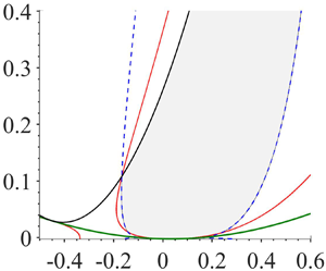
 $D_{\perp } > 0$. In the figure 17 we show the phase stability diagrams for a Newtonian fluid and two different values of the viscosities ratio
 $r$. Curves (1) and (2) correspond to
 $D_{\perp } = 0$ and
 $D_{\parallel } = 0$, respectively. Curve (4) is the upper stability amplitude where a bifurcation to rolls occurs. The minimum of curve (4) is located in the region
 $q < 0$. Below curve (3), no hexagons exist. Hexagons are stable in the shaded region. For viscosities ratio
 $1 \leq r \leq 2$, the region of stability to amplitude and phase modes is closed. Whereas for larger values of
 $r$, the stability domain is open. Note also that the domain of stability is decentred towards the right. It is delimited mainly by the stability amplitude curves and the transverse phase instability boundary. Nevertheless, the numerical results show that close to the threshold, the longitudinal mode is the relevant destabilizing mode. The region where the longitudinal mode destabilizes the pattern increases slightly with increasing
 $r$. Qualitatively, a similar description of the phase stability diagram can be done for a Carreau fluid with low or moderate values of
 $r$ as it is shown in figure 18. Once again, the region where the longitudinal mode is the relevant destabilizing mode remains small and close to the onset. A summary of the results relating to the influence of
 $r$ and
 $\alpha$ on the stability domain of hexagons is given by figure 19(a). With increasing shear-thinning effects, the stability domain becomes more decentred towards the right. Concerning the influence of
 $r$, as discussed before, the thermodependency of the fluid viscosity increases significantly the stability domain of hexagons. For comparison, we have represented in figure 19(b) the stability domain of hexagons when
 $\alpha _1 = \alpha _2 = 0$. This domain is symmetrical with respect to the vertical axis.
Hexagon stability diagram for a Newtonian fluid at  $Pr = 50$ and two different values of the viscosities ratio: (a)
 $r = 1.5$ and (b)
 $r = 2.5$. Hexagons are stable inside the grey area. Curve (1):
 $D_{\perp } = 0$, curve (2)
 $D_{\parallel }=0$, curve (3) bifurcation from the conductive state to convection with hexagons, curve (4) bifurcation from hexagons to rolls.

Hexagon stability diagram for a shear-thinning fluid with  $\alpha = 10^{-4}$ at
 $Pr = 50$ and two different values of the viscosities ratio: (a)
 $r = 1.5$ and (b)
 $r = 2.5$. Hexagons are stable inside the grey area.

Influence of shear-thinning effects and viscosities ratio on the hexagons stability diagram at  $Pr = 50$. (a) Spatial non-variational terms in (4.22) are taken into account, (b)
 $\alpha _1 = \alpha _2 = 0$. Curves (1), (4) and (7) correspond to a Newtonian fluid and three different values of
 $r$:
 $2.5, 2.0, 1.5$, respectively. Curves (2), (5) and (8) correspond to a shear-thinning fluid with
 $\alpha = 5 \times 10^{-5}$. Curves (3), (6) and (9) correspond to a shear-thinning fluid with
 $\alpha = 10^{-4}$.

8. Numerical solutions of amplitude equations
8.1. Numerical simulation
For numerical integration of the Ginzburg–Landau equations (4.22), we employed a Fourier pseudospectral method on a square mesh with periodic boundary conditions. Calculations are carried out in spectral space (wavenumber) with the exception of evaluating nonlinear and conjugate terms which are performed in physical space. The square domain  $[-L/2, L/2 ] \times [-L/2 , L/2 ]$ is discretized into
 $N \times N$ uniformly spaced grid points
 $M_{\ell , p}$ with
 $x_{\ell } = - L/2 + \ell \Delta x$ (similarly for
 $y_p$),
 $\Delta _x = \Delta _y = L/N$ and
 $N$ even. For the temporal discretization, the time domain
 $[0, t_{max} ]$ is discretized with equal time step of width
 $\Delta t$ as
 $t_m = m \Delta t$,
 $m = 0, 1,2, \ldots$. The exponential time differencing method of second order (ETD2) proposed by Cox & Matthews (Reference Cox and Matthews2002) is used. The pseudospectral method is implemented in Matlab. Finally, to check the convergence, several simulations are carried out with an increasing numbers of grid points and refining the time step. For the results presented in this section, the numerical resolution is
 $512 \times 512$ in a square of size
 $L = 5 \times 2 {\rm \pi}/q$ and the time step is fixed at
 $0.01$.
8.2. Numerical results
Numerical simulations were carried out in order to illustrate the nonlinear evolution of the transverse phase instability for a hexagonal pattern in both cases: (i) low values of  $\epsilon$, where practically only hexagons are stable for
 $q >0$; and (ii) larger
 $\epsilon$. We discuss the impact of the non-variational quadratic spatial terms on the competition between rolls and hexagons. Further numerical simulations were done to illustrate the transition rolls-hexagons when
 $\epsilon < \epsilon _r$. In the following, the results are presented for three values of the parameters
 $(\epsilon , q)$, represented by the symbol (
 $+$) in figure 20.
Hexagon stability diagram for a shear-thinning fluid with  $\alpha = 10^{-4}, Pr = 50$ and
 $r =2.5$. The curve
 $\epsilon _r(q)$ is a boundary above which rolls are stable with respect to homogeneous perturbations.
 $(+)$ Points where numerical simulations were performed.

8.2.1. Nonlinear evolution of the transverse instability at low $\epsilon$

The initial condition is a perfect hexagonal pattern with a wavenumber  $k= k_c+0.45$ at
 $\epsilon = 0.1$. The point (
 $\mathcal {P}_1$),
 $\epsilon = 0.1$ and
 $q = 0.45$ in figure 20 is outside the domain where hexagons are stable to phase modes. The other parameters are shear-thinning degree
 $\alpha = 10^{-4}$, viscosity ratio
 $r = 2.5$ and Prandtl number
 $Pr = 50$. At
 $t = 0$, the hexagonal pattern is slightly disturbed.
Figure 21 displays the time evolution of the vertical velocity  $w = \sum _{i=1}^3 A_i(x,y,t) \exp ({\textrm {i} \boldsymbol {k}_{c,i} \boldsymbol {\cdot } \boldsymbol {r}}) + \textrm {c.c.}$. It shows how the transverse phase instability leads to a stable hexagonal pattern after passing through intermediate stages. The breakdown of the initial pattern takes place through the creation of penta-hepta defects (two hexagons are replaced by a pentagon and a heptagon). At
 $t = 10$ most of the penta-hepta defects (PHD) are aggregated along lines perpendicular to wavevectors. Their number decreases with time. At
 $t = 1000$, the number of PHD is quite limited and they are circled in figure 21(c). A zoom is given in figure 22(a). The PHD move and eventually annihilate or disappear at the boundaries. Figure 22 is a focus on one penta-hepta defect. It is shown, figure 22(b–d), that in this process the amplitude of two of the three rolls making up the hexagonal pattern are zero. The phases of the sets of rolls obtained from
 $\arctan ({\rm Im} [A_i(x,y)]/ {\rm Re} [A_i(x,y) ] )$ are represented in figure 23. The phases of two sets of rolls that vanish at the defect present a singularity, while the third one does not have any singularity. Actually, the penta-hepta defect is pictured as a dislocation in each of the sets of rolls whose amplitude vanish at the core of the defect (Ciliberto et al. Reference Ciliberto, Coullet, Lega, Pampaloni and Perez-Garcia1990; Sushchik & Tsimring Reference Sushchik and Tsimring1994; Hoyle Reference Hoyle1995).
Initial condition ( $\mathcal {P}_1$): hexagons with
 $q = 0.45, \epsilon = 0.1, r = 2.5$,
 $\alpha = 10^{-4}$ and
 $Pr = 50$. Contours of the vertical velocity
 $w = \sum _{i=1}^3 A_i \exp ({\textrm {i} \boldsymbol {k}_{c,i} \boldsymbol {\cdot } \boldsymbol {x}}) + \textrm {c.c.}$ for a hexagonal pattern undergoing the transverse instability. The contours are shown at times (a)
 $t = 0$; (b)
 $t = 10$; (c)
 $t = 1000$ and (d)
 $t = 2000$. In panel (c) the penta-hepta defects are circled.

Initial condition ( $\mathcal {P}_1$): hexagons with
 $q = 0.45, \epsilon = 0.1, r = 2.5, \alpha = 10^{-4}$ and
 $Pr = 50$. Focus on one penta-hepta defect at
 $q = 0.45$,
 $r = 2.5$ and
 $\alpha = 10^{-4}$: (a) contours of the ‘vertical velocity’
 $w$ at
 $t = 1000$ with one penta-hepta defect circled. (b) Modulus of
 $A_1$ which vanishes at the core of the defect. (c) Modulus of
 $A_2$, non-zero in the circle (
 $|A_2 = 0.114|$). (d) Modulus of
 $A_3$ which vanishes at the core of the defect.

Initial condition ( $\mathcal {P}_1$): hexagons with
 $q = 0.45, \epsilon = 0.1, r = 2.5, \alpha = 10^{-4}$ and
 $Pr = 50$. (a) Contours of the vertical velocity
 $w = \sum _{i=1}^3 A_i \exp ({\textrm {i} \boldsymbol {k}_{c,i} \boldsymbol {\cdot } \boldsymbol {x}}) + \textrm {c.c.}$ at
 $t = 1000$; (b) phase of
 $A_1$; (c) phase of
 $A_2$ and (d) phase of
 $A_3$.

8.2.2. Nonlinear evolution of the transverse phase instability at large $\epsilon$

In the previous section we considered a rather small  $\epsilon$ for which hexagons are the only possible state. A completely different final state of the transverse phase instability is observed for larger
 $\epsilon$, i.e.
 $\epsilon$ greater than a threshold value
 $\epsilon ^*$. Figure 24 shows the nonlinear evolution of the convection pattern when the initial condition, point
 $\mathcal {P}_2$ in figure 20, consists of a perfect hexagon at
 $\epsilon =0.3$, with a wavenumber,
 $k=k_c+0.55$, outside the phase stability domain. The other parameters are
 $\alpha = 10^{-4}, r = 2.5$ and
 $Pr = 50$. In this case, the transverse phase instability triggers the transition from a regular hexagonal pattern to a disordered roll state with several grain boundaries. The threshold value
 $\epsilon ^*$ at which the transition to rolls occurs can only be determined by numerical simulations due to the lack of Lyapunov functional for (4.22). For the particular case considered here,
 $q = 0.55, r = 2.5, \alpha = 10^{-4}$ and
 $Pr = 50$, we have found
 $\epsilon ^* \approx 0.22$.
Initial condition ( $\mathcal {P}_2$): hexagons with
 $q = 0.55, \epsilon = 0.3, r = 2.5$,
 $\alpha = 10^{-4}$ and
 $Pr = 50$. The reconstructed vertical velocity
 $w$ is shown at different times: (a)
 $t = 0$, (b)
 $t = 2$, (c)
 $t = 10$ and (d)
 $t = 100$.

Although at  $\epsilon = 0.3$ hexagons are linearly stable to homogeneous perturbations as shown in figure 14(b), when defects first appear, the dynamics may change. According to Sushchik & Tsimring (Reference Sushchik and Tsimring1994) and Ciliberto et al. (Reference Ciliberto, Coullet, Lega, Pampaloni and Perez-Garcia1990), the presence of defects in a system plays an important role in the dynamics of transition between rolls and hexagons. In our case, pieces of rolls appear in the beginning. Under certain conditions, they spread and destroy the hexagonal pattern. Furthermore, it is observed that the time necessary to reach the steady state is much lower for large
 $\epsilon$.
8.2.3. Rolls–hexagons transition
Figure 25 shows the contours of the reconstructed vertical velocity  $w$ at different times in the case where the initial data, point
 $\mathcal {P}_3$ in figure 20, correspond to perfect rolls at
 $\epsilon = 0.1$,
 $q = 0.25$ for a Carreau fluid with
 $\alpha = 10^{-4}$ and
 $Pr = 50$. According to figure 14(b), these rolls are unstable. This is confirmed by the computation, in which the final state consists of hexagons. We note that the transition from rolls to hexagons undergoes pearling, which gradually leads to separation into hexagons similarly as in Van-Den-Berg et al. (Reference Van-Den-Berg, Deschênes, Lessard and Mireles-James2015).
Remark When there is no distortion of hexagons, i.e. when  $\alpha _1 = \alpha _2 = 0$, in (4.22), the competition between uniform rolls and uniform hexagons is governed by the free energy density difference between them as indicated by Young & Riecke (Reference Young and Riecke2002), Sushchik & Tsimring (Reference Sushchik and Tsimring1994) and Hoyle (Reference Hoyle2006). For a given wavenumber
 $k = k_c + q$, hexagons have lower energy than rolls, and, therefore, are more stable at
 $\epsilon$ lower than a threshold value
 $\epsilon _f$ at which rolls and hexagons have the same free energy. Rolls are energetically favoured above
 $\epsilon _f$. To determine
 $\epsilon _f$, we compare the free energy density for perfect rolls,
 \begin{equation} F_r = - \frac{\epsilon - q^2 \xi_0^2}{\tau_0} R_0^2 + \frac{g_1}{2} R_0^4 , \end{equation}
Initial condition ( $\mathcal {P}_3$): rolls with
 $q = 0.25, \epsilon = 0.1, r = 2.5$,
 $\alpha = 10^{-4}$ and
 $Pr = 50$. The reconstructed vertical velocity
 $w$ is shown at different times: (a)
 $t = 0$, (b)
 $t = 11$, (c)
 $t = 15$ and (d)
 $t = 2000$.

and for perfect hexagons,
 \begin{equation} F_h = - 3 \frac{\epsilon - q^2 \xi_0^2}{\tau_0} H_0^2 -2 \zeta H_0^3 + \frac{3}{2} \left( g_1 + 2 g_2\right) H_0^4 . \end{equation}
It can be shown that  $F_r = F_h$ at
 \begin{equation} \epsilon_f = \frac{\tau_0 \zeta^2 \left[g_1^2 + 3 g_1 g_2 + \sqrt{2 g_1} \left(g_1 + g_2 \right)^{3/2}\right]}{2 \left(g_2 + 2 g_2 \right) \left(g_1 - g_2 \right)^2} + q^2 \xi_0^2 . \end{equation}
Figure 26 shows the variation of  $\epsilon _f$ with the shear-thinning degree
 $\alpha$ for
 $q = 0.55, r = 2.5$ and
 $Pr = 50$. The nonlinearity of the rheological law favours rolls rather than hexagons. Values of
 $\epsilon _f$ are found higher (but in reasonable agreement) than the real threshold for hexagon–roll transition obtained from our numerical simulations. As explained by Sushchik & Tsimring (Reference Sushchik and Tsimring1994), the difference is due to the fact that the simple energetic analysis used in the determination of
 $\epsilon _f$ does not take into account the non-uniform structure of defects. Note that when
 $\alpha _1 = \alpha _2 = 0$, the final state consists of perfect rolls or perfect hexagons.
Threshold for hexagon–roll transition in the case where there is no distortion of hexagons as a function of the shear-thinning degree, with  $q=0.55, r = 2.5$ and
 $Pr = 50$. (1) Curve of equal energy for hexagons and rolls, (2) numerical simulations.

9. Conclusion
We have investigated the influence of shear-thinning effects on Rayleigh–Bénard convection for a Carreau fluid, taking into account the variation of the viscosity with temperature. The dependence of the viscosity on temperature was assumed of exponential type. A weakly nonlinear analysis using a multiple scale is adopted as a first approach to investigate the nonlinear effects. Generalized Ginzburg–Landau equations are obtained including spatial non-variational terms which account for the distortion of hexagons. The coefficients of these equations have been explicitly calculated and correlations are proposed. The steady solutions of these equations that correspond to rolls and hexagons have been obtained and their relative stability has been determined. Past the onset of convection, hexagonal cells with upward motion in the centre are selected in agreement with the experimental results of Darbouli et al. (Reference Darbouli, Métivier, Leclerc, Nouar and Stemmlen2016) and Bouteraa (Reference Bouteraa2016). The range of Rayleigh numbers associated with the subcritical convection is very narrow ( $|\epsilon _h| \ll 1$) and difficult to detect experimentally. It is all the more reduced as shear-thinning effects are strong. For higher supercritical values, coexistence between hexagons and rolls is predicted in agreement with the experimental observations of Darbouli et al. (Reference Darbouli, Métivier, Leclerc, Nouar and Stemmlen2016) and Bouteraa (Reference Bouteraa2016). The range of
 $Ra$ for which hexagons are stable increases with increasing viscosity ratio and decreases with increasing shear-thinning effects. This behaviour is along the same lines as the conclusion of Bouteraa et al. (Reference Bouteraa, Nouar, Plaut, Métivier and Kalck2015), where it is shown that the nonlinearities introduced by the rheological law reinforce the stability of rolls. The stability of hexagons with respect to long wavelength perturbations is then addressed. Phase equations are derived and the band of stable wavenumbers is determined. Two types of long wavelength instabilities are identified: longitudinal and transverse phase instabilities. It is found that the stable hexagons domain is delimited mainly by the transverse phase instability. Furthermore, it is shown that the additional spatial nonlinear terms break the symmetry around
 $k_c$: the band of stable wavenumbers is open and decentred to the right, i.e. to wavenumbers larger than the critical one. This result is likewise in agreement with the experimental observations of M. Bouteraa (personal communication 2020), where the measured wavenumber increases with
 $Ra$. The theoretical calculations predict also that the band of stable wavenumbers becomes more decentred with increasing shear-thinning effects.
The numerical integration of the amplitude equations supports the theoretical results, enables us to illustrate the nonlinear evolution of the transverse phase instability and highlights the role of the non-variational terms in the dynamics of pattern formation. At low  $\epsilon$, the transition from perfect hexagons, with a wavenumber outside the stable domain, to a new hexagonal pattern involves penta-hepta defects. Their number, large in the beginning of the process, decreases with time. For larger
 $\epsilon > \epsilon ^*$, the transverse phase instability triggers the transition from regular hexagons to a disordered state of rolls with grain boundaries. The impact of the non-variational terms in the amplitude equations on the pattern dynamics is discussed. We have also performed a numerical simulation starting from a given initial pattern of rolls at
 $\epsilon < \epsilon _r$. The rolls-hexagons transition occurs through a progressive pearling leading to the creation of spots.
This study will be continued by considering larger values of the viscosity ratio  $r$, for which we have a competition between squares and hexagons. In addition it would be useful to consider the temperature-dependence of other material properties such as the volumetric thermal expansion coefficient. There are other possible areas of future work. For instance, an investigation could be carried out to include side wall effects. Also, it would be interesting to analyse the influence of defects (pentagon-heptagon pair), which emerge in the hexagonal pattern, on the transition between different symmetries as well as on the wavenumber selection. Finally, we hope that the present work suggests new experiments to study the influence of shear-thinning effects on the selection of the convective pattern and its stability for high supercritical values of
 $Ra$, using experimental apparatus of larger aspect ratio comparatively to Darbouli et al. (Reference Darbouli, Métivier, Leclerc, Nouar and Stemmlen2016) and Bouteraa (Reference Bouteraa2016).
Appendix A. Operators and matrix coefficients
The coefficients of the matrices in (4.7)–(4.8) are given below:
A.1. The operator ${M}$

 \begin{equation} \boldsymbol{M} = \begin{pmatrix} M_{11} & 0 & 0 & 0 \\ M_{21} & M_{22} & 0 & 0 \\ M_{31} & 0 & M_{33} & 0 \\ 0 & 0 & 0 & 1 \end{pmatrix}, \end{equation}
with
 \begin{equation} \left. \begin{gathered} M_{11} = Pr^{-1} \Delta , \quad M_{21} = \frac{\partial^2 }{\partial x \partial z} , \quad M_{22} = \boldsymbol{\nabla}_{Hx}^2 ,\\ M_{31} = \frac{\partial^2 }{\partial y \partial z} , \quad M_{33} = \boldsymbol{\nabla}_{Hx}^2. \end{gathered} \right\} \end{equation}
A.1.1. The sub-scale ${M}^{(0)}$

The coefficients of  $\boldsymbol {M}^{(0)}$ in (4.7) are
 \begin{equation} \left. \begin{gathered} M^{(0)}_{11} = Pr^{-1} \left(\Delta_{Hx} + \frac{\partial^2}{\partial z^2} \right) , \\ M^{(0)}_{21} = \frac{\partial^2}{\partial x \partial z} ,\quad M^{(0)}_{22} = \Delta_{Hx} , \\ M^{(0)}_{31} = \frac{\partial^2}{\partial y \partial z} ,\quad M^{(0)}_{33} = \Delta_{Hx} , \\ M^{(0)}_{44} = 1 . \end{gathered} \right\} \end{equation}
A.1.2. The sub-scale ${M}^{(1)}$

The coefficients of  $\boldsymbol {M}^{(1)}$ in (4.7) are
 \begin{equation} \left. \begin{gathered} M^{(1)}_{11} = 2 \, Pr^{-1} \, \boldsymbol{\nabla}_{Hx} \boldsymbol{\cdot} \boldsymbol{\nabla}_{HX},\\ M^{(1)}_{21} = \frac{\partial^2}{\partial X \partial z} , \quad M^{(1)}_{22} = 2 \quad \boldsymbol{\nabla}_{Hx} \boldsymbol{\cdot} \boldsymbol{\nabla}_{HX} ,\\ M^{(1)}_{31} = \frac{\partial^2}{\partial Y \partial z} , \quad M^{(1)}_{33} = 2 \quad \boldsymbol{\nabla}_{Hx}\boldsymbol{\cdot} \boldsymbol{\nabla}_{HX} ,\\ M^{(1)}_{44}=0. \end{gathered} \right\} \end{equation}
A.2. The operator ${L}$

The coefficients of the  $4 \times 4$ matrix
 $\boldsymbol {L}$ in (2.20) are given by
 \begin{equation} L = \begin{pmatrix} L_{11} & 0 & 0 & L_{14} \\ L_{21} & L_{22} & 0 & 0 \\ L_{31} & 0 & L_{33} & 0 \\ 1 & 0 & 0 & \Delta \end{pmatrix}, \end{equation}
with
 \begin{equation} \left. \begin{gathered} L_{11} = \mu_b \Delta^2 + 2 \frac{\text{d} \mu_b}{\text{d}z} \Delta \frac{\partial}{\partial z} + \frac{\textrm{d}^2 \mu_b}{\textrm{d} z^2} \left(\frac{\partial^2 }{\partial z^2} - \Delta_H \right) , \quad L_{14} = Ra\, \Delta_H ,\\ L_{21} = \mu_b \Delta \frac{\partial ^2}{\partial x \partial z} + \frac{\textrm{d} \mu_b}{\textrm{d} z} \frac{\partial}{\partial z} \left(\frac{\partial^2}{\partial x \partial z}\right) , \quad L_{22} = \mu_b \Delta \Delta_H + \frac{\textrm{d} \mu_b}{\textrm{d} z} \frac{\partial}{\partial z} \Delta_H ,\\ L_{31} = \mu_b \Delta \frac{\partial ^2}{\partial y \partial z} + \frac{\textrm{d} \mu_b}{\textrm{d} z} \frac{\partial}{\partial z} \left(\frac{\partial^2}{\partial y \partial z}\right) , \quad L_{33} = \mu_b \Delta \Delta_H + \frac{\textrm{d} \mu_b}{\textrm{d} z} \frac{\partial}{\partial z} \Delta_H . \end{gathered} \right\} \end{equation}
A.3. Sub-scale ${L}^{(0)}$

The components of  $\boldsymbol {L}^{(0)}$ in (4.8) are
 \begin{equation} \left. \begin{gathered} L^{(0)}_{11} = \mu_b \left(\boldsymbol{\nabla}_{Hx}^2 + \frac{\partial^2}{\partial z^2}\right)^2 + 2 \frac{\textrm{d} \mu_b}{\textrm{d} z} \left(\boldsymbol{\nabla}_{Hx}^2 + \frac{\partial^2}{\partial z^2} \right) \frac{\partial}{\partial z} + \frac{\textrm{d}^2 \mu_b}{\textrm{d} z^2} \left( \frac{\partial^2}{\partial z^2} - {\nabla}^2_{Hx} \right) , \\ L_{14}^{(0)} = Ra_c \boldsymbol{\nabla}_{Hx}^2 ,\\ L_{21}^{(0)} = \mu_b \left(\boldsymbol{\nabla}_{Hx}^2 + \frac{\partial^2}{\partial z^2}\right) \frac{\partial ^2}{\partial x \partial z} + \frac{\textrm{d} \mu_b}{\textrm{d} z} \frac{\partial}{\partial z} \left(\frac{\partial^2}{\partial x \partial z}\right) , \\ L_{22}^{(0)} = \mu_b \left(\boldsymbol{\nabla}_{Hx}^2 + \frac{\partial^2}{\partial z^2}\right) \boldsymbol{\nabla}_{Hx}^2 + \frac{\textrm{d} \mu_b}{\textrm{d} z} \frac{\partial}{\partial z} \boldsymbol{\nabla}_{Hx}^2,\\ L_{31}^{(0)} = \mu_b \left(\boldsymbol{\nabla}_{Hx}^2 + \frac{\partial^2}{\partial z^2}\right) \frac{\partial ^2}{\partial y \partial z} + \frac{\textrm{d} \mu_b}{\textrm{d} z} \frac{\partial}{\partial z} \left(\frac{\partial^2}{\partial y \partial z}\right) , \\ L_{33}^{(0)} = L_{22}^{(0)} ,\\ L_{41}^{(0)} = 1 , \quad L_{44}^{(0)} = \left(\boldsymbol{\nabla}_{Hx}^2 + \frac{\partial^2}{\partial z^2} \right) . \end{gathered} \right\} \end{equation}
A.4. Sub-scale ${L}^{(1)}$

The components of  $\boldsymbol {L}^{(1)}$ in (4.8) are
 \begin{equation} \left. \begin{gathered} L_{11}^{(1)} \!=\! 4 \mu_b \left(\boldsymbol{\nabla}_{Hx}^2 \!+\! \frac{\partial^2}{\partial z^2} \right) \left( \boldsymbol{\nabla}_{Hx} \boldsymbol{\cdot} \boldsymbol{\nabla}_{HX}\right) + 4 \, \frac{\textrm{d} \mu_b}{\textrm{d} z} \left(\boldsymbol{\nabla}_{Hx} \boldsymbol{\cdot} \boldsymbol{\nabla}_{HX} \right)\frac{\partial}{\partial z} - 2 \frac{\textrm{d}^2 \mu_b}{\textrm{d} z^2} \left(\boldsymbol{\nabla}_{Hx} \boldsymbol{\cdot} \boldsymbol{\nabla}_{HX} \right),\\ L_{14}^{(1)} = Ra^{(1)} \boldsymbol{\nabla}_{Hx}^2 + 2 Ra_c \left(\boldsymbol{\nabla}_{Hx} \boldsymbol{\cdot} \boldsymbol{\nabla}_{HX} \right) ,\\ L_{21}^{(1)} = \mu_b \left(\boldsymbol{\nabla}_{Hx}^2 + \frac{\partial^2}{\partial z^2} \right) \frac{\partial^2}{\partial X \partial z} + 2 \mu_b \left(\boldsymbol{\nabla}_{Hx} \boldsymbol{\cdot} \boldsymbol{\nabla}_{HX} \right) \frac{\partial^2}{\partial x \partial z} + \frac{\text{d} \mu_b}{\text{d} z} \frac{\partial^2}{\partial z^2} \frac{\partial }{\partial X},\\ L_{22}^{(1)} = 2 \mu_b \left[\frac{\partial^2}{\partial z^2} + 2 \left(\frac{\partial^2}{\partial x^2} + \frac{\partial^2}{\partial y^2} \right)\right] \left(\boldsymbol{\nabla}_{Hx} \boldsymbol{\cdot} \boldsymbol{\nabla}_{HX}\right) + 2 \frac{\textrm{d} \mu_b}{\textrm{d} z} \left(\boldsymbol{\nabla}_{Hx} \boldsymbol{\cdot} \boldsymbol{\nabla}_{HX} \right) \frac{\partial}{\partial z},\\ L_{31}^{(1)} = \mu_b \left[{\boldsymbol{\nabla}}_{Hx}^2 \frac{\partial^2}{\partial Y \partial z} + 2 \, \boldsymbol{\nabla}_{Hx} \boldsymbol{\cdot} \boldsymbol{\nabla}_{HX} + \frac{\partial^2}{\partial z^2} \frac{\partial^2}{\partial Y \partial z}\right] + \frac{\textrm{d} \mu_b}{\textrm{d} z} \frac{\partial^2}{\partial z^2} \frac{\partial }{\partial Y},\\ L_{41}^{(1)} = 0 , \quad L_{44}^{(1)} = 2 \boldsymbol{\nabla}_{Hx} \boldsymbol{\cdot} \boldsymbol{\nabla}_{HX} . \end{gathered} \right\} \end{equation}
A.5. Sub-scale ${L}^{(2)}$

The components of  $\boldsymbol {L}^{(2)}$ in (4.8) are
 \begin{equation} \left. \begin{gathered} L_{11}^{(2)} = \mu_b \left[2 \left(\boldsymbol{\nabla}_{Hx}^2 + \frac{\partial^2}{\partial z^2} \right) \boldsymbol{\nabla}_{HX}^2 + 4 \left(\boldsymbol{\nabla}_{Hx} \boldsymbol{\cdot} \boldsymbol{\nabla}_{HX} \right)^2\right] + 2\, \frac{\textrm{d} \mu_b}{\textrm{d} z} \boldsymbol{\nabla}_{HX}^2 \, \frac{\partial}{\partial z} - \frac{\textrm{d}^2 \mu_b}{\textrm{d} z^2} \boldsymbol{\nabla}_{HX}^2,\\ L_{14}^{(2)} = Ra_c {\boldsymbol{\nabla}}_{HX}^2 + 2 Ra^{(1)} \left({\boldsymbol{\nabla}}_{Hx} \boldsymbol{\cdot} {\boldsymbol{\nabla}}_{HX} \right) + Ra^{(2)} {\boldsymbol{\nabla}}_{Hx}^2 ,\\ L_{21}^{(2)} = \mu_b\, \left[ 2 \left(\boldsymbol{\nabla}_{Hx} \boldsymbol{\cdot} \boldsymbol{\nabla}_{HX} \right) \frac{\partial^2}{\partial X \partial z} + \boldsymbol{\nabla}_{HX}^2 \frac{\partial^2}{\partial x \partial z}\right],\\ L_{22}^{(2)} = \mu_b \left(\frac{\partial^2}{\partial z^2} + \boldsymbol{\nabla}_{Hx}^2\right) \boldsymbol{\nabla}_{HX}^2 + 4 \mu_b \left(\boldsymbol{\nabla}_{Hx} \boldsymbol{\cdot} \boldsymbol{\nabla}_{HX} \right)^2 + \mu_b \boldsymbol{\nabla}_{HX}^2 \boldsymbol{\nabla}_{Hx}^2,\\ L_{31}^{(2)} = \mu_b\, \left[ 2 \left(\boldsymbol{\nabla}_{Hx} \boldsymbol{\cdot} \boldsymbol{\nabla}_{HX} \right) \frac{\partial^2}{\partial Y \partial z} + \boldsymbol{\nabla}_{HX}^2 \frac{\partial^2}{\partial y \partial z}\right],\\ L_{41}^{(2)} = 0 , \quad L_{44}^{(2)} = \boldsymbol{\nabla}_{HX}^2. \end{gathered} \right\} \end{equation}
Appendix B. Second-order solution (hexagons)
B.1. Solution proportional to $|A_p|^2$ (zero mode)

The first component of the second-order solution, proportional to  $|A_p|^2$, provides a correction of the basic state. Considering the
 $w$-equation, it is shown that the factor of
 $|A_1|^2, |A_2|^2$ and
 $|A_3|^2$ in the nonlinear inertial
 $NI_w^{(2)}$ and viscous
 $NV^{(2)}_w$ terms vanishes; therefore,
 \begin{equation} w^{(2)}_{1} = 0 . \end{equation}
Here  $w_1^{(2)}$ means the first component of the second-order solution. Similarly, for the horizontal velocity, we have
 \begin{equation} u^{(2)}_{1} = v^{(2)}_{1} = 0 . \end{equation}
There is no velocity for the zero mode. The correction of the conductive temperature profile can be written as  $\theta ^{(2)}_1 = T_1(z) [|A_1|^2 + |A_2|^2 + |A_3|^2]$, where
 $T_1(z)$ satisfies
 \begin{equation} D^2 T_{1} = 2 \left [G_{11} \left(DF_{11}\right) + F_{11} \left(DG_{11}\right) \right) , \end{equation}
with
 \begin{equation} T_{1} = 0 \quad \text{at} \ z = 0 \ \text{and} \ z = 1. \end{equation}
As for the linear problem, (B 3) with the boundary conditions (B 4) is solved numerically using a spectral Chebyshev collocation method.
B.2. Solution proportional to $A_{p}^{2}$ exp (2i $k_{\textit{p}}\,{\cdot}\,r)$


The second component of the second-order solution, proportional to  $A_p^2 E_p^2$, where
 $E_p=\exp (\textrm {i}\boldsymbol {k}_{p}\boldsymbol {\cdot }\boldsymbol {r})$ represents the first harmonic of the fundamental. We have
 \begin{equation} \left(w_2^{(2)}, \theta_2^{(2)} \right) = \left(W_2(z), T_2(z) \right)) \left(A_1^2 E_1^2 + A_2^2 E_2^2 + A_3^2 E_3^2 \right) + \textrm{c.c.}, \end{equation}
with
 \begin{align} &\left[\mu_b \left(D^2 - 4 k_c^2 \right)^2 + 2 \frac{\textrm{d} \mu_b}{\textrm{d} z} \left(D^3 - 4 k_c^2 D \right) + \frac{\textrm{d}^2 \mu_b}{\textrm{d} z ^2} \left(D^2 + 4 k_c^2 \right)\right] W_{2} - 4 k_c^2 Ra_c T_{2}\nonumber\\ &\quad = \frac{2}{Pr} \left(F_{11} D^3 F_{11} - DF_{11} D^2F_{11} \right) - \left[NV_w\right]^{(2)}_{A_p^2 E_p^2} , \end{align}
 \begin{equation} W_2 + \left(D^2 - 4 k_c^2 \right)T_2 = F_{11} DG_{11} - G_{11} DF_{11} . \end{equation}
The boundary conditions on  $W_{2}$ and
 $T_{2}$ are identical to those on
 $F_{11}$ and
 $G_{11}$, (3.4).
Concerning the horizontal velocity, we have
 \begin{equation} \boldsymbol{\nabla}_{Hx}^2 \boldsymbol{u}_{H2}^{(2)} + \boldsymbol{\nabla}_{Hx} \frac{\partial w^{(2)}_2}{\partial z} = 0 . \end{equation}
We obtain
 \begin{equation} \boldsymbol{u}^{(2)}_{H2} = \frac{D W_2}{4 k_c^2} \boldsymbol{\nabla}_{Hx} \left[A_1^2 E_1^2 + A_2^2 E_2^2 + A_3^2 E_3^2 \right] + \textrm{c.c.} \end{equation}
B.3. Solution proportional to $A_p A_q^* E_p E_q^*$

The third component of the second-order solution, proportional to  $A_p A_q^* E_p E_q^*$, reads as
 \begin{equation} \left(w^{(2)}_3 , \theta^{(2)}_3 \right) = \left(W_3(z), T_3(z) \right) \left(A_1 A_2^* E_1 E_2^* + A_1 A_3^* E_1 E_3^* + A_2 A_3^* E_2 E_3^*\right) + \textrm{c.c.}, \end{equation}
with
 \begin{align} &\left[\mu_b \left(D^2 - 3 k_c^2 \right)^2 + 2 \frac{\textrm{d} \mu_b}{\textrm{d} z} \left(D^3 - 3 k_c^2 D \right) + \frac{\textrm{d}^2 \mu_b}{\textrm{d} z ^2} \left(D^2 + 3 k_c^2 \right)\right] W_3 - 3 k_c^2 Ra_c T_3\nonumber\\ &\quad = \frac{3}{Pr} \left(F_{11}D^3 F_{11} - k_c^2 F_{11} DF_{11} \right) - \left[NV_w \right]_{E_p E_{q^*}}^{(2)}, \end{align}
 \begin{equation} W_3 + \left(D^2 - 3 k_c^2 \right) T_3 = 2 F_{11} DG_{11} - G_{11} DF_{11}. \end{equation}
Boundary conditions on  $(W_3, T_3)$ are the same as the ones on
 $(F_{11}, G_{11} )$.
The horizontal velocity components satisfy
 \begin{equation} \boldsymbol{\nabla}_{Hx}^2 \boldsymbol{u}^{(2)}_{H3} + \boldsymbol{\nabla}_{Hx} \frac{\partial w^{(2)}_3}{\partial z} = 0. \end{equation}
We obtain
 \begin{equation} \boldsymbol{u}^{(2)}_{H3} = \frac{D W_3}{3 k_c^2} \boldsymbol{\nabla}_{Hx} \left(A_1 A_2^* E_1 E_2^* + A_1 A_3^* E_1 E_3^* + A_2 A_3^* E_2 E_3^*\right) + \textrm{c.c.} \end{equation}
B.4. Solution proportional to exp (i ${k}_{\textit{p}} \, {\cdot } \, {r})$

The fourth component of the second-order solution is proportional to  $\exp (\textrm {i} \boldsymbol {k}_{p} \boldsymbol {\cdot } \boldsymbol {r} )$ (resonant term). The solution is achieved using the solvability condition. It is shown that it can be written as
 \begin{equation} \left(w^{(2)}_4 , \theta^{(2)}_4\right) = \left(W_{41}, T_{41}\right) E_1 + \left(W_{42}, T_{42} \right) E_2 + \left(W_{43}, T_{43} \right) E_3 + \textrm{c.c.}, \end{equation}
with
 \begin{align} &\left[\mu_b \left(\frac{\partial^2}{\partial z^2} - k_c^2 \right)^2 + 2 \frac{\textrm{d} \mu_b}{\textrm{d} z} \left(\frac{\partial^2}{\partial z^2} - k_c^2 \right) \frac{\partial}{\partial z} + \frac{\textrm{d}^2 \mu_b}{\textrm{d} z ^2} \left(\frac{\partial^2}{\partial z^2} + k_c^2 \right)\right] W_{41} - Ra_c k_c^2 T_{41} \nonumber\\ &\quad = \left[- 4 \textrm{i} \mu_b \left(D^2 - k_c^2 \right) F_{11} - 4 \textrm{i} \frac{\textrm{d} \mu_b}{\textrm{d} z} DF_{11} + 2 \textrm{i} \frac{\textrm{d}^2 \mu_b}{\textrm{d} z^2} F_{11}\right] \left(\boldsymbol{k}_1 \boldsymbol{\cdot} \boldsymbol{\nabla}_{HX} \right) A_1 \nonumber\\ &\qquad + k_c^2 \, Ra_1 \, G_{11} A_1 - 2 \textrm{i} Ra_c G_{11} \left(\boldsymbol{k}_2 \boldsymbol{\cdot} \boldsymbol{\nabla}_{HX} \right) A_1\nonumber\\ &\qquad + \frac{1}{Pr} \left(F_{11}D^3 F_{11} + 2 DF_{11} D^2 F_{11} - 3 k_c^2 F_{11} DF_{11}\right) A_2^* A_3^* - \left[NV_w^{(2)}\right]_{E_1} A_2^* A_3^*, \end{align}
 \begin{equation} W_{41} + \left(D^2 - k_c^2 \right) T_{41} = - 2 \textrm{i} G_{11} \left(\boldsymbol{k}_1 \boldsymbol{\cdot} \boldsymbol{\nabla}_{HX} \right) A_1 + \left(2 F_{11} D G_{11} + G_{11} DF_{11} \right) A_2^* A_3^* . \end{equation}
Two others similar systems of equations are obtained for  $(W_{42}, T_{42} )$ and
 $(W_{43}, T_{43} )$ by the circular permutation of indices. Note that according to (4.18),
 ${Ra}^{(1)} A_1$ can be written in terms of
 $A_2^* A_3^*$. The system of differential equations (B 16), (B 17) can be written formally as
 $[\boldsymbol {A}] (W_{41}, T_{41} )^t = [\boldsymbol {X}]A_2^* A_3^* + \boldsymbol {Z} (2 \textrm {i}) (\boldsymbol {k}_1 \boldsymbol {\cdot } \boldsymbol {\nabla }_{HX}) A_1$.
Hence,  $(W_{41}, T_{41} )^t=(W_s, T_s )^t A_2^* A_3^* + (\tilde {W}_s, \tilde {T}_s )^t 2 \textrm {i} (\boldsymbol {k_1} \boldsymbol {\cdot } \boldsymbol {\nabla }_{HX} ) A_1$, where
 $(W_s, T_s )^t = [\boldsymbol {A} ]^{-1} [\boldsymbol {X} ]$ and
 $(\tilde {W}_s, \tilde {T}_s )^t = [\boldsymbol {A} ]^{-1} [\boldsymbol {Z} ]$. The boundary conditions on
 $W_{s}$ and
 $T_{s}$ are the same as the ones on
 $(F_{11}, G_{11})$.
For the horizontal velocity, we have
 \begin{equation} \boldsymbol{u}^{(2)}_{H4} = \boldsymbol{U}_{H41} E_1 + \boldsymbol{U}_{H42} E_2 + \boldsymbol{U}_{H43} E_3 + \textrm{c.c.}, \end{equation}
with
 \begin{align} &\mu_b \left(\frac{\partial^2}{\partial z^2} - k_c^2 \right) \left(-k_c^2 \boldsymbol{U}_{H41} + \textrm{i} \boldsymbol{k}_1 \frac{\partial W_{41}}{\partial z} \right)\nonumber\\ &\quad + \frac{\textrm{d} \mu_b}{\textrm{d} z} \left(-k_c^2 \frac{\partial}{\partial z} \boldsymbol{U}_{H41} + \textrm{i} \boldsymbol{k}_1 \frac{\partial^2 W_{41}}{\partial z^2} \right) = 2 \frac{\textrm{d} \mu_b}{\textrm{d} z} D^2 F_{11} \boldsymbol{\nabla}_{HX} A_1\nonumber\\ &\quad + \left[\mu_b \left(D^3 F_{11} - k_c^2 DF_{11} \right) + \frac{\textrm{d} \mu_b}{\textrm{d} z} D^2 F_{11} \right] \left[2 \frac{\boldsymbol{k}_1}{k_c^2} \left(\boldsymbol{k}_1 \boldsymbol{\cdot} \boldsymbol{\nabla}_{HX}\right) A_1 - \boldsymbol{\nabla}_{HX} A_1 \right]. \end{align}
Two other similar equations are obtained for  $\boldsymbol {U}_{H42}$ and
 $\boldsymbol {U}_{H43}$.
Appendix C. Adjoint eigenvalue problem: adjoint mode
In the analysis developed in § 4, it is necessary to eliminate secular terms in non-homogeneous differential equations, i.e. the solvability condition must be applied. It is therefore necessary to determine the linear adjoint of the direct problem at the critical conditions. For vector fields  $\boldsymbol {f}$ and
 $\boldsymbol {g}$, one defines an inner product between two vector functions
 $\boldsymbol {f}(z)$ and
 $\boldsymbol {g}(z)$ by
 \begin{equation} \left\langle \,\boldsymbol{f} , \boldsymbol{g}\right\rangle = \int_0^1 \boldsymbol{f}^* \boldsymbol{\cdot} \boldsymbol{g}\, \text{d}z , \end{equation}
where  $\boldsymbol {f}^*$ is the complex conjugate of
 $\boldsymbol {f}$. To the direct eigenvalue problem (3.5) corresponds the adjoint problem
 \begin{equation} s \tilde{\boldsymbol{{M}}}^+ \boldsymbol{\cdot} \boldsymbol{{X}_{ad}} = \tilde{\boldsymbol{{L}}}^+ \boldsymbol{\cdot} \boldsymbol{{X}_{ad}} \quad \text{with} \ \boldsymbol{X}_{ad}=(F_{ad}, G_{ad}), \end{equation}
where the adjoint operators  $\tilde {\boldsymbol {M}}^+$ and
 $\tilde {\boldsymbol {L}}^+$ are defined by
 \begin{equation} \langle \boldsymbol{X}_{ad}, \tilde{\boldsymbol{M}} \boldsymbol{\cdot} \boldsymbol{X}_{11}\rangle = \langle \tilde{\boldsymbol{M}}^+ \boldsymbol{\cdot} \boldsymbol{X}_{ad}, \boldsymbol{X}_{11} \rangle , \quad \langle \boldsymbol{X}_{ad}, \tilde{\boldsymbol{L}} \boldsymbol{\cdot} \boldsymbol{X}_{11} \rangle = \langle \tilde{\boldsymbol{L}}^+ \boldsymbol{\cdot} \boldsymbol{X}_{ad}, \boldsymbol{X}_{11} \rangle, \end{equation}
where  $\boldsymbol {X}_{11}$ fulfils the ‘linear’ boundary conditions (3.4). By integrating by parts we get the linear adjoint problem and the corresponding boundary conditions
 \begin{align} &s {Pr}^{-1} \left(D^2 - k^2 \right) F_{ad} = \mu_b \left(D^2 - k^2\right)^2 F_{ad} + 2 D \mu_b \left(D^2 - k^2\right)) D F_{ad} \nonumber\\ & \quad + D^2 \mu_b \left(D^2 + k^2 \right) F_{ad} + G_{ad}, \end{align}
 \begin{equation} s G_{ad} = - k^2\, Ra \, F_{ad} + \left(D^2 - k^2\right) G_{ad}, \end{equation}
with
 \begin{gather} F_{ad} = 0 , \quad D F_{ad} = 0, \quad G_{ad} = 0 \quad \text{at} \ z = 0, \end{gather}
 \begin{gather} F_{ad} = 0 , \quad D F_{ad} = 0, \quad G_{ad} = 0 \quad \text{at} \ z = 1. \end{gather}
The solution of these equations is obtained using the same method as for the direct eigenvalue problem. Similarly, the normalization adopted for the adjoint mode is
 \begin{equation} G_{ad}\left(z = 1/2\right) = 1. \end{equation}
At  $Ra = Ra_c$, the so-called adjoint critical mode does not depend on the Prandtl number.
Appendix D. Cubic-order solution
At order  $\delta ^3$, we have
 \begin{align} &L_{11}^{(0)} w^{(3)} + L_{14}^{(0)} \theta^{(3)}= M_{11}^{(0)} \frac{\partial}{\partial T} w^{(1)} - L_{11}^{(1)} w^{(2)} - L_{14}^{(1)} \theta^{(2)} \nonumber\\ &\quad - L_{11}^{(2)} w^{(1)} - L_{14}^{(2)} \theta^{(1)} - NI_w^{(3)} - NV_w^{(3)} , \end{align}
 \begin{equation} w^{(3)} + L_{44}^{(0)} \theta^{(3)} = \frac{\partial}{\partial T} \theta^{(1)} - L_{44}^{(1)} \theta^{(2)} - L_{44}^{(2)} \theta^{(1)} - NI_{\theta}^{(3)}. \end{equation}
D.1. Solution proportional to exp (i ${{k}}_\textit{p} \, {{\cdot} } \, {{r}})$

One component of the cubic-order solution  $(w_1^{(3)}, \theta _1^{(3)} )$ is proportional to
 $\exp (\textrm {i} \boldsymbol {k}_p \boldsymbol {\cdot } \boldsymbol {r})$:
 \begin{equation} \left(w_1^{(3)}, \theta_1^{(3)}\right) = \left(W_{11}^{(3)}, T_{11}^{(3)} \right) E_1 + \left(W_{12}^{(3)}, T_{12}^{(3)} \right) E_2 + \left(W_{13}^{(3)}, T_{13}^{(3)} \right) E_3 + \textrm{c.c.} \end{equation}
Projecting (D 1) and (D 2) onto the mode  $E_1$, for instance, gives formally
 \begin{align} &\mathcal{L}_{11}^{(0)} W_{11}^{(3)} + \mathcal{L}_{14}^{0} T_{11}^{(3)} = \mathcal{M}_{11}^{(0)} F_{11} \frac{\partial A_1}{\partial T} - {\mathcal{L}}_{11}^{(1)} W_{41}^{(2)} - {\mathcal{L}}_{14}^{(1)} T_{41}^{(2)}\nonumber\\ &\quad - \mathcal{L}_{11}^{(2)} F_{11} A_1 - \mathcal{L}_{14}^{(2)} G_{11} A_1 - \left[NI_w^{(3)} \right]_{E_1} - \left[NV_w^{(3)} \right]_{E_1}, \end{align}
 \begin{equation} W_{11}^{(3)} + \mathcal{L}_{44}^{(0)} T_{11}^{(3)} = G_{11} \frac{\partial A_1}{\partial T} - \mathcal{L}_{44}^{(1)} T_{41}^{(2)} - \mathcal{L}_{44}^{(2)} G_{11} A_1 - \left[NI^{(3)}_{\theta}\right]_{E_1}. \end{equation}
Note that  $Ra^{(2)}$ appears in the operator
 $\mathcal {L}_{14}^{(2)}$:
 \begin{equation} \mathcal{L}_{14}^{(2)} = Ra_c \boldsymbol{\nabla}_{HX}^2 + 2 \textrm{i} Ra^{(1)} \left(k_1 \boldsymbol{\cdot} \boldsymbol{\nabla}_{HX} \right) - k_c^2 Ra^{(2)}. \end{equation}
D.2. Determination of $Ra^{(2)}$

The system of (D 4)–(D 5) have a solution if and only if the right-hand side of (D 4)–(D 5) is orthogonal to the kernel of the adjoint operator (Fredholm alternative theorem). Applying this theorem leads to an equation for  $Ra^{(2)}$, which can be written formally as
 \begin{align} &Ra^{(2)} A_1 = I_{1} \frac{\partial A_1}{\partial T} + I_2 \left(\boldsymbol{k}_1 \boldsymbol{\cdot} \boldsymbol{\nabla}_{HX} \right)^2 A_1\nonumber\\ &\quad + I_3 |A_1|^2 A_1 + I_4 |A_2|^2 A_1 + I_5 |A_3|^2 A_1 \nonumber\\ &\quad + I_6 A_2^* \frac{\partial A_3^*}{\partial X} + I_6 A_3^* \frac{\partial A_2^*}{\partial X} + I_7 A_2^* \frac{\partial A_3^*}{\partial Y} + I_8 A_3^* \frac{\partial A_2^*}{\partial Y}, \end{align}
where
 \begin{equation} I_1 = \int_0^1 \left[\frac{1}{Pr} (D^2 - k_c^2 ) F_{11} F_{ad} + G_{11} G_{ad}\right]\,\text{d}z \end{equation}
is the coefficient proportional to  ${\partial A_1}/{\partial T}$, and similarly for
 $I_2, I_3,\ldots$.
Appendix E. Correlations proposed by Busse for a Newtonian fluid
Assuming a linear variation of the viscosity with temperature, the following correlations for  $\epsilon _a, \epsilon _r$ and
 $\epsilon _h$ are proposed by Busse (Reference Busse1967). The revised version of these correlations given by Bodenschatz et al. (Reference Bodenschatz, Pesch and Ahlers2000) is used here. They are represented by dashed lines in figure 16.
 \begin{gather} \epsilon_a = - \mathcal{P}^2 /(4 R_h Ra_c) , \end{gather}
 \begin{gather}\epsilon_r = 3 \mathcal{P}^2 R_r /(L^2 Ra_c), \end{gather}
 \begin{gather}\epsilon_h = (9 R_h - 3 L) \mathcal{P}^2 /(L^2 Ra_c), \end{gather}
with
 \begin{gather} \mathcal{P} = \gamma_2 \mathcal{P}_2; \quad \gamma_2 = 2 (1 - r)/(1 + r);\quad \mathcal{P}_2 = 2.755, \end{gather}
 \begin{gather}R_h = 0.89360 + 0.04959/Pr + 0.06787 / Pr^2, \end{gather}
 \begin{gather}R_r = 0.69942 - 0.00472/Pr + 0.00832/Pr^2, \end{gather}
 \begin{gather}L = 0.29127 + 0.08147/Pr + 0.08933/Pr^2 . \end{gather}



