


I. INTRODUCTION
The physical origin of the popular notion that “smaller is stronger,” i.e., strength depends on the size and increases at small scales, has long been a subject of interest to the materials community. Recent advances in small-scale mechanical testing have provided great opportunities to quantify and explore the mechanisms underlying these effects. One important example is micropillar testing, wherein the yield and flow behavior of micrometer and submicrometer test specimens have been examined extensivelyReference Bei, Shim, Pharr and George1–Reference Uchic, Dimiduk, Florando and Nix12 as recently summarized by Uchic et al.Reference Uchic, Shade and Dimiduk13 Another example is nanoindentation testing, for which a size effect has been observed that is manifested as an increase in hardness with decreasing depth for conical indentersReference Nix and Gao14 and decreasing radius for spherical indenters.Reference Swadener, George and Pharr15
Recently, Shim et al.Reference Shim, Bei, George and Pharr16 demonstrated a new type of nanoindentation size effect that is related to the pop-in stress rather than the hardness. They found that the shear stress at which nanoindentation pop-in occurs in highly annealed single crystals of Ni tested with spherical indenters decreases significantly with increasing indenter radius. Since the sudden displacement burst that characterizes nanoindentation pop-in represents the transition from elastic to plastic flow, this phenomenon is the indentation equivalent of yielding in pillar testing. Hence, some of the same basic ideas used in understanding the size effect in uniaxial testing can also be applied to indentation testing.
In pillar testing of single-phase materials, there are two important length scales that influence the plastic deformation behavior: (i) the size of the pillar and (ii) the average spacing of the dislocations it contains. It is usually when these two length scales are similar that the unusual size effects on strength become important.Reference Bei, Shim, Pharr and George1 In addition to a size effect, the strength of small pillars tends to be very scattered and stochasticReference Phani, Johanns, Duscher, Gali, George and Pharr17 presumably because the yield and flow behavior are controlled by a small number of dislocations, the character, orientation, and mobility of which can vary significantly from one pillar to the next.
An analogous size effect and stochastic behavior is observed in nanoindentation pop-in. As shown in Fig. 1, here again there are two important length scales: (i) the average spacing of dislocations, λavg = ρ−1/2, where ρ is the dislocation density and (ii) the size of the highly stressed zone under the contact, which itself would scale with the radius of the indenter, R, and depend on the indentation load, F, and the elastic modulus, E. Although the primary geometric effect we will focus on here is the indenter radius effect, it should be noted that one could achieve similar effects by changing the dislocation density, i.e., increasing the initial dislocation density would produce effects similar to increasing the indenter radius. Such effects have indeed been observed in several experimental studies of pop-in.Reference Barnoush, Welsch and Vehoff18–Reference Sekido, Ohmura, Hara and Tsuzaki21 In addition, Lilleodden and NixReference Lilleodden and Nix22 have discussed from a mechanistic perspective how strength would be affected by varying the dislocation density from very small to very large values.
Schematic representation of the length scales associated with spherical indentation pop-in (after Shim et al.Reference Shim, Bei, George and Pharr16). The geometric length scale is the radius of the spherical indenter that determines the size of the highly stressed zone. The material length scale is the average dislocation spacing, 1/√ρ, ρ is the dislocation density.

Similar to the results reported by Shim et al.Reference Shim, Bei, George and Pharr16 for Ni, recent nanoindentation pop-in experiments on single crystal molybdenum (Mo) by Morris et al.Reference Morris, Bei, Pharr and George23 have revealed a strong indenter radius effect on its pop-in behavior. As shown in Fig. 2(a), the maximum shear stress at pop-in transitions with increasing indenter radius from a high level corresponding to the theoretical strength to a low level corresponding to the bulk strength. In addition to the size effect on strength, there is also a very large scatter in the shear stress at pop-in but only at intermediate radii. As shown in Fig. 2(b), this behavior is analogous to recently reported microtensile and microcompression tests on submicron diameter Mo-alloy fibers in which the microcompression experiments were performed on short pillars (1–3 μm in length), and microtension tests were performed on much longer fibers (10–30 μm in length). As shown in the figure, varying the normalized gauge length of the specimen,  $\ell$/λavg, where
 $\ell$ is the gauge length and λavg is the average dislocation spacing, gives rise to a large size effect on the yield strength as well as a large variability in the scatter in a manner very similar to the pop-in data in Fig. 2(a). Even though nanoindentation data are more difficult to quantitatively analyze because of the complex nature of the indentation stress fields, the pop-in experiments have a distinct advantage over the microcompression/tension tests in that they are quick and easy to perform. As a result, a greater number of tests can be conducted at a single geometric length scale (i.e., indenter radius), which helps to better define and quantify the details of the observed scatter.
Size effects on strength: (a) influence of the indenter radius on the pop-in stress during spherical nanoindentation of an Mo single crystalReference Morris, Bei, Pharr and George23 and (b) the dependence of the yield strength on normalized specimen length for uniaxial microcompression and microtensile testing of small diameter (∼400 nm) Mo-alloy fibers.Reference Johanns, Sedlmayr, Sudharshan Phani, Mönig, Kraft, George and Pharr24,Reference Sudharshan Phani, Johanns, George and Pharr26 The dashed lines in (b) represent the 90% scatter band as determined by methods described in Sudharshan Phani et al.Reference Sudharshan Phani, Johanns, George and Pharr26
In this paper, we develop a simple stochastic model to explain the observed size effects on strength and scatter observed in nanoindentation pop-in. The approach builds on ideas presented in several earlier publications. Shim et al.Reference Shim, Bei, George and Pharr16 first showed that the maximum shear stress at pop-in in Ni single crystal transitions with increasing indenter radii from a high strength level corresponding to the theoretical strength to a low strength level corresponding to the bulk strength. They qualitatively explained this by the assuming that pop-in is caused either by the nucleation of dislocations in dislocation-free regions or by the activation of preexisting dislocations, with the probability of each depending on the size of the indenter relative to the average dislocation spacing. Morris et al.Reference Morris, Bei, Pharr and George23 subsequently added to these ideas by providing a second set of experimental observations for Mo single crystals and by suggesting that the probability of activation of preexisting dislocations is governed by Poisson statistics. This led to a theoretical description of the behavior that successfully models the observed average size dependence for larger indenter radii but does not account for the nucleation dominated limit for smaller indenters or address the magnitude of the scatter. More recently, Johanns et al.Reference Johanns, Sedlmayr, Sudharshan Phani, Mönig, Kraft, George and Pharr24 proposed a simple rule of mixtures approach to model their experimentally observed effects of specimen gauge length on the yield strength of submicron diameter Mo-alloy fibers [see Fig. 2(b)]. Their model assumes that there are two inherent levels of strength, specifically, the bulk strength at larger gauge lengths and the theoretical strength when the gauge length is small in comparison with the average dislocation spacing. They showed that the transition between these limits is determined by the probability that there is a strength-reducing defect (dislocation) in the gauge section and used Monte Carlo simulation techniques to show that the behavior is very consistent with the known dislocation densities. Li et al.Reference Li, Bei, Morris, George and Gao25 extended these ideas to include a stress-assisted thermally activated dislocation nucleation process. This provides a better understanding of the origin of the scatter in the small length-scale data where the behavior is dominated by homogeneous nucleation of dislocations and makes some predictions about the effects of temperature and strain rate on the behavior.Reference Li, Bei, Morris, George and Gao25 Sudharshan Phani et al.Reference Sudharshan Phani, Johanns, George and Pharr26 recently extended the simple concepts proposed by Johanns et al.Reference Johanns, Sedlmayr, Sudharshan Phani, Mönig, Kraft, George and Pharr24 to provide a more thorough statistical treatment that models not only the randomness in dislocation positions but also the randomness in the stress needed to activate and move a preexisting dislocation. Many of these concepts and ideas have also been used and developed by others in previous and parallel works. For example, Ngan et al.Reference Ngan, Zuo and Wo27 used survival probability concepts similar to those developed here to describe incipient plasticity in dislocation-free pillars and pop-in in dislocation-free regions of Ni3Al by homogeneous dislocation nucleation, and numerous investigators have used weak-link concepts similar to those used here to explain size effects on strength. These include the frequently invoked single-arm source model of Parthasarathy et al.,Reference Parthasarathy, Rao, Dimiduk, Uchic and Trinkle28 an extensive dislocation dynamics simulation study by El-Awady et al.,Reference El-Awady, Wen and Ghoniem29 and two recent studies by Ngan and co-workersReference Ngan30,Reference Gu and Ngan31 who have carefully examined the distribution of dislocation link lengths in metals and modeled their influences on small-scale strength using fractal concepts.
In this work, we take the physical principles underpinning the model of Sudharshan Phani et al.Reference Sudharshan Phani, Johanns, George and Pharr26 and reformulate it to describe nanoindentation pop-in with spherical indenters. Monte Carlo simulations are used to validate the model, and its predictive capabilities are tested by direct comparison with nanoindentation pop-in data. In addition to qualitatively and quantitatively explaining the observed size effects, the model provides a useful way to estimate the scatter in the pop-in loads and shear stresses.
II. MODELING APPROACH
Figure 3 shows a schematic of the proposed pop-in model. The two-dimensional (2D) model is based on noninteracting randomly oriented straight edge dislocations randomly embedded in an elastically isotropic medium with Young’s modulus, E, and Poisson’s ratio, ν. The model assumes that pop-in occurs either by the nucleation of dislocations at the theoretical strength if there are no dislocations in the highly stressed zone (left-hand side of Fig. 3) or by the activation of a preexisting dislocation if the local resolved shear stress, τr, acting on a dislocation in the highly stressed zone exceeds its critical resolved shear stress, τcrss (right-hand side of Fig. 3). In both cases, it is assumed that there is a subsequent avalanche of dislocation activity that produces the displacement burst characteristic of the pop-in event. The critical resolved shear stress is not tied to a specific strengthening mechanism but rather represents whatever is needed to mobilize and move the dislocation, with the assumption that the mobilization leads to an avalanche of activity and a strain burst. The critical resolved shear stress could thus be the Peierls stress if that is what controls macroscopic strength, or it could be determined by the activation of a link length from the preexisting dislocation mesh if the predominant mechanism of strengthening is Taylor hardening. Since it is the activation of the easiest-to-move dislocation that controls the behavior, the model is based on simple weak-link concepts. As developed here, the model is athermal but could be easily extended to include stress-assisted, thermally activated dislocation nucleation.Reference Li, Bei, Morris, George and Gao25,Reference Ngan, Zuo and Wo27
Schematic of the proposed model showing pop-in due to nucleation of dislocations in a region where the dislocation density is low (left) and activation of preexisting dislocations in a region where the dislocation density is relatively high (right).
The boundary of the highly stressed zone plays an especially important role in the development of our model. We assume that this boundary corresponds to the 2D contour where the maximum local shear stress τmax is equal to the critical resolved shear stress τcrss. Since the material is assumed to be elastically isotropic, this boundary can be determined from Hertzian contact analysis, as will be described shortly. According to this definition, any dislocation residing outside the boundary cannot move because the resolved shear stress is necessarily less than τcrss. On the other hand, whether or not a dislocation inside the boundary moves depends on its local position and its orientation since it is the magnitude of the resolved shear stress τr (i.e., resolved onto the slip plane of the dislocation) relative to τcrss that determines its activity. In this way, randomness in both location and orientation play important roles in determining the pop-in behavior, and the occurrence of pop-in is a random event that depends on the spatial distribution and the orientation of the dislocations. In a more detailed analysis, one could also incorporate other sources of randomness and strengthening that depend on the specific physics of other possible size-dependent strengthening mechanisms, viz., variations in the local dislocation density in the way they would influence Taylor strengthening, variations in the dislocation source lengths due to size-dependent dislocation mesh geometry variations,Reference Parthasarathy, Rao, Dimiduk, Uchic and Trinkle28–Reference Gu and Ngan31 randomness in solute distributions in cases where solute strengthening plays a role, etc. Thus, τcrss can, in principle, have different values for different dislocations. However, for the sake of simplicity, such effects are not considered here. Although the primary objective of the current work is to develop a closed-form mathematical description of the phenomena, the basic ideas can be easily implemented in Monte Carlo simulations using the principles outlined in the flowchart in Fig. 4. The Monte Carlo simulations help not only to validate the analytical model but also to visualize the scatter that would be expected in a limited number of tests.
Flowchart showing the algorithm used for Monte Carlo simulations. F theo is the minimum load required to produce a maximum shear stress of τtheo given by the Hertzian expression in Eq. (B7) of Appendix B.
A. Generic framework for the model
The mathematical development of the model follows in a manner similar to that used by Sudharshan Phani et al.Reference Sudharshan Phani, Johanns, George and Pharr26 to describe stochastic dislocation processes in microcompression and microtension testing. The primary material inputs to that model are the dislocation density, ρ, the theoretical strength, τtheo, and the critical resolved shear stress, τcrss. The model estimates the average yield strength through a weighted average of the probabilities of the various strengths, which in turn are calculated based on the length (in one-dimensional) or cross-sectional area (in 2D) of the specimens, the dislocation density (ρ), and the stress acting on the specimens. Due to the relatively simple specimen geometry for the uniaxial tests, the cross-sectional area is constant and the stress acting on the specimen is uniform at a given load. However, neither of these applies to indentation testing and that complicates the analysis.
To extend the model to indentation, where the stresses vary significantly from point-to-point beneath the contact, one needs to consider the stress distribution under a spherical indenter and use it to establish the area of the highly stressed zone as shown schematically in Fig. 5(a). Since pop-in represents the transition from elastic to elastic–plastic deformation during indentation, the stresses at pop-in during spherical indentation can be estimated from Hertzian elastic contact mechanics. Figure 5(a) shows contours of maximum principal shear stress in the highly stressed zone determined using the analytical solution for the elastic stress field under a spherical indenter.Reference Fischer-Cripps32,Reference Huber33 The equations for the various stress components are given in Appendix A. Three representative contours are shown in the figure denoted by τ, τa, and τb such that τb < τ < τa, indicating that the stress field decays with distance from the indenter. For model development, the key geometric feature in the figure is the area enclosed within a specific maximum principal shear stress contour τ (shaded region) at an applied load F, i.e., the area inside which the maximum shear stresses are all greater than some critical value τ. Using Hertzian contact stresses and the dimensional analysis outlined in Appendix B, this area is given by
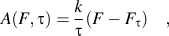 $$A(F,{\rm{\tau }}) = {k \over {\rm{\tau }}}\left( {F - {F_{\rm{\tau }}}} \right)\quad ,$$
where F τ is the minimum load required to produce a maximum shear stress of magnitude τ given by the Hertzian expression shown in Eq. (B7) of Appendix B, and k is a dimensionless constant that depends on Poisson’s ratio ν. The value of the constant k was obtained by fitting the numerically determined areas enclosed in the contours of maximum principal shear stresses for Hertzian elastic contact as a function of Poisson's ratio and is well approximated by
 $$k = 0.022{{\rm{\nu }}^2} - 0.0226{\rm{\nu }} + 0.1245\quad .$$
(a) Schematic representation of the stress distribution in the highly stressed zone showing three representative maximum principal shear stress contours (τ, τa, and τb). The area within the contour of maximum principal shear stress τ is shown as the shaded region, (b) contours of maximum principal shear stress and the differential area element used in the stochastic model. The differential area element ΔA is shaded in gray.
In all further calculations, we will assume ν = 0.3 for which k = 0.1194.
Based on the area of the highly stressed zone in Fig. 5(a), the probability of pop-in at an applied load F can be estimated using weak-link principles as shown schematically in Fig. 5(b). For the dislocation arrangement shown there, which includes randomness in spatial location and spatial orientation, pop-in will occur by dislocation activation if at least one dislocation inside the highly stressed zone can be activated, i.e., if the “resolved” shear stress τr at the location of the dislocation inside the zone is greater than the stress needed to activate it, τcrss. Hence, the probability of pop-in at a given load p(F) depends not only on the probability of finding a dislocation inside the zone but also on the probability p act that the local resolved shear stress is sufficient to activate it. Since the stress field inside the zone is not uniform, we discretize it into N small equal area elements, each having an area ΔA (see Fig. 6) given by
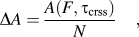 $$\Delta A = {{A\left( {F,{{\rm{\tau }}_{{\rm{crss}}}}} \right)} \over N}\quad ,$$
where A(F, τcrss) is the area enclosed within the maximum principal shear stress contour of τcrss at a load F obtained by substituting τ = τcrss into Eq. (1a). We let j denote an integer incremental variable that varies from 1 to N and is used to increment the areas inside the τcrss contour from ΔA to A(F, τcrss). When j = N, τ = τcrss and the enclosed area inside the τcrss contour is equal to A(F, τcrss). The probability of activating at least one dislocation within the infinitesimal area element ΔA can then be integrated inside the zone up to the boundary [which has an area A(F, τcrss)] to estimate the probability of pop-in, p(F), at a given load F. Following the procedure outlined in Appendix C, this gives
 $$p(F) = 1 - \exp \left( { - {\rm{\rho }}{{A\left( {F,{{\rm{\tau }}_{{\rm{crss}}}}} \right)} \over N}\mathop {\lim }\limits_{N \to \infty } \mathop\sum\limits_{j = 1}^N {{p_{{\rm{act}}}}} } \right)\quad ,$$
which provides the generic framework needed to estimate the probability of pop-in for any type of probability distribution for dislocation activation, p act. Note that the probability calculated using Eq. (3) is the cumulative probability, i.e., the probability of pop-in up to a load F. This follows from the fact that the derivation of Eq. (3) involves a summation of the pop-in probabilities of all the infinitesimal area elements inside the τcrss contour (highly stressed zone) at an applied load F. It should also be noted that for large indenter radii, one would expect the pop-in displacement burst caused by the activation of a preexisting dislocation to become less distinct and eventually experimentally indistinguishable from a smooth elastic–plastic transition.
Case 1: model predictions (solid lines) for the indenter radius dependence of the average maximum shear stress at pop-in. The model is compared with the average of 20,000 Monte Carlo simulation results at a dislocation density of 0.5 µm−2 (filled circles).
To this point, the discussion has been limited to pop-in by activation of preexisting dislocations. However, if pop-in does not occur up to a load F theo at which a maximum shear stress equal to the theoretical strength is generated, then pop-in will occur by the nucleation of dislocations at the theoretical strength. Considering that pop-in may take place by either process, the average pop-in load F avg can be estimated as a weighted average of the pop-in probabilities at various loads [Eq. (3)]. This gives
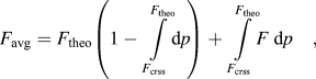 $${F_{{\rm{avg}}}} = {F_{{\rm{theo}}}}\left( {1 - \int\limits_{{F_{{\rm{crss}}}}}^{{F_{{\rm{theo}}}}} {{\rm{d}}p} } \right) + \int\limits_{{F_{{\rm{crss}}}}}^{{F_{{\rm{theo}}}}} {F\;{\rm{d}}p} \quad ,$$
where the first term corresponds to pop-in by dislocation nucleation and the second term corresponds to activation of a preexisting dislocation. In this equation, F theo and F crss can be determined by substituting τtheo and τcrss into Eq. (B7) of Appendix B.
The generic framework developed here can be applied to different situations for the required dislocation activation stress by estimating the corresponding probability of activation p act. In this work, we focus on two such cases. In case 1, all the dislocations are assumed to be favorably oriented relative to the direction of maximum principal shear stress so that randomness in dislocation orientation is not a factor, and only the randomness in spatial location is important. In case 2, the dislocations are assumed to be both randomly located and randomly oriented so that both factors play a role. Although the latter case is more realistic, a great deal of the controlling physics is embodied in the former, which is also easier to describe in closed mathematical form.
B. Case 1: All dislocations are favorably oriented relative to the maximum principal shear stress
Under the condition that all the dislocations are favorably oriented relative to the direction of maximum principal shear stress, any dislocation inside the highly stressed zone will be activated, i.e., the resolved shear stress acting on each of the dislocations inside the zone is always greater than τcrss and hence the probability of activation is p act = 1. Substituting p act = 1 into Eq. (3), the average pop-in load F avg can be determined in a closed form using Eq. (4) and is given by
 $${F_{{\rm{avg}}}} = {F_{{\rm{crss}}}} + {{{{\rm{\tau }}_{{\rm{crss}}}}} \over {{\rm{\rho }}k}}\left\{ {1 - {\rm exp}\left[ { - {{{\rm{\rho }}k} \over {{{\rm{\tau }}_{{\rm{crss}}}}}}\left( {{F_{{\rm{theo}}}} - {F_{{\rm{crss}}}}} \right)} \right]} \right\}\quad ,$$
where F crss and F theo are calculated as explained earlier. The average pop-in load can now be substituted into the Hertzian expression for τmax
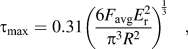 $${{\rm{\tau }}_{{\rm{max}}}} = 0.31{\left( {{{6{F_{{\rm{avg}}}}E_{\rm{r}}^2} \over {{{\rm{\pi }}^3}{R^2}}}} \right)^{{1 \over 3}}}\quad ,$$
to give the average maximum shear stress at pop-in.Reference Shim, Bei, George and Pharr16 The value of τmax computed in this way is a measure of the stress needed to initiate dislocation plasticity. Note that for the limiting cases of low (ρ → 0) and high (ρ → ∞) dislocation density, the model correctly predicts the maximum shear stresses at pop-in as τtheo and τcrss, respectively.
Figure 6 shows a comparison of the average maximum shear stress at pop-in determined by the model along with 20,000 Monte Carlo simulations using E = 100 GPa, τtheo = 10 GPa, and τcrss = 1 GPa. With increasing indenter radius, the maximum shear stress at pop-in transitions from a high strength level (τtheo) to a lower strength level (τcrss), which is precisely the size effect observed in spherical indentation by Shim et al.Reference Shim, Bei, George and Pharr16 and Morris et al.Reference Morris, Bei, Pharr and George23 The Monte Carlo results also confirm the applicability of Eq. (5).
C. Case 2: Dislocations are randomly oriented relative to the direction of maximum principal shear stress
The geometry for case 2 is shown in Fig. 7(a), wherein the edge dislocations are oriented at random angles with respect to the direction of the maximum principal shear stress τ. To define this orientation, we let the dislocation be rotated counterclockwise through an angle α (α is a random angle between 0 and 360°) with respect to the r-axis of the specimen, and we let the direction of the maximum principal shear stress be at a counterclockwise rotation angle θ relative to the r-axis of the specimen [see Fig. 7(a)]. For the dislocation to be activated within the j th contour of maximum principal shear stress τ j, the resolved shear stress acting to move it on its glide plane should be greater than τcrss. This resolved shear stress is given byReference Dieter34
 $${{\rm{\tau }}_{\rm{r}}} = {{\rm{\tau }}_j}\rm cos2({\rm{\theta }} - {\rm{\alpha }})\quad .$$
(a) Schematic of a random orientation of dislocations relative to the direction of maximum principal shear stress and (b) the distribution of the angle (θ) of the maximum principal shear stress relative to the r-axis along contours of maximum principal shear stress.
Figure 7(b) shows the distribution of the angles of maximum principal shear stress (θ) along the contours of maximum principal shear stress for Hertzian elastic contact, from which it follows that θ generally varies from 0 to 45° and from 65 to 90°. As noted earlier, α is a random angle between 0 and 360° and (θ − α) is a random angle that can be calculated by taking the extremes of θ (0 and 360°) and α (0 and 90°). Hence, (θ − α) should be a random angle between −90° (0–90°) and 360° (360–0°). For the dislocation to be activated, the resolved shear stress τr must be greater than τcrss. The probability of such an event, as outlined in Appendix D, is given by
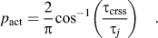 $${p_{{\rm{act}}}} = {2 \over {\rm{\pi }}}{\cos ^{ - 1}}\left( {{{{{\rm{\tau }}_{{\rm{crss}}}}} \over {{{\rm{\tau }}_j}}}} \right)\quad .$$
Substituting the above into Eq. (3), we obtain the probability of pop-in that can be used to calculate the average pop-in load (F avg) using Eq. (4). However, unlike case 1, the average pop-in load cannot be written in a closed form and must be computed numerically from the governing equations.
Figure 8 shows the average maximum shear stress at pop-in for case 2 determined by the model and 20,000 Monte Carlo trials using E =100 GPa, τtheo = 10 GPa, and τcrss = 1 GPa. Similar to case 1 (Fig. 6), there is perfect agreement between the model and the Monte Carlo results, with the shear stress transitioning from a higher strength level (τtheo) to a lower strength level (τcrss) with increasing indenter radius. The figure also shows for comparison the model results for case 1. It is interesting to note that the model predictions for case 2 are in fact very close to those for case 1, implying that most of the stochastic behavior is embodied in the randomness in spatial location alone. Thus, the simple closed form of Eq. (5) is a reasonable first-order estimate of the expected behavior.
Comparison of model predictions for case 1 and case 2. Also shown for case 2 are Monte Carlo simulation results.
D. Scatter in the maximum shear stress at pop-in
One can also use the approach developed here to estimate the amount of scatter that would be expected in the data and how it would vary with material and geometric parameters. To this end, we estimate the scatter in maximum shear stress at pop-in using the approach developed for uniaxial tension/compression data by Sudharshan Phani et al.Reference Sudharshan Phani, Johanns, George and Pharr26 As in the previous work, we model the scatter bounds by the limiting maximum shear stress values within which a given percentage of the maximum shear stresses at pop-in lie. For example, 90% scatter bounds (the bounds that will be used this paper) exclude the top and bottom 5% of the maximum shear stresses but include the middle 90%. Details on how these scatter bounds are calculated are given elsewhere.Reference Sudharshan Phani, Johanns, George and Pharr26
Figure 9(a) shows the 90% scatter bounds for maximum shear stress at pop-in predicted for case 1 using E =100 GPa, τtheo = 10 GPa, and τcrss = 1 GPa. Results of 100 Monte Carlo trials at several discrete indenter radii are also shown for comparison. It is evident from the plot that the model accurately captures the scatter bounds predicted by the Monte Carlo calculations. In addition, similar to the results for average maximum shear stress at pop-in shown in Fig. 8, Fig. 9(b) shows that the scatter bounds for cases 1 and 2 are also very close, with the results for case 2 slightly shifted to the right of case 1. Like the trends observed in uniaxial testing, the scatter is minimal at the extremes of the length scale while it is large at intermediate values. However, unlike the model for uniaxial testing, the scatter in the transition regime is not so concentrated at the extreme values. Thus, the nonuniformity of stress in the highly stressed zone tends to produce pop-in stresses for which the scatter is more uniformly distributed.
(a) Comparison for case 1 of the model predictions for 90% scatter bounds with Monte Carlo results for the maximum shear stress at pop-in and (b) comparison of the model predictions for 90% scatter bounds for case 1 and case 2.
III. COMPARISON WITH EXPERIMENTAL RESULTS
Last, we wish to compare the maximum shear stresses at pop-in predicted by the model for case 1 [Eq. (5)] to the experimental pop-in data for molybdenum single crystals reported by Morris et al.Reference Morris, Bei, Pharr and George23 The inputs required for the model are the theoretical strength (τtheo), the critical resolved shear stress (τcrss), the dislocation density (ρ), and the elastic constants (E and ν). The elastic constants used in the calculations are the same as those used by Morris et al.,Reference Morris, Bei, Pharr and George23E = 327 GPa and ν = 0.3, and for the dislocation density, we assume ρ = 1011 m−2 based on recent x-ray line broadening measurements of the same Mo single crystal by Barabash.Reference Barabash35 Since the current model does not consider scatter in the theoretical strength (this could be added by considering nucleation to be a stress-assisted, thermally activated process as in the recent analysis of Li et al.Reference Li, Bei, Morris, George and Gao25), the value τtheo = 15.9 GPa was used based on the average strength measured at the smallest indenter radius [see Fig. 2(a)]. This is very close to the 15 GPa value predicted by Ogata et al.Reference Ogata, Li, Hirosaki, Shibutani and Yip36 using first principles calculations. Similarly, τcrss was taken as 0.4 GPa based on the average strength for the largest indenter radius. To compare the model to the “cumulative” probability of pop-in as a function of the maximum shear stress at pop-in, as in the original data set presented by Morris et al.,Reference Morris, Bei, Pharr and George23 the cumulative probability given in Eq. (3) can be written in terms of the maximum shear stress at pop-in for case 1 as:
 $$p({{\rm{\tau }}_{\rm max}}) = \,\,1 - {\rm exp}\left( { - {{{\rm{\rho }}k{{\rm{\pi }}^3}{R^2}} \over {0.1787{{\rm{\tau }}_{{\rm{crss}}}}E_{\rm{r}}^2}}\left( {{\rm{\tau }}_{\rm max}^3 - {\rm{\tau }}_{{\rm{crss}}}^3} \right)} \right)\quad {\rm{for }}\;{{\rm{\tau }}_{{\rm{max}}}}{\rm{ \lt }}{{\rm{\tau }}_{{\rm{theo}}}}\quad ,$$
 $$p({\tau _{\rm max}}) = 1\quad {\rm{for\; }}{{\rm{\tau }}_{{\rm{max}}}} = {{\rm{\tau }}_{{\rm{theo}}}}\quad .$$
Figure 10 compares the experimental data to the case 1 model predictions [Eq. (9)] plotted as the cumulative probability of pop-in versus maximum shear stress τmax for each indenter radius R, where the indenter radius (in micrometre) is shown beside the corresponding curve. Generally, good agreement between the model predictions and the experimental data is observed over the entire range of indenter radii. Figure 11 replots the data as τmax at pop-in versus R to assess the 90% scatter band predicted by the model. The plot shows that the model adequately captures the magnitude of the scatter, with the scatter being largest at the intermediate indenter radii and smallest at the extremes of R. Although we cannot categorically rule out that the experimental data are uninfluenced by surface hardening during polishing by oxide surface layers, or by surface roughness, the fact that the new model fits so well to the experimental data with essentially no adjustable parameters gives us some confidence that surface effects do not play a major role. This is also to be expected based on the care that was taken in preparing the specimen.Reference Morris, Bei, Pharr and George23 It is thus clear that the current approach can be used to reconcile the experimentally observed indenter size effects in pop-in from a purely statistical point of view.
Comparison of experimental data (open circles) for the cumulative probability of pop-in in Mo as a function of the maximum shear stress at pop-in (Morris et al.Reference Morris, Bei, Pharr and George23) with our model predictions for case 1 (solid lines). The indenter radius (in μm) is shown beside the corresponding curve.
Comparison of experimental data for the maximum shear stress at pop-in in single crystal Mo (Morris et al.Reference Morris, Bei, Pharr and George23) with model predictions (case 1) for 90% scatter bounds.
IV. SUMMARY AND CONCLUSIONS
A weak-link statistical model has been developed to predict the pop-in loads and maximum shear stress at pop-in as a function of indenter radius. The model predicts the cumulative probability of pop-in as a function of maximum shear stress at pop-in in simple closed form for the case of randomly spaced dislocations. The model considers pop-in resulting from both the nucleation of dislocations and the activation of preexisting dislocations. The model predicts a transition in the maximum shear stress at pop-in from a higher strength level (τtheo) to a lower strength level (τcrss) with increasing indenter radius, thus explaining recently reported experimental observations for Ni and Mo single crystals. The model also accurately captures the scatter in the Mo single crystal data. The results closely follow the “size effect” trends observed in microcompression and tension testing and point to the important role played by stochastic processes in determining strength at small length scales.
ACKNOWLEDGMENT
This work was supported by the U.S. Department of Energy, Office of Basic Energy Sciences, Materials Sciences and Engineering Division.
APPENDIX A: Elastic stress field under a spherical indenter at an applied load F
For an isotropic elastic material with Young’s modulus E and Poisson’s ratio ν, the stress components in a cylindrical coordinate system (r, θ, z) for indentation by a spherical indenter with radius, R, and contact radius, a, are given byReference Fischer-Cripps32,Reference Huber33
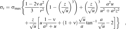 $$\eqalignb{ {\rm{\sigma }}_{\rm{r}} = {\rm{\sigma }}_{\max } \left\{ {{{1 - 2{\rm{\nu }}} \over 3}{{a^2 } \over {r^2 }}\left( {1 - \left( {{z \over {\sqrt u }}} \right)^3 } \right) + \left( {{z \over {\sqrt u }}} \right)^3 {{a^2 u} \over {u^2 + a^2 z^2 }}} \right. \cr {\rm{ }}\left. { + {z \over {\sqrt u }}\left[ {u{{1 - {\rm{\nu }}} \over {a^2 + u}} + \left( {1 + {\rm{\nu }}} \right){{\sqrt u } \over a}\tan ^{ - 1} {a \over {\sqrt u }} - 2} \right]} \right\}\quad , \cr} $$
 $${{\rm{\sigma }}_z} = - {{\rm{\sigma }}_{\max }}{\left( {{z \over {\sqrt u }}} \right)^3}{{{a^2}u} \over {{u^2} + {a^2}{z^2}}}\quad ,$$
 $${{\rm{\tau }}_{rz}} = - {{\rm{\sigma }}_{\max }}\left( {{{r{z^2}} \over {{u^2} + {a^2}{z^2}}}} \right)\left( {{{{a^2}\sqrt u } \over {{a^2} + u}}} \right)\quad ,$$
where
 $$u = {\textstyle{1 \over 2}}\{ ({r^2} + {z^2} - {a^2}) + {[{({r^2} + {z^2} - {a^2})^2} + 4{a^2}{z^2}]^{1/2}}\}\quad.$$
Other important relations are
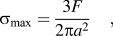 $${{\rm{\sigma }}_{\max }} = {{3F} \over {2{\rm{\pi }}{a^2}}}\quad ,$$
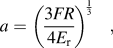 $$a = {\left( {{{3FR} \over {4{E_{\rm{r}}}}}} \right)^{{1 \over 3}}}\quad ,$$
and
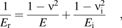 $${1 \over {{E_{\rm{r}}}}} = {{1 - {{\rm{\nu }}^2}} \over E} + {{1 - {\rm{\nu }}_{\rm{i}}^2} \over {{E_{\rm{i}}}}}\quad ,$$
where E i and E are the moduli of the indenter and specimen and νi and ν are their Poisson's ratios, respectively.
The maximum principal shear stress (τmax) and the corresponding angle (θ) that it makes with the r-axis [see Fig. 7(a)] can be calculated from these equations using Mohr's circle concepts. They are given byReference Dieter34
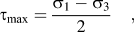 $${{\rm{\tau }}_{\rm max}} = {{{{\rm{\sigma }}_1} - {{\rm{\sigma }}_3}} \over 2}\quad ,$$
where
 $${{\rm{\sigma }}_{1,3}} = {{{{\rm{\sigma }}_r} + {{\rm{\sigma }}_z}} \over 2} \pm {\left[ {{{\left( {{{{{\rm{\sigma }}_r} - {{\rm{\sigma }}_z}} \over 2}} \right)}^2} + {\rm{\tau }}_{rz}^2} \right]^{1/2}}\quad ,$$
and
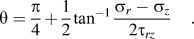 $${\rm{\theta }} = {{\rm{\pi }} \over 4} + {1 \over 2}{\tan ^{ - 1}}{{{{\rm{\sigma }}_r} - {{\rm{\sigma }}_z}} \over {2{{\rm{\tau }}_{rz}}}}\quad .$$
APPENDIX B: Area enclosed within a maximum principal shear stress contour
The area enclosed within a maximum principal shear stress contour, τ, as schematically shown by the shaded region in Fig. 5, can be determined by dimensional analysis. Let the spatial coordinates be normalized by the contact radius, a, and the stress components by the elastic modulus, E, such that
 $$\overline r = {r \mathord{\left/ {\vphantom {r a}} \right. \kern-\nulldelimiterspace} a}\quad {\rm{and}}\quad \overline z = {z \mathord{\left/ {\vphantom {z a}} \right. \kern-\nulldelimiterspace} a}\quad ,$$
where the bars over the symbols (e.g.,  $\bar r,\bar z$) represent the nondimensional quantities. The enclosed area, A, within a maximum principal shear stress contour can then be nondimensionalized as
 $$\overline A = {A \mathord{\left/ {\vphantom {A {a^2 }}} \right. \kern-\nulldelimiterspace} {a^2 }}\quad ,$$
and the stress components shown in Appendix A can be rewritten in nondimensional form as
 $$\overline {{{\rm{\sigma }}_r}} ,\overline {{{\rm{\sigma }}_z}} ,\overline {{{\rm{\tau }}_{rz}}} ,\overline {\rm{\tau }} = {{{{\rm{\sigma }}_{\max }}} \over E}f\left( {\overline r ,\overline z ,{\rm{\nu }}} \right){\rm{ }}\quad {\rm{.}}$$
Hence,
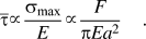 $$\overline {\rm{\tau }} \propto {{{{\rm{\sigma }}_{\max }}} \over E} \propto {F \over {{\rm{\pi }}E{a^2}}}\quad .$$
From Eqs. (B2) and (B4), the maximum principal shear stress can be written as
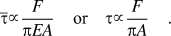 $$\overline {\rm{\tau }} \propto {F \over {{\rm{\pi }}EA}}\quad {\rm{or}}\quad {\rm{\tau }} \propto {F \over {{\rm{\pi }}A}}\quad .$$
Thus, for a maximum principal shear stress contour of τ (see Fig. 5), the enclosed area can be written as
 $${\rm{\tau }} = k{{F - {F_{\rm{\tau }}}} \over A}\quad {\rm{or}}\quad A\left( {F,{\rm{\tau }}} \right) = k{{F - {F_{\rm{\tau }}}} \over {\rm{\tau }}}\quad ,$$
where k is a proportionality constant that is a function of Poisson's ratio ν, and F τ is the minimum load required to generate a maximum shear stress of τ in the specimen. The value of F τ can be determined from Hertzian elastic contact theory through the following relation:
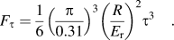 $${F_{\rm{\tau }}} = {1 \over 6}{\left( {{{\rm{\pi }} \over {0.31}}} \right)^3}{\left( {{R \over {{E_{\rm{r}}}}}} \right)^2}{{\rm{\tau }}^3}\quad .$$
The value of the constant k can be obtained by fitting the numerically determined areas enclosed in the contours of maximum principal shear stresses for Hertzian elastic contact as a function of Poisson's ratio. It is well approximated by Eq. (1b)
 $$k = 0.022{\nu ^2} - 0.0226\nu + 0.1245\quad .$$
APPENDIX C: Probability of pop-in due to activation of preexisting dislocations
In the proposed weak-link model [see Fig. 5(b)], pop-in occurs by activation of dislocations at a load F if at least one dislocation is activated within the τcrss contour. Let the specimen have n dislocations randomly oriented and spaced. The probability of at least one dislocation being activated is one minus the probability that none of the dislocations are activated. For dislocations not to be activated within the τcrss contour, either there should be no dislocations within the contour or the shear stress acting on the dislocations should be lower than their activation stress. This probability p(F) can be written as follows:
 $$\eqalignb{ p(F) = 1 - [p({\rm{no \;dislocations\; within\; \tau }}_{{\rm{crss}}}\; {\rm{ contour}}) \cr \;\;\;\;\;\; + \forall \;{\rm{dislocations\; within\; \tau }}_{{\rm{crss}}}\; {\rm{ contour\!\!: \;}}p({\rm{\tau }}_{\rm{r}} \lt {\rm{\tau }}_{{\rm{crss}}} )]\quad . \cr} $$
Note that for a given dislocation
 $$p\left( {{\tau _{\rm{r}}} \lt {\tau _{{\rm{crss}}}}} \right) = 1 - {p_{{\rm{act}}}}\quad ,$$
where p act is the probability of activation.
To calculate the probability that no dislocations are activated within the τcrss contour, the area inside the τcrss contour can be discretized into N smaller equal-area elements of area ΔA [see Fig. 5(b)]. The probabilities of no dislocations being activated within each area element can then be multiplied to obtain the probability of no dislocations being activated within the entire τcrss contour.
For a specimen having n dislocations (n → ∞) with a dislocation density ρ, the probability of finding i dislocations within an area is given byReference Sudharshan Phani, Johanns, George and Pharr26
 $$p(i) = {{\rm{e}}^{ - {\rm{\rho }}\Delta A}}{{{{\left( {{\rm{\rho }}\Delta A} \right)}^i}} \over {(i)!}}\quad .$$
Hence, the probability that there are no dislocations within an area ΔA is
 $$p(0) = {{\rm{e}}^{ - {\rm{\rho }}\Delta A}}\quad .$$
The probability that none of the dislocations within the infinitesimal area elements ΔA are activated can then be written as
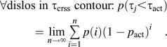 $$\forall {\rm{dislos \;in }}\;{{\rm{\tau }}_{{\rm{crss}}}}\;{\rm{ contour\!\!: }}\;p({{\rm{\tau }}_j} \lt {{\rm{\tau }}_{{\rm{act}}}}) = \mathop {\lim }\limits_{n \to \infty } \mathop \sum\limits_{i = 1}^n {p(i){{(1 - {p_{{\rm{act}}}})}^i}} \quad .$$
Substituting Eqs. (C4) and (C5) in Eq. (C1) and multiplying the probabilities of all the area elements (1 to N), we obtain
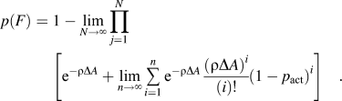 $$p(F) = \;1 - \mathop {\lim }\limits_{N \to \infty } \prod\limits_{j = 1}^N {\left[ {{{\rm{e}}^{ - {\rm{\rho }}\Delta A}} + \mathop {\lim }\limits_{n \to \infty } \mathop \sum\limits_{i = 1}^n {{{\rm{e}}^{ - {\rm{\rho }}\Delta A}}{{{{\left( {\rho \Delta A} \right)}^i}} \over {(i)!}}} {{\left( {1 - {p_{{\rm{act}}}}} \right)}^i}} \right]} \quad .$$
The above equation can be simplified to
 $$p(F) = 1 - \exp \left( { - {\rm{\rho }}{{A\left( {F,{{\rm{\tau }}_{{\rm{crss}}}}} \right)} \over N}\mathop {\lim }\limits_{N \to \infty } \mathop \sum\limits_{j = 1}^N {{p_{{\rm{act}}}}} } \right)\quad .$$
APPENDIX D: Probability of activation (p act) of preexisting dislocations randomly oriented relative to the direction of maximum principal shear stress (case 2)
For the dislocation to be activated within the j th contour of maximum principal shear stress τj, the resolved shear stress acting to move it on its glide plane should be greater than τcrss. The probability of such an event can be written using Eq. (7) as
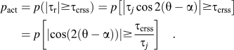 $${p_{{\rm{act}}}} = p\left( {\left| {{{\rm{\tau }}_{\rm{r}}}} \right| \ge {{\rm{\tau }}_{{\rm{crss}}}}} \right) = p\left[ {\left| {{{\rm{\tau }}_j}\cos 2\left( {{\rm{\theta }} - {\rm{\alpha }}} \right)} \right| \ge {{\rm{\tau }}_{{\rm{crss}}}}} \right] = p\left[ {\left| {\cos \left( {2\left( {{\rm{\theta }} - {\rm{\alpha }}} \right)} \right)} \right| \ge {{{{\rm{\tau }}_{{\rm{crss}}}}} \over {{\tau _j}}}} \right]\quad .$$
The absolute value of the resolved shear stress is used in this analysis as the activation depends only on the magnitude of the shear stress.
The probability of activation p act can then be calculated as the ratio of the range of angles that satisfy the condition, |cos[2(θ − α)]| ≥ τcrss/τj to the total range of angles for 2(θ − α), which is 5π (−π to 4π). Since the cosine function is cyclical and its absolute value is of interest in the present case, we can calculate the range of angles that satisfy the above inequality for a smaller range such as 0 to π and then extend it to the total range (−π to 4π) by multiplying by 5. The range of angles between 0 and π that satisfy the condition |cos[2(θ − α)]| ≥ τcrss/τj is 2θ*, where θ* = cos−1(τcrss/τj). Hence, the probability of activation for the entire range of angles is
 $${p_{{\rm{act}}}} = {{2{{\rm{\theta }}^*} \times 5} \over {4{\rm{\pi }} - ( - {\rm{\pi }})}} = {{2{{\rm{\theta }}^*}} \over {\rm{\pi }}} = {2 \over {\rm{\pi }}}{\cos ^{ - 1}}\left( {{{{{\rm{\tau }}_{{\rm{crss}}}}} \over {{{\rm{\tau }}_j}}}} \right)\quad .$$



