


1 Introduction
Let
 $\unicode[STIX]{x1D6EC}:=\operatorname{SL}_{2}(\mathbf{Z})$
be the modular group. Then
 $\unicode[STIX]{x1D6EC}$
acts on the hyperbolic upper half plane
 $\mathbb{H}$
by Möbius transformations and the quotient
 $X:=\unicode[STIX]{x1D6EC}\backslash \mathbb{H}$
is an orbifold Riemann surface. We denote by
 $\unicode[STIX]{x1D6EC}(q)$
the principal congruence subgroup of
 $\unicode[STIX]{x1D6EC}$
given by the kernel of the reduction modulo
 $q$
map
 $\unicode[STIX]{x1D6EC}\rightarrow \operatorname{SL}_{2}(\mathbf{Z}/q\mathbf{Z})$
. Then
 $\unicode[STIX]{x1D6EC}(q)$
is a normal subgroup of
 $\unicode[STIX]{x1D6EC}$
and for
 $q\geqslant 2$
 $$\begin{eqnarray}\displaystyle X(q):=\unicode[STIX]{x1D6EC}(q)\backslash \mathbb{H} & & \displaystyle \nonumber\end{eqnarray}$$
is a Riemann surface.
If we parameterize points in
 $\mathbb{H}$
by
 $x+iy$
with
 $x,y\in \mathbf{R}$
and
 $y>0$
, then the Laplacian on
 $\mathbb{H}$
is given by
 $$\begin{eqnarray}\displaystyle \unicode[STIX]{x1D6E5}=-y^{2}\biggl(\frac{\unicode[STIX]{x2202}^{2}}{\unicode[STIX]{x2202}x^{2}}+\frac{\unicode[STIX]{x2202}^{2}}{\unicode[STIX]{x2202}y^{2}}\biggr). & & \displaystyle \nonumber\end{eqnarray}$$
This operator is invariant under Möbius transformations and hence descends to an operator on smooth functions on
 $X(q)$
. The surface
 $X(q)$
also has a measure
 $\unicode[STIX]{x1D707}_{q}$
induced from the
 $\unicode[STIX]{x1D6EC}$
-invariant volume form
 $(dx\wedge dy)/y^{2}$
on
 $\mathbb{H}$
. The Laplacian extends to an unbounded operator
 $\unicode[STIX]{x1D6E5}_{X(q)}$
on
 $L^{2}(X,\unicode[STIX]{x1D707}_{q})$
. For all
 $q\geqslant 2$
,
 $\unicode[STIX]{x1D6E5}_{X(q)}$
has a simple eigenvalue at 0 and the spectrum of
 $\unicode[STIX]{x1D6E5}_{X(q)}$
below
 $\frac{1}{4}$
is discrete. Therefore we may write
 $\unicode[STIX]{x1D706}_{1}(X(q))$
for the smallest non-zero eigenvalue of
 $\unicode[STIX]{x1D6E5}_{X(q)}$
. In a celebrated 1965 paper [Reference SelbergSel65], Selberg proved the following.
Theorem 1.1 (Selberg’s
 $\frac{3}{16}$
theorem).

For all
 $q\geqslant 2$
,
 $\unicode[STIX]{x1D706}_{1}(X(q))\geqslant \frac{3}{16}$
.
At the same time, Selberg made the following conjecture.
Conjecture 1.2 (Selberg’s eigenvalue conjecture).
For all
 $q\geqslant 2$
,
 $\unicode[STIX]{x1D706}_{1}(X(q))\geqslant \frac{1}{4}$
.
This conjecture cannot be pushed any further since there are examples [Reference MaassMaa49] of
 $q$
such that
 $\unicode[STIX]{x1D6E5}_{X(q)}$
has an eigenvalue at
 $\frac{1}{4}$
. Progress on Conjecture 1.2 has been made by several authors over the interim decades, including works of Gelbart and Jacquet (
 $\unicode[STIX]{x1D706}_{1}>\frac{3}{16}$
) [Reference Gelbart and JacquetGJ78], Luo, Rudnick and Sarnak (
 $\unicode[STIX]{x1D706}_{1}\geqslant \frac{171}{784}$
) [Reference Luo, Rudnick and SarnakLRS95], and Iwaniec (
 $\unicode[STIX]{x1D706}_{1}\geqslant \frac{10}{49}$
) [Reference IwaniecIwa96]. The current best result is due to Kim and Sarnak [Reference KimKim03] who proved for all
 $q\geqslant 2$
,
 $$\begin{eqnarray}\displaystyle \unicode[STIX]{x1D706}_{1}(X(q))\geqslant {\textstyle \frac{975}{4096}}\approx 0.238. & & \displaystyle \nonumber\end{eqnarray}$$
Selberg’s conjecture remains one of the fundamental open questions of automorphic forms; see the expository articles of Sarnak [Reference SarnakSar95, Reference SarnakSar05].
Selberg’s conjecture can also be stated in terms of representation theory. This is fitting with Selberg’s original motivationFootnote
1
of Conjecture 1.2 as an archimedean analog of the Ramanujan–Petersson conjectures. The equivalence classes of irreducible unitary representations (unitary dual) of
 $\operatorname{SL}_{2}(\mathbf{R})$
were classified by Bargmann [Reference BargmannBar47]: one has the trivial representation, the principal series, complementary series, discrete series and limits of discrete series. Of particular interest to us are the complementary series
 $\operatorname{Comp}^{u}$
that are indexed by a parameter
 $u\in (0,1)$
; see [Reference KnappKna01, p. 36] for a precise description of these representations.
For each
 $q\geqslant 2$
, we obtain a unitary representation of
 $\operatorname{SL}_{2}(\mathbf{R})$
on
 $L^{2}(\unicode[STIX]{x1D6EC}(q)\backslash \operatorname{SL}_{2}(\mathbf{R}))$
by right translation. This representation can be decomposed as a direct integral over a projection-valued measure on the unitary dual of
 $\operatorname{SL}_{2}(\mathbf{R})$
. Conjecture 1.2 is equivalent to the following.
Conjecture 1.2*.
For all
 $q\geqslant 2$
, the measure on the unitary dual of
 $\operatorname{SL}_{2}(\mathbf{R})$
that decomposes
 $L^{2}(\unicode[STIX]{x1D6EC}(q)\backslash \operatorname{SL}_{2}(\mathbf{R}))$
is supported away from complementary series representations.
The point of view taken in this work is that
 $\unicode[STIX]{x1D6EC}\backslash \operatorname{SL}_{2}(\mathbf{R})$
is the moduli space of unit area translation surfaces of genus 1 and hence Selberg’s eigenvalue conjecture is a conjecture about moduli spaces and their covering spaces. A translation surface is a closed topological surface
 $S$
with a finite subset
 $\unicode[STIX]{x1D6F4}$
, together with a set of complex charts on
 $S-\unicode[STIX]{x1D6F4}$
such that all transition functions are translations, and the charts extend to conical singularities at
 $\unicode[STIX]{x1D6F4}$
. Let
 $\unicode[STIX]{x1D6F4}=\{A_{1},\ldots ,A_{s}\}$
. The conical singularity at
 $A_{i}$
is required to have cone angle
 $2\unicode[STIX]{x1D70B}(\unicode[STIX]{x1D705}_{i}+1)$
with
 $\unicode[STIX]{x1D705}_{i}\in \mathbf{Z}_{+}$
and the Gauss–Bonnet theorem forces the relation
 $$\begin{eqnarray}\displaystyle \mathop{\sum }_{i=1}^{s}\unicode[STIX]{x1D705}_{i}=2g-2. & & \displaystyle \nonumber\end{eqnarray}$$
Translation surfaces can be equivalently be thought of as abelian differentials with respect to a complex structure on
 $S$
. The zeros of the differential correspond to the conical singularities of the translation surface.
The moduli space of translation surfaces of genus
 $g\geqslant 2$
is stratified according to the partitions
 $\unicode[STIX]{x1D705}=(\unicode[STIX]{x1D705}_{1},\ldots ,\unicode[STIX]{x1D705}_{s})$
. A stratum
 ${\mathcal{H}}(\unicode[STIX]{x1D705})$
need not be connected, but there are finitely many connected components that are understood by work of Kontsevich and Zorich [Reference Kontsevich and ZorichKZ03]. We let
 ${\mathcal{H}}^{(1)}(\unicode[STIX]{x1D705})\subset {\mathcal{H}}(\unicode[STIX]{x1D705})$
denote the unit area translation surfaces in
 ${\mathcal{H}}(\unicode[STIX]{x1D705})$
. In this paper,
 ${\mathcal{M}}$
will be a connected component of
 ${\mathcal{H}}^{(1)}(\unicode[STIX]{x1D705})$
. Since
 ${\mathcal{H}}^{(1)}(\unicode[STIX]{x1D705})$
can be obtained as a quotient of a Teichmüller space by the mapping class group
 $\unicode[STIX]{x1D6E4}=\unicode[STIX]{x1D6E4}(S,\unicode[STIX]{x1D6F4})$
of
 $(S,\unicode[STIX]{x1D6F4})$
(see § 2.1), we may define congruence covers via the natural family of maps
 $$\begin{eqnarray}\displaystyle \unicode[STIX]{x1D6F1}_{q}:\unicode[STIX]{x1D6E4}\mapsto \operatorname{Aut}(H_{1}(S,\mathbf{Z}/q\mathbf{Z})). & & \displaystyle\end{eqnarray}$$
The principal congruence subgroup
 $\unicode[STIX]{x1D6E4}(q)$
is defined to be the kernel of
 $\unicode[STIX]{x1D6F1}_{q}$
. By considering moduli only up to
 $\unicode[STIX]{x1D6E4}(q)$
, and not
 $\unicode[STIX]{x1D6E4}$
, for each connected component
 ${\mathcal{M}}$
of
 ${\mathcal{H}}^{(1)}(\unicode[STIX]{x1D705})$
we obtain a congruence cover
 ${\mathcal{M}}(q)$
generalizing
 $\unicode[STIX]{x1D6EC}(q)\backslash \operatorname{SL}_{2}(\mathbf{R})$
. The details of this construction are given in § 2.1.
Each component
 ${\mathcal{M}}$
has the following associated objects generalizing those attached to
 $\unicode[STIX]{x1D6EC}\backslash \operatorname{SL}_{2}(\mathbf{R})$
.
– There is an action of
$\operatorname{SL}_{2}(\mathbf{R})$
on
${\mathcal{M}}$
. The restriction of the
$\operatorname{SL}_{2}(\mathbf{R})$
action to the one parameter diagonal subgroup gives a flow on
${\mathcal{M}}$
called the Teichmüller flow that generalizes the geodesic flow on the unit tangent bundle of
$X$
.– There is a unique probability measure
$\unicode[STIX]{x1D708}_{{\mathcal{M}}}$
on
${\mathcal{M}}$
that is
$\operatorname{SL}_{2}(\mathbf{R})$
-invariant, ergodic for the Teichmüller flow, and in the Lebesgue class with respect to a natural affine orbifold structure on
${\mathcal{M}}$
. This is due to works of Masur [Reference MasurMas82] and Veech [Reference VeechVee82].– The space
$\operatorname{SO}(2)\backslash {\mathcal{M}}$
is locally foliated by
$\mathbb{H}$
and hence it is possible to define a foliated Laplacian
$\unicode[STIX]{x1D6E5}_{{\mathcal{M}}}$
on
$\operatorname{SO}(2)\backslash {\mathcal{M}}$
generalizing
$\unicode[STIX]{x1D6E5}_{X}$
. This operator has a simple eigenvalue at zero and by a result of Avila and Gouëzel [Reference Avila and GouëzelAG13] its spectrum below
$\frac{1}{4}$
has no accumulation points other than possibly at
$\frac{1}{4}$
.


Each of these objects lifts to
 ${\mathcal{M}}(q)$
, so there is an
 $\operatorname{SL}_{2}(\mathbf{R})$
action on
 ${\mathcal{M}}(q)$
preserving a finite measure
 $\unicode[STIX]{x1D708}_{{\mathcal{M}}(q)}$
, and a foliated Laplacian
 $\unicode[STIX]{x1D6E5}_{{\mathcal{M}}(q)}$
whose spectrum below
 $\frac{1}{4}$
does not accumulateFootnote
2
away from
 $\frac{1}{4}$
. Hence we can write
 $\unicode[STIX]{x1D706}_{1}({\mathcal{M}}(q))$
for the infimum of the non-zero spectrumFootnote
3
of
 $\unicode[STIX]{x1D6E5}_{{\mathcal{M}}(q)}$
. The following extension of Selberg’s conjecture to genus
 $g\geqslant 2$
was proposed by Yoccoz.Footnote
4
Conjecture 1.3 (Yoccoz).
For all
 $q\geqslant 2$
, and any connected component
 ${\mathcal{M}}$
of a stratum, we have the following:
(A)
$\unicode[STIX]{x1D706}_{1}({\mathcal{M}}(q))\geqslant \frac{1}{4}$
;(B) the measure on the unitary dual of
$\operatorname{SL}_{2}(\mathbf{R})$
that decomposes
$L^{2}({\mathcal{M}}(q),\unicode[STIX]{x1D708}_{{\mathcal{M}}(q)})$
is supported away from complementary series representations.


The main theorem of this paper gives an approximation to Conjecture 1.3.
Theorem 1.4. For any connected component
 ${\mathcal{M}}$
of a stratum, there exists
 $\unicode[STIX]{x1D716},\unicode[STIX]{x1D702}>0$
and
 $Q_{0}$
Footnote
5
 $\in \mathbf{Z}_{+}$
such that for all
 $q$
coprime to
 $Q_{0}$
the following hold:
(A)
$\unicode[STIX]{x1D706}_{1}({\mathcal{M}}(q))\geqslant \unicode[STIX]{x1D716}$
;(B) the measure on the unitary dual of
$\operatorname{SL}_{2}(\mathbf{R})$
that decomposes
$L^{2}({\mathcal{M}}(q),\unicode[STIX]{x1D708}_{{\mathcal{M}}(q)})$
is supported away from complementary series representations
$\operatorname{Comp}^{u}$
with
$u\in (1-\unicode[STIX]{x1D702},1)$
;(C) the Teichmüller flow on
${\mathcal{M}}(q)$
has exponential decay of correlations on compactly supported
$C^{1}$
observables with a rate of decay that is independent of
$q$
.





The corresponding theorem for
 ${\mathcal{M}}$
, i.e. without any congruence aspect, was obtained by Avila, Gouëzel and Yoccoz in [Reference Avila, Gouëzel and YoccozAGY06]. In an earlier version of this manuscript, for certain types of components
 ${\mathcal{M}}$
, Theorem 1.4 was conditional on a conjecture of Zorich [Reference ZorichZor99] that has since been proved by Gutiérrez-Romo [Reference Gutiérrez-RomoGut19].
It is known that parts (A), (B), and (C) of Theorem 1.4 are equivalent. That part (B) implies part (C), namely, that one can use representation theory to deduce rates of mixing of the diagonal flow, is due to Ratner [Reference RatnerRat87]. The argument that part (C) implies part (B) is given by the ‘reverse Ratner estimates’ in [Reference Avila, Gouëzel and YoccozAGY06, Appendix B]. The equivalence between parts (A) and (B) is due to the interpretation of the foliated Laplacian as a Casimir operator. This is discussed in detail in [Reference Avila and GouëzelAG13, § 3.4].
So it is sufficient to prove the dynamical statement of part (C). This is made into a precise statement in Theorem 3.5.
We mention that in recent work [Reference Magee and RührMR19], joint with Rühr and Gutiérrez-Romo, we extend Theorem 1.4 to congruence covers coming from relative homology of
 $(S,\unicode[STIX]{x1D6F4})$
, and apply both Theorem 1.4 and the extended result to the problem of counting saddle connections in a homology class modulo
 $q$
.
The current paper deals with Masur–Veech measures on components of strata of abelian differentials. As pointed out to us by Eskin, one can ask whether the results of the current paper extend to arbitrary
 $\operatorname{SL}_{2}(\mathbf{R})$
-invariant and ergodic probability measuresFootnote
6
on strata. The natural starting point for such an investigation is the paper of Avila and Gouëzel [Reference Avila and GouëzelAG13] where a spectral gap result is obtained for such measures. It is not clear how to combine the methods of the current paper with [Reference Avila and GouëzelAG13], since the methods here make crucial use of a symbolic coding of the Teichmüller flow. On the other hand, the methods of [Reference Avila and GouëzelAG13] are based on anisotropic Sobolev spaces and do not involve a symbolic model.
1.1 The ideas of the proof
The reader is invited to read this section before the rest of the paper for the main ideas of the proof.
While we will prove Theorem 1.4 in dynamical terms, the philosophy of the proof goes back to works of Brooks [Reference BrooksBro86] and Burger [Reference BurgerBur86, Reference BurgerBur88] that were originally stated in terms of the first non-zero eigenvalue
 $\unicode[STIX]{x1D706}_{1}$
. Both Brooks and Burger realized that if one has a Galois covering
 $Y\rightarrow X$
of Riemann surfaces, with deck transformation group
 $G$
, then one can transfer bounds on the spectral gap of the Cayley graph of
 $G$
with respect to certain generators, to bounds on the first non-zero eigenvalue
 $\unicode[STIX]{x1D706}_{1}(Y)$
of the Laplacian on
 $Y$
. In particular, if
 $X$
is fixed, and
 $Y$
ranges over a family of Galois covers, if the associated Cayley graphs have a uniform spectral gap, then
 $\unicode[STIX]{x1D706}_{1}(Y)$
is uniformly bounded below away from zero.
The classic construction of an infinite family of graphs of bounded degree with a uniform spectral gap, known as an expander family, is take a fixed generating set
 $U$
in an arithmetic lattice
 $G(\mathbf{Z})$
that has Kazhdan’s property (T), and then form the Cayley graphs for
 $G(\mathbf{Z}/q\mathbf{Z})$
with respect to the projection of
 $U$
modulo
 $q$
. This construction is due to Margulis [Reference MargulisMar73].
Since the covering spaces
 ${\mathcal{M}}(q)$
of this paper have deck transformation groups contained in
 $\operatorname{Sp}(H_{1}(S,\mathbf{Z}/q\mathbf{Z}),\cap )\cong \operatorname{Sp}_{2g}(\mathbf{Z}/q\mathbf{Z})$
, and
 $\operatorname{Sp}_{2g}(\mathbf{Z})$
has property (T) for
 $g\geqslant 2$
, one might expect the Brooks–Burger philosophy to apply directly here, as long as one can prove that the deck transformation group is all of
 $\operatorname{Sp}_{2g}(\mathbf{Z}/q\mathbf{Z})$
, or in other words,
 ${\mathcal{M}}(q)$
is connected. However even if the issue of
 ${\mathcal{M}}(q)$
being connected is resolved,Footnote
7
the Brooks–Burger philosophy does not obviously apply. The core issue is that the foliated Laplacian is not elliptic and only measures fluctuations of functions in the direction of
 $\operatorname{SL}_{2}(\mathbf{R})$
-leaves.
Instead we take a dynamical viewpoint. We think of functions on
 ${\mathcal{M}}(q)$
as sections of a
 $\operatorname{Sp}_{2g}(\mathbf{Z}/q\mathbf{Z})$
principal bundle over
 ${\mathcal{M}}$
, and make this precise in Lemma 2.1. We know the dynamics on
 ${\mathcal{M}}$
is exponentially mixing by the work of Avila, Gouëzel and Yoccoz [Reference Avila, Gouëzel and YoccozAGY06]. The key point for obtaining uniform exponential mixing as in Theorem 1.4(C) is to exploit the following fact: when one travels along the Teichmüller flow and returns close to the initial point, we move in the fibre by a monodromy element of
 $\operatorname{Sp}_{2g}(\mathbf{Z}/q\mathbf{Z})$
. This monodromy is globally defined in the sense that for a given approximate loop, the monodromy at different levels
 $q$
are obtained by reduction mod
 $q$
of some element of
 $\operatorname{Sp}_{2g}(\mathbf{Z})$
. Moreover, if one can argue that the dynamics on the base
 ${\mathcal{M}}$
is sufficiently combinatorially complicated, then we can obtain many monodromy elements in this way. Then we hope to use property (T) to prove this dynamics in the fibre spreads out exponentially fast. So one has exponential mixing in the base, and some form of exponential mixing in the fibres, and hopes to combine these two. The problem is that the two processes are not independent. So we will use hyperbolicity of the dynamics on the base
 ${\mathcal{M}}$
to ‘decouple’ these aspects of the dynamics. However, the base dynamics is not uniformly hyperbolic, so one needs to perform ‘time acceleration’ as in [Reference Avila, Gouëzel and YoccozAGY06] to induce uniform hyperbolicity and then incorporate this into the method.
The previous paragraph was a high level overview of the approach. Now we give details of how this is implemented.
Our framework for understanding the dynamics of
 ${\mathcal{M}}$
is that same as Avila, Gouëzel and Yoccoz in [Reference Avila, Gouëzel and YoccozAGY06]. Namely, instead of working with
 ${\mathcal{M}}$
, we pass to a finite cover called the moduli space of zippered rectangles
 $\text{Rect}_{{\mathcal{M}}}$
for
 ${\mathcal{M}}$
. This finite cover carries a lift of the Teichmüller flow that has some very nice properties that were worked out in [Reference Avila, Gouëzel and YoccozAGY06]. A key insight of [Reference Avila, Gouëzel and YoccozAGY06] is that by carefully choosing a cross section, one obtains a model of the flow on
 $\text{Rect}_{{\mathcal{M}}}$
as a suspension flow over a hyperbolic skew product
 $\hat{Z}:\hat{\unicode[STIX]{x1D6EF}}\rightarrow \hat{\unicode[STIX]{x1D6EF}}$
with a base transformation
 $Z:\unicode[STIX]{x1D6EF}\rightarrow \unicode[STIX]{x1D6EF}$
that is a uniformly expanding Markoff map (Lemmas 3.2 and Proposition 3.1). Moreover the roof function for this suspension model has desirable properties, it is ‘good’ in the sense of [Reference Avila, Gouëzel and YoccozAGY06] (Lemma 3.3), and it has exponential tails (Theorem 3.4). The latter statement is quite hard and relies on exponential recurrence estimates for the Teichmüller flow that were first obtained by Athreya [Reference AthreyaAth06].
This suspension model has another key property that is not explicitly used in [Reference Avila, Gouëzel and YoccozAGY06]: the symbolic coding is very well adapted to keeping track of what happens to the homology of the surface when we follow the flow. Indeed, there is a linear group
 $G$
attached to
 ${\mathcal{M}}$
called the Rauzy–Veech group that is defined purely in terms of the symbolic dynamics of
 $\text{Rect}_{{\mathcal{M}}}$
and the return maps on the base of the suspension model. This group
 $G$
performs the desired function of keeping track of monodromy in homology around approximate loops and is defined precisely in § 2.7. It was a conjecture of Zorich [Reference ZorichZor99] that
 $G$
is Zariski-dense in its ambient symplectic group. Recently, it has been proven in works of Avila, Matheus and Yoccoz [Reference Avila, Matheus and YoccozAMY18], and Gutiérrez-Romo [Reference Gutiérrez-RomoGut19], that the Rauzy–Veech group is finite index in
 $\operatorname{Sp}_{2g}(\mathbf{Z})$
. Therefore, in particular, it has property (T). The precise statement about the Rauzy–Veech group that we use is given in Theorem 2.3.
Other than discussing the Rauzy–Veech group, the main purpose of § 2 is to go through the setup of [Reference Avila, Gouëzel and YoccozAGY06] and explain how to keep track of what happens to homology along the flow, as well as stating the results we need from [Reference Avila, Gouëzel and YoccozAGY06].
In § 3, we follow the strategy of Avila, Gouëzel and Yoccoz of reducing Theorem 3.5, the precise formulation of our main theorem, to exponential mixing of the flow on
 $\text{Rect}_{{\mathcal{M}}}$
(Theorem 3.6), and then to exponential mixing of a suspension flow over the base
 $\unicode[STIX]{x1D6EF}$
of the hyperbolic skew product (Theorem 3.9). These statements must now be uniform in
 $q$
.
A well-known technique for proving exponential mixing of suspension flows is to take a Laplace transform of the correlation function, and express this transform in terms of iterates of transfer operators. To deal with the
 $q$
aspect, one uses skew transfer operators, one operator for each
 $q$
. The transfer operators act on vector-valued
 $C^{1}$
functions on
 $\unicode[STIX]{x1D6EF}$
and one needs spectral estimates for the transfer operators that are uniform in
 $q$
. This strategy of proving uniform exponential mixing via
 $q$
-uniform bounds on transfer operators originates in work of Oh and Winter [Reference Oh and WinterOW16]. One needs estimates for the transfer operators in two regimes: high frequency (given by Proposition 3.11) and low frequency (given by Proposition 3.12).
The technique for carrying out the necessary high frequency estimates are due to Dolgopyat [Reference DolgopyatDol98] and extended to the current setting, with no
 $q$
-aspect, by Avila, Gouëzel and Yoccoz [Reference Avila, Gouëzel and YoccozAGY06]. The use of the Dolgopyat argument to establish
 $q$
-uniform versions of the high frequency estimates was first done by Oh and Winter [Reference Oh and WinterOW16], and then in a different setting by Magee, Oh, and Winter [Reference Magee, Oh and WinterMOW19]. In § 4 we explain how to extend the arguments of Avila, Gouëzel and Yoccoz in this regime to skew transfer operators.
The technique for proving
 $q$
-uniform low frequency estimates for skew transfer operators goes back to the work of Bourgain, Gamburd, and SarnakFootnote
8
[Reference Bourgain, Gamburd and SarnakBGS11]. The philosophy here, mirroring the Brooks–Burger philosophy, is that an iterate of the transfer operator looks somewhat like an iterate of the adjacency operator of a Cayley graph of
 $\operatorname{Sp}_{2g}(\mathbf{Z}/q\mathbf{Z})$
. In work of Bourgain, Kontorovich, and Magee [Reference Magee, Oh and WinterMOW19, Appendix], an improvement was made to this method that allows one to use uniform expansion of Cayley graphs (in the current setting, furnished by property (T)) as a ‘black box’Footnote
9
to prove
 $q$
-uniform estimates for transfer operators.
We give the details of how this method can be extended to the current setting in § 5. It requires not only the uniform expansion of certain Cayley graphs as an input, but also an extra input that the dimensions of representations of
 $\operatorname{Sp}_{2g}(\mathbf{Z}/q\mathbf{Z})$
that do not arise from representations of
 $\operatorname{Sp}_{2g}(\mathbf{Z}/q^{\prime }\mathbf{Z})$
with
 $q^{\prime }|q$
have a lower bound that is polynomial in
 $q$
. This is a version of quasirandomness
Footnote
10
for
 $\operatorname{Sp}(\mathbf{Z}/q\mathbf{Z})$
. The reason for needing this kind of bound is that it allows us to obtain information on the spectral radius of a complex-valued measure
 $\unicode[STIX]{x1D707}$
on
 $\unicode[STIX]{x1D6E4}_{q}=\operatorname{Sp}_{2g}(\mathbf{Z}/q\mathbf{Z})$
acting by convolution on a certain subspace of
 $\ell ^{2}(\unicode[STIX]{x1D6E4}_{q})$
if we have information on the spectral radius of a real-valued measure
 $\unicode[STIX]{x1D707}^{\prime }$
that majorizes
 $|\unicode[STIX]{x1D707}|$
. This is a key idea in § 5. We state the precise quasirandomness estimate we need in Proposition 6.1 and then prove it following an argument of Kelmer and Silberman [Reference Kelmer and SilbermanKS13].
2 Background
2.1 Abelian differentials and translation surfaces
Let
 $g\geqslant 1$
and let
 $S=S_{g}$
be a fixed closed topological surface of genus
 $g$
. Let
 $\unicode[STIX]{x1D6F4}=\{A_{1},\ldots ,A_{s}\}$
be a finite subset of
 $S$
. An abelian differential on
 $(S,\unicode[STIX]{x1D6F4})$
is a pair
 $({\mathcal{J}},\unicode[STIX]{x1D714})$
where
 ${\mathcal{J}}$
is a complex structure on
 $S$
and
 $\unicode[STIX]{x1D714}$
is a holomorphic one form with respect to
 ${\mathcal{J}}$
, and with zeros contained in
 $\unicode[STIX]{x1D6F4}$
. As is well known, an abelian differential
 $\unicode[STIX]{x1D714}$
on
 $(S,\unicode[STIX]{x1D6F4})$
gives
 $S$
the structure of a translation surface with conical singularities in
 $\unicode[STIX]{x1D6F4}$
; the complex structure comes from integrating the differential. Hence we may speak about the area of an abelian differential as the area of the corresponding translation surface.
One may further specify that the abelian differential has a zero of order
 $\unicode[STIX]{x1D705}_{i}\in \mathbf{Z}_{+}$
at
 $A_{i}$
. This is possible whenever
 $\sum \unicode[STIX]{x1D705}_{i}=2g-2$
. For such
 $\unicode[STIX]{x1D705}=(\unicode[STIX]{x1D705}_{1},\ldots ,\unicode[STIX]{x1D705}_{s})$
we let
 ${\mathcal{X}}(\unicode[STIX]{x1D705})$
denote the collection of abelian differentials on
 $(S,\unicode[STIX]{x1D6F4})$
with zeros of orders
 $\unicode[STIX]{x1D705}_{1},\ldots ,\unicode[STIX]{x1D705}_{s}$
at
 $A_{1},\ldots ,A_{s}$
, up to isotopies of
 $S$
preserving
 $\unicode[STIX]{x1D6F4}$
. This Teichmüller space has a natural affine manifold structure arising through period coordinates as described in [Reference Avila, Gouëzel and YoccozAGY06, § 2.2.1]. Let
 ${\mathcal{X}}^{(1)}(\unicode[STIX]{x1D705})\subset {\mathcal{X}}(\unicode[STIX]{x1D705})$
be the abelian differentials whose corresponding translation surface has unit area, up to isotopy. Then
 ${\mathcal{X}}^{(1)}(\unicode[STIX]{x1D705})$
is a submanifold of
 ${\mathcal{X}}(\unicode[STIX]{x1D705})$
.
The modular group
 $\unicode[STIX]{x1D6E4}=\unicode[STIX]{x1D6E4}(S,\unicode[STIX]{x1D6F4})$
is defined to be the homeomorphisms of
 $S$
that fix
 $\unicode[STIX]{x1D6F4}$
pointwise, modulo homeomorphisms that are isotopic to the identity relative to
 $\unicode[STIX]{x1D6F4}$
. Thus
 $\unicode[STIX]{x1D6E4}$
acts on
 ${\mathcal{X}}(\unicode[STIX]{x1D705})$
, preserving
 ${\mathcal{X}}^{(1)}(\unicode[STIX]{x1D705})$
, and we define
 ${\mathcal{H}}(\unicode[STIX]{x1D705})$
to be
 $\unicode[STIX]{x1D6E4}\backslash {\mathcal{X}}(\unicode[STIX]{x1D705})$
and
 ${\mathcal{H}}^{(1)}(\unicode[STIX]{x1D705})=\unicode[STIX]{x1D6E4}\backslash {\mathcal{X}}^{(1)}(\unicode[STIX]{x1D705})$
. This
 ${\mathcal{H}}^{(1)}(\unicode[STIX]{x1D705})$
is often referred to as a stratum of the moduli space of unit area abelian differentials. The connected components of these strata have been classified by Kontsevich and Zorich [Reference Kontsevich and ZorichKZ03]. Throughout the paper we write
 ${\mathcal{M}}$
for a connected component of
 ${\mathcal{H}}^{(1)}(\unicode[STIX]{x1D705})$
.
Any connected component
 ${\mathcal{M}}$
of
 ${\mathcal{H}}^{(1)}(\unicode[STIX]{x1D705})$
inherits, from the manifold structure of
 ${\mathcal{X}}^{(1)}(\unicode[STIX]{x1D705})$
, the structure of an orbifold. We define
 ${\mathcal{H}}^{(1)}(\unicode[STIX]{x1D705};q)=\unicode[STIX]{x1D6E4}_{g}(q)\backslash {\mathcal{X}}^{(1)}(\unicode[STIX]{x1D705})$
where
 $\unicode[STIX]{x1D6E4}_{g}(q)$
is the kernel of
 $\unicode[STIX]{x1D6F1}_{q}$
defined in (1). We thus have a covering map
 ${\mathcal{H}}^{(1)}(\unicode[STIX]{x1D705};q)\rightarrow {\mathcal{H}}^{(1)}(\unicode[STIX]{x1D705})$
. We define
 ${\mathcal{M}}(q)$
to be the preimage of
 ${\mathcal{M}}$
under this map. For each
 $q$
the lift of
 ${\mathcal{M}}(q)$
to
 ${\mathcal{X}}(\unicode[STIX]{x1D705})$
is a submanifold.
Recall that a Finsler manifold is a smooth manifold together with a continuous assignment of norm on each tangent fibre. The norm is called a Finsler metric. As described in [Reference Avila, Gouëzel and YoccozAGY06, § 2.2.2] there is a
 $\unicode[STIX]{x1D6E4}$
-invariant Finsler metric on
 ${\mathcal{X}}(\unicode[STIX]{x1D705})$
arising from period coordinates making
 ${\mathcal{X}}(\unicode[STIX]{x1D705})$
into a Finsler manifold. This induces a Finsler manifold structure on
 ${\mathcal{X}}^{(1)}(\unicode[STIX]{x1D705})$
.
2.2 The Hodge bundle
The Hodge bundle is defined to be the fibred product
 $$\begin{eqnarray}\displaystyle H_{1}({\mathcal{H}}^{(1)}(\unicode[STIX]{x1D705})):=\unicode[STIX]{x1D6E4}\backslash ({\mathcal{X}}^{(1)}(\unicode[STIX]{x1D705})\times H_{1}(S,\mathbf{R}))\rightarrow \unicode[STIX]{x1D6E4}\backslash {\mathcal{X}}^{(1)}(\unicode[STIX]{x1D705})={\mathcal{H}}^{(1)}(\unicode[STIX]{x1D705}), & & \displaystyle \nonumber\end{eqnarray}$$
where the mapping class group
 $\unicode[STIX]{x1D6E4}$
acts diagonally. Let
 ${\mathcal{H}}^{(1)}(\unicode[STIX]{x1D705})^{0}$
be the complement of the orbifold points in
 ${\mathcal{H}}^{(1)}(\unicode[STIX]{x1D705})$
. The Hodge bundle restricts to a vector bundle
 $H_{1}({\mathcal{H}}^{(1)}(\unicode[STIX]{x1D705})^{0})$
over
 ${\mathcal{H}}^{(1)}(\unicode[STIX]{x1D705})^{0}$
. At any orbifold point
 $[({\mathcal{J}},\unicode[STIX]{x1D714})]$
of
 ${\mathcal{H}}^{(1)}(\unicode[STIX]{x1D705})$
the fibre degenerates to
 $\operatorname{Aut}({\mathcal{J}},\unicode[STIX]{x1D714})\backslash H_{1}(S,\mathbf{R})$
. Note that by Hurwitz’s automorphisms theorem,
 $\operatorname{Aut}({\mathcal{J}},\unicode[STIX]{x1D714})$
is a finite group.
The total space of the Hodge bundle contains as a discrete subset the lattice bundle
 $$\begin{eqnarray}\displaystyle \unicode[STIX]{x1D6E4}\backslash ({\mathcal{X}}^{(1)}(\unicode[STIX]{x1D705})\times H_{1}(S,\mathbf{Z})). & & \displaystyle \nonumber\end{eqnarray}$$
Then one may specify the Gauss–Manin connection on the Hodge bundle by the requirement that lattice-valued continuous sections be parallel. This gives a flat vector bundle connection on
 $H_{1}({\mathcal{H}}^{(1)}(\unicode[STIX]{x1D705})^{0})$
that extends to a flat connection on
 $H_{1}({\mathcal{H}}^{(1)}(\unicode[STIX]{x1D705}))$
in the following sense. A section of
 $H_{1}({\mathcal{H}}^{(1)}(\unicode[STIX]{x1D705}))$
can be viewed as a function
 $\unicode[STIX]{x1D70E}:{\mathcal{X}}^{(1)}(\unicode[STIX]{x1D705})\rightarrow H_{1}(S,\mathbf{R})$
that transforms according to
 $$\begin{eqnarray}\displaystyle \unicode[STIX]{x1D70E}(\unicode[STIX]{x1D6FE}.x)=\unicode[STIX]{x1D6FE}_{\ast }\unicode[STIX]{x1D70E}(x),\quad \unicode[STIX]{x1D6FE}\in \unicode[STIX]{x1D6E4}. & & \displaystyle \nonumber\end{eqnarray}$$
Then a local section is parallel by definition if it takes values in
 $H_{1}(S,\mathbf{Z})$
and this specifies the connection on general sections.
The action of
 $\unicode[STIX]{x1D6E4}$
on
 $H_{1}(S,\mathbf{Z})$
lies in the integral symplectic group
 $\operatorname{Sp}(H_{1}(S,\mathbf{Z}),\cap )$
where
 $\cap$
is the (symplectic) intersection form on integral homology. Therefore for any unitary representation
 $(\unicode[STIX]{x1D70C},{\mathcal{W}})$
of
 $\operatorname{Sp}(H_{1}(S,\mathbf{Z}),\cap )$
we obtain an associated orbifold vector bundle
Footnote
11
 $H_{1}({\mathcal{H}}^{(1)}(\unicode[STIX]{x1D705});\unicode[STIX]{x1D70C})$
. The total space of this bundle is
 $$\begin{eqnarray}\displaystyle H_{1}({\mathcal{H}}^{(1)}(\unicode[STIX]{x1D705});\unicode[STIX]{x1D70C})=\unicode[STIX]{x1D6E4}\backslash ({\mathcal{X}}^{(1)}(\unicode[STIX]{x1D705})\times {\mathcal{W}}) & & \displaystyle\end{eqnarray}$$
where the action of
 $\unicode[STIX]{x1D6E4}$
on
 ${\mathcal{X}}^{(1)}(\unicode[STIX]{x1D705})\times {\mathcal{W}}$
is given by
 $\unicode[STIX]{x1D6FE}.(\unicode[STIX]{x1D714},v)=(\unicode[STIX]{x1D6FE}.\unicode[STIX]{x1D714},\unicode[STIX]{x1D70C}(\unicode[STIX]{x1D6FE}_{\ast }).v)$
, where
 $\unicode[STIX]{x1D6FE}_{\ast }\in \operatorname{Sp}(H_{1}(S,\mathbf{Z}),\cap )$
is the map induced by
 $\unicode[STIX]{x1D6FE}$
on homology. This bundle also has a flat connection, in the same sense as before, coming from the fibred product structure in (2).
Of course, for any connected component
 ${\mathcal{M}}$
of the stratum
 ${\mathcal{H}}^{(1)}(\unicode[STIX]{x1D705})$
we may restrict
 $H_{1}({\mathcal{H}}^{(1)}(\unicode[STIX]{x1D705}))$
or
 $H_{1}({\mathcal{H}}^{(1)}(\unicode[STIX]{x1D705});\unicode[STIX]{x1D70C})$
to
 ${\mathcal{M}}$
. We denote by
 $H_{1}({\mathcal{M}};\unicode[STIX]{x1D70C})$
the obtained orbifold vector bundle.
For a lot of the rest of the paper we deal with abstract unitary
 $\unicode[STIX]{x1D70C}$
but in reality we are interested in the following specific examples. Recall the map
 $\unicode[STIX]{x1D6F1}_{q}$
from (1). Because the symplectic intersection product
 $\cap$
on
 $H_{1}(S,\mathbf{Z}/q\mathbf{Z})$
is preserved by the mapping class group, we have
 $$\begin{eqnarray}\displaystyle \unicode[STIX]{x1D6F1}_{q}:\unicode[STIX]{x1D6E4}\rightarrow \operatorname{Sp}(H_{1}(S;\mathbf{Z}/q\mathbf{Z}),\cap ). & & \displaystyle \nonumber\end{eqnarray}$$
We let
 $\unicode[STIX]{x1D6E4}_{q}=\operatorname{Sp}(H_{1}(S;\mathbf{Z}/q\mathbf{Z}),\cap )$
. Let
 $\ell _{0}^{2}(\unicode[STIX]{x1D6E4}_{q})$
be the subspace of functions in
 $\ell ^{2}(\unicode[STIX]{x1D6E4}_{q})$
that are orthogonal to constant functions with respect to the
 $\ell ^{2}$
inner product. This gives a subrepresentation
 $(\unicode[STIX]{x1D70C}_{q},\ell _{0}^{2}(\unicode[STIX]{x1D6E4}_{q}))$
of the action of
 $\unicode[STIX]{x1D6E4}$
on
 $\ell ^{2}(\unicode[STIX]{x1D6E4}_{q})$
by reduction mod
 $q$
and then left translation.Footnote
12
We will also consider the subspace of
 $\ell _{0}^{2}(\unicode[STIX]{x1D6E4}_{q})$
consisting of functions that are orthogonal to all functions lifted from
 $\unicode[STIX]{x1D6E4}_{q^{\prime }}$
with
 $q^{\prime }|q$
via the natural mapping of reduction modulo
 $q^{\prime }$
 $$\begin{eqnarray}\displaystyle \unicode[STIX]{x1D6E4}_{q}\rightarrow \unicode[STIX]{x1D6E4}_{q^{\prime }}. & & \displaystyle \nonumber\end{eqnarray}$$
We denote by
 $\ell _{\text{new}}^{2}(\unicode[STIX]{x1D6E4}_{q})$
this new subspace of functions. This gives a subrepresentation
 $(\unicode[STIX]{x1D70C}_{q}^{\text{new}},\ell _{\text{new}}^{2}(\unicode[STIX]{x1D6E4}_{q}))$
of
 $(\unicode[STIX]{x1D70C}_{q},\ell _{0}^{2}(\unicode[STIX]{x1D6E4}_{q}))$
.
2.3 The Teichmüller flow on moduli space
There is a postcomposition action of
 $\operatorname{SL}_{2}(\mathbf{R})$
on the space of abelian differentials on
 $S$
as follows. For
 $h\in \operatorname{SL}_{2}(\mathbf{R})$
we define
 $$\begin{eqnarray}\displaystyle h.({\mathcal{J}},\unicode[STIX]{x1D714})=({\mathcal{J}}_{h},\unicode[STIX]{x1D714}_{h}), & & \displaystyle \nonumber\end{eqnarray}$$
where
 $$\begin{eqnarray}\displaystyle \unicode[STIX]{x1D714}_{h}=h\left(\begin{array}{@{}c@{}}\Re (w)\\ \Im (w)\end{array}\right) & & \displaystyle \nonumber\end{eqnarray}$$
and
 ${\mathcal{J}}_{h}$
is the unique complex structure on
 $S$
that makes
 $\unicode[STIX]{x1D714}_{h}$
holomorphic. This action preserves the area of abelian differentials. As this action also commutes with any homeomorphism of
 $S$
, it descends to both the Teichmüller spaces
 ${\mathcal{X}}(\unicode[STIX]{x1D705})$
,
 ${\mathcal{X}}^{(1)}(\unicode[STIX]{x1D705})$
and
 ${\mathcal{H}}(\unicode[STIX]{x1D705})$
,
 ${\mathcal{H}}^{(1)}(\unicode[STIX]{x1D705})$
and
 ${\mathcal{M}}$
. The Teichmüller geodesic flow on any of these objects is the restriction of the
 $\operatorname{SL}_{2}(\mathbf{R})$
action to the diagonal subgroup:
 $$\begin{eqnarray}\displaystyle {\mathcal{T}}_{t}({\mathcal{J}},\unicode[STIX]{x1D714}):=\left(\begin{array}{@{}cc@{}}e^{t} & 0\\ 0 & e^{-t}\end{array}\right).({\mathcal{J}},\unicode[STIX]{x1D714}). & & \displaystyle \nonumber\end{eqnarray}$$
The Teichmüller flow also preserves each connected component
 ${\mathcal{M}}$
. By results of Masur [Reference MasurMas82] and Veech [Reference VeechVee82] there is a unique probability measure
 $\unicode[STIX]{x1D708}_{{\mathcal{M}}}$
that is invariant and ergodic for the Teichmüller flow on
 ${\mathcal{M}}$
. This measure is in the Lebesgue class with respect to period coordinates on
 ${\mathcal{M}}$
. We pull back the measure
 $\unicode[STIX]{x1D708}_{{\mathcal{M}}}$
on
 ${\mathcal{M}}$
, using the counting measure on the fibres of the covering map, to obtain a measure
 $\unicode[STIX]{x1D708}_{{\mathcal{M}}(q)}$
on
 ${\mathcal{M}}(q)$
. Note that
 $\unicode[STIX]{x1D708}_{{\mathcal{M}}(q)}$
is not a probability measure.
Since in § 2.2 we specified a connection on each of
 $H_{1}({\mathcal{H}}^{(1)}(\unicode[STIX]{x1D705}))$
,
 $H_{1}({\mathcal{H}}^{(1)}(\unicode[STIX]{x1D705});\unicode[STIX]{x1D70C})$
the Teichmüller flow acts on sections of each of these bundles by pullback along parallel transport. For example, viewing a section of
 $H_{1}({\mathcal{H}}^{(1)}(\unicode[STIX]{x1D705});\unicode[STIX]{x1D70C})$
as a
 ${\mathcal{W}}$
-valued function
 $\unicode[STIX]{x1D70E}$
on
 ${\mathcal{X}}^{(1)}(\unicode[STIX]{x1D705})$
satisfying
 $\unicode[STIX]{x1D70E}(\unicode[STIX]{x1D6FE}.x)=\unicode[STIX]{x1D70C}(\unicode[STIX]{x1D6FE})\unicode[STIX]{x1D70E}(x)$
for each
 $\unicode[STIX]{x1D6FE}\in \unicode[STIX]{x1D6E4}$
, we have the following defining equation for
 ${\mathcal{T}}_{t}^{\ast }$
:
 $$\begin{eqnarray}\displaystyle [{\mathcal{T}}_{t}^{\ast }\unicode[STIX]{x1D70E}]({\mathcal{J}},\unicode[STIX]{x1D714}):=\unicode[STIX]{x1D70E}({\mathcal{T}}_{t}({\mathcal{J}},\unicode[STIX]{x1D714})). & & \displaystyle\end{eqnarray}$$
This action also restricts to an action on sections of
 $H_{1}({\mathcal{M}};\unicode[STIX]{x1D70C})$
.
We now explain the relationship between sections of
 $H_{1}({\mathcal{M}};\unicode[STIX]{x1D70C}_{q})$
and functions on
 ${\mathcal{M}}(q)$
. Let
 $L_{\star }^{2}({\mathcal{M}}(q))$
be the subspace of functions in
 $L^{2}({\mathcal{M}}(q))$
orthogonal to lifts from
 $L^{2}({\mathcal{M}})$
, with respect to the measure
 $\unicode[STIX]{x1D708}_{{\mathcal{M}}(q)}$
. Let
 $L^{2}(H_{1}({\mathcal{M}};\unicode[STIX]{x1D70C}_{q}))$
denote the
 $L^{2}$
sections of
 $H_{1}({\mathcal{M}};\unicode[STIX]{x1D70C}_{q})$
with respect to the natural Hermitian fibre metric and measure
 $\unicode[STIX]{x1D708}_{{\mathcal{M}}}$
. We say that a function
 $f$
on
 ${\mathcal{M}}(q)$
or a section
 $\unicode[STIX]{x1D70E}$
of
 $H_{1}({\mathcal{M}};\unicode[STIX]{x1D70C})$
is
 $C^{1}$
if its lift to
 $\tilde{f}:{\mathcal{X}}^{(1)}(\unicode[STIX]{x1D705})\rightarrow \mathbf{C}$
(respectively
 $\tilde{\unicode[STIX]{x1D70E}}:{\mathcal{X}}^{(1)}(\unicode[STIX]{x1D705})\rightarrow {\mathcal{W}}$
) is
 $C^{1}$
(bounded with bounded derivativeFootnote
13
) with respect to the Finsler manifold structure on
 ${\mathcal{X}}^{(1)}(\unicode[STIX]{x1D705})$
. Define
 $\Vert f\Vert _{C^{1}}=\Vert \tilde{f}\Vert _{\infty }+\Vert D\tilde{f}\Vert _{\infty }$
and similarly
 $\Vert \unicode[STIX]{x1D70E}\Vert _{C^{1}}$
. Write
 $C^{1}({\mathcal{M}}(q))$
for the
 $C^{1}$
complex-valued functions on
 ${\mathcal{M}}(q)$
and
 $C^{1}(H_{1}({\mathcal{M}};\unicode[STIX]{x1D70C}))$
for the
 $C^{1}$
sections of
 $H_{1}({\mathcal{M}};\unicode[STIX]{x1D70C})$
. These are Banach spaces with respect to the respective
 $C^{1}$
norms.
Lemma 2.1. We have the following correspondences.
(i) For each
$q$
there is a natural linear isometry If$$\begin{eqnarray}\displaystyle \unicode[STIX]{x1D6F7}_{q}:L_{\star }^{2}({\mathcal{M}}(q))\rightarrow L^{2}(H_{1}({\mathcal{M}};\unicode[STIX]{x1D70C}_{q})). & & \displaystyle \nonumber\end{eqnarray}$$
$f\in L_{\star }^{2}({\mathcal{M}}(q))$
, then
$\unicode[STIX]{x1D6F7}_{q}[f]$
is the
$\ell _{0}^{2}(\unicode[STIX]{x1D6E4}_{q})$
-valued function on
${\mathcal{X}}^{(1)}(\unicode[STIX]{x1D705})$
given by where in the right-hand side we view$$\begin{eqnarray}\displaystyle \unicode[STIX]{x1D6F7}_{q}[f](x)=\mathop{\sum }_{\unicode[STIX]{x1D6E4}(q)\unicode[STIX]{x1D6FE}\in \unicode[STIX]{x1D6E4}_{q}}f(\unicode[STIX]{x1D6FE}.x)\unicode[STIX]{x1D6FF}_{\unicode[STIX]{x1D6FE}}, & & \displaystyle \nonumber\end{eqnarray}$$
$f$
as a
$\unicode[STIX]{x1D6E4}(q)$
-invariant function on
${\mathcal{X}}^{(1)}(\unicode[STIX]{x1D705})$
.(ii) The map
$\unicode[STIX]{x1D6F7}_{q}$
intertwines the maps
${\mathcal{T}}_{t}^{\ast }$
defined by pullback on
$L_{\star }^{2}({\mathcal{M}}(q))$
and by (3) on
$L^{2}(H_{1}({\mathcal{M}};\unicode[STIX]{x1D70C}_{q}))$
.(iii) The restriction
preserves$$\begin{eqnarray}\displaystyle \unicode[STIX]{x1D6F7}_{q}:C^{1}({\mathcal{M}}(q))\cap L_{\star }^{2}({\mathcal{M}}(q))\rightarrow C^{1}(H_{1}({\mathcal{M}};\unicode[STIX]{x1D70C}_{q})) & & \displaystyle \nonumber\end{eqnarray}$$
$C^{1}$
norms.


2.4 Combinatorial data and Rauzy classes
Now we begin an account of the dynamics of the Teichmüller flow, viewed through the lens of Veech’s zippered rectangles construction. We draw in the following sections from the sources [Reference Avila, Gouëzel and YoccozAGY06, Reference VianaVia08] that both build on work of Marmi, Moussa and Yoccoz [Reference Marmi, Moussa and YoccozMMY05].
The relevant combinatorial objects are as follows. Let
 ${\mathcal{A}}$
denote a finite alphabet with
 $|{\mathcal{A}}|=d$
. Eventually,
 ${\mathcal{A}}$
will be chosen depending on
 $g$
,
 $\unicode[STIX]{x1D705}$
and the component
 ${\mathcal{M}}$
. We let
 $\mathfrak{S}({\mathcal{A}})$
denote the set of pairs
 $$\begin{eqnarray}\displaystyle (\unicode[STIX]{x1D70B}_{t},\unicode[STIX]{x1D70B}_{b}), & & \displaystyle \nonumber\end{eqnarray}$$
where each
 $\unicode[STIX]{x1D70B}_{\unicode[STIX]{x1D716}}:{\mathcal{A}}\rightarrow \{1,\ldots ,d\}$
is a bijection. Henceforth,
 $\unicode[STIX]{x1D716}$
will index one of the symbols
 $t,b$
(‘top’ or ‘bottom’). As in [Reference Avila, Gouëzel and YoccozAGY06] it is convenient to visualize
 $(\unicode[STIX]{x1D70B}_{t},\unicode[STIX]{x1D70B}_{b})$
as a pair of rows each of which contains the elements of
 ${\mathcal{A}}$
in some order, where the top corresponds to
 $\unicode[STIX]{x1D70B}_{t}$
and the bottom to
 $\unicode[STIX]{x1D70B}_{b}$
. We say
 $(\unicode[STIX]{x1D70B}_{t},\unicode[STIX]{x1D70B}_{b})$
is irreducible if there is no
 $d^{\prime }<d$
such that the set of the first
 $d^{\prime }$
elements of the top row is the same as the first
 $d^{\prime }$
elements of the bottom. Let
 $\mathfrak{S}^{0}({\mathcal{A}})\subset \mathfrak{S}({\mathcal{A}})$
denote the irreducible combinatorial data.
We now define ‘top’ and ‘bottom’ operations on
 $\mathfrak{S}^{0}({\mathcal{A}})$
. For the next paragraph, let
 $\unicode[STIX]{x1D6FC}$
and
 $\unicode[STIX]{x1D6FD}$
denote the last elements of the top and bottom rows of
 $\unicode[STIX]{x1D70B}\in \mathfrak{S}^{0}({\mathcal{A}})$
respectively. The top operation on
 $\unicode[STIX]{x1D70B}$
modifies the bottom row by moving the occurrence of
 $\unicode[STIX]{x1D6FD}$
to the immediate right of the occurrence of
 $\unicode[STIX]{x1D6FC}$
. The bottom operation modifies the top row by moving
 $\unicode[STIX]{x1D6FC}$
to the right of
 $\unicode[STIX]{x1D6FD}$
. As in [Reference Avila, Gouëzel and YoccozAGY06] we say that the last element of the unchanged row is the winner and the last element of the row of
 $\unicode[STIX]{x1D70B}$
that is to be changed the loser.
By adding directed ‘top’ and ‘bottom’ labeled edges according to these operations we obtain an edge-labeled directed graph on the vertex set of irreducible combinatorial data
 $\mathfrak{S}^{0}({\mathcal{A}})$
. Each vertex has exactly one incoming top (respectively bottom) and one outgoing top (respectively bottom) edge. A Rauzy diagram is a connected component of this graph and a Rauzy class is the vertex set of a Rauzy diagram.
2.5 Suspension data and zippered rectangles
Let
 $\mathfrak{R}$
be a Rauzy class. For each
 $\unicode[STIX]{x1D70B}\in \mathfrak{R}$
we form a cell
 $$\begin{eqnarray}\displaystyle X_{\unicode[STIX]{x1D70B}}=\{\unicode[STIX]{x1D70B}\}\times \mathbf{R}_{+}^{{\mathcal{A}}}\times {\mathcal{K}}_{\unicode[STIX]{x1D70B}}, & & \displaystyle \nonumber\end{eqnarray}$$
where
 $$\begin{eqnarray}\displaystyle {\mathcal{K}}_{\unicode[STIX]{x1D70B}}=\bigg\{\unicode[STIX]{x1D70F}\in \mathbf{R}^{{\mathcal{A}}}:\mathop{\sum }_{\unicode[STIX]{x1D70B}_{t}(\unicode[STIX]{x1D709})\leqslant k}\unicode[STIX]{x1D70F}_{\unicode[STIX]{x1D709}}>0,\mathop{\sum }_{\unicode[STIX]{x1D70B}_{b}(\unicode[STIX]{x1D709})\leqslant k}\unicode[STIX]{x1D70F}_{\unicode[STIX]{x1D709}}<0~\text{for all}~1\leqslant k\leqslant d-1\bigg\}. & & \displaystyle \nonumber\end{eqnarray}$$
The set
 ${\mathcal{K}}_{\unicode[STIX]{x1D70B}}$
is an open convex cone. Let
 $X_{\mathfrak{R}}=\cup _{\unicode[STIX]{x1D70B}\in \mathfrak{R}}X_{\unicode[STIX]{x1D70B}}$
. We may drop the dependence on
 $\mathfrak{R}$
since we usually view it as fixed. We associate to each
 $\unicode[STIX]{x1D70B}\in \mathfrak{R}$
a linear map
 $\unicode[STIX]{x1D6FA}_{\unicode[STIX]{x1D70B}}:\mathbf{R}^{{\mathcal{A}}}\rightarrow \mathbf{R}^{{\mathcal{A}}}$
given by
 $$\begin{eqnarray}\displaystyle [\unicode[STIX]{x1D6FA}_{\unicode[STIX]{x1D70B}}]_{\unicode[STIX]{x1D6FC},\unicode[STIX]{x1D6FD}}=\left\{\begin{array}{@{}ll@{}}+1\quad & \text{if}~\unicode[STIX]{x1D70B}_{t}(\unicode[STIX]{x1D6FC})>\unicode[STIX]{x1D70B}_{t}(\unicode[STIX]{x1D6FD}),\unicode[STIX]{x1D70B}_{b}(\unicode[STIX]{x1D6FC})<\unicode[STIX]{x1D70B}_{b}(\unicode[STIX]{x1D6FD}),\\ -1\quad & \text{if}~\unicode[STIX]{x1D70B}_{t}(\unicode[STIX]{x1D6FC})<\unicode[STIX]{x1D70B}_{t}(\unicode[STIX]{x1D6FD}),\unicode[STIX]{x1D70B}_{b}(\unicode[STIX]{x1D6FC})>\unicode[STIX]{x1D70B}_{b}(\unicode[STIX]{x1D6FD}),\\ 0\quad & \text{else.}\end{array}\right. & & \displaystyle \nonumber\end{eqnarray}$$
There is a construction due to Veech [Reference VeechVee82] that builds a point in the moduli space of translation surfaces from suspension data
 $(\unicode[STIX]{x1D70B},\unicode[STIX]{x1D706},\unicode[STIX]{x1D70F})$
. This mapping is called the zippered rectangles construction that we denote by
 $$\begin{eqnarray}\displaystyle \operatorname{zip}:X_{\mathfrak{R}}\rightarrow {\mathcal{H}}(\unicode[STIX]{x1D705}),\quad \unicode[STIX]{x1D705}=\unicode[STIX]{x1D705}(\mathfrak{R}). & & \displaystyle \nonumber\end{eqnarray}$$
The explicit details of this construction are clearly described in lecture notes of Viana [Reference VianaVia08, ch. 2]. In the current paper it will be better to simply work with the properties of the map
 $\operatorname{zip}$
that we give below. Henceforth a superscript
 $^{(1)}$
on any set of suspension data refers to the subset whose associated zippered rectangles have unit area: for example
 $X_{\mathfrak{R}}^{(1)},X_{\unicode[STIX]{x1D70B}}^{(1)}$
etc.
Theorem 2.2 (Veech [Reference VeechVee82]).
For any connected component
 ${\mathcal{M}}$
of the stratum
 ${\mathcal{H}}^{(1)}(\unicode[STIX]{x1D705})$
there is a Rauzy class
 $\mathfrak{R}=\mathfrak{R}({\mathcal{M}})$
such that
 $\operatorname{zip}(X_{\mathfrak{R}}^{(1)})\subset {\mathcal{M}}$
and
 $\operatorname{zip}(X_{\mathfrak{R}}^{(1)})$
has full measure with respect to
 $\unicode[STIX]{x1D708}_{{\mathcal{M}}}$
.
There is a natural identification
 $$\begin{eqnarray}\displaystyle \mathbf{R}^{{\mathcal{A}}}/\text{ker}\,\unicode[STIX]{x1D6FA}_{\unicode[STIX]{x1D70B}}\cong H_{1}(\operatorname{zip}(\unicode[STIX]{x1D70B},\unicode[STIX]{x1D706},\unicode[STIX]{x1D70F}),\mathbf{R}) & & \displaystyle\end{eqnarray}$$
for each
 $(\unicode[STIX]{x1D70B},\unicode[STIX]{x1D706},\unicode[STIX]{x1D70F})\in X_{\unicode[STIX]{x1D70B}}$
. For a detailed discussion of this map see Viana [Reference VianaVia08, § 2.9]. The bilinear form
 $$\begin{eqnarray}\displaystyle (v_{1},v_{2})\mapsto \langle v_{1},-\unicode[STIX]{x1D6FA}_{\unicode[STIX]{x1D70B}}v_{2}\rangle & & \displaystyle \nonumber\end{eqnarray}$$
descends to a non-degenerate symplectic form
 $\unicode[STIX]{x1D714}_{\unicode[STIX]{x1D70B}}$
on
 $\mathbf{R}^{{\mathcal{A}}}/\text{ker}\,\unicode[STIX]{x1D6FA}_{\unicode[STIX]{x1D70B}}$
. Under the identification (4), the form
 $\unicode[STIX]{x1D714}_{\unicode[STIX]{x1D70B}}$
is precisely the intersection form on homology. Furthermore, the map (4) arises from an isomorphism of integral symplectic lattices
 $$\begin{eqnarray}\displaystyle (\mathbf{Z}^{{\mathcal{A}}}/\text{ker}(\unicode[STIX]{x1D6FA}_{\unicode[STIX]{x1D70B}}|_{\mathbf{Z}^{{\mathcal{A}}}}),\unicode[STIX]{x1D714}_{\unicode[STIX]{x1D70B}})\cong (H_{1}(S,\mathbf{Z}),\cap ). & & \displaystyle\end{eqnarray}$$
Therefore the pullback of the Hodge bundle to
 $X_{\unicode[STIX]{x1D70B}}$
via
 $\operatorname{zip}$
is naturally trivialized:
 $$\begin{eqnarray}\displaystyle [\operatorname{zip}^{\ast }H_{1}({\mathcal{H}}(\unicode[STIX]{x1D705}))]|_{X_{\unicode[STIX]{x1D70B}}}\cong X_{\unicode[STIX]{x1D70B}}\times \mathbf{R}^{{\mathcal{A}}}/\text{ker}\,\unicode[STIX]{x1D6FA}_{\unicode[STIX]{x1D70B}}. & & \displaystyle\end{eqnarray}$$
We also note here that the area of
 $\operatorname{zip}(\unicode[STIX]{x1D70B},\unicode[STIX]{x1D706},\unicode[STIX]{x1D70F})$
is given by
 $$\begin{eqnarray}\displaystyle \operatorname{area}(\operatorname{zip}(\unicode[STIX]{x1D70B},\unicode[STIX]{x1D706},\unicode[STIX]{x1D70F}))=\langle \unicode[STIX]{x1D706},-\unicode[STIX]{x1D6FA}_{\unicode[STIX]{x1D70B}}\unicode[STIX]{x1D70F}\rangle . & & \displaystyle\end{eqnarray}$$
2.6 The Rauzy induction map
Given
 $\unicode[STIX]{x1D70B}$
, let
 $\unicode[STIX]{x1D6FC}$
be the last element of the top row of
 $\unicode[STIX]{x1D70B}$
and
 $\unicode[STIX]{x1D6FD}$
the last element of the bottom row. Say that a pair
 $(\unicode[STIX]{x1D70B},\unicode[STIX]{x1D706})$
has type top if
 $\unicode[STIX]{x1D706}_{\unicode[STIX]{x1D6FC}}>\unicode[STIX]{x1D706}_{\unicode[STIX]{x1D6FD}}$
. Say it has type bottom if
 $\unicode[STIX]{x1D706}_{\unicode[STIX]{x1D6FD}}<\unicode[STIX]{x1D706}_{\unicode[STIX]{x1D6FC}}$
. This splits each cell into two pieces of the form
 $$\begin{eqnarray}\displaystyle X_{\unicode[STIX]{x1D70B},\unicode[STIX]{x1D716}}=\{(\unicode[STIX]{x1D70B},\unicode[STIX]{x1D706},\unicode[STIX]{x1D70F})\in \{\unicode[STIX]{x1D70B}\}\times \mathbf{R}_{+}^{{\mathcal{A}}}\times {\mathcal{K}}_{\unicode[STIX]{x1D70B}}:(\unicode[STIX]{x1D70B},\unicode[STIX]{x1D706})~\text{of type}~\unicode[STIX]{x1D716}\},\quad \unicode[STIX]{x1D716}\in \{t,b\} & & \displaystyle \nonumber\end{eqnarray}$$
together with a hyperplane. We also introduce
 $Y_{\unicode[STIX]{x1D70B},\unicode[STIX]{x1D716}}=\{(\unicode[STIX]{x1D70B},\unicode[STIX]{x1D706})\in \{\unicode[STIX]{x1D70B}\}\times \mathbf{R}_{+}^{{\mathcal{A}}}~\text{of type}~\unicode[STIX]{x1D716}\}$
, so that
 $$\begin{eqnarray}\displaystyle X_{\unicode[STIX]{x1D70B},\unicode[STIX]{x1D716}}=Y_{\unicode[STIX]{x1D70B},\unicode[STIX]{x1D716}}\times {\mathcal{K}}_{\unicode[STIX]{x1D70B}}. & & \displaystyle \nonumber\end{eqnarray}$$
We now give an assignment of a linear map
 $\unicode[STIX]{x1D6E9}_{\unicode[STIX]{x1D70B},\unicode[STIX]{x1D716}}:\mathbf{R}^{{\mathcal{A}}}\rightarrow \mathbf{R}^{{\mathcal{A}}}$
to each pair
 $(\unicode[STIX]{x1D70B},\unicode[STIX]{x1D716})$
. This is given by [Reference VianaVia08, (1.9), (1.10)]
 $$\begin{eqnarray}\displaystyle [\unicode[STIX]{x1D6E9}_{\unicode[STIX]{x1D70B},\unicode[STIX]{x1D716}}]_{\unicode[STIX]{x1D6FC},\unicode[STIX]{x1D6FD}}:=\left\{\begin{array}{@{}ll@{}}1\quad & \text{if}~\unicode[STIX]{x1D6FC}=\unicode[STIX]{x1D6FD},\\ 1\quad & \text{if}~\unicode[STIX]{x1D6FC}~\text{loses and}~\unicode[STIX]{x1D6FD}~\text{wins in type}~\unicode[STIX]{x1D716}~\text{move at}~\unicode[STIX]{x1D70B},\\ 0\quad & \text{else.}\end{array}\right. & & \displaystyle\end{eqnarray}$$
If
 $\unicode[STIX]{x1D70B}^{\prime }$
is obtained from
 $\unicode[STIX]{x1D70B}$
by a type
 $\unicode[STIX]{x1D716}$
move, then the mapFootnote
14
 $\unicode[STIX]{x1D6E9}_{\unicode[STIX]{x1D70B},\unicode[STIX]{x1D716}}^{\ast }$
maps
 $Y_{\unicode[STIX]{x1D70B}^{\prime }}:=\{\unicode[STIX]{x1D70B}^{\prime }\}\times \mathbf{R}_{+}^{{\mathcal{A}}}$
homeomorphically to
 $Y_{\unicode[STIX]{x1D70B},\unicode[STIX]{x1D716}}$
. Furthermore
 $(\unicode[STIX]{x1D6E9}_{\unicode[STIX]{x1D70B},\unicode[STIX]{x1D716}}^{\ast })^{-1}$
maps
 ${\mathcal{K}}_{\unicode[STIX]{x1D70B}}$
injectively into
 ${\mathcal{K}}_{\unicode[STIX]{x1D70B}^{\prime }}$
[Reference VianaVia08, Lemma 2.13]. We also have the intertwining relation
 $$\begin{eqnarray}\displaystyle \unicode[STIX]{x1D6E9}_{\unicode[STIX]{x1D70B},\unicode[STIX]{x1D716}}\unicode[STIX]{x1D6FA}_{\unicode[STIX]{x1D70B}}\unicode[STIX]{x1D6E9}_{\unicode[STIX]{x1D70B},\unicode[STIX]{x1D716}}^{\ast }=\unicode[STIX]{x1D6FA}_{\unicode[STIX]{x1D70B}^{\prime }}. & & \displaystyle\end{eqnarray}$$
The Rauzy induction map on suspension data is given by
 $$\begin{eqnarray}\displaystyle \hat{Q}(\unicode[STIX]{x1D70B},\unicode[STIX]{x1D706},\unicode[STIX]{x1D70F}):=(\unicode[STIX]{x1D70B}^{\prime },(\unicode[STIX]{x1D6E9}_{\unicode[STIX]{x1D70B},\unicode[STIX]{x1D716}}^{\ast })^{-1}\unicode[STIX]{x1D706},(\unicode[STIX]{x1D6E9}_{\unicode[STIX]{x1D70B},\unicode[STIX]{x1D716}}^{\ast })^{-1}\unicode[STIX]{x1D70F}) & & \displaystyle \nonumber\end{eqnarray}$$
when
 $(\unicode[STIX]{x1D70B},\unicode[STIX]{x1D706},\unicode[STIX]{x1D70F})\in X_{\unicode[STIX]{x1D70B},\unicode[STIX]{x1D716}}$
; here again
 $\unicode[STIX]{x1D70B}^{\prime }$
is obtained from
 $\unicode[STIX]{x1D70B}$
by an operation of type
 $\unicode[STIX]{x1D716}$
. Using the same notation, notice that
 $\hat{Q}$
is a skew extension of the mapFootnote
15
 $$\begin{eqnarray}\displaystyle Q(\unicode[STIX]{x1D70B},\unicode[STIX]{x1D706})=(\unicode[STIX]{x1D70B}^{\prime },(\unicode[STIX]{x1D6E9}_{\unicode[STIX]{x1D70B},\unicode[STIX]{x1D716}}^{\ast })^{-1}\unicode[STIX]{x1D706}). & & \displaystyle \nonumber\end{eqnarray}$$
Equation (9) together with the area formula (7) shows that
 $\hat{Q}$
preserves the area of the associated zippered rectangles. Hence
 $\hat{Q}$
preserves
 $X^{(1)}$
.
The zippered rectangles associated to
 $(\unicode[STIX]{x1D70B},\unicode[STIX]{x1D706},\unicode[STIX]{x1D70F})$
define the same point in
 ${\mathcal{H}}(\unicode[STIX]{x1D705})$
as the zippered rectangles associated to
 $\hat{Q}(\unicode[STIX]{x1D70B},\unicode[STIX]{x1D706},\unicode[STIX]{x1D70F})$
, that is,
 $$\begin{eqnarray}\displaystyle \operatorname{zip}\circ \hat{Q}=\text{zip}. & & \displaystyle \nonumber\end{eqnarray}$$
See Viana [Reference VianaVia08, § 2.8] for a clear explanation of this fact.
We now define cylinders for the Rauzy induction map. Let
 $\unicode[STIX]{x1D6FE}$
be a path in the Rauzy diagram associated to the class
 $\mathfrak{R}$
. Throughout the rest of the paper, we consider oriented paths that follow the given direction of the edges.Footnote
16
Suppose that
 $\unicode[STIX]{x1D6FE}$
traverses vertices
 $\unicode[STIX]{x1D70B}(0),\unicode[STIX]{x1D70B}(1),\ldots ,\unicode[STIX]{x1D70B}(N)$
in that order. Then define
 $$\begin{eqnarray}\displaystyle X_{\unicode[STIX]{x1D6FE}}:=X_{\unicode[STIX]{x1D70B}(0)}\cap \hat{Q}^{-1}(X_{\unicode[STIX]{x1D70B}(1)})\cap \hat{Q}^{-2}(X_{\unicode[STIX]{x1D70B}(2)})\cap \cdots \cap \hat{Q}^{-N}(X_{\unicode[STIX]{x1D70B}(N)}). & & \displaystyle \nonumber\end{eqnarray}$$
Notice that
 $X_{\unicode[STIX]{x1D70B},\unicode[STIX]{x1D716}}$
is the same as
 $X_{\unicode[STIX]{x1D6FE}}$
where
 $\unicode[STIX]{x1D6FE}$
is the outgoing type
 $\unicode[STIX]{x1D716}$
arrow from
 $\unicode[STIX]{x1D70B}$
. We then define
 $\unicode[STIX]{x1D6E9}_{\unicode[STIX]{x1D6FE}}$
in terms of the
 $\unicode[STIX]{x1D6E9}_{\unicode[STIX]{x1D70B},\unicode[STIX]{x1D716}}$
by stating that for
 $(\unicode[STIX]{x1D70B},\unicode[STIX]{x1D706},\unicode[STIX]{x1D70F})\in X_{_{\unicode[STIX]{x1D6FE}}}$
we have
 $$\begin{eqnarray}\displaystyle \hat{Q}^{N}(\unicode[STIX]{x1D70B}(0),\unicode[STIX]{x1D706},\unicode[STIX]{x1D70F})=(\unicode[STIX]{x1D70B}(N),(\unicode[STIX]{x1D6E9}_{\unicode[STIX]{x1D6FE}}^{\ast })^{-1}\unicode[STIX]{x1D706},(\unicode[STIX]{x1D6E9}_{\unicode[STIX]{x1D6FE}}^{\ast })^{-1}\unicode[STIX]{x1D70F}). & & \displaystyle \nonumber\end{eqnarray}$$
We define
 $Y_{\unicode[STIX]{x1D6FE}}=Y_{\unicode[STIX]{x1D70B}(0)}\cap \cdots \cap Q^{-N}(Y_{\unicode[STIX]{x1D70B}(N)})$
the analogous cylinder for
 $Q$
. If
 $\unicode[STIX]{x1D6FE}$
begins at
 $\unicode[STIX]{x1D70B}$
, then we define the subcone of
 ${\mathcal{K}}_{\unicode[STIX]{x1D70B}}$
 $$\begin{eqnarray}\displaystyle {\mathcal{K}}_{\unicode[STIX]{x1D6FE}}:=(\unicode[STIX]{x1D6E9}_{\unicode[STIX]{x1D6FE}}^{\ast })^{-1}{\mathcal{K}}_{\unicode[STIX]{x1D70B}}. & & \displaystyle \nonumber\end{eqnarray}$$
2.7 The Rauzy–Veech group
Observe that
 $\unicode[STIX]{x1D6E9}_{\unicode[STIX]{x1D70B},\unicode[STIX]{x1D716}}^{\ast }$
induces a map
 $\mathbf{Z}^{{\mathcal{A}}}/\text{ker}\,\unicode[STIX]{x1D6FA}_{\unicode[STIX]{x1D70B}^{\prime }}\rightarrow \mathbf{Z}^{{\mathcal{A}}}/\text{ker}\,\unicode[STIX]{x1D6FA}_{\unicode[STIX]{x1D70B}}$
in light of (9) and the fact that
 $\unicode[STIX]{x1D6E9}_{\unicode[STIX]{x1D70B},\unicode[STIX]{x1D716}}$
is integral from (8). These facts are discussed by Viana in [Reference VianaVia08, § 2.8]. As a consequence, (9) implies that if
 $\unicode[STIX]{x1D6FE}$
begins and ends at
 $\unicode[STIX]{x1D70B}$
,
 $\unicode[STIX]{x1D6E9}_{\unicode[STIX]{x1D6FE}}^{\ast }$
induces a symplectic endomorphism of
 $(\mathbf{Z}^{{\mathcal{A}}}/\text{ker}(\unicode[STIX]{x1D6FA}_{\unicode[STIX]{x1D70B}}|_{\mathbf{Z}^{{\mathcal{A}}}}),\unicode[STIX]{x1D714}_{\unicode[STIX]{x1D70B}})\cong ^{(5)}(H_{1}(S,\mathbf{Z}),\cap )$
. In fact it is easy to check from (8) that
 $\unicode[STIX]{x1D6E9}_{\unicode[STIX]{x1D6FE}}^{\ast }$
is an automorphism. We therefore view each
 $$\begin{eqnarray}\displaystyle \unicode[STIX]{x1D6E9}_{\unicode[STIX]{x1D6FE}}^{\ast }\in \operatorname{Sp}(\mathbf{Z}^{2g},\unicode[STIX]{x1D714}_{\unicode[STIX]{x1D70B}}). & & \displaystyle \nonumber\end{eqnarray}$$
For each
 $\unicode[STIX]{x1D70B}\in \mathfrak{R}$
let
 $G_{\unicode[STIX]{x1D70B}}$
be the subgroup of
 $\operatorname{Sp}(\mathbf{Z}^{2g},\unicode[STIX]{x1D714}_{\unicode[STIX]{x1D70B}})$
generated by the
 $\unicode[STIX]{x1D6E9}_{\unicode[STIX]{x1D6FE}}^{\ast }$
obtained as
 $\unicode[STIX]{x1D6FE}$
ranges over loops in
 $\mathfrak{R}$
beginning and ending at
 $\unicode[STIX]{x1D70B}$
. This group
 $G_{\unicode[STIX]{x1D70B}}$
is called the Rauzy–Veech group at
 $\unicode[STIX]{x1D70B}$
.
The key property of
 $G_{\unicode[STIX]{x1D70B}}$
that we rely on is the following recent theorem of Gutiérrez-Romo [Reference Gutiérrez-RomoGut19, Theorem 1.1] that was previously known for certain hyperelliptic components by work of Avila, Matheus and Yoccoz [Reference Avila, Matheus and YoccozAMY18, Theorem 1.1].
Theorem 2.3 (Gutiérrez-Romo, Avila–Matheus–Yoccoz).
For any Rauzy class
 $\mathfrak{R}$
there exists
 $\unicode[STIX]{x1D70B}\in \mathfrak{R}$
such that
 $G_{\unicode[STIX]{x1D70B}}$
contains the principal congruence subgroup of level
 $2$
of
 $\operatorname{Sp}(\mathbf{Z}^{2g},\unicode[STIX]{x1D714}_{\unicode[STIX]{x1D70B}})$
. Recall the principal congruence subgroup of level
 $2$
is the kernel of reduction modulo
 $2$
.
Theorem 2.3 resolved, in a strong form, the conjecture of Zorich [Reference ZorichZor99, Appendix A.3 Conjecture 5] that
 $G_{\unicode[STIX]{x1D70B}}$
should be Zariski-dense.
2.8 Relationship to the Hodge bundle
Let
 ${\mathcal{M}}$
be a connected component of
 ${\mathcal{H}}^{(1)}(\unicode[STIX]{x1D705})$
and let
 $\unicode[STIX]{x1D70E}$
be a section of the Hodge bundle
 $H_{1}({\mathcal{M}})$
. The pullback of
 $\unicode[STIX]{x1D70E}$
to any
 $X_{\unicode[STIX]{x1D70B}}^{(1)}$
under the zippered rectangles map can be naturally viewed as a
 $$\begin{eqnarray}\displaystyle \mathbf{R}^{{\mathcal{A}}}/\text{ker}\,\unicode[STIX]{x1D6FA}_{\unicode[STIX]{x1D70B}} & & \displaystyle \nonumber\end{eqnarray}$$
valued function
 $\tilde{\unicode[STIX]{x1D70E}}$
via the identifications (4) and (6). Since Rauzy induction does not change the modulus of zippered rectangles, the fibre of
 $\operatorname{zip}^{\ast }H_{1}({\mathcal{M}})$
at
 $(\unicode[STIX]{x1D70B},\unicode[STIX]{x1D706},\unicode[STIX]{x1D70F})$
should be identified with the fibre at
 $\hat{Q}(\unicode[STIX]{x1D70B},\unicode[STIX]{x1D706},\unicode[STIX]{x1D70F})$
. In fact, the identification involves the previously defined map
 $\unicode[STIX]{x1D6E9}_{\unicode[STIX]{x1D6FE}}$
and requires for
 $(\unicode[STIX]{x1D70B},\unicode[STIX]{x1D706},\unicode[STIX]{x1D6FE})\in X_{\unicode[STIX]{x1D70B},\unicode[STIX]{x1D716}}^{(1)}$
that if
 $\unicode[STIX]{x1D70B}^{\prime }$
is the result of applying a type
 $\unicode[STIX]{x1D716}$
move to
 $\unicode[STIX]{x1D70B}$
then
 $$\begin{eqnarray}\displaystyle \tilde{\unicode[STIX]{x1D70E}}(\unicode[STIX]{x1D70B},\unicode[STIX]{x1D706},\unicode[STIX]{x1D70F})=\unicode[STIX]{x1D6E9}_{\unicode[STIX]{x1D70B},\unicode[STIX]{x1D716}}^{\ast }\tilde{\unicode[STIX]{x1D70E}}(\hat{Q}(\unicode[STIX]{x1D70B},\unicode[STIX]{x1D706},\unicode[STIX]{x1D70F})). & & \displaystyle\end{eqnarray}$$
The iterated form of the compatibility equation (10) that we will use is the following. If
 $\unicode[STIX]{x1D6FE}$
is a path of
 $N$
edges in a Rauzy diagram that begins and ends at
 $\unicode[STIX]{x1D70B}$
, then for
 $(\unicode[STIX]{x1D70B},\unicode[STIX]{x1D706},\unicode[STIX]{x1D70F})\in X_{\unicode[STIX]{x1D6FE}}^{(1)}$
we have
 $$\begin{eqnarray}\displaystyle \tilde{\unicode[STIX]{x1D70E}}(\unicode[STIX]{x1D70B},\unicode[STIX]{x1D706},\unicode[STIX]{x1D70F})=\unicode[STIX]{x1D6E9}_{\unicode[STIX]{x1D6FE}}^{\ast }\tilde{\unicode[STIX]{x1D70E}}(\hat{Q}^{N}(\unicode[STIX]{x1D70B},\unicode[STIX]{x1D706},\unicode[STIX]{x1D70F})). & & \displaystyle \nonumber\end{eqnarray}$$
This is an important point of this paper as it describes the equivariance properties of sections of the Hodge bundle in the suspension model. We now extend this formula to the setting of associated orbifold vector bundles
 $H_{1}({\mathcal{M}};\unicode[STIX]{x1D70C})$
. After fixing
 $\unicode[STIX]{x1D70B}$
, using the isomorphism (5) we identify
 $$\begin{eqnarray}\displaystyle \unicode[STIX]{x1D6E4}_{q}\cong \operatorname{Sp}((\mathbf{Z}/q\mathbf{Z})^{2g},\unicode[STIX]{x1D714}_{\unicode[STIX]{x1D70B}}) & & \displaystyle \nonumber\end{eqnarray}$$
so we may view
 $\unicode[STIX]{x1D70C}_{q}$
and
 $\unicode[STIX]{x1D70C}_{q}^{\text{new}}$
as representations of
 $\operatorname{Sp}(\mathbf{Z}^{2g},\unicode[STIX]{x1D714}_{\unicode[STIX]{x1D70B}})$
that are submodules of
 $\ell ^{2}(\operatorname{Sp}((\mathbf{Z}/q\mathbf{Z})^{2g},\unicode[STIX]{x1D714}_{\unicode[STIX]{x1D70B}}))$
. More generally, using (5) we may pull back any unitary representation
 $(\unicode[STIX]{x1D70C},{\mathcal{W}})$
of
 $\operatorname{Sp}(H_{1}(S;\mathbf{Z}),\cap )$
to a representation of
 $\operatorname{Sp}(\mathbf{Z}^{2g},\unicode[STIX]{x1D714}_{\unicode[STIX]{x1D70B}})$
that we also call
 $\unicode[STIX]{x1D70C}$
.
We may now argue by analogy with the Hodge bundle that if
 $\unicode[STIX]{x1D70E}$
is any section of the associated bundle
 $H_{1}({\mathcal{M}};\unicode[STIX]{x1D70C})$
, then the pullback
 $\tilde{\unicode[STIX]{x1D70E}}$
of this section to a
 ${\mathcal{W}}$
-valued function on
 $X_{\unicode[STIX]{x1D70B}}^{(1)}$
satisfies
 $$\begin{eqnarray}\displaystyle \tilde{\unicode[STIX]{x1D70E}}(\unicode[STIX]{x1D70B},\unicode[STIX]{x1D706},\unicode[STIX]{x1D70F})=\unicode[STIX]{x1D70C}(\unicode[STIX]{x1D6E9}_{\unicode[STIX]{x1D6FE}}^{\ast })\tilde{\unicode[STIX]{x1D70E}}(\hat{Q}^{N}(\unicode[STIX]{x1D70B},\unicode[STIX]{x1D706},\unicode[STIX]{x1D70F})),\quad (\unicode[STIX]{x1D70B},\unicode[STIX]{x1D706},\unicode[STIX]{x1D70F})\in X_{\unicode[STIX]{x1D6FE}}^{(1)} & & \displaystyle\end{eqnarray}$$
for each path
 $\unicode[STIX]{x1D6FE}$
in
 $\mathfrak{R}$
of length
 $N$
beginning and ending at
 $\unicode[STIX]{x1D70B}$
.
2.9 A fundamental domain
There is a nice fundamental domain for Rauzy induction on
 $X$
described in [Reference Avila, Gouëzel and YoccozAGY06, p. 159]. We let
 ${\mathcal{F}}={\mathcal{F}}_{\mathfrak{R}}$
denote the set of
 $(\unicode[STIX]{x1D70B},\unicode[STIX]{x1D706},\unicode[STIX]{x1D70F})$
such that either:
(i)
$\hat{Q}(\unicode[STIX]{x1D70B},\unicode[STIX]{x1D706},\unicode[STIX]{x1D70F})=(\unicode[STIX]{x1D70B}^{\prime },\unicode[STIX]{x1D706}^{\prime },\unicode[STIX]{x1D70F}^{\prime })$
is defined and
$\Vert \unicode[STIX]{x1D706}^{\prime }\Vert <1\leqslant \Vert \unicode[STIX]{x1D706}\Vert$
; or(ii)
$\hat{Q}(\unicode[STIX]{x1D70B},\unicode[STIX]{x1D706},\unicode[STIX]{x1D70F})$
is not defined and
$1\leqslant \Vert \unicode[STIX]{x1D706}\Vert$
; or(iii)
$\hat{Q}^{-1}(\unicode[STIX]{x1D70B},\unicode[STIX]{x1D706},\unicode[STIX]{x1D70F})$
is not defined and
$\Vert \unicode[STIX]{x1D706}\Vert <1$
.


The norm we use is
 $\Vert \unicode[STIX]{x1D706}\Vert :=\sum _{\unicode[STIX]{x1D6FC}\in {\mathcal{A}}}|\unicode[STIX]{x1D706}_{\unicode[STIX]{x1D6FC}}|$
. The fibres of the zippered rectangles map
 $$\begin{eqnarray}\displaystyle \operatorname{zip}:{\mathcal{F}}^{(1)}\rightarrow {\mathcal{M}},\quad {\mathcal{M}}={\mathcal{M}}(\mathfrak{R}) & & \displaystyle \nonumber\end{eqnarray}$$
are almost everywhere finite with constant cardinality depending on
 ${\mathcal{M}}$
.
2.10 The Teichmüller flow on suspension data
Recall that
 ${\mathcal{M}}$
is a connected component of
 ${\mathcal{H}}^{(1)}(\unicode[STIX]{x1D705})$
and
 $\mathfrak{R}$
the associated Rauzy class. The Teichmüller flow is a one parameter flow on
 $X_{\mathfrak{R}}$
that commutes with
 $\hat{Q}$
and is given by
 $T_{t}(\unicode[STIX]{x1D70B},\unicode[STIX]{x1D706},\unicode[STIX]{x1D70F})=(\unicode[STIX]{x1D70B},e^{t}\unicode[STIX]{x1D706},e^{-t}\unicode[STIX]{x1D70F})$
. Note that this preserves each
 $X_{\unicode[STIX]{x1D70B}}^{(1)}$
and
 $X^{(1)}$
. The flow
 $T_{t}$
lifts the Teichmüller flow on
 ${\mathcal{M}}$
, that is,
 $$\begin{eqnarray}\displaystyle {\mathcal{T}}_{t}\circ \operatorname{zip}=\operatorname{zip}\circ T_{t}. & & \displaystyle \nonumber\end{eqnarray}$$
Evidently,
 $T_{t}$
preserves Lebesgue measure on
 $X$
. The flow
 $T_{t}$
also preserves Lebesgue measure on
 $X^{(1)}$
, the pushforward of which under
 $\operatorname{zip}$
is a multiple of
 $\unicode[STIX]{x1D708}_{{\mathcal{M}}}$
.
2.11 Time acceleration and renormalization
The approach of Avila, Gouëzel and Yoccoz [Reference Avila, Gouëzel and YoccozAGY06] to the Teichmüller flow is to consider the first return time to an appropriately chosen cross section. This cross section involves the choice of
 $\unicode[STIX]{x1D70B}\in \mathfrak{R}$
and a path
 $\unicode[STIX]{x1D6FE}_{0}$
that begins and ends at
 $\unicode[STIX]{x1D70B}$
. We give details on the choice of
 $\unicode[STIX]{x1D6FE}_{0}$
in §§ 2.13 and 5.1. For now, assume we have chosen
 $\unicode[STIX]{x1D70B}$
and
 $\unicode[STIX]{x1D6FE}_{0}$
.
We will use the notation
 ${\mathcal{F}}_{\unicode[STIX]{x1D70B}}={\mathcal{F}}\cap X_{\unicode[STIX]{x1D70B}}$
and
 ${\mathcal{F}}_{\unicode[STIX]{x1D6FE}}={\mathcal{F}}\cap X_{\unicode[STIX]{x1D6FE}}$
. We consider the regions
 $$\begin{eqnarray}\displaystyle \hat{\unicode[STIX]{x1D6EF}}:=\{(\unicode[STIX]{x1D70B},\unicode[STIX]{x1D706},\unicode[STIX]{x1D70F})\in {\mathcal{F}}_{\unicode[STIX]{x1D6FE}_{0}}^{(1)}:\Vert \unicode[STIX]{x1D706}\Vert =1\}\cap (Y_{\unicode[STIX]{x1D6FE}_{0}}\times {\mathcal{K}}_{\unicode[STIX]{x1D6FE}_{0}}) & & \displaystyle \nonumber\end{eqnarray}$$
and the closely related
 $$\begin{eqnarray}\displaystyle \unicode[STIX]{x1D6EF}:=\{(\unicode[STIX]{x1D70B},\unicode[STIX]{x1D706})\in Y_{\unicode[STIX]{x1D6FE}_{0}}:\Vert \unicode[STIX]{x1D706}\Vert =1\}. & & \displaystyle \nonumber\end{eqnarray}$$
Let
 $\hat{m}$
(respectively
 $m$
) denote the normalized natural Lebesgue measure on
 $\hat{\unicode[STIX]{x1D6EF}}$
(respectively
 $\unicode[STIX]{x1D6EF}$
). It is known that almost all orbits of the Teichmüller flow pass through
 $\hat{Q}^{\mathbf{Z}}(\unicode[STIX]{x1D6EF})$
, this is stated in [Reference Avila, Gouëzel and YoccozAGY06, 4.1.3] as a consequence of the ergodicity of the Veech flow.Footnote
17
For each
 $x\in \hat{\unicode[STIX]{x1D6EF}}$
we denote by
 $r(x)$
the first return time of
 $x$
to
 $\hat{Q}^{\mathbf{Z}}(\unicode[STIX]{x1D6EF})$
under the Teichmüller flow. That is,
 $r(x)$
is the smallest positive value such that
 $$\begin{eqnarray}\displaystyle T_{r(x)}(x)\in \hat{Q}^{-n}(\hat{\unicode[STIX]{x1D6EF}}) & & \displaystyle \nonumber\end{eqnarray}$$
for some positiveFootnote
18
integer
 $n$
. This means there is some value
 $\hat{Z}(x)\in \hat{\unicode[STIX]{x1D6EF}}$
such that
 $$\begin{eqnarray}\displaystyle T_{r(x)}\hat{Q}^{n}(x)=\hat{Q}^{n}T_{r(x)}(x)=\hat{Z}(x). & & \displaystyle\end{eqnarray}$$
Suppose that
 $x=(\unicode[STIX]{x1D70B},\unicode[STIX]{x1D706},\unicode[STIX]{x1D70F})\in X_{\unicode[STIX]{x1D6FE}}$
with
 $\hat{Q}^{n}(x)=(\unicode[STIX]{x1D70B},(\unicode[STIX]{x1D6E9}_{\unicode[STIX]{x1D6FE}}^{\ast })^{-1}\unicode[STIX]{x1D706},(\unicode[STIX]{x1D6E9}_{\unicode[STIX]{x1D6FE}}^{\ast })^{-1}\unicode[STIX]{x1D70F})\in \hat{\unicode[STIX]{x1D6EF}}$
. Then
 $$\begin{eqnarray}\displaystyle r(x)=-\log \Vert (\unicode[STIX]{x1D6E9}_{\unicode[STIX]{x1D6FE}}^{\ast })^{-1}\unicode[STIX]{x1D706}\Vert . & & \displaystyle \nonumber\end{eqnarray}$$
Note here that
 $r(\unicode[STIX]{x1D70B},\unicode[STIX]{x1D706},\unicode[STIX]{x1D70F})$
depends only on the coordinates
 $(\unicode[STIX]{x1D70B},\unicode[STIX]{x1D706})$
and we can view
 $r$
also as a function on
 $\unicode[STIX]{x1D6EF}$
.
We will write
 $\unicode[STIX]{x1D6FE}_{1}.\unicode[STIX]{x1D6FE}_{2}$
or just
 $\unicode[STIX]{x1D6FE}_{1}\unicode[STIX]{x1D6FE}_{2}$
for the concatenation of two oriented paths
 $\unicode[STIX]{x1D6FE}_{1}$
and
 $\unicode[STIX]{x1D6FE}_{2}$
in
 $\mathfrak{R}$
with compatible endpoints. In
 $\unicode[STIX]{x1D6FE}_{1}.\unicode[STIX]{x1D6FE}_{2}$
,
 $\unicode[STIX]{x1D6FE}_{1}$
is the first path traversed. Consider
 $\unicode[STIX]{x1D6FE}$
with the property that the
 $\unicode[STIX]{x1D6FE}_{0}$
subpaths of
 $\unicode[STIX]{x1D6FE}.\unicode[STIX]{x1D6FE}_{0}$
are precisely the beginning and the end segment. We say that such a
 $\unicode[STIX]{x1D6FE}$
is
 $\unicode[STIX]{x1D6FE}_{0}$
-adapted. For such a
 $\unicode[STIX]{x1D6FE}$
, if
 $x\in X_{\unicode[STIX]{x1D6FE}.\unicode[STIX]{x1D6FE}_{0}}\cap \hat{\unicode[STIX]{x1D6EF}}$
, then
 $$\begin{eqnarray}\displaystyle \hat{Z}(x)=\biggl(\unicode[STIX]{x1D70B},\frac{(\unicode[STIX]{x1D6E9}_{\unicode[STIX]{x1D6FE}}^{\ast })^{-1}\unicode[STIX]{x1D706}}{\Vert (\unicode[STIX]{x1D6E9}_{\unicode[STIX]{x1D6FE}}^{\ast })^{-1}\unicode[STIX]{x1D706}\Vert },\Vert (\unicode[STIX]{x1D6E9}_{\unicode[STIX]{x1D6FE}}^{\ast })^{-1}\unicode[STIX]{x1D706}\Vert (\unicode[STIX]{x1D6E9}_{\unicode[STIX]{x1D6FE}}^{\ast })^{-1}\unicode[STIX]{x1D70F}\biggr). & & \displaystyle \nonumber\end{eqnarray}$$
The domain of
 $\hat{Z}$
is therefore
 $\cup _{\unicode[STIX]{x1D6FE}_{0}}$
-adapted
 $\unicode[STIX]{x1D6FE}\hat{\unicode[STIX]{x1D6EF}}_{\unicode[STIX]{x1D6FE}\unicode[STIX]{x1D6FE}_{0}}$
where
 $$\begin{eqnarray}\displaystyle \hat{\unicode[STIX]{x1D6EF}}_{\unicode[STIX]{x1D6FE}\unicode[STIX]{x1D6FE}_{0}}:=\hat{\unicode[STIX]{x1D6EF}}\cap (Y_{\unicode[STIX]{x1D6FE}\unicode[STIX]{x1D6FE}_{0}}\times {\mathcal{K}}_{\unicode[STIX]{x1D6FE}_{0}}). & & \displaystyle \nonumber\end{eqnarray}$$
We extend this definition to
 $\hat{\unicode[STIX]{x1D6EF}}_{\unicode[STIX]{x1D6FE}_{1}\cdots \unicode[STIX]{x1D6FE}_{N}\unicode[STIX]{x1D6FE}_{0}}:=\hat{\unicode[STIX]{x1D6EF}}\cap (Y_{\unicode[STIX]{x1D6FE}_{1}\cdots \unicode[STIX]{x1D6FE}_{N}\unicode[STIX]{x1D6FE}_{0}}\times {\mathcal{K}}_{\unicode[STIX]{x1D6FE}_{0}})$
where
 $\unicode[STIX]{x1D6FE}_{1},\ldots ,\unicode[STIX]{x1D6FE}_{N}$
are a sequence of
 $\unicode[STIX]{x1D6FE}_{0}$
-adapted paths with both endpoints equal to
 $\unicode[STIX]{x1D70B}$
.
Notice that the mapping
 $\hat{Z}$
has the following properties.
(i) The map
$\hat{Z}$
is a skew extension of the mapping
$Z:\unicode[STIX]{x1D6EF}\rightarrow \unicode[STIX]{x1D6EF}$
defined Lebesgue almost everywhere by The connected components of the domain of$$\begin{eqnarray}\displaystyle Z(\unicode[STIX]{x1D70B},\unicode[STIX]{x1D706})=\biggl(\unicode[STIX]{x1D70B},\frac{(\unicode[STIX]{x1D6E9}_{\unicode[STIX]{x1D6FE}}^{\ast })^{-1}\unicode[STIX]{x1D706}}{\Vert (\unicode[STIX]{x1D6E9}_{\unicode[STIX]{x1D6FE}}^{\ast })^{-1}\unicode[STIX]{x1D706}\Vert }\biggr),\quad (\unicode[STIX]{x1D70B},\unicode[STIX]{x1D706})\in Y_{\unicode[STIX]{x1D6FE}.\unicode[STIX]{x1D6FE}_{0}}. & & \displaystyle \nonumber\end{eqnarray}$$
$Z$
are the sets $$\begin{eqnarray}\displaystyle \unicode[STIX]{x1D6EF}_{\unicode[STIX]{x1D6FE}\unicode[STIX]{x1D6FE}_{0}}:=\unicode[STIX]{x1D6EF}\cap Y_{\unicode[STIX]{x1D6FE}\unicode[STIX]{x1D6FE}_{0}}. & & \displaystyle \nonumber\end{eqnarray}$$
(ii) The maps
$\hat{Z}$
and
$Z$
preserve
$\Vert \unicode[STIX]{x1D706}\Vert =1$
. This is usually referred to as renormalization.(iii) The maps
$\hat{Z}$
and
$Z$
involve many iterations of Rauzy induction and this is usually referred to as time acceleration. This is first due to Zorich [Reference ZorichZor96]; see also [Reference ZorichZor06, § 5.3] for further discussion.(iv) The map
$\hat{Z}$
(respectively
$Z$
) preserves the Lebesgue measure
$\hat{m}$
(respectively
$m$
).


Following [Reference Avila, Gouëzel and YoccozAGY06, § 4.2.1], in order to enforce hyperbolicity of the map
 $\hat{Z}$
(cf. Proposition 3.1 and Lemma 3.2) one puts adapted metrics on
 $\unicode[STIX]{x1D6EF}$
and
 $\hat{\unicode[STIX]{x1D6EF}}$
. On
 $\unicode[STIX]{x1D6EF}$
we put the Hilbert metric
 $d_{\unicode[STIX]{x1D6EF}}$
coming from the inclusion
 $\unicode[STIX]{x1D6EF}\rightarrow Y_{\unicode[STIX]{x1D70B}}$
and on
 $\hat{\unicode[STIX]{x1D6EF}}$
we consider the product metric
 $$\begin{eqnarray}\displaystyle d_{\hat{\unicode[STIX]{x1D6EF}}}((\unicode[STIX]{x1D70B},\unicode[STIX]{x1D706},\unicode[STIX]{x1D70F}),(\unicode[STIX]{x1D70B},\unicode[STIX]{x1D706}^{\prime },\unicode[STIX]{x1D70F}^{\prime })):=d_{\unicode[STIX]{x1D6EF}}((\unicode[STIX]{x1D70B},\unicode[STIX]{x1D706}),(\unicode[STIX]{x1D70B},\unicode[STIX]{x1D706}^{\prime }))+d_{{\mathcal{K}}_{\unicode[STIX]{x1D70B}}}(\unicode[STIX]{x1D70F},\unicode[STIX]{x1D70F}^{\prime }), & & \displaystyle \nonumber\end{eqnarray}$$
where
 $d_{{\mathcal{K}}_{\unicode[STIX]{x1D70B}}}$
is the Euclidean distance in
 ${\mathcal{K}}_{\unicode[STIX]{x1D70B}}$
. These metrics induce Finsler metric structures on
 $\unicode[STIX]{x1D6EF}$
and
 $\hat{\unicode[STIX]{x1D6EF}}$
that make them into Finsler manifolds.
2.12 Flow on sections of associated bundles in the suspension model
We may now map
 $$\begin{eqnarray}\displaystyle \hat{\unicode[STIX]{x1D6EF}}_{r}:=\{(x,s):x\in \hat{\unicode[STIX]{x1D6EF}},s\in [0,r(x))\} & & \displaystyle \nonumber\end{eqnarray}$$
homeomorphically to a part of
 $X_{\unicode[STIX]{x1D70B}}^{(1)}$
by the map
 $$\begin{eqnarray}\displaystyle P:(x,s)\mapsto T_{s}(x). & & \displaystyle\end{eqnarray}$$
The image
 $X_{\unicode[STIX]{x1D70B}}^{\prime (1)}$
of
 $P$
is up to a Lebesgue-null set, a fundamental domain for the action of
 $\hat{Q}$
on
 $X^{(1)}$
. Given a section of
 $H_{1}({\mathcal{M}};\unicode[STIX]{x1D70C})$
, its pullback to
 $X^{(1)}$
is therefore determined (up to a zero measure set) by its values on
 $X_{\unicode[STIX]{x1D70B}}^{\prime (1)}\subset X_{\unicode[STIX]{x1D70B}}^{(1)}$
.
The pushforward of Lebesgue measure under the mapping in (13) is Lebesgue measure. We write
 $\hat{m}_{r}=\hat{m}\otimes \operatorname{Leb}$
for the Lebesgue measure on
 $\hat{\unicode[STIX]{x1D6EF}}_{r}$
.
As explained in § 2.3,
 ${\mathcal{T}}_{t}$
acts by
 ${\mathcal{T}}_{t}^{\ast }$
on sections of
 $H_{1}({\mathcal{M}};\unicode[STIX]{x1D70C})$
. If (after pullback) we view a section
 $\tilde{\unicode[STIX]{x1D70E}}$
as a
 ${\mathcal{W}}$
-valued function satisfying (11) and then view
 $\tilde{\unicode[STIX]{x1D70E}}$
as a
 ${\mathcal{W}}$
-valued function
 $\hat{\unicode[STIX]{x1D70E}}$
on
 $\hat{\unicode[STIX]{x1D6EF}}_{r}$
by the mapping in (13) then the action of
 $T_{t}^{\ast }$
on
 $\hat{\unicode[STIX]{x1D70E}}$
will be denoted by
 $\hat{T}_{t}^{\ast }$
and defined as follows. Let
 $\unicode[STIX]{x1D6FE}$
be
 $\unicode[STIX]{x1D6FE}_{0}$
-adapted with
 $l(\unicode[STIX]{x1D6FE})=n$
. If
 $x\in X_{\unicode[STIX]{x1D6FE}.\unicode[STIX]{x1D6FE}_{0}}^{(1)}\cap \hat{\unicode[STIX]{x1D6EF}}$
and
 $t+s\in [r(x),r(x)+r(\hat{Z}(x)))$
, then
 $$\begin{eqnarray}\displaystyle [\hat{T}_{t}^{\ast }\hat{\unicode[STIX]{x1D70E}}](x,s) & = & \displaystyle \hat{\unicode[STIX]{x1D70E}}(x,t+s)\nonumber\\ \displaystyle & = & \displaystyle \tilde{\unicode[STIX]{x1D70E}}(T_{t+s}x)\stackrel{(11)}{=}\unicode[STIX]{x1D70C}(\unicode[STIX]{x1D6E9}_{\unicode[STIX]{x1D6FE}}^{\ast })\tilde{\unicode[STIX]{x1D70E}}(\hat{Q}^{n}T_{t+s}x)\nonumber\\ \displaystyle & \stackrel{(12)}{=} & \displaystyle \unicode[STIX]{x1D70C}(\unicode[STIX]{x1D6E9}_{\unicode[STIX]{x1D6FE}}^{\ast })\tilde{\unicode[STIX]{x1D70E}}(T_{t+s-r(x)}\hat{Z}(x))=\unicode[STIX]{x1D70C}(\unicode[STIX]{x1D6E9}_{\unicode[STIX]{x1D6FE}}^{\ast })\hat{\unicode[STIX]{x1D70E}}(\hat{Z}(x),t+s-r(x)).\nonumber\end{eqnarray}$$
Let
 $$\begin{eqnarray}\displaystyle r^{(N)}(x):=r(x)+r(\hat{Z}(x))+\cdots +r(\hat{Z}^{N-1}(x)). & & \displaystyle \nonumber\end{eqnarray}$$
For
 $\unicode[STIX]{x1D6FE}_{1},\unicode[STIX]{x1D6FE}_{2},\ldots ,\unicode[STIX]{x1D6FE}_{N}$
each
 $\unicode[STIX]{x1D6FE}_{0}$
-adapted,
 $x\in X_{\unicode[STIX]{x1D6FE}_{1}.\unicode[STIX]{x1D6FE}_{2}\cdots \unicode[STIX]{x1D6FE}_{N}.\unicode[STIX]{x1D6FE}_{0}}^{(1)}\cap \hat{\unicode[STIX]{x1D6EF}}$
, and
 $t+s\in [r^{(N)}(x),r^{(N+1)}(x))$
, we have then
 $$\begin{eqnarray}\displaystyle [\hat{T}_{t}^{\ast }\hat{\unicode[STIX]{x1D70E}}](x,s)=\unicode[STIX]{x1D70C}(\unicode[STIX]{x1D6E9}_{\unicode[STIX]{x1D6FE}_{1}}^{\ast })\unicode[STIX]{x1D70C}(\unicode[STIX]{x1D6E9}_{\unicode[STIX]{x1D6FE}_{2}}^{\ast })\cdots \unicode[STIX]{x1D70C}(\unicode[STIX]{x1D6E9}_{\unicode[STIX]{x1D6FE}_{N}}^{\ast }).\hat{\unicode[STIX]{x1D70E}}(\hat{Z}^{N}(x),t+s-r^{(N)}(x)). & & \displaystyle\end{eqnarray}$$
This is the master equation for the Teichmüller flow on sections of
 $H_{1}({\mathcal{M}};\unicode[STIX]{x1D70C})$
in our suspension model. Notice that the argument of
 $\hat{\unicode[STIX]{x1D70E}}$
in the right-hand side of (14) defines a mapping we call
 $$\begin{eqnarray}\displaystyle \hat{T}_{t}:\hat{\unicode[STIX]{x1D6EF}}_{r}\rightarrow \hat{\unicode[STIX]{x1D6EF}}_{r},\quad \hat{T}_{t}(x,s):=(\hat{Z}^{N}(x),t+s-r^{(N)}(x)) & & \displaystyle \nonumber\end{eqnarray}$$
for
 $x\in X_{\unicode[STIX]{x1D6FE}_{1}.\unicode[STIX]{x1D6FE}_{2}\cdots \unicode[STIX]{x1D6FE}_{N}.\unicode[STIX]{x1D6FE}_{0}}^{(1)}\cap \hat{\unicode[STIX]{x1D6EF}}$
and
 $t+s\in [r^{(N)}(x),r^{(N+1)}(x))$
. Then
 $\hat{T}_{t}$
is the suspension flow over
 $\hat{Z}$
with roof function
 $r$
. The flow
 $\hat{T}_{t}$
lifts the Teichmüller flow under the mapping in (13) and as a consequence, Lebesgue measure
 $\hat{m}_{r}$
on
 $\hat{\unicode[STIX]{x1D6EF}}_{r}$
is invariant under
 $\hat{T}_{t}$
.
Since the roof function
 $r$
depends only on a coordinate in
 $\unicode[STIX]{x1D6EF}$
we may also define
 $$\begin{eqnarray}\displaystyle \unicode[STIX]{x1D6EF}_{r}=\{(y,s):y\in \unicode[STIX]{x1D6EF},s\in [0,r(y))\}. & & \displaystyle \nonumber\end{eqnarray}$$
We write
 $m_{r}$
for the Lebesgue measure on
 $\unicode[STIX]{x1D6EF}_{r}$
. We also define for
 $r\in Z^{-(N-1)}(\unicode[STIX]{x1D6EF})$
 $$\begin{eqnarray}\displaystyle r^{(N)}(y):=r(y)+r(Z(y))+\cdots +r(Z^{N-1}(y)). & & \displaystyle \nonumber\end{eqnarray}$$
We may define a similar operator to
 $\hat{T}_{t}^{\ast }$
that we will call
 $T_{t}^{\ast }$
that will act on
 ${\mathcal{W}}$
-valued functions on
 $\unicode[STIX]{x1D6EF}_{r}$
. For
 $\unicode[STIX]{x1D70E}:\unicode[STIX]{x1D6EF}_{r}\rightarrow {\mathcal{W}}$
,
 $\unicode[STIX]{x1D6FE}_{1},\unicode[STIX]{x1D6FE}_{2},\ldots ,\unicode[STIX]{x1D6FE}_{N}$
each
 $\unicode[STIX]{x1D6FE}_{0}$
-adapted,
 $t+s\in [r^{(N)}(y),r^{(N+1)}(y))$
and
 $y\in \unicode[STIX]{x1D6EF}_{\unicode[STIX]{x1D6FE}_{1}.\unicode[STIX]{x1D6FE}_{2}\cdots \unicode[STIX]{x1D6FE}_{N}.\unicode[STIX]{x1D6FE}_{0}}$
we define
 $$\begin{eqnarray}\displaystyle [T_{t}^{\ast }\unicode[STIX]{x1D70E}](y,s)=\unicode[STIX]{x1D70C}(\unicode[STIX]{x1D6E9}_{\unicode[STIX]{x1D6FE}_{1}}^{\ast })\unicode[STIX]{x1D70C}(\unicode[STIX]{x1D6E9}_{\unicode[STIX]{x1D6FE}_{2}}^{\ast })\cdots \unicode[STIX]{x1D70C}(\unicode[STIX]{x1D6E9}_{\unicode[STIX]{x1D6FE}_{N}}^{\ast }).\unicode[STIX]{x1D70E}(Z^{N}(y),t+s-r^{(N)}(y)). & & \displaystyle\end{eqnarray}$$
We give
 $\unicode[STIX]{x1D6EF}_{r}$
and
 $\hat{\unicode[STIX]{x1D6EF}}_{r}$
Finsler metrics that are the product of the Finsler metric on
 $\unicode[STIX]{x1D6EF}$
(respectively
 $\hat{\unicode[STIX]{x1D6EF}}$
) with the usual metric in the
 $s$
direction.
2.13 Preliminary choice of
$\unicode[STIX]{x1D6FE}_{0}$

Recall
 $\unicode[STIX]{x1D6FE}_{0}$
is a path in
 $\mathfrak{R}$
beginning and ending in
 $\unicode[STIX]{x1D70B}$
. We now explain the choice of
 $\unicode[STIX]{x1D6FE}_{0}$
that is made in [Reference Avila, Gouëzel and YoccozAGY06]. Avila, Gouëzel and Yoccoz require that the following hold.
- (Strongly Positive)
- $\unicode[STIX]{x1D6FE}_{0}$
is a strongly positive path, meaning that all the entries of
$\unicode[STIX]{x1D6E9}_{\unicode[STIX]{x1D6FE}}^{\ast }$
are positive and moreover
$(\unicode[STIX]{x1D6E9}_{\unicode[STIX]{x1D6FE}_{0}}^{\ast })^{-1}$
maps
$\overline{{\mathcal{K}}}_{\unicode[STIX]{x1D70B}}-\{0\}$
into
${\mathcal{K}}_{\unicode[STIX]{x1D70B}}$
.
- (Neat)
- $\unicode[STIX]{x1D6FE}_{0}$
is neat, meaning that
$\unicode[STIX]{x1D6FE}_{0}=\unicode[STIX]{x1D6FE}^{\prime }\unicode[STIX]{x1D6FE}_{e}=\unicode[STIX]{x1D6FE}_{s}\unicode[STIX]{x1D6FE}^{\prime }$
implies
$\unicode[STIX]{x1D6FE}^{\prime }$
is trivial or
$\unicode[STIX]{x1D6FE}^{\prime }=\unicode[STIX]{x1D6FE}_{0}$
. This means in any path, occurrences of
$\unicode[STIX]{x1D6FE}_{0}$
are (edge) disjoint. Therefore
$\unicode[STIX]{x1D6FE}_{0}$
-adapted
$\unicode[STIX]{x1D6FE}$
are precisely those of the form $$\begin{eqnarray}\displaystyle \unicode[STIX]{x1D6FE}=\unicode[STIX]{x1D6FE}_{0}\unicode[STIX]{x1D6FE}^{\prime }, & & \displaystyle \nonumber\end{eqnarray}$$
where
$\unicode[STIX]{x1D6FE}^{\prime }$
does not contain
$\unicode[STIX]{x1D6FE}_{0}$
as a subpath.





According to [Reference Avila, Gouëzel and YoccozAGY06, § 4.13], such a choice of
 $\unicode[STIX]{x1D6FE}_{0}$
is possible. However, in the present paper, we must choose
 $\unicode[STIX]{x1D6FE}_{0}$
more carefully, while still making sure
 $\unicode[STIX]{x1D6FE}_{0}$
is strongly positive and neat. This is done in § 5.1. For now, assume that
 $\unicode[STIX]{x1D6FE}_{0}$
is strongly positive and neat.
3 Decay of correlations
In this section we state in more precise terms and then prove Theorem 1.4(C) on uniform exponential decay of correlations.
3.1 Dynamical setup
The following definitions and results are from [Reference Avila, Gouëzel and YoccozAGY06]. Recall the maps
 $\hat{Z}$
and
 $Z$
introduced in § 2.11. Throughout we use the Finsler metric on the tangent bundle to
 $\unicode[STIX]{x1D6EF}$
defined in § 2.11. We write
 $D$
for the total derivative of a function. We write
 $C^{0}(\unicode[STIX]{x1D6EF})$
for the uniform norm. For a
 ${\mathcal{W}}$
-valued function
 $F$
,
 $\Vert DF\Vert$
refers to operator norm with respect to the Finsler metric on the fibres and the Hilbert space metric on
 ${\mathcal{W}}$
. When we write
 $\bigcup _{\unicode[STIX]{x1D6FE}}^{\ast }$
or
 $\sum _{\unicode[STIX]{x1D6FE}}^{\ast }$
it means that we restrict the indexing to
 $\unicode[STIX]{x1D6FE}_{0}$
-adapted
 $\unicode[STIX]{x1D6FE}$
. We assume here that
 $\unicode[STIX]{x1D6FE}_{0}$
is strongly positive and neat as in § 2.13, since these conditions are required for the results of Avila, Gouëzel and Yoccoz [Reference Avila, Gouëzel and YoccozAGY06].
Proposition 3.1 [Reference Avila, Gouëzel and YoccozAGY06, Proof of Proposition 4.3].
The map
 $Z$
is a uniformly expandingMarkov map with respect to Lebesgue measure
 $m$
and the Finsler metric structure defined in § 2.11. That is to say, we have the following.
(i) The union
is a countable union of open sets that are$$\begin{eqnarray}\displaystyle \mathop{\bigcup }_{\unicode[STIX]{x1D6FE}}^{\ast }\unicode[STIX]{x1D6EF}_{\unicode[STIX]{x1D6FE}\unicode[STIX]{x1D6FE}_{0}} & & \displaystyle \nonumber\end{eqnarray}$$
$m$
-conull in
$\unicode[STIX]{x1D6EF}$
.(ii) If
$\unicode[STIX]{x1D6FE}$
is
$\unicode[STIX]{x1D6FE}_{0}$
-adapted, then
$Z$
maps
$\unicode[STIX]{x1D6EF}_{\unicode[STIX]{x1D6FE}\unicode[STIX]{x1D6FE}_{0}}$
diffeomorphically to
$\unicode[STIX]{x1D6EF}$
and there are constants
$\unicode[STIX]{x1D6EC}>1$
and
$c_{1}(\unicode[STIX]{x1D6FE})>0$
such that for all
$x\in \unicode[STIX]{x1D6EF}_{\unicode[STIX]{x1D6FE}\unicode[STIX]{x1D6FE}_{0}}$
and
$v$
in the tangent fibre to
$x$
$$\begin{eqnarray}\displaystyle \unicode[STIX]{x1D6EC}\Vert v\Vert \leqslant \Vert [DZ]_{x}.v\Vert \leqslant c_{1}(\unicode[STIX]{x1D6FE})\Vert v\Vert . & & \displaystyle \nonumber\end{eqnarray}$$
(iii) Let
$J$
denote the inverse of the Jacobian of
$Z$
with respect to
$m$
. The function
$\log J$
is
$C^{1}$
on each
$\unicode[STIX]{x1D6EF}_{\unicode[STIX]{x1D6FE}\unicode[STIX]{x1D6FE}_{0}}$
and there is some
$C>0$
such that for any inverse branch
$\unicode[STIX]{x1D6FC}$
of
$Z$
, $$\begin{eqnarray}\displaystyle \sup _{y\in \unicode[STIX]{x1D6EF}}\Vert D(\log J\circ \unicode[STIX]{x1D6FC})(y)\Vert \leqslant C. & & \displaystyle \nonumber\end{eqnarray}$$


Lemma 3.2 [Reference Avila, Gouëzel and YoccozAGY06, Lemma 4.3].
The pair
 $(\hat{Z},\hat{m})$
is a hyperbolic skew product over
 $(Z,m)$
. This means, with all norms and distances coming from the Finsler metric on
 $\hat{\unicode[STIX]{x1D6EF}}$
defined in § 2.11, we have the following.
(i) The projection
$\operatorname{pr}:\hat{\unicode[STIX]{x1D6EF}}\rightarrow \unicode[STIX]{x1D6EF}$
defined by satisfies$$\begin{eqnarray}\displaystyle \operatorname{pr}(\unicode[STIX]{x1D70B},\unicode[STIX]{x1D706},\unicode[STIX]{x1D70F})=(\unicode[STIX]{x1D70B},\unicode[STIX]{x1D706}) & & \displaystyle \nonumber\end{eqnarray}$$
$Z\circ \operatorname{pr}=\operatorname{pr}\circ \hat{Z}$
whenever both sides of the equality are defined.(ii) The measure
$\hat{m}$
gives full mass to the domain of definition of
$\hat{Z}$
.(iii) There is a family of probability measures
$\{{\hat{m}_{y}\}}_{y\in \unicode[STIX]{x1D6EF}}$
on
$\hat{\unicode[STIX]{x1D6EF}}$
which is a disintegration of
$\hat{m}$
over
$m$
in the following sense:
$y\mapsto \hat{m}_{y}$
is measurable,
$\hat{m}_{y}$
is supported on
$\operatorname{pr}^{-1}(y)$
and for any measurable
$U\subset \hat{\unicode[STIX]{x1D6EF}}$
,
$\hat{m}(U)=\int _{y\in \unicode[STIX]{x1D6EF}}\hat{m}_{y}(U)\,dm(y)$
. Moreover, there is a constant
$C>0$
such that for any open
$V\subset Z^{-1}(\unicode[STIX]{x1D6EF})$
, for any
$u\in C^{1}(\operatorname{pr}^{-1}(V))$
the function
$\bar{u}(x)=\int u(x)\,d\hat{m}_{y}(x)$
is in
$C^{1}(V)$
with $$\begin{eqnarray}\displaystyle \sup _{y\in V}\Vert D\bar{u}(x)\Vert \leqslant C\sup _{x\in \operatorname{pr}^{-1}(V)}\Vert Du(y)\Vert . & & \displaystyle \nonumber\end{eqnarray}$$
(iv) There is a constant
$K>1$
such that for all
$x_{1},x_{2}\in \hat{\unicode[STIX]{x1D6EF}}$
with
$\operatorname{pr}(x)=\operatorname{pr}(y)$
we have $$\begin{eqnarray}\displaystyle d_{\hat{\unicode[STIX]{x1D6EF}}}(\hat{Z}(x_{1}),\hat{Z}(x_{2}))\leqslant K^{-1}d_{\hat{\unicode[STIX]{x1D6EF}}}(x_{1},x_{2}). & & \displaystyle \nonumber\end{eqnarray}$$












Lemma 3.3 [Reference Avila, Gouëzel and YoccozAGY06, Lemma 4.5].
The roof function
 $r$
is good. This means the following.
(i) There is
$\unicode[STIX]{x1D716}_{1}>0$
such that
$r\geqslant \unicode[STIX]{x1D716}_{1}$
.(ii) There is
$C>0$
such that for any inverse branch
$\unicode[STIX]{x1D6FC}$
of
$Z$
one has $$\begin{eqnarray}\displaystyle \sup _{y\in \unicode[STIX]{x1D6EF}}\Vert D(r\circ \unicode[STIX]{x1D6FC})(y)\Vert \leqslant C. & & \displaystyle \nonumber\end{eqnarray}$$
(iii) There is no
$C^{1}$
function
$\unicode[STIX]{x1D719}$
on
$\bigcup _{\unicode[STIX]{x1D6FE}}^{\ast }\unicode[STIX]{x1D6EF}_{\unicode[STIX]{x1D6FE}\unicode[STIX]{x1D6FE}_{0}}$
such that is constant on each$$\begin{eqnarray}\displaystyle r-\unicode[STIX]{x1D719}\circ T+\unicode[STIX]{x1D719} & & \displaystyle \nonumber\end{eqnarray}$$
$\unicode[STIX]{x1D6EF}_{\unicode[STIX]{x1D6FE}\unicode[STIX]{x1D6FE}_{0}}$
.


Theorem 3.4 [Reference Avila, Gouëzel and YoccozAGY06, Theorem 4.6].
The roof function
 $r$
has exponential tails. This means there is
 $\unicode[STIX]{x1D70E}_{0}>0$
such that
 $$\begin{eqnarray}\displaystyle \int _{\unicode[STIX]{x1D6EF}}\exp (\unicode[STIX]{x1D70E}_{0}r)\,dm<\infty . & & \displaystyle \nonumber\end{eqnarray}$$
3.2 The main technical results
The following will be the precise version of Theorem 1.4(C). Recall the definition of
 ${\mathcal{M}}(q)$
from § 2.1.
Theorem 3.5. There exists
 $\unicode[STIX]{x1D6FF},\unicode[STIX]{x1D702}>0$
and
 $Q_{0}\in \mathbf{Z}_{+}$
such that for all
 $q$
coprime to
 $Q_{0}$
, for all
 $u$
,
 $v\in C^{1}({\mathcal{M}}(q))$
whose supports project into a compact set
 $K\subset {\mathcal{M}}$
, there exists
 $C=C(K)>0$
such that for all
 $t\geqslant 0$
 $$\begin{eqnarray}\displaystyle \biggl|\int u.v\circ {\mathcal{T}}_{t}\,d\unicode[STIX]{x1D708}_{{\mathcal{M}}(q)}-|\unicode[STIX]{x1D6E4}_{q}|^{-1}\biggl(\int u\,d\unicode[STIX]{x1D708}_{{\mathcal{M}}(q)}\biggr)\biggl(\int v\,d\unicode[STIX]{x1D708}_{{\mathcal{M}}(q)}\biggr)\biggr|\leqslant C(K)\Vert u\Vert _{C^{1}}\Vert v\Vert _{C^{1}}q^{\unicode[STIX]{x1D702}}e^{-\unicode[STIX]{x1D6FF}t}. & & \displaystyle \nonumber\end{eqnarray}$$
The key feature of this estimate is that
 $\unicode[STIX]{x1D6FF}$
does not depend on
 $q$
.
For any Finsler manifold
 $X$
and Hilbert space
 ${\mathcal{W}}$
we may define the Banach space of
 $C^{1}$
 ${\mathcal{W}}$
-valued functions on
 $X$
as in § 2.3. Recall from §§ 2.11 and 2.12 that there are Finsler metric structures on
 $\unicode[STIX]{x1D6EF}$
,
 $\hat{\unicode[STIX]{x1D6EF}}$
,
 $\unicode[STIX]{x1D6EF}_{r}$
,
 $\hat{\unicode[STIX]{x1D6EF}}_{r}$
. If
 $(\unicode[STIX]{x1D70C},{\mathcal{W}})$
is a unitary representation we write e.g.
 $C^{1}(\unicode[STIX]{x1D6EF};\unicode[STIX]{x1D70C})$
for the
 $C^{1}$
 ${\mathcal{W}}$
-valued functions on
 $\unicode[STIX]{x1D6EF}$
, with respect to the Finsler metric. We make a reduction of Theorem 3.5 to the following that is analogous to [Reference Avila, Gouëzel and YoccozAGY06, Theorem 2.7].
Theorem 3.6. There exists
 $C,\unicode[STIX]{x1D6FF},\unicode[STIX]{x1D702}>0$
and
 $Q_{0}\in \mathbf{Z}_{+}$
such that for all
 $q$
coprime to
 $Q_{0}$
, for all
 $U,V\in C^{1}(\hat{\unicode[STIX]{x1D6EF}}_{r};\unicode[STIX]{x1D70C}_{q})$
and all
 $t\geqslant 0$
 $$\begin{eqnarray}\displaystyle \biggl|\int \langle U,T_{t}^{\ast }V\rangle \,d\hat{m}_{r}\biggr|\leqslant C\Vert U\Vert _{C^{1}}\Vert V\Vert _{C^{1}}q^{\unicode[STIX]{x1D702}}e^{-\unicode[STIX]{x1D6FF}t}. & & \displaystyle \nonumber\end{eqnarray}$$
We now explain how Theorem 3.5 reduces to Theorem 3.6.
Passage from Theorem 3.6 to Theorem 3.5.
Note that in the context of Theorem 3.5, we can write
 $u=\tilde{u} _{0}+u^{\prime }$
,
 $v=\tilde{v}_{0}+v^{\prime }$
with
 $u^{\prime },v^{\prime }\in L_{\star }^{2}({\mathcal{M}}(q))$
and
 $\tilde{u} _{0},\tilde{v}_{0}$
given by lifts of functions from
 ${\mathcal{M}}$
. In other words, if
 $\operatorname{cover}_{q}:{\mathcal{M}}(q)\rightarrow {\mathcal{M}}$
is the covering map, there are functions
 $u_{0}$
and
 $v_{0}$
such that
 $\tilde{u} _{0}=u_{0}\circ \operatorname{cover}_{q}$
and
 $\tilde{v}_{0}=v_{0}\circ \operatorname{cover}_{q}$
. Since
 $\tilde{u} _{0}$
(respectively
 $\tilde{v}_{0}$
) is obtained from
 $u$
(respectively
 $v$
) by averaging over
 $\unicode[STIX]{x1D6E4}_{q}$
, and the Finsler metric on
 ${\mathcal{X}}(\unicode[STIX]{x1D705})$
is
 $\unicode[STIX]{x1D6E4}$
-invariant, we have estimates
 $$\begin{eqnarray}\displaystyle \Vert \tilde{u} _{0}\Vert _{C^{1}}=\Vert u_{0}\Vert _{C^{1}}\leqslant \Vert u\Vert _{C^{1}},\quad \Vert \tilde{v}_{0}\Vert _{C^{1}}=\Vert v_{0}\Vert _{C^{1}}\leqslant \Vert v\Vert _{C^{1}} & & \displaystyle \nonumber\end{eqnarray}$$
and hence also by the triangle inequality
 $$\begin{eqnarray}\displaystyle \Vert u^{\prime }\Vert _{C^{1}}\leqslant 2\Vert u\Vert _{C^{1}},\quad \Vert v^{\prime }\Vert _{C^{1}}\leqslant 2\Vert v\Vert _{C^{1}}. & & \displaystyle \nonumber\end{eqnarray}$$
Also note that
 $\int u^{\prime }\,d\unicode[STIX]{x1D708}_{{\mathcal{M}}(q)}=\int v^{\prime }\,d\unicode[STIX]{x1D708}_{{\mathcal{M}}(q)}=0$
. Moreover since the supports of
 $u$
,
 $v$
project to
 $K$
in
 ${\mathcal{M}}$
, the same holds for
 $\tilde{u} _{0},\tilde{v}_{0},u^{\prime },v^{\prime },u_{0},v_{0}$
. Since
 ${\mathcal{T}}_{t}$
preserves
 $L_{\star }^{2}({\mathcal{M}}(q))$
and its orthogonal complement, we have
 $$\begin{eqnarray}\displaystyle \int u.v\circ {\mathcal{T}}_{t}\,d\unicode[STIX]{x1D708}_{{\mathcal{M}}(q)}=\int \tilde{u} _{0}.\tilde{v}_{0}\circ {\mathcal{T}}_{t}\,d\unicode[STIX]{x1D708}_{{\mathcal{M}}(q)}+\int u^{\prime }.v^{\prime }\circ {\mathcal{T}}_{t}\,d\unicode[STIX]{x1D708}_{{\mathcal{M}}(q)}. & & \displaystyle \nonumber\end{eqnarray}$$
We can replace the first term by
 $$\begin{eqnarray}\displaystyle |\unicode[STIX]{x1D6E4}_{q}|\int u_{0}.v_{0}\circ {\mathcal{T}}_{t}\,d\unicode[STIX]{x1D708}_{{\mathcal{M}}} & & \displaystyle \nonumber\end{eqnarray}$$
which by exponential mixing on
 ${\mathcal{M}}$
[Reference Avila, Gouëzel and YoccozAGY06, Theorem 2.14] is for some
 $\unicode[STIX]{x1D6FF}^{\prime }>0$
 $$\begin{eqnarray}\displaystyle |\unicode[STIX]{x1D6E4}_{q}|\biggl(\int u_{0}\,d\unicode[STIX]{x1D708}_{{\mathcal{M}}}\biggr)\biggl(\int v_{0}\,d\unicode[STIX]{x1D708}_{{\mathcal{M}}}\biggr)+O_{K}(|\unicode[STIX]{x1D6E4}_{q}\Vert \Vert u\Vert _{C^{1}}\Vert v\Vert _{C^{1}}e^{-\unicode[STIX]{x1D6FF}^{\prime }t}). & & \displaystyle \nonumber\end{eqnarray}$$
Notice that since
 $\unicode[STIX]{x1D6FF}^{\prime }$
depends only on
 ${\mathcal{M}}$
and, for some
 $\unicode[STIX]{x1D702}>0$
,
 $|\unicode[STIX]{x1D6E4}_{q}|\ll q^{\unicode[STIX]{x1D702}}$
for all
 $q$
, the error term here is of the form as in Theorem 3.5. This also explains why the error term of Theorem 3.5 must contain a
 $q^{\unicode[STIX]{x1D702}}$
factor.
Since
 $\int u_{0}\,d\unicode[STIX]{x1D708}_{{\mathcal{M}}}=|\unicode[STIX]{x1D6E4}_{q}|^{-1}\int \tilde{u} _{0}\,d\unicode[STIX]{x1D708}_{{\mathcal{M}}(q)}$
and similarly for
 $v_{0},\tilde{v}_{0}$
, we have by putting the previous arguments together
 $$\begin{eqnarray}\displaystyle \int u.v\circ {\mathcal{T}}_{t}\,d\unicode[STIX]{x1D708}_{{\mathcal{M}}(q)} & = & \displaystyle |\unicode[STIX]{x1D6E4}_{q}|^{-1}\biggl(\int u\,d\unicode[STIX]{x1D708}_{{\mathcal{M}}(q)}\biggr)\biggl(\int v\,d\unicode[STIX]{x1D708}_{{\mathcal{M}}(q)}\biggr)+O_{K}(q^{\unicode[STIX]{x1D702}}\Vert u\Vert _{C^{1}}\Vert v\Vert _{C^{1}}e^{-\unicode[STIX]{x1D6FF}^{\prime }t})\nonumber\\ \displaystyle & & \displaystyle +\,\int u^{\prime }.v^{\prime }\circ {\mathcal{T}}_{t}\,d\unicode[STIX]{x1D708}_{{\mathcal{M}}(q)}.\nonumber\end{eqnarray}$$
This reduces Theorem 3.5 to the case of
 $u=u^{\prime }$
,
 $v=v^{\prime }\in L_{\star }^{2}({\mathcal{M}}(q))$
. Now assume this is the case.
We apply Lemma 2.1 to obtain sections
 $u^{\ast },v^{\ast }\in L^{2}(H_{1}({\mathcal{M}};\unicode[STIX]{x1D70C}_{q}))$
that have the same
 $C^{1}$
norms as
 $u$
and
 $v$
. To apply Theorem 3.6 to the correlation function of
 $u^{\ast }$
and
 $v^{\ast }$
and conclude the proof, one needs to use the correspondence from § 2.12 to lift
 $u^{\ast }$
and
 $v^{\ast }$
to continuously differentiable
 ${\mathcal{W}}$
-valued functions
 $u^{\ast \ast }$
and
 $v^{\ast \ast }$
on
 $\hat{\unicode[STIX]{x1D6EF}}_{r}$
. However,
 $u^{\ast \ast }$
and
 $v^{\ast \ast }$
may not have bounded
 $C^{1}$
norms, because of distortion between the Finsler metric structures on
 $\hat{\unicode[STIX]{x1D6EF}}_{r}$
and
 ${\mathcal{M}}$
. So one needs to perform some ‘chopping’ and ‘smoothing’ to conclude the result and it is at this stage that the condition on the support of
 $u^{\ast }$
and
 $v^{\ast }$
must be used. One may obtain estimates for
 $L^{p}$
norms of
 $u^{\ast }$
and
 $v^{\ast }$
in terms of their
 $C^{1}$
norms and the compact set
 $K$
. Once this is done, the rest of the argument is as in [Reference Avila, Gouëzel and YoccozAGY06, pp. 166–169]. It applies in the same way to vector-valued functions as to scalar-valued functions.◻
3.3 Entrance of the transfer operator
We now recall the definition of the spaces
 ${\mathcal{B}}_{0}$
and
 ${\mathcal{B}}_{1}$
from [Reference Avila, Gouëzel and YoccozAGY06].
Definition 3.7. A function
 $U:\unicode[STIX]{x1D6EF}_{r}\rightarrow {\mathcal{W}}$
is in
 ${\mathcal{B}}_{0}(\unicode[STIX]{x1D6EF}_{r};\unicode[STIX]{x1D70C})$
if it is bounded, continuously differentiable on each set
 $$\begin{eqnarray}\displaystyle (\unicode[STIX]{x1D6EF}_{r})_{\unicode[STIX]{x1D6FE}\unicode[STIX]{x1D6FE}_{0}}:=\{(y,t):y\in \unicode[STIX]{x1D6EF}_{\unicode[STIX]{x1D6FE}\unicode[STIX]{x1D6FE}_{0}},t\in (0,r(y))\}\quad \unicode[STIX]{x1D6FE}~\text{is}~\unicode[STIX]{x1D6FE}_{0}\text{-}\text{adapted} & & \displaystyle \nonumber\end{eqnarray}$$
and also
 $\sup _{(y,t)\in \bigcup ^{\ast }(\unicode[STIX]{x1D6EF}_{r})_{\unicode[STIX]{x1D6FE}\unicode[STIX]{x1D6FE}_{0}}}\Vert DU(y,t)\Vert <\infty$
. Define the norm
 $$\begin{eqnarray}\displaystyle \Vert U\Vert _{{\mathcal{B}}_{0}(\unicode[STIX]{x1D6EF}_{r};\unicode[STIX]{x1D70C})}:=\sup _{(y,t)\in \bigcup ^{\ast }(\unicode[STIX]{x1D6EF}_{r})_{\unicode[STIX]{x1D6FE}\unicode[STIX]{x1D6FE}_{0}}}\Vert U(y,t)\Vert +\sup _{(y,t)\in \bigcup ^{\ast }(\unicode[STIX]{x1D6EF}_{r})_{\unicode[STIX]{x1D6FE}\unicode[STIX]{x1D6FE}_{0}}}\Vert DU(y,t)\Vert . & & \displaystyle \nonumber\end{eqnarray}$$
Definition 3.8. A function
 $U:\unicode[STIX]{x1D6EF}_{r}\rightarrow {\mathcal{W}}$
is in
 ${\mathcal{B}}_{1}(\unicode[STIX]{x1D6EF}_{r};\unicode[STIX]{x1D70C})$
if it is bounded and there exists a constant
 $C>0$
such that for all fixed
 $y\in \cup ^{\ast }\unicode[STIX]{x1D6EF}_{\unicode[STIX]{x1D6FE}\unicode[STIX]{x1D6FE}_{0}}$
, the function
 $t\mapsto U(y,t)$
is of bounded variationFootnote
19
on the interval
 $(0,r(y))$
and its variation
 $\operatorname{Var}_{(0,r(y))}(t\mapsto U(y,t))$
is bounded by
 $Cr(y)$
. Let
 $$\begin{eqnarray}\displaystyle \Vert U\Vert _{{\mathcal{B}}_{1}}=\sup _{(y,t)\in \bigcup ^{\ast }(\unicode[STIX]{x1D6EF}_{r})_{\unicode[STIX]{x1D6FE}\unicode[STIX]{x1D6FE}_{0}}}\Vert U(y,t)\Vert +\sup _{y\in \bigcup ^{\ast }(\unicode[STIX]{x1D6EF})_{\unicode[STIX]{x1D6FE}\unicode[STIX]{x1D6FE}_{0}}}\frac{\operatorname{Var}_{(0,r(y))}(t\mapsto U(y,t))}{r(y)}. & & \displaystyle \nonumber\end{eqnarray}$$
As in [Reference Avila, Gouëzel and YoccozAGY06] we reduce to decay of correlations for the
 $\unicode[STIX]{x1D70C}$
-skew extension of
 $\unicode[STIX]{x1D6EF}_{r}$
rather than
 $\hat{\unicode[STIX]{x1D6EF}}_{r}$
.
Theorem 3.9 (Decay of correlations).
There exists
 $C,\unicode[STIX]{x1D6FF},\unicode[STIX]{x1D702}>0$
and
 $Q_{0}\in \mathbf{Z}_{+}$
such that for all
 $q$
coprime to
 $Q_{0}$
, for all
 $U\in {\mathcal{B}}_{0}(\unicode[STIX]{x1D6EF}_{r};\unicode[STIX]{x1D70C}_{q})$
and
 $V\in {\mathcal{B}}_{1}(\unicode[STIX]{x1D6EF};\unicode[STIX]{x1D70C}_{q})$
, for all
 $t\geqslant 0$
,
 $$\begin{eqnarray}\displaystyle \biggl|\int \langle U,T_{t}^{\ast }V\rangle \,dm_{r}\biggr|\leqslant Cq^{\unicode[STIX]{x1D702}}\Vert U\Vert _{{\mathcal{B}}_{0}}\Vert V\Vert _{{\mathcal{B}}_{1}}e^{-\unicode[STIX]{x1D6FF}t}. & & \displaystyle \nonumber\end{eqnarray}$$
This is proved for scalar-valued functions in [Reference Avila, Gouëzel and YoccozAGY06, Theorem 7.3]. The key point of Theorem 3.9 is the uniformity in
 $q$
. The passage from Theorem 3.9 to Theorem 3.6 is handled as in [Reference Avila, Gouëzel and YoccozAGY06, § 8]. In fact, the arguments of [Reference Avila, Gouëzel and YoccozAGY06, § 8] are followed closely and extended to the skew setting by Oh and Winter in [Reference Oh and WinterOW16, Proof of Theorem 1.5]. So we have presently explained the reduction of Theorem 3.5 to Theorem 3.9 whose proof we now take up.
From now on, all integrals are taken with respect to the relevant Lebesgue measure. Following [Reference Avila, Gouëzel and YoccozAGY06] let
 $$\begin{eqnarray}\displaystyle A_{t}=\{(y,a)\in \unicode[STIX]{x1D6EF}_{r}:a+t\geqslant r(y)\} & & \displaystyle \nonumber\end{eqnarray}$$
and
 $B_{t}=\unicode[STIX]{x1D6EF}_{r}\backslash A_{t}$
. We bound
 $$\begin{eqnarray}\displaystyle \int _{B_{t}}\langle U,T_{t}^{\ast }V\rangle \leqslant \Vert U\Vert _{{\mathcal{B}}_{0}}\Vert V\Vert _{{\mathcal{B}}_{1}}\int _{y\in \unicode[STIX]{x1D6EF}}\max (r(y)-t,0)\leqslant \Vert U\Vert _{{\mathcal{B}}_{0}}\Vert V\Vert _{{\mathcal{B}}_{1}}\int _{y:r(y)\geqslant t}r(y). & & \displaystyle \nonumber\end{eqnarray}$$
By the Cauchy–Schwarz inequality and since
 $r$
has exponential tails (Theorem 3.4) the above contributes
 ${\leqslant}C^{\prime }\Vert U\Vert _{{\mathcal{B}}_{0}}\Vert V\Vert _{{\mathcal{B}}_{1}}\exp (-\unicode[STIX]{x1D6FF}^{\prime }t)$
for some
 $\unicode[STIX]{x1D6FF}^{\prime }>0$
and
 $C^{\prime }>0$
that do not depend on
 $U,V$
or
 $\unicode[STIX]{x1D70C}$
. Therefore the proof of Theorem 3.9 reduces to estimating the quantity
 $$\begin{eqnarray}\displaystyle I(t):=\int _{A_{t}}\langle U,T_{t}^{\ast }V\rangle & & \displaystyle \nonumber\end{eqnarray}$$
on the order of
 $$\begin{eqnarray}\displaystyle I(t)\leqslant Cq^{\unicode[STIX]{x1D702}}\Vert U\Vert _{{\mathcal{B}}_{0}}\Vert V\Vert _{{\mathcal{B}}_{1}}\exp (-\unicode[STIX]{x1D6FF}t) & & \displaystyle\end{eqnarray}$$
for some absolute constants
 $C,\unicode[STIX]{x1D6FF},\unicode[STIX]{x1D702}>0$
.
We now begin the proof of (16). We will estimate the Laplace transform
 $$\begin{eqnarray}\displaystyle \hat{I} (s):=\int _{0}^{\infty }\exp (-st)I(t)\,dt. & & \displaystyle\end{eqnarray}$$
This is convergent for
 $\Re (s)>0$
since
 $I$
is bounded using the finiteness of
 $m_{r}$
. The estimation of
 $\hat{I} _{s}(t)$
is closely related to certain skew transfer operators as follows. Using notation of [Reference Avila, Gouëzel and YoccozAGY06], if
 $F:\unicode[STIX]{x1D6EF}_{r}\rightarrow {\mathcal{W}}$
and
 $s\in \mathbf{C}$
, let
 $$\begin{eqnarray}\displaystyle \hat{F}_{s}(y):=\int _{0}^{r(y)}F(y,\unicode[STIX]{x1D70F})\exp (-s\unicode[STIX]{x1D70F})\,d\unicode[STIX]{x1D70F}. & & \displaystyle \nonumber\end{eqnarray}$$
Then following the proof of [Reference Avila, Gouëzel and YoccozAGY06, Lemma 7.17] and adapting to our
 $\unicode[STIX]{x1D70C}$
-skew setting we have
 $$\begin{eqnarray}\displaystyle \hat{I} (s) & = & \displaystyle \int _{y\in \unicode[STIX]{x1D6EF}}\int _{\unicode[STIX]{x1D70F}=0}^{r(y)}\int _{t+\unicode[STIX]{x1D70F}\geqslant r(y)}e^{-st}\langle U(y,\unicode[STIX]{x1D70F}),[T_{t}^{\ast }V](y,\unicode[STIX]{x1D70F})\rangle \,dt\,d\unicode[STIX]{x1D70F}\,dy\nonumber\\ \displaystyle & = & \displaystyle \mathop{\sum }_{k=1}^{\infty }\int _{y\in \unicode[STIX]{x1D6EF}}\int _{\unicode[STIX]{x1D70F}=0}^{r(y)}\int _{\unicode[STIX]{x1D70F}^{\prime }=0}^{r(Z^{k}y)}e^{-s(r^{(k)}(y)+\unicode[STIX]{x1D70F}^{\prime }-\unicode[STIX]{x1D70F})}\langle U(y,\unicode[STIX]{x1D70F}),[T_{r^{(k)}(y)+\unicode[STIX]{x1D70F}^{\prime }-\unicode[STIX]{x1D70F}}^{\ast }V](y,\unicode[STIX]{x1D70F})\rangle \,d\unicode[STIX]{x1D70F}^{\prime }\,d\unicode[STIX]{x1D70F}\,dy.\qquad\end{eqnarray}$$
The manipulation above follows from writing for each
 $y$
,
 $t+\unicode[STIX]{x1D70F}=r^{(k)}(y)+\unicode[STIX]{x1D70F}^{\prime }$
with
 $\unicode[STIX]{x1D70F}^{\prime }\in [0,r(Z^{k}x))$
. For each
 $y$
and
 $t$
there is a unique
 $k$
and
 $\unicode[STIX]{x1D70F}^{\prime }$
for which this is possible. Supposing more specifically that
 $y\in \unicode[STIX]{x1D6EF}_{\unicode[STIX]{x1D6FE}_{1}\cdots \unicode[STIX]{x1D6FE}_{k}\unicode[STIX]{x1D6FE}_{0}}$
with each
 $\unicode[STIX]{x1D6FE}_{i}$
 $\unicode[STIX]{x1D6FE}_{0}$
-adapted, we get from (15) that
 $$\begin{eqnarray}\displaystyle [T_{r^{(k)}(y)+\unicode[STIX]{x1D70F}^{\prime }-\unicode[STIX]{x1D70F}}^{\ast }V](y,\unicode[STIX]{x1D70F})=\unicode[STIX]{x1D70C}(\unicode[STIX]{x1D6E9}_{\unicode[STIX]{x1D6FE}_{1}}^{\ast })\unicode[STIX]{x1D70C}(\unicode[STIX]{x1D6E9}_{\unicode[STIX]{x1D6FE}_{2}}^{\ast })\cdots \unicode[STIX]{x1D70C}(\unicode[STIX]{x1D6E9}_{\unicode[STIX]{x1D6FE}_{k}}^{\ast }).V(Z^{k}(y),\unicode[STIX]{x1D70F}^{\prime }). & & \displaystyle\end{eqnarray}$$
Inserting this into (18) gives that (throwing out a measure zero set)
 $$\begin{eqnarray}\displaystyle \hat{I} (s) & = & \displaystyle \mathop{\sum }_{k=1}^{\infty }\mathop{\sum }_{\unicode[STIX]{x1D6FE}_{1},\ldots ,\unicode[STIX]{x1D6FE}_{k}}^{\ast }\int _{y\in \unicode[STIX]{x1D6EF}_{\unicode[STIX]{x1D6FE}_{1}\cdots \unicode[STIX]{x1D6FE}_{k}\unicode[STIX]{x1D6FE}_{0}}}\int _{\unicode[STIX]{x1D70F}=0}^{r(y)}\int _{\unicode[STIX]{x1D70F}^{\prime }=0}^{r(Z^{k}y)}e^{-s(r^{(k)}(y)+\unicode[STIX]{x1D70F}^{\prime }-\unicode[STIX]{x1D70F})}\langle U(y,\unicode[STIX]{x1D70F}),(19)\rangle \,d\unicode[STIX]{x1D70F}^{\prime }\,d\unicode[STIX]{x1D70F}\,dy\nonumber\\ \displaystyle & = & \displaystyle \mathop{\sum }_{k=1}^{\infty }\mathop{\sum }_{\unicode[STIX]{x1D6FE}_{1},\ldots ,\unicode[STIX]{x1D6FE}_{k}}^{\ast }\int _{y\in \unicode[STIX]{x1D6EF}_{\unicode[STIX]{x1D6FE}_{1}\cdots \unicode[STIX]{x1D6FE}_{k}\unicode[STIX]{x1D6FE}_{0}}}e^{-sr^{(k)}(y)}\langle \hat{U} _{-s}(y),\unicode[STIX]{x1D70C}(\unicode[STIX]{x1D6E9}_{\unicode[STIX]{x1D6FE}_{1}}^{\ast })\unicode[STIX]{x1D70C}(\unicode[STIX]{x1D6E9}_{\unicode[STIX]{x1D6FE}_{2}}^{\ast })\cdots \unicode[STIX]{x1D70C}(\unicode[STIX]{x1D6E9}_{\unicode[STIX]{x1D6FE}_{k}}^{\ast })\hat{V}_{s}(Z^{k}(y))\rangle \,dy.\qquad\end{eqnarray}$$
Here, we write a
 $\sum ^{\ast }$
to indicate that the
 $\unicode[STIX]{x1D6FE}_{i}$
being summed over are all
 $\unicode[STIX]{x1D6FE}_{0}$
-adapted. The expression (20) is best understood by the skew transfer operator that we now introduce. Recall that
 $y\in \unicode[STIX]{x1D6EF}$
can be written
 $y=(\unicode[STIX]{x1D70B},\unicode[STIX]{x1D706})$
. The inverse branches of
 $Z$
are indexed by
 $\unicode[STIX]{x1D6FE}_{0}$
-adapted
 $\unicode[STIX]{x1D6FE}$
and are given explicitly by
 $$\begin{eqnarray}\displaystyle \unicode[STIX]{x1D6FC}_{\unicode[STIX]{x1D6FE}}:(\unicode[STIX]{x1D70B},\unicode[STIX]{x1D706})\mapsto \biggl(\unicode[STIX]{x1D70B},\frac{\unicode[STIX]{x1D6E9}_{\unicode[STIX]{x1D6FE}}^{\ast }\unicode[STIX]{x1D706}}{\Vert \unicode[STIX]{x1D6E9}_{\unicode[STIX]{x1D6FE}}^{\ast }\unicode[STIX]{x1D706}\Vert }\biggr),\quad \unicode[STIX]{x1D6EF}\rightarrow \unicode[STIX]{x1D6EF}_{\unicode[STIX]{x1D6FE}\unicode[STIX]{x1D6FE}_{0}}. & & \displaystyle\end{eqnarray}$$
The skew transfer operator
 ${\mathcal{L}}_{s,\unicode[STIX]{x1D70C}}$
is defined for arbitrary unitary
 $(\unicode[STIX]{x1D70C},{\mathcal{W}})$
and
 $f:\unicode[STIX]{x1D6EF}\rightarrow {\mathcal{W}}$
by
 $$\begin{eqnarray}\displaystyle {\mathcal{L}}_{s,\unicode[STIX]{x1D70C}}[f](y):=\mathop{\sum }_{\unicode[STIX]{x1D6FE}}^{\ast }e^{-sr\circ \unicode[STIX]{x1D6FC}_{\unicode[STIX]{x1D6FE}}(y)}J\circ \unicode[STIX]{x1D6FC}_{\unicode[STIX]{x1D6FE}}(y)\unicode[STIX]{x1D70C}(\unicode[STIX]{x1D6E9}_{\unicode[STIX]{x1D6FE}}^{\ast })^{-1}.f\circ \unicode[STIX]{x1D6FC}_{\unicode[STIX]{x1D6FE}}(y). & & \displaystyle \nonumber\end{eqnarray}$$
Recall that
 $J$
is the inverse of the Jacobian of
 $Z$
with respect to Lebesgue measure. By results of [Reference Avila, Gouëzel and YoccozAGY06] the summation involved in
 ${\mathcal{L}}_{s,\unicode[STIX]{x1D70C}}$
is convergent (cf. Theorem 3.10 and the discussion afterwards). With the operator
 ${\mathcal{L}}_{s,\unicode[STIX]{x1D70C}}$
in hand, by making a change of variables of the form
 $y\mapsto Z^{k}(y)$
one obtains from (20)
 $$\begin{eqnarray}\displaystyle \hat{I} (s)=\mathop{\sum }_{k=1}^{\infty }\int _{y\in \unicode[STIX]{x1D6EF}}\langle {\mathcal{L}}_{s,\unicode[STIX]{x1D70C}}^{k}[\hat{U} _{-s}](y),\hat{V}_{s}(y)\rangle \,dy,\quad \Re (s)>0. & & \displaystyle\end{eqnarray}$$
It is clear from inspection of the above that spectral bounds for the operator
 ${\mathcal{L}}_{s,\unicode[STIX]{x1D70C}}$
will be helpful in estimating
 $\hat{I}$
. More precisely, we will aim to analytically continue
 $\hat{I} (s)$
to a strip
 $\Re (s)>-\unicode[STIX]{x1D70E}^{\prime }$
with
 $\unicode[STIX]{x1D70E}^{\prime }>0$
.
3.4 Spectral bounds for transfer operators
It will be useful at times to compare
 ${\mathcal{L}}_{s,\unicode[STIX]{x1D70C}}$
to the operator on scalar functions on
 $\unicode[STIX]{x1D6EF}$
given by
 $$\begin{eqnarray}\displaystyle {\mathcal{L}}_{s}[f](y):=\mathop{\sum }_{\unicode[STIX]{x1D6FE}}^{\ast }e^{-sr\circ \unicode[STIX]{x1D6FC}_{\unicode[STIX]{x1D6FE}}(y)}J\circ \unicode[STIX]{x1D6FC}_{\unicode[STIX]{x1D6FE}}(y)f(\unicode[STIX]{x1D6FC}_{\unicode[STIX]{x1D6FE}}(y)) & & \displaystyle \nonumber\end{eqnarray}$$
that features in [Reference Avila, Gouëzel and YoccozAGY06, formula (7.13)]. Recall that
 $\unicode[STIX]{x1D70E}_{0}$
is such that
 $\int \exp (\unicode[STIX]{x1D70E}_{0}r)\,dm<\infty$
given by Theorem 3.4. The following is given in [Reference Avila, Gouëzel and YoccozAGY06, p. 188].
Theorem 3.10. There is some
 $0<\unicode[STIX]{x1D70E}_{1}<\unicode[STIX]{x1D70E}_{0}$
such that for
 $s$
with
 $|\Re (s)|<\unicode[STIX]{x1D70E}_{1}$
,
 ${\mathcal{L}}_{\unicode[STIX]{x1D70E}}$
is a bounded operator on
 $C^{1}(\unicode[STIX]{x1D6EF})$
. Moreover we have the following properties after suitable choice of
 $\unicode[STIX]{x1D70E}_{1}$
.
(i) The transfer operator
${\mathcal{L}}_{0}$
has a simple eigenvalue at
$1$
and the rest of the spectrum of
${\mathcal{L}}_{0}$
is contained in a ball around
$0$
of radius
${<}1$
.(ii) For real
$\unicode[STIX]{x1D70E}$
with
$|\unicode[STIX]{x1D70E}|<\unicode[STIX]{x1D70E}_{1}$
the largest eigenvalue
$\unicode[STIX]{x1D706}_{\unicode[STIX]{x1D70E}}$
of
${\mathcal{L}}_{\unicode[STIX]{x1D70E}}$
is simple and varies real analytically in
$\unicode[STIX]{x1D70E}$
. In particular for all
$\unicode[STIX]{x1D702}>0$
there is
$\unicode[STIX]{x1D70E}_{2}(\unicode[STIX]{x1D702})>0$
such that for real
$\unicode[STIX]{x1D70E}$
with
$|\unicode[STIX]{x1D70E}|\leqslant \unicode[STIX]{x1D70E}_{2}$
we have
$e^{-\unicode[STIX]{x1D702}}<\unicode[STIX]{x1D706}_{\unicode[STIX]{x1D70E}}\leqslant e^{\unicode[STIX]{x1D702}}$
.(iii) The corresponding eigenfunctions
$h_{\unicode[STIX]{x1D70E}}$
(normalized so
$\int h_{\unicode[STIX]{x1D70E}}=1$
) are positive and also vary real analytically as
$C^{1}(\unicode[STIX]{x1D6EF})$
-valued functions on
$(-\unicode[STIX]{x1D70E}_{1},\unicode[STIX]{x1D70E}_{1})$
. The functions
$h_{\unicode[STIX]{x1D70E}}$
are uniformly bounded below when
$|\unicode[STIX]{x1D70E}|\leqslant \unicode[STIX]{x1D70E}_{1}$
.


As a corollary to Theorem 3.10 we may note that for real
 $\unicode[STIX]{x1D70E}$
with
 $|\unicode[STIX]{x1D70E}|<\unicode[STIX]{x1D70E}_{1}$
, the infinite sum
 $$\begin{eqnarray}\displaystyle \mathop{\sum }_{\unicode[STIX]{x1D6FE}}^{\ast }e^{-\unicode[STIX]{x1D70E}r\circ \unicode[STIX]{x1D6FC}_{\unicode[STIX]{x1D6FE}}(y)}J\circ \unicode[STIX]{x1D6FC}_{\unicode[STIX]{x1D6FE}}(y)={\mathcal{L}}_{\unicode[STIX]{x1D70E}}[1](y) & & \displaystyle \nonumber\end{eqnarray}$$
converges to a
 $C^{1}$
function of
 $y\in \unicode[STIX]{x1D6EF}$
. Moreover (see [Reference Avila, Gouëzel and YoccozAGY06, paragraph following Proposition 7.8]) since for
 $\unicode[STIX]{x1D70E}<\unicode[STIX]{x1D70E}_{1}$
,
 ${\mathcal{L}}_{\unicode[STIX]{x1D70E}}$
is a continuous perturbation of
 ${\mathcal{L}}_{0}$
, by possibly decreasing
 $\unicode[STIX]{x1D70E}_{1}$
, we can ensure the sum above is uniformly bounded for all
 $y\in \unicode[STIX]{x1D6F4}$
and all
 $\unicode[STIX]{x1D70E}\in (-\unicode[STIX]{x1D70E}_{1},\unicode[STIX]{x1D70E}_{1})$
. This will be useful later.
We now give spectral estimates for
 ${\mathcal{L}}_{s,\unicode[STIX]{x1D70C}}$
in two regimes: for large imaginary part of
 $s$
(corresponding to high frequency aspects of the dynamics) and small (bounded) imaginary part of
 $s$
(corresponding to low frequencies).
(a)
 $|\Im (s)|\gg 1$
. Here we give spectral bounds for transfer operators
 ${\mathcal{L}}_{s,\unicode[STIX]{x1D70C}}$
, where
 $\unicode[STIX]{x1D70C}$
is an arbitrary unitary representation, that come from the method of Dolgopyat [Reference DolgopyatDol98]. In the case of scalar-valued functions on
 $\unicode[STIX]{x1D6EF}$
these bounds were obtained by Avila, Gouëzel and Yoccoz in [Reference Avila, Gouëzel and YoccozAGY06] by adapting Dolgopyat’s argument to the Teichmüller setting.
To state the next result we introduce the warped norm on
 $C^{1}(\unicode[STIX]{x1D6EF};\unicode[STIX]{x1D70C})$
by
 $$\begin{eqnarray}\displaystyle \Vert u\Vert _{1,t}=\sup _{y\in \unicode[STIX]{x1D6EF}}\Vert u(y)\Vert +\frac{1}{\max (1,|t|)}\sup _{y\in \unicode[STIX]{x1D6EF}}\Vert Du(y)\Vert . & & \displaystyle \nonumber\end{eqnarray}$$
Proposition 3.11. There is
 $0<\unicode[STIX]{x1D70E}_{0}^{\prime }\leqslant \unicode[STIX]{x1D70E}_{0}$
,
 $T_{0}>0$
,
 $C>0$
and
 $\unicode[STIX]{x1D6FD}<1$
such that for all
 $s=\unicode[STIX]{x1D70E}+it$
with
 $|\unicode[STIX]{x1D70E}|\leqslant \unicode[STIX]{x1D70E}_{0}^{\prime }$
and
 $|t|\geqslant T_{0}$
, for any unitary
 $(\unicode[STIX]{x1D70C},{\mathcal{W}})$
,
 $u\in C^{1}(\unicode[STIX]{x1D6EF};\unicode[STIX]{x1D70C})$
and for all
 $k\in \mathbf{N}$
 $$\begin{eqnarray}\displaystyle \Vert {\mathcal{L}}_{s,\unicode[STIX]{x1D70C}}^{k}u\Vert _{L^{2}(\unicode[STIX]{x1D6EF})}\leqslant C\unicode[STIX]{x1D6FD}^{k}\Vert u\Vert _{1,t}. & & \displaystyle \nonumber\end{eqnarray}$$
The version of Proposition 3.11 with no twist by
 $\unicode[STIX]{x1D70C}$
can be found in [Reference Avila, Gouëzel and YoccozAGY06, Proposition 7.7]. We prove Proposition 3.11 in § 4.
(b)
 $|\Im (s)|\ll 1$
. Here we give spectral bounds for
 ${\mathcal{L}}_{s,\unicode[STIX]{x1D70C}_{q}}$
that are good when
 $|\Im (s)|$
is below a fixed constant.
Proposition 3.12. Let
 $s=\unicode[STIX]{x1D70E}+it$
. For all
 $t_{0}>0$
there are constants
 $C,\unicode[STIX]{x1D702},\unicode[STIX]{x1D716}>0$
,
 $Q_{0}\in \mathbf{Z}_{+}$
, and
 $0<\unicode[STIX]{x1D70E}_{1}^{\prime }<\unicode[STIX]{x1D70E}_{0}$
such that when
 $|\unicode[STIX]{x1D70E}|<\unicode[STIX]{x1D70E}_{1}^{\prime }$
and
 $|t|<t_{0}$
then for all
 $u\in C^{1}(\unicode[STIX]{x1D6EF};\unicode[STIX]{x1D70C}_{q})$
, all
 $k\in \mathbf{N}$
, all
 $q$
coprime to
 $Q_{0}$
, for
 $s=\unicode[STIX]{x1D70E}+it$
,
 $$\begin{eqnarray}\displaystyle \Vert {\mathcal{L}}_{s,\unicode[STIX]{x1D70C}_{q}}^{k}u\Vert _{C^{1}}\leqslant C(1-\unicode[STIX]{x1D716})^{k}q^{\unicode[STIX]{x1D702}}\Vert u\Vert _{C^{1}}. & & \displaystyle \nonumber\end{eqnarray}$$
Proposition 3.12 is proved in § 5. Propositions 3.11 and 3.12 together with the expression (22) imply Theorem 3.9 by the arguments that we give now.
Proof of Theorem 3.9.
In the first part of the argument we follow [Reference Avila, Gouëzel and YoccozAGY06, Lemma 7.18], and extend the argument to vector-valued functions. Recall we aim to prove (16). We write
 $s=\unicode[STIX]{x1D70E}+it$
. Suppose
 $|\unicode[STIX]{x1D70E}|\leqslant \unicode[STIX]{x1D70E}_{1}/4$
for
 $\unicode[STIX]{x1D70E}_{1}>0$
as in Theorem 3.10. By integration by parts in the flow direction, we have for some
 $c>0$
and all
 $x\in \unicode[STIX]{x1D6EF}$
 $$\begin{eqnarray}\displaystyle \Vert \hat{U} _{-s}(x)\Vert _{{\mathcal{W}}}\leqslant \frac{ce^{\unicode[STIX]{x1D70E}_{1}r(x)/2}}{\max (1,|t|)}\Vert U\Vert _{{\mathcal{B}}_{0}},\quad \Vert \hat{V}_{s}(x)\Vert \leqslant \frac{ce^{\unicode[STIX]{x1D70E}_{1}r(x)/2}}{\max (1,|t|)}\Vert V\Vert _{{\mathcal{B}}_{1}}. & & \displaystyle\end{eqnarray}$$
We can estimate
 $$\begin{eqnarray}\displaystyle \Vert {\mathcal{L}}_{s,\unicode[STIX]{x1D70C}}\hat{U} _{-s}(x)\Vert _{{\mathcal{W}}}\leqslant \mathop{\sum }_{\unicode[STIX]{x1D6FE}}^{\ast }|e^{-sr\circ \unicode[STIX]{x1D6FC}_{\unicode[STIX]{x1D6FE}}(x)}J\circ \unicode[STIX]{x1D6FC}_{\unicode[STIX]{x1D6FE}}(x)|\Vert \hat{U} _{-s}(\unicode[STIX]{x1D6FC}_{\unicode[STIX]{x1D6FE}}x)\Vert _{{\mathcal{W}}}. & & \displaystyle \nonumber\end{eqnarray}$$
We were able to remove the factors here coming from
 $\unicode[STIX]{x1D70C}$
since the representation is unitary. By the estimate for
 $\Vert \hat{U} _{-s}(x)\Vert _{{\mathcal{W}}}$
in (23), this is
 $$\begin{eqnarray}\displaystyle \leqslant \frac{c\Vert U\Vert _{{\mathcal{B}}_{0}}}{\max (1,|t|)}\mathop{\sum }_{\unicode[STIX]{x1D6FE}}^{\ast }e^{(\unicode[STIX]{x1D70E}_{1}/4)r\circ \unicode[STIX]{x1D6FC}_{\unicode[STIX]{x1D6FE}}(x)}J\circ \unicode[STIX]{x1D6FC}_{\unicode[STIX]{x1D6FE}}(x)e^{(\unicode[STIX]{x1D70E}_{1}/2)r\circ \unicode[STIX]{x1D6FC}_{\unicode[STIX]{x1D6FE}}(x)}. & & \displaystyle \nonumber\end{eqnarray}$$
The sum is bounded by a constant
 $c^{\prime }>0$
given
 $|\unicode[STIX]{x1D70E}|\leqslant \unicode[STIX]{x1D70E}_{1}/4$
and Theorem 3.10. Hence by increasing
 $c$
if necessary
 $$\begin{eqnarray}\displaystyle \Vert {\mathcal{L}}_{s,\unicode[STIX]{x1D70C}}\hat{U} _{-s}(x)\Vert _{{\mathcal{W}}}\leqslant \frac{c\Vert U\Vert _{{\mathcal{B}}_{0}}}{\max (1,|t|)} & & \displaystyle \nonumber\end{eqnarray}$$
for all
 $x\in \unicode[STIX]{x1D6EF}$
. We have (recalling footnote 3)
 $$\begin{eqnarray}\displaystyle \Vert D({\mathcal{L}}_{s,\unicode[STIX]{x1D70C}}\hat{U} _{-s})(x)\Vert =\biggl\|\mathop{\sum }_{\unicode[STIX]{x1D6FE}}^{\ast }D[e^{-sr\circ \unicode[STIX]{x1D6FC}_{\unicode[STIX]{x1D6FE}}}J\circ \unicode[STIX]{x1D6FC}_{\unicode[STIX]{x1D6FE}}\unicode[STIX]{x1D70C}(\unicode[STIX]{x1D6E9}_{\unicode[STIX]{x1D6FE}}^{\ast })^{-1}.\hat{U} _{-s}\circ \unicode[STIX]{x1D6FC}_{\unicode[STIX]{x1D6FE}}](x)\biggr\|. & & \displaystyle \nonumber\end{eqnarray}$$
We have to differentiate
 $e^{-sr\circ \unicode[STIX]{x1D6FC}_{\unicode[STIX]{x1D6FE}}}$
,
 $J\circ \unicode[STIX]{x1D6FC}_{\unicode[STIX]{x1D6FE}}$
, the limits of the integral defining
 $\hat{U} _{-s}$
, or
 $\unicode[STIX]{x1D70C}(\unicode[STIX]{x1D6E9}_{\unicode[STIX]{x1D6FE}}^{\ast })^{-1}.\hat{U} _{-s}\circ \unicode[STIX]{x1D6FC}_{\unicode[STIX]{x1D6FE}}$
. The latter is the only deviation from [Reference Avila, Gouëzel and YoccozAGY06, Lemma 7.18]. Since
 $\unicode[STIX]{x1D70C}$
is locally constant, we have
 $$\begin{eqnarray}\displaystyle \Vert D[\unicode[STIX]{x1D70C}(\unicode[STIX]{x1D6E9}_{\unicode[STIX]{x1D6FE}}^{\ast })^{-1}.\hat{U} _{-s}\circ \unicode[STIX]{x1D6FC}_{\unicode[STIX]{x1D6FE}}](x)\Vert =\Vert \unicode[STIX]{x1D70C}(\unicode[STIX]{x1D6E9}_{\unicode[STIX]{x1D6FE}}^{\ast })^{-1}D[\hat{U} _{-s}\circ \unicode[STIX]{x1D6FC}_{\unicode[STIX]{x1D6FE}}](x)\Vert =\Vert D[\hat{U} _{-s}\circ \unicode[STIX]{x1D6FC}_{\unicode[STIX]{x1D6FE}}](x)\Vert . & & \displaystyle \nonumber\end{eqnarray}$$
Therefore, since this is the same estimate [Reference Avila, Gouëzel and YoccozAGY06] obtain for the analogous term, the same arguments as in [Reference Avila, Gouëzel and YoccozAGY06, Lemma 7.18] imply
 $\Vert D({\mathcal{L}}_{s,\unicode[STIX]{x1D70C}}\hat{U} _{-s})(x)\Vert \leqslant c$
.
Hence putting the previous estimates together, we have
 ${\mathcal{L}}_{s,\unicode[STIX]{x1D70C}}\hat{U} _{-s}\in C^{1}(\unicode[STIX]{x1D6EF};\unicode[STIX]{x1D70C})$
with
 $$\begin{eqnarray}\displaystyle \Vert {\mathcal{L}}_{s,\unicode[STIX]{x1D70C}}\hat{U} _{-s}\Vert _{C^{1}(\unicode[STIX]{x1D6EF};\unicode[STIX]{x1D70C})}\leqslant c\Vert U\Vert _{{\mathcal{B}}_{0}},\quad \Vert {\mathcal{L}}_{s,\unicode[STIX]{x1D70C}}\hat{U} _{-s}\Vert _{1,t}\leqslant \frac{c\Vert U\Vert _{{\mathcal{B}}_{0}}}{\max (1,|t|)}. & & \displaystyle\end{eqnarray}$$
As a clarifying remark, we would have liked to obtain these bounds for
 $\hat{U} _{-s}$
, but it was not possible, so we used
 ${\mathcal{L}}_{s,\unicode[STIX]{x1D70C}}\hat{U} _{-s}$
instead. We also have from the bound for
 $\Vert \hat{V}_{s}\Vert _{\infty }$
from (23),
 $$\begin{eqnarray}\displaystyle \Vert \hat{V}_{s}\Vert _{L^{2}(\unicode[STIX]{x1D6EF})}^{2}\leqslant \int _{x\in \unicode[STIX]{x1D6EF}}\Vert \hat{V}_{s}(x)\Vert ^{2}\,dm(x)\leqslant \frac{c^{2}\Vert V\Vert _{{\mathcal{B}}_{1}}^{2}}{\max (1,|t|)^{2}}\int _{x\in \unicode[STIX]{x1D6EF}}e^{\unicode[STIX]{x1D70E}_{1}r(x)}\,dm(x)\leqslant \frac{c^{\prime }\Vert V\Vert _{{\mathcal{B}}_{1}}^{2}}{\max (1,|t|)^{2}}. & & \displaystyle\end{eqnarray}$$
These are all the functional norm bounds we need for the proof. We now proceed to use the spectral bounds for the transfer operator.
Let
 $\unicode[STIX]{x1D70E}^{\prime \prime }=\min (\unicode[STIX]{x1D70E}_{1}/4,\unicode[STIX]{x1D70E}_{0}^{\prime },\unicode[STIX]{x1D70E}_{1}^{\prime })$
where
 $\unicode[STIX]{x1D70E}_{0}^{\prime }$
and
 $\unicode[STIX]{x1D70E}_{1}^{\prime }$
are the constants from Propositions 3.11 and 3.12. We now specialize
 $\unicode[STIX]{x1D70C}$
to
 $\unicode[STIX]{x1D70C}=\unicode[STIX]{x1D70C}_{q}$
. Writing
 ${\mathcal{L}}_{s,\unicode[STIX]{x1D70C}}^{k}={\mathcal{L}}_{s,\unicode[STIX]{x1D70C}}^{k-1}{\mathcal{L}}_{s,\unicode[STIX]{x1D70C}}$
we obtain from Proposition 3.11 and (24) that for
 $|\unicode[STIX]{x1D70E}|\leqslant \unicode[STIX]{x1D70E}^{\prime \prime }$
, if
 $|t|\geqslant T_{0}$
,
 $$\begin{eqnarray}\displaystyle \Vert {\mathcal{L}}_{s,\unicode[STIX]{x1D70C}}^{k}\hat{U} _{-s}\Vert _{L^{2}(\unicode[STIX]{x1D6EF})}\leqslant C\unicode[STIX]{x1D6FD}^{k-1}\Vert {\mathcal{L}}_{s,\unicode[STIX]{x1D70C}}\hat{U} _{-s}\Vert _{1,t}\leqslant \frac{C^{\prime }\unicode[STIX]{x1D6FD}^{k}}{\max (1,|t|)}. & & \displaystyle \nonumber\end{eqnarray}$$
Using (25) and the Cauchy–Schwarz inequality, we can bound the terms defining
 $\hat{I}$
in (22) by
 $$\begin{eqnarray}\displaystyle |\langle {\mathcal{L}}_{s,\unicode[STIX]{x1D70C}}^{k}[\hat{U} _{-s}](y),\hat{V}_{s}(y)\rangle |\leqslant \frac{c\unicode[STIX]{x1D6FD}^{k}\Vert U\Vert _{{\mathcal{B}}_{0}}\Vert V\Vert _{{\mathcal{B}}_{1}}}{t^{2}} & & \displaystyle \nonumber\end{eqnarray}$$
for
 $|t|\geqslant T_{0}$
and some
 $c>0$
. Hence for
 $|t|\geqslant T_{0}$
we have
 $$\begin{eqnarray}\displaystyle \hat{I} (s)\leqslant \mathop{\sum }_{k=0}^{\infty }\frac{c\unicode[STIX]{x1D6FD}^{k}\Vert U\Vert _{{\mathcal{B}}_{0}}\Vert V\Vert _{{\mathcal{B}}_{1}}}{t^{2}}\leqslant \frac{c^{\prime }\Vert U\Vert _{{\mathcal{B}}_{0}}\Vert V\Vert _{{\mathcal{B}}_{1}}}{t^{2}}. & & \displaystyle \nonumber\end{eqnarray}$$
For
 $|t|<T_{0}$
we apply Proposition 3.12 with
 $t_{0}=T_{0}$
and
 $u={\mathcal{L}}_{s,\unicode[STIX]{x1D70C}_{q}}\hat{U} _{-s}$
to obtain
 $$\begin{eqnarray}\displaystyle \Vert {\mathcal{L}}_{s,\unicode[STIX]{x1D70C}_{q}}^{k}\hat{U} _{-s}\Vert _{C^{1}}\leqslant C(1-\unicode[STIX]{x1D716})^{k-1}q^{\unicode[STIX]{x1D702}}\Vert {\mathcal{L}}_{s,\unicode[STIX]{x1D70C}_{q}}\hat{U} _{-s}u\Vert _{C^{1}}\leqslant C^{\prime }(1-\unicode[STIX]{x1D716})^{k}q^{\unicode[STIX]{x1D702}}\Vert U\Vert _{{\mathcal{B}}_{0}}, & & \displaystyle \nonumber\end{eqnarray}$$
where the last inequality used (24). Hence for
 $|t|<T_{0}$
, using the Cauchy–Schwarz inequality again to bound
 $|\langle {\mathcal{L}}_{s,\unicode[STIX]{x1D70C}}^{k}[\hat{U} _{-s}](y),\hat{V}_{s}(y)\rangle |$
,
 $$\begin{eqnarray}\displaystyle \hat{I} (s)\leqslant \mathop{\sum }_{k=0}^{\infty }C^{\prime }(1-\unicode[STIX]{x1D716})^{k}q^{\unicode[STIX]{x1D702}}\Vert U\Vert _{{\mathcal{B}}_{0}}\Vert V\Vert _{{\mathcal{B}}_{1}}\leqslant c^{\prime }q^{\unicode[STIX]{x1D702}}\Vert U\Vert _{{\mathcal{B}}_{0}}\Vert V\Vert _{{\mathcal{B}}_{1}}. & & \displaystyle \nonumber\end{eqnarray}$$
These estimates prove that the expression defining
 $\hat{I} (s)$
is absolutely uniformly convergent on compact sets in
 $|\unicode[STIX]{x1D70E}|\leqslant \unicode[STIX]{x1D70E}^{\prime \prime }$
. Since each of the terms are analytic, this establishes analytic continuation of
 $\hat{I} (s)$
to
 $\Re (s)>-\unicode[STIX]{x1D70E}^{\prime \prime }$
. Since we have established the estimate
 $$\begin{eqnarray}\displaystyle \hat{I} (s)\leqslant \frac{c^{\prime }q^{\unicode[STIX]{x1D702}}}{1+|t|^{2}}\Vert U\Vert _{{\mathcal{B}}_{0}}\Vert V\Vert _{{\mathcal{B}}_{1}},\quad |\unicode[STIX]{x1D70E}|\leqslant \unicode[STIX]{x1D70E}^{\prime \prime }, & & \displaystyle \nonumber\end{eqnarray}$$
by inverting the Laplace transform, using a contour integral over the vertical line
 $\Re (s)=-\unicode[STIX]{x1D70E}^{\prime \prime }/2$
as in [Reference Oh and WinterOW16, Proposition 5.5], we obtain for some
 $\unicode[STIX]{x1D6FF}>0$
 $$\begin{eqnarray}\displaystyle I(t)\leqslant c^{\prime \prime }q^{\unicode[STIX]{x1D702}}e^{-\unicode[STIX]{x1D6FF}t}\Vert U\Vert _{{\mathcal{B}}_{0}}\Vert V\Vert _{{\mathcal{B}}_{1}}. & & \displaystyle \nonumber\end{eqnarray}$$
This completes the proof of Theorem 3.9. ◻
Now, the only outstanding proofs required for Theorem 3.5 are those of Propositions 3.11 and 3.12. These are given in §§ 4 and 5 respectively.
4 The Dolgopyat argument for twisted transfer operators
In this section we explain the necessary modifications to [Reference Avila, Gouëzel and YoccozAGY06, § 7] in order to prove Proposition 3.11.
The key idea of the proof, due to Dolgopyat, is to systematically exploit oscillations of the roof function
 $r$
. As illustrated in the work of Oh and Winter [Reference Oh and WinterOW16] and Magee, Oh and Winter [Reference Magee, Oh and WinterMOW19], Dolgopyat’s argument works for skew transfer operators, provided the twisting unitary cocycle is constant on cylinders of length 1. The reason is that because the cocycle is locally constant, it should not interfere with the oscillations of
 $r$
during the argument, which is what is being exploited. In the current setting, the values of the cocycle
 $\unicode[STIX]{x1D70C}(\unicode[STIX]{x1D6E9}_{\unicode[STIX]{x1D6FE}})$
only depend on the cylinder
 $\unicode[STIX]{x1D6EF}_{\unicode[STIX]{x1D6FE}.\unicode[STIX]{x1D6FE}_{0}}$
, so the same arguments should in principle apply. We establish this rigorously below.
It will be useful to make the following normalization of the transfer operator as in [Reference Avila, Gouëzel and YoccozAGY06]. Recall from Theorem 3.10 that for
 $\unicode[STIX]{x1D70E}$
real with
 $|\unicode[STIX]{x1D70E}|\leqslant \unicode[STIX]{x1D70E}_{1}$
,
 $\unicode[STIX]{x1D706}_{\unicode[STIX]{x1D70E}}$
is the leading eigenvalue of
 ${\mathcal{L}}_{\unicode[STIX]{x1D70E}}$
and
 $h_{\unicode[STIX]{x1D70E}}$
the corresponding positive eigenfunction. The
 $h_{\unicode[STIX]{x1D70E}}$
are uniformly bounded below. We write
 $s=\unicode[STIX]{x1D70E}+it$
throughout this section, assume
 $|\unicode[STIX]{x1D70E}|\leqslant \unicode[STIX]{x1D70E}_{1}$
, and define
 $$\begin{eqnarray}\displaystyle \mathbf{L}_{s,\unicode[STIX]{x1D70C}}[f]:=\unicode[STIX]{x1D706}_{\unicode[STIX]{x1D70E}}^{-1}h_{\unicode[STIX]{x1D70E}}^{-1}{\mathcal{L}}_{s,\unicode[STIX]{x1D70C}}[h_{\unicode[STIX]{x1D70E}}f] & & \displaystyle \nonumber\end{eqnarray}$$
for
 $f\in C^{1}(\unicode[STIX]{x1D6EF};\unicode[STIX]{x1D70C})$
and similarly
 $\mathbf{L}_{s}[f]:=\unicode[STIX]{x1D706}_{\unicode[STIX]{x1D70E}}^{-1}h_{\unicode[STIX]{x1D70E}}^{-1}{\mathcal{L}}_{s}[h_{\unicode[STIX]{x1D70E}}f]$
for
 $f\in C^{1}(\unicode[STIX]{x1D6EF};\mathbf{C})$
. The purpose of this normalization is that for real
 $\unicode[STIX]{x1D70E}$
,
 $\mathbf{L}_{\unicode[STIX]{x1D70E}}[1]=[1]$
, i.e.,
 $\mathbf{L}_{\unicode[STIX]{x1D70E}}$
is a Markoff operator. The operator
 $\mathbf{L}_{s,\unicode[STIX]{x1D70C}}$
acts on
 $C^{1}(\unicode[STIX]{x1D6EF};\unicode[STIX]{x1D70C})$
by
 $$\begin{eqnarray}\displaystyle \mathbf{L}_{s,\unicode[STIX]{x1D70C}}[f](y):=\mathop{\sum }_{\unicode[STIX]{x1D6FE}}^{\ast }e^{R_{s}(\unicode[STIX]{x1D6FC}_{\unicode[STIX]{x1D6FE}}y)}\unicode[STIX]{x1D70C}(\unicode[STIX]{x1D6E9}_{\unicode[STIX]{x1D6FE}}^{\ast })^{-1}f(\unicode[STIX]{x1D6FC}_{\unicode[STIX]{x1D6FE}}(y)), & & \displaystyle \nonumber\end{eqnarray}$$
where
 $$\begin{eqnarray}\displaystyle R_{s}:=-sr+\log J-\log (h_{\unicode[STIX]{x1D70E}}\circ Z)+\log h_{\unicode[STIX]{x1D70E}}-\log \unicode[STIX]{x1D706}_{\unicode[STIX]{x1D70E}}. & & \displaystyle\end{eqnarray}$$
Many extensions of the results in [Reference Avila, Gouëzel and YoccozAGY06, § 7] rely on two simple observations. Let
 $(\unicode[STIX]{x1D70C},{\mathcal{W}})$
be a unitary representation. When we consider
 $\mathbf{L}_{s,\unicode[STIX]{x1D70C}}^{n}[f](x)$
we obtain sums of terms containing factors
 $\unicode[STIX]{x1D70C}(\unicode[STIX]{x1D6E9}_{\unicode[STIX]{x1D6FE}_{n}}^{\ast })^{-1}\cdots \unicode[STIX]{x1D70C}(\unicode[STIX]{x1D6E9}_{\unicode[STIX]{x1D6FE}_{1}}^{\ast })^{-1}f(\unicode[STIX]{x1D6FC}_{\unicode[STIX]{x1D6FE}_{1}\cdots \unicode[STIX]{x1D6FE}_{n}}x)$
(cf. (41) below). The two observations that we will use several times are the following.
(i) Since
$(\unicode[STIX]{x1D70C},{\mathcal{W}})$
is assumed to be unitary, any time we apply the triangle inequality to
$\mathbf{L}_{s,\unicode[STIX]{x1D70C}}^{n}f$
, or expressions derived from
$\mathbf{L}_{s,\unicode[STIX]{x1D70C}}^{n}f$
(for example, by taking a derivative), we can use
$\Vert \unicode[STIX]{x1D70C}(\unicode[STIX]{x1D6E9}_{\unicode[STIX]{x1D6FE}_{n}}^{\ast })^{-1}\cdots \unicode[STIX]{x1D70C}(\unicode[STIX]{x1D6E9}_{\unicode[STIX]{x1D6FE}_{1}}^{\ast })^{-1}f(y)\Vert \leqslant \Vert f(y)\Vert$
.(ii) If we take a derivative of
$\mathbf{L}_{s,\unicode[STIX]{x1D70C}}^{n}f$
, since the factors
$\unicode[STIX]{x1D70C}(\unicode[STIX]{x1D6E9}_{\unicode[STIX]{x1D6FE}_{n}}^{\ast })^{-1}\cdots \unicode[STIX]{x1D70C}(\unicode[STIX]{x1D6E9}_{\unicode[STIX]{x1D6FE}_{1}}^{\ast })^{-1}$
are constant for each
$\unicode[STIX]{x1D6FE}_{1},\ldots ,\unicode[STIX]{x1D6FE}_{n}$
, we may commute the operator
$D$
with
$\unicode[STIX]{x1D70C}(\unicode[STIX]{x1D6E9}_{\unicode[STIX]{x1D6FE}_{n}}^{\ast })^{-1}\cdots \unicode[STIX]{x1D70C}(\unicode[STIX]{x1D6E9}_{\unicode[STIX]{x1D6FE}_{1}}^{\ast })^{-1}$
. Then the previous point may be used.


The following is the extension of [Reference Avila, Gouëzel and YoccozAGY06, Lemma 7.8] to vector-valued functions. Let
 $\unicode[STIX]{x1D70E}_{1}$
be as in Theorem 3.10. Recall
 $\unicode[STIX]{x1D6EC}>1$
is the constant from Proposition 3.1.
Lemma 4.1. There is
 ${\mathcal{K}}>0$
such that for all
 $n\geqslant 1$
, for all
 $s=\unicode[STIX]{x1D70E}+it$
with
 $\unicode[STIX]{x1D70E}\in [-\unicode[STIX]{x1D70E}_{1},\unicode[STIX]{x1D70E}_{1}]$
,
 $t\in \mathbf{R}$
, for all unitary representations
 $(\unicode[STIX]{x1D70C},{\mathcal{W}})$
, for all
 $u\in C^{1}(\unicode[STIX]{x1D6EF};\unicode[STIX]{x1D70C})$
, and for all
 $x\in \unicode[STIX]{x1D6EF}$
,
 $$\begin{eqnarray}\displaystyle \Vert D[\mathbf{L}_{s,\unicode[STIX]{x1D70C}}^{n}u](x)\Vert \leqslant {\mathcal{K}}(1+|t|)\mathbf{L}_{\unicode[STIX]{x1D70E}}^{n}[\Vert u\Vert ](x)+\unicode[STIX]{x1D6EC}^{-n}\mathbf{L}_{\unicode[STIX]{x1D70E}}^{n}[\Vert Du\Vert ](x). & & \displaystyle \nonumber\end{eqnarray}$$
Proof. The proof is the same as that of [Reference Avila, Gouëzel and YoccozAGY06, Lemma 7.8] with the addition of points (i) and (ii) above. ◻
We now fix
 ${\mathcal{K}}>5$
satisfying Lemma 4.1. The next lemma is the extension of [Reference Avila, Gouëzel and YoccozAGY06, Lemma 7.9] that shows the iterates of
 $\mathbf{L}_{s,\unicode[STIX]{x1D70C}}$
are bounded in the operator norm of
 $\Vert \bullet \Vert _{1,t}$
.
Lemma 4.2. There is
 $C>1$
such that for all
 $s=\unicode[STIX]{x1D70E}+it$
with
 $\unicode[STIX]{x1D70E}\in [-\unicode[STIX]{x1D70E}_{1},\unicode[STIX]{x1D70E}_{1}]$
and
 $|t|\geqslant 10$
, for all
 $k\in \mathbf{N}$
, for all unitary
 $(\unicode[STIX]{x1D70C},{\mathcal{W}})$
, and for all
 $u\in C^{1}(\unicode[STIX]{x1D6EF};\unicode[STIX]{x1D70C})$
 $$\begin{eqnarray}\displaystyle \Vert \mathbf{L}_{s,\unicode[STIX]{x1D70C}}^{k}u\Vert _{1,t}\leqslant C\Vert u\Vert _{C^{0}}+\frac{\unicode[STIX]{x1D6EC}^{-k}}{|t|}\Vert Du\Vert _{C^{0}}. & & \displaystyle \nonumber\end{eqnarray}$$
Therefore
 $\Vert \mathbf{L}_{s,\unicode[STIX]{x1D70C}}^{k}u\Vert _{1,t}\leqslant C\Vert u\Vert _{1,t}$
.
Proof. Again, the proof is a straightforward extension of [Reference Avila, Gouëzel and YoccozAGY06, Lemma 7.9] incorporating point (i) and Lemma 4.1 in place of [Reference Avila, Gouëzel and YoccozAGY06, Lemma 7.8]. ◻
Next we note the extension of [Reference Avila, Gouëzel and YoccozAGY06, Lemma 7.10] to vector-valued functions.
Lemma 4.3. There is
 $N_{0}\in \mathbf{N}$
such that for any
 $n\geqslant N_{0}$
the following hold. Let
 $s=\unicode[STIX]{x1D70E}+it$
with
 $\unicode[STIX]{x1D70E}\in [-\unicode[STIX]{x1D70E}_{1},\unicode[STIX]{x1D70E}_{1}]$
and
 $|t|\geqslant 10$
. Let
 $(\unicode[STIX]{x1D70C},{\mathcal{W}})$
be a unitary representation. Let
 $v\in C^{1}(\unicode[STIX]{x1D6EF};\unicode[STIX]{x1D70C})$
satisfy
 $$\begin{eqnarray}\displaystyle \sup \Vert Dv\Vert \geqslant 2{\mathcal{K}}|t|\sup \Vert v\Vert . & & \displaystyle \nonumber\end{eqnarray}$$
Then
 $$\begin{eqnarray}\displaystyle \Vert \mathbf{L}_{s,\unicode[STIX]{x1D70C}}^{n}v\Vert _{1,t}\leqslant {\textstyle \frac{9}{10}}\Vert v\Vert _{1,t}. & & \displaystyle \nonumber\end{eqnarray}$$
Proof. Follow the proof of [Reference Avila, Gouëzel and YoccozAGY06, Lemma 7.10] and use point (i) and the replacement of [Reference Avila, Gouëzel and YoccozAGY06, Lemma 7.8] by Lemma 4.1. ◻
This tells us that to establish contraction of
 $\mathbf{L}_{s,\unicode[STIX]{x1D70C}}^{n}$
it remains to deal with functions with
 $\sup \Vert Dv\Vert \leqslant 2{\mathcal{K}}|t|\sup \Vert v\Vert$
. Now we make the following natural modification to [Reference Avila, Gouëzel and YoccozAGY06, Definition 7.11].
Definition 4.4. For
 $t\in \mathbf{R}$
and
 $(\unicode[STIX]{x1D70C},{\mathcal{W}})$
a unitary representation, we say a pair of functions
 $(u,v)$
on
 $\unicode[STIX]{x1D6EF}$
is in
 ${\mathcal{E}}_{t}^{{\mathcal{W}}}$
if
 $u:\unicode[STIX]{x1D6EF}\rightarrow \mathbf{R}_{+}$
is
 $C^{1}$
,
 $v:\unicode[STIX]{x1D6EF}\rightarrow {\mathcal{W}}$
is
 $C^{1}$
,
 $0\leqslant \Vert v\Vert \leqslant u$
, and for all
 $x\in \unicode[STIX]{x1D6EF}$
,
 $$\begin{eqnarray}\displaystyle \max (\Vert Du(x)\Vert ,\Vert Dv(x)\Vert )\leqslant 2{\mathcal{K}}|t|u(x). & & \displaystyle \nonumber\end{eqnarray}$$
The next lemma is the current analog of [Reference Avila, Gouëzel and YoccozAGY06, Lemma 7.12].
Lemma 4.5. There exists
 $N_{1}\in \mathbf{N}$
such that for any
 $n\geqslant N_{1}$
the following hold. Let
 $s=\unicode[STIX]{x1D70E}+it$
with
 $\unicode[STIX]{x1D70E}\in [-\unicode[STIX]{x1D70E}_{1},\unicode[STIX]{x1D70E}_{1}]$
and
 $|t|\geqslant 10$
. Let
 $(\unicode[STIX]{x1D70C},{\mathcal{W}})$
be unitary and
 $(u,v)\in {\mathcal{E}}_{t}^{{\mathcal{W}}}$
. Let
 $\unicode[STIX]{x1D712}\in C^{1}(\unicode[STIX]{x1D6EF})$
with
 $\Vert D\unicode[STIX]{x1D712}\Vert \leqslant |t|$
and
 $\frac{3}{4}\leqslant \unicode[STIX]{x1D712}\leqslant 1$
. Assume for all
 $x\in \unicode[STIX]{x1D6EF}$
,
 $\Vert \mathbf{L}_{s,\unicode[STIX]{x1D70C}}^{n}v(x)\Vert \leqslant \mathbf{L}_{\unicode[STIX]{x1D70E}}^{n}(\unicode[STIX]{x1D712}u)(x)$
. Then
 $$\begin{eqnarray}\displaystyle (\mathbf{L}_{\unicode[STIX]{x1D70E}}^{n}(\unicode[STIX]{x1D712}u),\mathbf{L}_{s,\unicode[STIX]{x1D70C}}^{n}v)\in {\mathcal{E}}_{t}^{{\mathcal{W}}}. & & \displaystyle \nonumber\end{eqnarray}$$
Proof. The proof is the same as that of [Reference Avila, Gouëzel and YoccozAGY06, Lemma 7.12] after replacing all uses of [Reference Avila, Gouëzel and YoccozAGY06, Lemma 7.8] by Lemma 4.1. ◻
By the arguments of [Reference Avila, Gouëzel and YoccozAGY06, p. 191], there exists
 $n\geqslant \max (N_{0},N_{1})$
,
 $\unicode[STIX]{x1D6FC}_{1},\unicode[STIX]{x1D6FC}_{2}$
inverse branches of
 $Z^{n}$
, and a smooth vector field
 $y$
on
 $\unicode[STIX]{x1D6EF}$
with
 $1\leqslant \Vert y\Vert \leqslant 2$
, such that for all
 $x\in \unicode[STIX]{x1D6EF}$
,
 $$\begin{eqnarray}\displaystyle \Vert D[r^{(n)}\circ \unicode[STIX]{x1D6FC}_{1}](x)y(x)-D[r^{(n)}\circ \unicode[STIX]{x1D6FC}_{2}](x)y(x)\Vert \geqslant 100{\mathcal{K}}\max (\Vert D\unicode[STIX]{x1D6FC}_{1}(x)y(x)\Vert ,\Vert D\unicode[STIX]{x1D6FC}_{2}(x)y(x)\Vert ).\quad & & \displaystyle\end{eqnarray}$$
Note we replaced the constant 9 from [Reference Avila, Gouëzel and YoccozAGY06] by 100, for technical reasons. This is permissible by the same arguments leading to the constant 9 in [Reference Avila, Gouëzel and YoccozAGY06] (9 was arbitrary). The estimate (27) lies at the very core of the Dolgopyat argument.
We now fix this
 $n,\unicode[STIX]{x1D6FC}_{1},\unicode[STIX]{x1D6FC}_{2}$
, and
 $y$
throughout the rest of this section.
For
 $\unicode[STIX]{x1D6FE}_{1},\ldots ,\unicode[STIX]{x1D6FE}_{k}$
 $\unicode[STIX]{x1D6FE}_{0}$
-adapted let
 $\unicode[STIX]{x1D6FC}_{\unicode[STIX]{x1D6FE}_{1}\cdots \unicode[STIX]{x1D6FE}_{k}}$
denote the inverse branch of
 $Z^{k}$
that maps
 $\unicode[STIX]{x1D6EF}$
to
 $\unicode[STIX]{x1D6EF}_{\unicode[STIX]{x1D6FE}_{1}\cdots \unicode[STIX]{x1D6FE}_{k}\unicode[STIX]{x1D6FE}_{0}}$
. Then recalling the previously defined
 $\unicode[STIX]{x1D6FC}_{\unicode[STIX]{x1D6FE}}$
from (21) one has the composition law
 $$\begin{eqnarray}\displaystyle \unicode[STIX]{x1D6FC}_{\unicode[STIX]{x1D6FE}_{1}\cdots \unicode[STIX]{x1D6FE}_{k}}=\unicode[STIX]{x1D6FC}_{\unicode[STIX]{x1D6FE}_{1}}\circ \unicode[STIX]{x1D6FC}_{\unicode[STIX]{x1D6FE}_{2}}\circ \cdots \circ \unicode[STIX]{x1D6FC}_{\unicode[STIX]{x1D6FE}_{k}}. & & \displaystyle \nonumber\end{eqnarray}$$
If we write for each of
 $\unicode[STIX]{x1D6FC}_{1},\unicode[STIX]{x1D6FC}_{2}$
,
 $\unicode[STIX]{x1D6FC}_{j}=\unicode[STIX]{x1D6FC}_{\unicode[STIX]{x1D6FE}_{1}^{(j)}\cdots \unicode[STIX]{x1D6FE}_{n}^{(j)}}$
, then let us define
 $$\begin{eqnarray}\displaystyle \unicode[STIX]{x1D6E9}_{1}:=(\unicode[STIX]{x1D6E9}_{\unicode[STIX]{x1D6FE}_{n}^{(1)}}^{\ast })^{-1}\cdots (\unicode[STIX]{x1D6E9}_{\unicode[STIX]{x1D6FE}_{1}^{(1)}}^{\ast })^{-1},\quad \unicode[STIX]{x1D6E9}_{2}:=(\unicode[STIX]{x1D6E9}_{\unicode[STIX]{x1D6FE}_{n}^{(2)}}^{\ast })^{-1}\cdots (\unicode[STIX]{x1D6E9}_{\unicode[STIX]{x1D6FE}_{1}^{(2)}}^{\ast })^{-1}. & & \displaystyle \nonumber\end{eqnarray}$$
Then (and this is the reason for the definition),
 $\unicode[STIX]{x1D70C}(\unicode[STIX]{x1D6E9}_{i})$
is the unitary matrix appearing in the summand of
 $\mathbf{L}_{s,\unicode[STIX]{x1D70C}}^{n}$
corresponding to the inverse branch
 $\unicode[STIX]{x1D6FC}_{i}$
.
The following lemma, analogous to [Reference Avila, Gouëzel and YoccozAGY06, Lemma 7.13], is the main point where a new idea is needed to extend the methods of [Reference Avila, Gouëzel and YoccozAGY06, § 7] to vector-valued functions. Recall the notation
 $r^{(n)}$
from § 2.12 and the functions
 $h_{\unicode[STIX]{x1D70E}}$
from Theorem 3.10.
Lemma 4.6. There are constants
 $\unicode[STIX]{x1D6FF}>0$
and
 $\unicode[STIX]{x1D701}>0$
such that the following hold. Let
 $s=\unicode[STIX]{x1D70E}+it$
with
 $\unicode[STIX]{x1D70E}\in [-\unicode[STIX]{x1D70E}_{1},\unicode[STIX]{x1D70E}_{1}]$
and
 $|t|\geqslant 10$
. For any unitary
 $(\unicode[STIX]{x1D70C},{\mathcal{W}})$
let
 $(u,v)\in {\mathcal{E}}_{t}^{{\mathcal{W}}}$
. For all
 $x_{0}\in \unicode[STIX]{x1D6EF}$
such that
 $B(x_{0},(\unicode[STIX]{x1D701}+\unicode[STIX]{x1D6FF})/|t|)$
is compactly included in
 $\unicode[STIX]{x1D6EF}$
, there exists a point
 $x_{1}$
with
 $d(x_{0},x_{1})\leqslant \unicode[STIX]{x1D701}/|t|$
such that one of the following holds:
– either, for all
$x\in B(x_{1},\unicode[STIX]{x1D6FF}/|t|)$
$$\begin{eqnarray}\displaystyle & & \displaystyle \Vert e^{-sr^{(n)}\circ \unicode[STIX]{x1D6FC}_{1}(x)}J(\unicode[STIX]{x1D6FC}_{1}x)\unicode[STIX]{x1D70C}(\unicode[STIX]{x1D6E9}_{1})[v.h_{\unicode[STIX]{x1D70E}}](\unicode[STIX]{x1D6FC}_{1}x)+e^{-sr^{(n)}\circ \unicode[STIX]{x1D6FC}_{2}(x)}J(\unicode[STIX]{x1D6FC}_{2}x)\unicode[STIX]{x1D70C}(\unicode[STIX]{x1D6E9}_{2})[v.h_{\unicode[STIX]{x1D70E}}](\unicode[STIX]{x1D6FC}_{2}x)\Vert \nonumber\\ \displaystyle & & \displaystyle \quad \leqslant {\textstyle \frac{3}{4}}e^{-\unicode[STIX]{x1D70E}r^{(n)}\circ \unicode[STIX]{x1D6FC}_{1}(x)}J(\unicode[STIX]{x1D6FC}_{1}x)[u.h_{\unicode[STIX]{x1D70E}}](\unicode[STIX]{x1D6FC}_{1}x)+e^{-\unicode[STIX]{x1D70E}r^{(n)}\circ \unicode[STIX]{x1D6FC}_{2}(x)}J(\unicode[STIX]{x1D6FC}_{2}x)[u.h_{\unicode[STIX]{x1D70E}}](\unicode[STIX]{x1D6FC}_{2}x);\nonumber\end{eqnarray}$$
– or, for all
$x\in B(x_{1},\unicode[STIX]{x1D6FF}/|t|)$
$$\begin{eqnarray}\displaystyle & & \displaystyle \Vert e^{-sr^{(n)}\circ \unicode[STIX]{x1D6FC}_{1}(x)}J(\unicode[STIX]{x1D6FC}_{1}x)\unicode[STIX]{x1D70C}(\unicode[STIX]{x1D6E9}_{1})[v.h_{\unicode[STIX]{x1D70E}}](\unicode[STIX]{x1D6FC}_{1}x)+e^{-sr^{(n)}\circ \unicode[STIX]{x1D6FC}_{2}(x)}J(\unicode[STIX]{x1D6FC}_{2}x)\unicode[STIX]{x1D70C}(\unicode[STIX]{x1D6E9}_{2})[v.h_{\unicode[STIX]{x1D70E}}](\unicode[STIX]{x1D6FC}_{2}x)\Vert \nonumber\\ \displaystyle & & \displaystyle \quad \leqslant e^{-\unicode[STIX]{x1D70E}r^{(n)}\circ \unicode[STIX]{x1D6FC}_{1}(x)}J(\unicode[STIX]{x1D6FC}_{1}x)[u.h_{\unicode[STIX]{x1D70E}}](\unicode[STIX]{x1D6FC}_{1}x)+{\textstyle \frac{3}{4}}e^{-\unicode[STIX]{x1D70E}r^{(n)}\circ \unicode[STIX]{x1D6FC}_{2}(x)}J(\unicode[STIX]{x1D6FC}_{2}x)[u.h_{\unicode[STIX]{x1D70E}}](\unicode[STIX]{x1D6FC}_{2}x).\nonumber\end{eqnarray}$$


Proof. We follow [Reference Avila, Gouëzel and YoccozAGY06, Proof of Lemma 7.13] and split into two cases.
Case 1. Assume there is
 $x_{1}\in B(x_{0},\unicode[STIX]{x1D701}/|t|)$
such that either
 $\Vert v\circ \unicode[STIX]{x1D6FC}_{1}(x_{1})\Vert \leqslant u\circ \unicode[STIX]{x1D6FC}_{1}(x_{1})/2$
or
 $\Vert v\circ \unicode[STIX]{x1D6FC}_{2}(x_{1})\Vert \leqslant u\circ \unicode[STIX]{x1D6FC}_{2}(x_{1})/2$
. The same arguments as in [Reference Avila, Gouëzel and YoccozAGY06], incorporating point (i) above, prove that the lemma holds in this case by choosing
 $\unicode[STIX]{x1D6FF}$
sufficiently small.
The harder case is the alternative one, wherein we must extend the arguments of Magee, Oh, and Winter [Reference Magee, Oh and WinterMOW19, Proof of Lemma 29] to higher dimensions.
Case 2. Assume for all
 $x\in B(x_{0},\unicode[STIX]{x1D701}/|t|)$
,
 $\Vert v\circ \unicode[STIX]{x1D6FC}_{1}(x_{1})\Vert >u\circ \unicode[STIX]{x1D6FC}_{1}(x_{1})/2$
and
 $\Vert v\circ \unicode[STIX]{x1D6FC}_{2}(x_{1})\Vert >u\circ \unicode[STIX]{x1D6FC}_{2}(x_{1})/2$
. This implies on
 $\unicode[STIX]{x1D6FC}_{1}(B(x_{0},\unicode[STIX]{x1D701}/|t|))\cup \unicode[STIX]{x1D6FC}_{2}(B(x_{0},\unicode[STIX]{x1D701}/|t|))$
the function
 $v$
is non-vanishing.
As in [Reference Avila, Gouëzel and YoccozAGY06] let
 $\unicode[STIX]{x1D719}:[0,\unicode[STIX]{x1D701}/(2|t|))\rightarrow \unicode[STIX]{x1D6EF}$
be the solution of the differential equation
 $\unicode[STIX]{x1D719}^{\prime }(\unicode[STIX]{x1D70F})=y(\unicode[STIX]{x1D719}(\unicode[STIX]{x1D70F}))$
with
 $\unicode[STIX]{x1D719}(0)=x_{0}$
. Let
 $x^{\unicode[STIX]{x1D70F}}:=\unicode[STIX]{x1D719}(\unicode[STIX]{x1D70F})$
. Define for
 $x\in \unicode[STIX]{x1D6EF}$
 $$\begin{eqnarray}\displaystyle F_{1}(x) & := & \displaystyle e^{-sr^{(n)}\circ \unicode[STIX]{x1D6FC}_{1}(x)}J(\unicode[STIX]{x1D6FC}_{1}x)\unicode[STIX]{x1D70C}(\unicode[STIX]{x1D6E9}_{1})[v.h_{\unicode[STIX]{x1D70E}}](\unicode[STIX]{x1D6FC}_{1}x),\nonumber\\ \displaystyle F_{2}(x) & := & \displaystyle e^{-sr^{(n)}\circ \unicode[STIX]{x1D6FC}_{2}(x)}J(\unicode[STIX]{x1D6FC}_{2}x)\unicode[STIX]{x1D70C}(\unicode[STIX]{x1D6E9}_{2})[v.h_{\unicode[STIX]{x1D70E}}](\unicode[STIX]{x1D6FC}_{2}x).\nonumber\end{eqnarray}$$
Our goal is to find cancelation between these two functions. We must follow a slightly different approach to [Reference Avila, Gouëzel and YoccozAGY06] because we do not have exactly the same concept of ‘phase’. Instead we consider the complex-valued function
 $$\begin{eqnarray}\displaystyle \unicode[STIX]{x1D6F7}(x):=\frac{\langle F_{1}(x),F_{2}(x)\rangle }{\Vert F_{1}(x)\Vert \Vert F_{2}(x)\Vert }. & & \displaystyle \nonumber\end{eqnarray}$$
Our strategy of proof will be to establish the following claim.
Claim. There is a choice of
 $\unicode[STIX]{x1D701}>0$
such that for any
 $x_{0}$
as above, there is
 $\unicode[STIX]{x1D70F}\in [0,\unicode[STIX]{x1D701}/(8|t|))$
such that
 $\Re \unicode[STIX]{x1D6F7}(x^{\unicode[STIX]{x1D70F}})\leqslant \frac{1}{8}$
.
Before proving the claim, let us see how it implies Lemma 4.6. Indeed, given
 $\unicode[STIX]{x1D70F}$
as in the claim, we let
 $x_{1}=x^{\unicode[STIX]{x1D70F}}$
. We have
 $x^{\unicode[STIX]{x1D70F}}\in B(x_{0},\unicode[STIX]{x1D701}/(4|t|))$
. We need to argue as we perturb from
 $x^{\unicode[STIX]{x1D70F}}$
in any direction,
 $\unicode[STIX]{x1D6F7}$
does not change too much.
First we control the sizes of
 $F_{1}$
and
 $F_{2}$
and their rates of change. Following [Reference Avila, Gouëzel and YoccozAGY06, p. 193], one obtains a constant
 $C>0$
, independent of
 $\unicode[STIX]{x1D6FF}$
, such that for all
 $x\in B(x_{0},\unicode[STIX]{x1D701}/|t|)$
we have
 $$\begin{eqnarray}\displaystyle \Vert DF_{i}(x)\Vert \leqslant C|t|\Vert F_{i}(x)\Vert & & \displaystyle\end{eqnarray}$$
from which it follows from Gronwall’s inequality that for all
 $x$
,
 $x^{\prime }\in B(x_{0},\unicode[STIX]{x1D701}/(3|t|))$
, we have
 $$\begin{eqnarray}\displaystyle \Vert F_{i}(x^{\prime })\Vert \leqslant e^{C|t|\,d(x,x^{\prime })}\Vert F_{i}(x)\Vert . & & \displaystyle\end{eqnarray}$$
Note from (29) it follows that
 $$\begin{eqnarray}\displaystyle |D\Vert F_{i}\Vert |\leqslant C|t|\Vert F_{i}\Vert & & \displaystyle\end{eqnarray}$$
on the domain
 $B(x_{0},\unicode[STIX]{x1D701}/(3|t|))$
.
Next we have that
 $D\langle F_{1},F_{2}\rangle =\langle DF_{1},F_{2}\rangle +\langle F_{1},DF_{2}\rangle$
so by the Schwarz inequality and (28)
 $$\begin{eqnarray}\displaystyle |D\langle F_{1},F_{2}\rangle |\leqslant \Vert DF_{1}\Vert \Vert F_{2}\Vert +\Vert F_{1}\Vert \Vert DF_{2}\Vert \leqslant 2C|t|\Vert F_{1}\Vert \Vert F_{2}\Vert . & & \displaystyle\end{eqnarray}$$
Now,
 $$\begin{eqnarray}\displaystyle D\unicode[STIX]{x1D6F7}=\frac{D\langle F_{1},F_{2}\rangle }{\Vert F_{1}\Vert |F_{2}\Vert }-\frac{\langle F_{1},F_{2}\rangle D\Vert F_{1}\Vert }{\Vert F_{1}\Vert ^{2}\Vert F_{2}\Vert }-\frac{\langle F_{1},F_{2}\rangle D\Vert F_{2}\Vert }{\Vert F_{2}\Vert \Vert F_{2}\Vert }. & & \displaystyle \nonumber\end{eqnarray}$$
By using (30), (31), the Schwarz inequality and the triangle inequality we obtain
 $$\begin{eqnarray}\displaystyle |D\unicode[STIX]{x1D6F7}|\leqslant 2C|t|+C|t|+C|t|=4C|t| & & \displaystyle \nonumber\end{eqnarray}$$
on
 $B(x_{0},\unicode[STIX]{x1D701}/(3|t|))$
. Therefore, if
 $\unicode[STIX]{x1D6FF}$
is small enough with
 $\unicode[STIX]{x1D6FF}<\unicode[STIX]{x1D701}/12$
, for all
 $x\in B(x_{1},\unicode[STIX]{x1D6FF}/|t|)$
we have
 $\Re \unicode[STIX]{x1D6F7}(x)\leqslant \frac{1}{4}$
.
Assume that
 $\Vert F_{1}(x_{1})\Vert \geqslant \Vert F_{2}(x_{1})\Vert$
. This is without loss of generality since the other case is symmetrical. Then by choosing
 $\unicode[STIX]{x1D6FF}$
small enough, and using (29), we may further assume that for all
 $x\in B(x_{1},\unicode[STIX]{x1D6FF}/|t|)$
,
 $\Vert F_{1}(x)\Vert \geqslant \Vert F_{2}(x)\Vert /2.$
This implies for all
 $x\in B(x_{1},\unicode[STIX]{x1D6FF}/|t|)$
 $$\begin{eqnarray}\displaystyle \Vert F_{1}(x)+F_{2}(x)\Vert ^{2} & = & \displaystyle \Vert F_{1}(x)\Vert ^{2}+\Vert F_{2}(x)\Vert ^{2}+2\Re \langle F_{1}(x),F_{2}(x)\rangle \nonumber\\ \displaystyle & = & \displaystyle \Vert F_{1}(x)\Vert ^{2}+\Vert F_{2}(x)\Vert ^{2}+2\Re \unicode[STIX]{x1D6F7}(x)\Vert F_{1}\Vert \Vert F_{2}\Vert \nonumber\\ \displaystyle & {\leqslant} & \displaystyle \Vert F_{1}(x)\Vert ^{2}+\Vert F_{2}(x)\Vert ^{2}+{\textstyle \frac{1}{2}}\Vert F_{1}\Vert \Vert F_{2}\Vert \nonumber\\ \displaystyle & = & \displaystyle (\Vert F_{1}(x)\Vert +{\textstyle \frac{3}{4}}\Vert F_{2}(x)\Vert )^{2}+\Vert F_{2}(x)\Vert ({\textstyle \frac{7}{16}}\Vert F_{2}(x)\Vert -\Vert F_{1}(x)\Vert )\nonumber\end{eqnarray}$$
which is
 ${\leqslant}(\Vert F_{1}(x)\Vert +\frac{3}{4}\Vert F_{2}(x)\Vert )^{2}$
for all
 $x\in B(x_{1},\unicode[STIX]{x1D6FF}/|t|)$
since
 $\Vert F_{1}\Vert \geqslant \Vert F_{2}\Vert /2$
there. This concludes the proof of Lemma 4.6 modulo the proof of our claim.
Now we prove the claim. Note first that we can assume we have
 $|\unicode[STIX]{x1D6F7}(x^{\unicode[STIX]{x1D70F}})|>1/8$
for all
 $\unicode[STIX]{x1D70F}\leqslant \unicode[STIX]{x1D701}/(8|t|)$
, otherwise the claim is established.
For
 $i=1,2,$
let
 $s_{i}(x):=v\circ \unicode[STIX]{x1D6FC}_{i}(x)$
. Since
 $v$
is non-vanishing on
 $B(x_{0},\unicode[STIX]{x1D701}/|t|)$
we can write
 $s_{i}=\Vert s_{i}\Vert s_{i}^{\ast }$
where
 $\Vert s_{i}\Vert$
and
 $s_{i}^{\ast }$
are continuously differentiable. Then we have the expression
 $$\begin{eqnarray}\displaystyle \unicode[STIX]{x1D6F7}(x^{\unicode[STIX]{x1D70F}})=e^{-itr^{(n)}\circ \unicode[STIX]{x1D6FC}_{1}(x^{\unicode[STIX]{x1D70F}})}\overline{e^{-itr^{(n)}\circ \unicode[STIX]{x1D6FC}_{2}(x^{\unicode[STIX]{x1D70F}})}}\langle \unicode[STIX]{x1D70C}(\unicode[STIX]{x1D6E9}_{1})s_{1}^{\ast }(x^{\unicode[STIX]{x1D70F}}),\unicode[STIX]{x1D70C}(\unicode[STIX]{x1D6E9}_{2})s_{2}^{\ast }(x^{\unicode[STIX]{x1D70F}})\rangle . & & \displaystyle \nonumber\end{eqnarray}$$
Note that
 $|\unicode[STIX]{x1D6F7}(x^{\unicode[STIX]{x1D70F}})|>1/8$
for all
 $\unicode[STIX]{x1D70F}\leqslant \unicode[STIX]{x1D701}/(8|t|)$
implies
 $|\langle \unicode[STIX]{x1D70C}(\unicode[STIX]{x1D6E9}_{1})s_{1}^{\ast }(x^{\unicode[STIX]{x1D70F}}),\unicode[STIX]{x1D70C}(\unicode[STIX]{x1D6E9}_{2})s_{2}^{\ast }(x^{\unicode[STIX]{x1D70F}})\rangle |>1/8$
for
 $\unicode[STIX]{x1D70F}$
in the same range.
We have for
 $i=1,2$
and any vector field
 $\mathbf{w}$
 $$\begin{eqnarray}\displaystyle D_{\mathbf{w}}s_{i}=(D_{\mathbf{w}}\Vert s_{i}\Vert )s_{i}^{\ast }+\Vert s_{i}\Vert (D_{\mathbf{w}}s_{i}^{\ast }) & & \displaystyle \nonumber\end{eqnarray}$$
and from
 $\langle s_{i}^{\ast },s_{i}^{\ast }\rangle _{{\mathcal{W}}}=1$
we obtain
 $\langle D_{\mathbf{w}}s_{i}^{\ast },s_{i}^{\ast }\rangle _{{\mathcal{W}}}=0$
, so we have
 $$\begin{eqnarray}\displaystyle \Vert D_{\mathbf{w}}s_{i}\Vert ^{2}=(D_{\mathbf{w}}\Vert s_{i}\Vert )^{2}+\Vert s_{i}\Vert ^{2}\Vert D_{\mathbf{w}}s_{i}^{\ast }\Vert ^{2}. & & \displaystyle \nonumber\end{eqnarray}$$
This yields
 $$\begin{eqnarray}\displaystyle \Vert D_{\mathbf{w}}s_{i}^{\ast }\Vert \leqslant \frac{\Vert D_{\mathbf{w}}s_{i}\Vert }{\Vert s_{i}\Vert } & & \displaystyle\end{eqnarray}$$
which is a version of ‘Kato’s inequality’. The numerator on the right-hand side is estimated using
 $\Vert Dv\Vert \leqslant 2{\mathcal{K}}|t|u$
giving
 $$\begin{eqnarray}\displaystyle \Vert D_{\mathbf{w}}s_{i}\Vert (x)\leqslant 2{\mathcal{K}}|t|u(x)\Vert D\unicode[STIX]{x1D6FC}_{i}(x).\mathbf{w}(x)\Vert . & & \displaystyle\end{eqnarray}$$
The denominator is estimated using the assumptions of the current case giving
 $\Vert s_{i}\Vert \geqslant (u\circ \unicode[STIX]{x1D6FC}_{i})/2$
. Together this gives
 $$\begin{eqnarray}\displaystyle \Vert D_{\mathbf{w}}s_{i}^{\ast }(x)\Vert \leqslant 4{\mathcal{K}}|t|\Vert D\unicode[STIX]{x1D6FC}_{i}(x).\mathbf{w}(x)\Vert . & & \displaystyle\end{eqnarray}$$
Consider now the function
 $$\begin{eqnarray}\displaystyle \unicode[STIX]{x1D6F6}(\unicode[STIX]{x1D70F}):=\frac{\langle \unicode[STIX]{x1D70C}(\unicode[STIX]{x1D6E9}_{1})s_{1}^{\ast }(x^{\unicode[STIX]{x1D70F}}),\unicode[STIX]{x1D70C}(\unicode[STIX]{x1D6E9}_{2})s_{2}^{\ast }(x^{\unicode[STIX]{x1D70F}})\rangle }{|\langle \unicode[STIX]{x1D70C}(\unicode[STIX]{x1D6E9}_{1})s_{1}^{\ast }(x^{\unicode[STIX]{x1D70F}}),\unicode[STIX]{x1D70C}(\unicode[STIX]{x1D6E9}_{2})s_{2}^{\ast }(x^{\unicode[STIX]{x1D70F}})\rangle |}. & & \displaystyle \nonumber\end{eqnarray}$$
Since
 $h_{\unicode[STIX]{x1D70E}}$
is always non-zero, we can locally write
 $\unicode[STIX]{x1D6F7}(x^{\unicode[STIX]{x1D70F}})=e^{i\unicode[STIX]{x1D703}(\unicode[STIX]{x1D70F})}\Vert \unicode[STIX]{x1D6F7}(\unicode[STIX]{x1D70F})\Vert$
. Similarly, for some function
 $\arg \unicode[STIX]{x1D6F6}$
we can write
 $\unicode[STIX]{x1D6F6}(\unicode[STIX]{x1D70F})=\exp (i\arg \unicode[STIX]{x1D6F6}(\unicode[STIX]{x1D70F}))$
. Then
 $$\begin{eqnarray}\displaystyle \unicode[STIX]{x1D703}(\unicode[STIX]{x1D70F})=-t(r^{(n)}\circ \unicode[STIX]{x1D6FC}_{1}(x^{\unicode[STIX]{x1D70F}})-r^{(n)}\circ \unicode[STIX]{x1D6FC}_{2}(x^{\unicode[STIX]{x1D70F}}))+\arg \unicode[STIX]{x1D6F6}(\unicode[STIX]{x1D70F}). & & \displaystyle\end{eqnarray}$$
By the same arguments as led to (32) we have
 $$\begin{eqnarray}\displaystyle |\unicode[STIX]{x1D6F6}^{\prime }(\unicode[STIX]{x1D70F})|\leqslant \frac{|(d/d\unicode[STIX]{x1D70F})\langle \unicode[STIX]{x1D70C}(\unicode[STIX]{x1D6E9}_{1})s_{1}^{\ast }(x^{\unicode[STIX]{x1D70F}}),\unicode[STIX]{x1D70C}(\unicode[STIX]{x1D6E9}_{2})s_{2}^{\ast }(x^{\unicode[STIX]{x1D70F}})\rangle |}{|\langle \unicode[STIX]{x1D70C}(\unicode[STIX]{x1D6E9}_{1})s_{1}^{\ast }(x^{\unicode[STIX]{x1D70F}}),\unicode[STIX]{x1D70C}(\unicode[STIX]{x1D6E9}_{2})s_{2}^{\ast }(x^{\unicode[STIX]{x1D70F}})\rangle |}. & & \displaystyle\end{eqnarray}$$
Using (34) and the triangle and Schwarz inequalities gives
 $$\begin{eqnarray}\displaystyle & & \displaystyle \biggl|\frac{d}{d\unicode[STIX]{x1D70F}}\langle \unicode[STIX]{x1D70C}(\unicode[STIX]{x1D6E9}_{1})s_{1}^{\ast }(x^{\unicode[STIX]{x1D70F}}),\unicode[STIX]{x1D70C}(\unicode[STIX]{x1D6E9}_{2})s_{2}^{\ast }(x^{\unicode[STIX]{x1D70F}})\rangle \biggr|\nonumber\\ \displaystyle & & \displaystyle \quad =\biggl|\langle \unicode[STIX]{x1D70C}(\unicode[STIX]{x1D6E9}_{1})\frac{d}{d\unicode[STIX]{x1D70F}}s_{1}^{\ast }(x^{\unicode[STIX]{x1D70F}}),\unicode[STIX]{x1D70C}(\unicode[STIX]{x1D6E9}_{2})s_{2}^{\ast }(x^{\unicode[STIX]{x1D70F}})\rangle +\langle \unicode[STIX]{x1D70C}(\unicode[STIX]{x1D6E9}_{1})s_{1}^{\ast }(x^{\unicode[STIX]{x1D70F}}),\unicode[STIX]{x1D70C}(\unicode[STIX]{x1D6E9}_{2})\frac{d}{d\unicode[STIX]{x1D70F}}s_{2}^{\ast }(x^{\unicode[STIX]{x1D70F}})\rangle \biggr|\nonumber\\ \displaystyle & & \displaystyle \quad \leqslant 4{\mathcal{K}}|t|(\Vert D\unicode[STIX]{x1D6FC}_{1}(x).y(x)\Vert +\Vert D\unicode[STIX]{x1D6FC}_{2}(x).y(x)\Vert ).\nonumber\end{eqnarray}$$
This bounds the numerator of (36). The denominator is
 ${>}1/8$
by our current assumptions. Hence
 $$\begin{eqnarray}\displaystyle |\unicode[STIX]{x1D6F6}^{\prime }(\unicode[STIX]{x1D70F})|\leqslant 64{\mathcal{K}}|t|\max _{i=1,2}(\Vert D\unicode[STIX]{x1D6FC}_{i}(x).y(x)\Vert ). & & \displaystyle\end{eqnarray}$$
The inequality (37) implies, since the values of
 $\unicode[STIX]{x1D6F6}$
have absolute value one,
 $$\begin{eqnarray}\displaystyle |(\arg \unicode[STIX]{x1D6F6})^{\prime }(\unicode[STIX]{x1D70F})|\leqslant 64{\mathcal{K}}|t|\max _{i=1,2}(\Vert D\unicode[STIX]{x1D6FC}_{i}(x).y(x)\Vert ). & & \displaystyle\end{eqnarray}$$
Therefore using (27) and (38) together with (35) we obtain
 $$\begin{eqnarray}\displaystyle |\unicode[STIX]{x1D703}^{\prime }(\unicode[STIX]{x1D70F})| & {\geqslant} & \displaystyle 100{\mathcal{K}}|t|\max _{i=1,2}(\Vert D\unicode[STIX]{x1D6FC}_{i}(x).y(x)\Vert )-64{\mathcal{K}}|t|\max _{i=1,2}(\Vert D\unicode[STIX]{x1D6FC}_{i}(x).y(x)\Vert )\nonumber\\ \displaystyle & = & \displaystyle 36{\mathcal{K}}|t|\max _{i=1,2}(\Vert D\unicode[STIX]{x1D6FC}_{i}(x).y(x)\Vert ).\nonumber\end{eqnarray}$$
Following [Reference Avila, Gouëzel and YoccozAGY06] there is a constant
 $\unicode[STIX]{x1D6FE}_{0}>0$
such that for all
 $x\in \unicode[STIX]{x1D6EF}$
we have
 $\max _{i=1,2}(\Vert D\unicode[STIX]{x1D6FC}_{i}(x).y(x)\Vert )\geqslant \unicode[STIX]{x1D6FE}_{0}$
. Hence
 $|\unicode[STIX]{x1D703}^{\prime }(\unicode[STIX]{x1D70F})|\geqslant c|t|$
for some
 $c>0$
. We now choose
 $\unicode[STIX]{x1D701}=16\unicode[STIX]{x1D70B}/c$
so that there will be
 $\unicode[STIX]{x1D70F}\in [0,\unicode[STIX]{x1D701}/(8|t|)]$
with
 $\unicode[STIX]{x1D703}=-\unicode[STIX]{x1D70B}\hspace{0.2em}{\rm mod}\hspace{0.2em}2\unicode[STIX]{x1D70B}$
. Note this choice of
 $\unicode[STIX]{x1D701}$
only depends on constants defined before this proof so could have been made a priori. This gives
 $\unicode[STIX]{x1D6F7}(x^{\unicode[STIX]{x1D70F}})\in \mathbf{R}$
and
 $\unicode[STIX]{x1D6F7}(x^{\unicode[STIX]{x1D70F}})\leqslant -1/8$
. This proves the claim.◻
We now fix the constants
 $\unicode[STIX]{x1D701}$
and
 $\unicode[STIX]{x1D6FF}$
given by Lemma 4.6. In [Reference Avila, Gouëzel and YoccozAGY06, p. 194] it is explained that there are constants
 $C_{0}$
and
 $\unicode[STIX]{x1D716}_{0}$
such that for all
 $\unicode[STIX]{x1D716}<\unicode[STIX]{x1D716}_{0}$
, for all
 $x\in \unicode[STIX]{x1D6EF}$
, there exists
 $x^{\prime }\in \unicode[STIX]{x1D6EF}$
such that
 $d(x,x^{\prime })\leqslant C_{0}\unicode[STIX]{x1D716}$
and
 $B(x^{\prime },\unicode[STIX]{x1D716})$
is compactly included in
 $\unicode[STIX]{x1D6EF}$
. We now choose
 $T_{0}\geqslant 10$
such that
 $2(\unicode[STIX]{x1D701}+\unicode[STIX]{x1D6FF})/T_{0}<\unicode[STIX]{x1D716}_{0}$
.
The following lemma is the replacement of [Reference Avila, Gouëzel and YoccozAGY06, Lemma 7.15].
Lemma 4.7. There exist
 $\unicode[STIX]{x1D6FD}_{0}<1$
and
 $0<\unicode[STIX]{x1D70E}_{2}<\unicode[STIX]{x1D70E}_{1}$
such that the following hold. Let
 $s=\unicode[STIX]{x1D70E}+it$
with
 $\unicode[STIX]{x1D70E}\in [-\unicode[STIX]{x1D70E}_{2},\unicode[STIX]{x1D70E}_{2}]$
and
 $|t|\geqslant T_{0}$
. Let
 $(\unicode[STIX]{x1D70C},{\mathcal{W}})$
be unitary and
 $(u,v)\in {\mathcal{E}}_{t}^{{\mathcal{W}}}$
. Then there exists
 $\tilde{u} :\unicode[STIX]{x1D6EF}\rightarrow \mathbf{R}$
such that
 $(\tilde{u} ,\mathbf{L}_{s,\unicode[STIX]{x1D70C}}^{n}v)\in {\mathcal{E}}_{t}^{{\mathcal{W}}}$
and
 $\int \tilde{u} ^{2}\,dm\leqslant \unicode[STIX]{x1D6FD}_{0}\int u^{2}\,dm$
.
Proof. Following the same arguments of [Reference Avila, Gouëzel and YoccozAGY06, Lemma 7.15] with Lemma 4.6 in place of [Reference Avila, Gouëzel and YoccozAGY06, Lemma 7.13] we construct a function
 $\unicode[STIX]{x1D712}$
on
 $\unicode[STIX]{x1D6EF}$
with
 $3/4\leqslant \unicode[STIX]{x1D712}\leqslant 1$
,
 $\Vert D\unicode[STIX]{x1D712}\Vert \leqslant |t|$
, and
 $$\begin{eqnarray}\displaystyle \Vert \mathbf{L}_{s,\unicode[STIX]{x1D70C}}^{n}v\Vert \leqslant \mathbf{L}_{\unicode[STIX]{x1D70E}}^{n}(\unicode[STIX]{x1D712}u). & & \displaystyle\end{eqnarray}$$
We let
 $\tilde{u} =\mathbf{L}_{\unicode[STIX]{x1D70E}}^{n}(\unicode[STIX]{x1D712}u)$
. By (39) combined with Lemma 4.5 we obtain
 $(\tilde{u} ,\mathbf{L}_{s,\unicode[STIX]{x1D70C}}^{n}v)\in {\mathcal{E}}_{t}^{{\mathcal{W}}}$
. It remains to show for some
 $\unicode[STIX]{x1D6FD}_{0}<1$
,
 $\int \tilde{u} ^{2}\,dm\leqslant \unicode[STIX]{x1D6FD}_{0}\int u^{2}\,dm$
when
 $\unicode[STIX]{x1D70E}$
is sufficiently small. This can be done using the same arguments as in [Reference Avila, Gouëzel and YoccozAGY06], since it has nothing to do with
 ${\mathcal{W}}$
, only the construction of
 $\unicode[STIX]{x1D712}$
which is basically the same as in [Reference Avila, Gouëzel and YoccozAGY06].◻
Finally, to conclude this section, we note that Proposition 3.11 follows from Lemmas 4.2, 4.3, and 4.7 exactly in the same way that [Reference Avila, Gouëzel and YoccozAGY06, Proposition 7.7] is proved from the analogous [Reference Avila, Gouëzel and YoccozAGY06, Lemmas 7.9, 7.10, and 7.15].
5 Expansion and the twisted transfer operator
This section contains a proof of Proposition 3.12.
5.1 Refining the choice of
$\unicode[STIX]{x1D6FE}_{0}$

We now assume that
 $\unicode[STIX]{x1D70B}$
is the member of
 $\mathfrak{R}$
specified by Theorem 2.3. Let
 $S$
denote a fixed finite set of generators of
 $G_{\unicode[STIX]{x1D70B}}$
, this is possible since we know
 $G_{\unicode[STIX]{x1D70B}}$
is finite index in
 $\operatorname{Sp}(\mathbf{Z}^{2g},\unicode[STIX]{x1D714}_{\unicode[STIX]{x1D70B}})$
. Choose a finite set
 $\unicode[STIX]{x1D6F6}_{0}$
of
 $\unicode[STIX]{x1D6FE}$
that are paths in
 $\mathfrak{R}$
beginning and ending in
 $\unicode[STIX]{x1D70B}$
and such that
 $$\begin{eqnarray}\displaystyle \{\unicode[STIX]{x1D6E9}_{\unicode[STIX]{x1D6FE}}^{\ast }:\unicode[STIX]{x1D6FE}\in \unicode[STIX]{x1D6F6}_{0}\} & & \displaystyle \nonumber\end{eqnarray}$$
together with their inverses generate
 $S$
. Now let
 $$\begin{eqnarray}\displaystyle \unicode[STIX]{x1D6F6}=\unicode[STIX]{x1D6F6}_{0}\cup \{\unicode[STIX]{x1D6FE}.\unicode[STIX]{x1D6FE}:\unicode[STIX]{x1D6FE}\in \unicode[STIX]{x1D6F6}_{0}\}. & & \displaystyle \nonumber\end{eqnarray}$$
We note for later on that this definition guarantees the following.
Lemma 5.1. The elements
 $$\begin{eqnarray}\displaystyle \unicode[STIX]{x1D6E9}_{\unicode[STIX]{x1D6FE}}^{\ast }.(\unicode[STIX]{x1D6E9}_{\unicode[STIX]{x1D6FE}^{\prime }}^{\ast })^{-1}\in \operatorname{Sp}(\mathbf{Z}^{2g},\unicode[STIX]{x1D714}_{\unicode[STIX]{x1D70B}})\quad \unicode[STIX]{x1D6FE},\unicode[STIX]{x1D6FE}^{\prime }\in \unicode[STIX]{x1D6F6} & & \displaystyle \nonumber\end{eqnarray}$$
generate
 $G_{\unicode[STIX]{x1D70B}}$
.
Proof. For a given
 $\tilde{\unicode[STIX]{x1D6FE}}\in \unicode[STIX]{x1D6F6}_{0},$
we have
 $\unicode[STIX]{x1D6E9}_{\tilde{\unicode[STIX]{x1D6FE}}.\tilde{\unicode[STIX]{x1D6FE}}}^{\ast }(\unicode[STIX]{x1D6E9}_{\tilde{\unicode[STIX]{x1D6FE}}}^{\ast })^{-1}=\unicode[STIX]{x1D6E9}_{\tilde{\unicode[STIX]{x1D6FE}}}^{\ast }$
and
 $\unicode[STIX]{x1D6E9}_{\tilde{\unicode[STIX]{x1D6FE}}}^{\ast }(\unicode[STIX]{x1D6E9}_{\tilde{\unicode[STIX]{x1D6FE}}.\tilde{\unicode[STIX]{x1D6FE}}}^{\ast })^{-1}=(\unicode[STIX]{x1D6E9}_{\tilde{\unicode[STIX]{x1D6FE}}}^{\ast })^{-1}$
. On the other hand, the
 $\unicode[STIX]{x1D6E9}_{\tilde{\unicode[STIX]{x1D6FE}}}^{\ast }$
with
 $\tilde{\unicode[STIX]{x1D6FE}}\in \unicode[STIX]{x1D6F6}_{0}$
together with their inverses generate
 $S$
and hence
 $G_{\unicode[STIX]{x1D70B}}^{\prime }$
.◻
We will now choose
 $\unicode[STIX]{x1D6FE}_{0}$
such that no
 $\unicode[STIX]{x1D6FE}\in \unicode[STIX]{x1D6F6}$
contains
 $\unicode[STIX]{x1D6FE}_{0}$
as a substring and moreover
 $\unicode[STIX]{x1D6FE}_{0}$
is strongly positive and neat (recall these properties from § 2.13). This can be done simply by ensuring that
 $\unicode[STIX]{x1D6FE}_{0}$
is strongly positive and neat and longer than all
 $\unicode[STIX]{x1D6FE}\in \unicode[STIX]{x1D6F6}$
. We now give the details of this construction.
Before stating the next lemma we introduce some language. A path in
 $\mathfrak{R}$
is complete if every
 $\unicode[STIX]{x1D6FC}\in {\mathcal{A}}$
is the winner of some arrow in
 $\unicode[STIX]{x1D6FE}$
. It follows from a result of [Reference Marmi, Moussa and YoccozMMY05, § 1.2.3] (see also [Reference Avila, Gouëzel and YoccozAGY06, Lemma 3.2]) that there exists a complete path
 $\unicode[STIX]{x1D6FE}_{\ast }$
beginning and ending at
 $\unicode[STIX]{x1D70B}$
. A path in
 $\mathfrak{R}$
is said to be
 $k$
-complete if it is the concatenation of
 $k$
complete paths. Write
 $\unicode[STIX]{x1D6FE}_{\ast }^{k}$
for the
 $k$
-fold concatenation of
 $\unicode[STIX]{x1D6FE}_{\ast }$
with itself. Then for example, if
 $\unicode[STIX]{x1D6FE}_{\ast }$
is complete, then
 $\unicode[STIX]{x1D6FE}_{\ast }^{k}$
is
 $k$
-complete.
Lemma 5.2 [Reference Avila, Gouëzel and YoccozAGY06, Lemma 4.2].
A
 $k$
-complete path with
 $k\geqslant 3|{\mathcal{A}}|-4$
is strongly positive.
As noted in [Reference Avila, Gouëzel and YoccozAGY06, p. 162, footnote], a path is neat if it ends with a type
 $\unicode[STIX]{x1D716}$
arrow and begins with a string of opposite type arrows at least half the length of the path. Suppose that
 $\unicode[STIX]{x1D6FE}_{\ast }$
ends with a bottom arrow. Choose then
 $k$
such that
 $$\begin{eqnarray}\displaystyle l(\unicode[STIX]{x1D6FE}_{\ast }).k\geqslant \max _{\unicode[STIX]{x1D6FE}\in \unicode[STIX]{x1D6F6}}l(\unicode[STIX]{x1D6FE}),\quad k\geqslant 3|{\mathcal{A}}|-4. & & \displaystyle\end{eqnarray}$$
Next choose
 $\unicode[STIX]{x1D6FE}^{\prime }$
beginning and ending at
 $\unicode[STIX]{x1D70B}$
with
 $l(\unicode[STIX]{x1D6FE}_{\ast }).k+|\mathfrak{R}|$
top arrows at its beginning and
 ${\leqslant}|\mathfrak{R}|$
arrows afterwards (this is always possible since whatever the endpoint of the first top arrows, one can quickly return to
 $\unicode[STIX]{x1D70B}$
). Then
 $$\begin{eqnarray}\displaystyle \unicode[STIX]{x1D6FE}_{0}:=(\unicode[STIX]{x1D6FE}^{\prime }\unicode[STIX]{x1D6FE}_{\ast })\unicode[STIX]{x1D6FE}_{\ast }^{k-1} & & \displaystyle \nonumber\end{eqnarray}$$
begins with
 $$\begin{eqnarray}\displaystyle l(\unicode[STIX]{x1D6FE}_{\ast }).k+|\mathfrak{R}|={\textstyle \frac{1}{2}}(l(\unicode[STIX]{x1D6FE}_{\ast }).k+|\mathfrak{R}|+|\mathfrak{R}|+l(\unicode[STIX]{x1D6FE}_{\ast }).k)\geqslant {\textstyle \frac{1}{2}}l(\unicode[STIX]{x1D6FE}_{0}) & & \displaystyle \nonumber\end{eqnarray}$$
top arrows so is therefore neat. Also, clearly
 $\unicode[STIX]{x1D6FE}^{\prime }\unicode[STIX]{x1D6FE}_{\ast }$
is complete so
 $\unicode[STIX]{x1D6FE}_{0}$
is
 $k$
-complete. Therefore
 $\unicode[STIX]{x1D6FE}_{0}$
is strongly positive by Lemma 5.2. Finally, by choice of
 $k$
in (40)
 $\unicode[STIX]{x1D6FE}_{0}$
is longer than any element of
 $\unicode[STIX]{x1D6F6}$
. We have shown the following.
Lemma 5.3. It is possible to choose
 $\unicode[STIX]{x1D6FE}_{0}$
so that no element
 $\unicode[STIX]{x1D6FE}\in \unicode[STIX]{x1D6F6}$
contains
 $\unicode[STIX]{x1D6FE}_{0}$
as a substring and moreover
 $\unicode[STIX]{x1D6FE}_{0}$
is strongly positive and neat.
We fix such a
 $\unicode[STIX]{x1D6FE}_{0}$
for the remainder of the paper (and retroactively for the previous sections). From the discussion in § 2.13 this has the consequence that the elements of the set
 $$\begin{eqnarray}\displaystyle \unicode[STIX]{x1D6FE}_{0}.\unicode[STIX]{x1D6F6}:=\{\unicode[STIX]{x1D6FE}_{0}\unicode[STIX]{x1D6FE}:\unicode[STIX]{x1D6FE}\in \unicode[STIX]{x1D6F6}\} & & \displaystyle \nonumber\end{eqnarray}$$
are all
 $\unicode[STIX]{x1D6FE}_{0}$
-adapted. We will use this later.
5.2 Decoupling I: releasing the convolution
We now perform the decoupling argument of [Reference Magee, Oh and WinterMOW19] with the first part of the argument based on [Reference Bourgain, Gamburd and SarnakBGS11] and the latter part of the argument coming from [Reference Magee, Oh and WinterMOW19, Appendix]. One key difference here is the fact that the symbolic dynamics takes place on an infinite alphabet.
We understand during this section that all
 $\unicode[STIX]{x1D6FE}_{i}$
are
 $\unicode[STIX]{x1D6FE}_{0}$
-adapted in all sums and so forth. It is possible to show by adapting the proof of [Reference Avila, Gouëzel and YoccozAGY06, Lemma 7.8] that
 ${\mathcal{L}}_{s,\unicode[STIX]{x1D70C}}$
and
 $\mathbf{L}_{s,\unicode[STIX]{x1D70C}}$
act on
 $C^{1}(\unicode[STIX]{x1D6EF};\unicode[STIX]{x1D70C})$
for
 $|\unicode[STIX]{x1D70E}|<\unicode[STIX]{x1D70E}_{1}$
.
Recall the definition of the function
 $R_{s}$
from (26). It will be convenient to introduce the function
 $R_{s}^{(n)}(y):=\sum _{i=0}^{n-1}R_{s}(Z^{i}y)$
for
 $y$
in the domain of
 $Z^{n-1}$
. Also recall the notation
 $\unicode[STIX]{x1D6FC}_{\unicode[STIX]{x1D6FE}_{1}\cdots \unicode[STIX]{x1D6FE}_{k}}$
from § 4. With these notations, for
 $F\in C^{1}(\unicode[STIX]{x1D6EF};\unicode[STIX]{x1D70C})$
,
 $$\begin{eqnarray}\displaystyle \mathbf{L}_{s,\unicode[STIX]{x1D70C}}^{N}[F](y)=\mathop{\sum }_{\unicode[STIX]{x1D6FE}_{1},\ldots ,\unicode[STIX]{x1D6FE}_{N}}e^{R_{s}^{(N)}(\unicode[STIX]{x1D6FC}_{\unicode[STIX]{x1D6FE}_{1}\cdots \unicode[STIX]{x1D6FE}_{N}}y)}\unicode[STIX]{x1D70C}(\unicode[STIX]{x1D6E9}_{\unicode[STIX]{x1D6FE}_{N}}^{\ast })^{-1}\cdots \unicode[STIX]{x1D70C}(\unicode[STIX]{x1D6E9}_{\unicode[STIX]{x1D6FE}_{1}}^{\ast })^{-1}F(\unicode[STIX]{x1D6FC}_{\unicode[STIX]{x1D6FE}_{1}\cdots \unicode[STIX]{x1D6FE}_{N}}y). & & \displaystyle\end{eqnarray}$$
We prepare a preliminary lemma.
Lemma 5.4. There is a constant
 $C>0$
such that for all
 $M\geqslant 1$
, all
 $\unicode[STIX]{x1D70E}$
with
 $|\unicode[STIX]{x1D70E}|\leqslant \unicode[STIX]{x1D70E}_{1}$
and
 $s=\unicode[STIX]{x1D70E}+it$
, and all
 $y\in \unicode[STIX]{x1D6EF}$
,
 $$\begin{eqnarray}\displaystyle \Vert D[R_{s}^{(M)}\circ \unicode[STIX]{x1D6FC}_{\unicode[STIX]{x1D6FE}_{1}\cdots \unicode[STIX]{x1D6FE}_{M}}](y)\Vert \leqslant C(1+|t|). & & \displaystyle\end{eqnarray}$$
Proof. Using Proposition 3.1, Lemma 3.3, and Theorem 3.10 we obtain
 $$\begin{eqnarray}\displaystyle \Vert D(R_{s}\circ \unicode[STIX]{x1D6FC}_{\unicode[STIX]{x1D6FE}})(y)\Vert \leqslant c(1+|t|) & & \displaystyle \nonumber\end{eqnarray}$$
for all
 $\unicode[STIX]{x1D6FE}$
and
 $y$
. Furthermore, for
 $k\geqslant 1$
, by the chain rule and Proposition 3.1 part (ii) we have
 $$\begin{eqnarray}\displaystyle \Vert D(R_{s}\circ \unicode[STIX]{x1D6FC}_{\unicode[STIX]{x1D6FE}_{1}\cdots \unicode[STIX]{x1D6FE}_{k}})(y)\Vert \leqslant c(1+|t|)\unicode[STIX]{x1D6EC}^{-k+1} & & \displaystyle \nonumber\end{eqnarray}$$
for
 $\unicode[STIX]{x1D6EC}>1$
. Now,
 $$\begin{eqnarray}\displaystyle \Vert D(R_{s}^{(M)}\circ \unicode[STIX]{x1D6FC}_{\unicode[STIX]{x1D6FE}_{1}\cdots \unicode[STIX]{x1D6FE}_{M}})(y)\Vert & = & \displaystyle \biggl\|\mathop{\sum }_{i=0}^{M-1}D(R_{s}\circ \unicode[STIX]{x1D6FC}_{\unicode[STIX]{x1D6FE}_{1+i}\cdots \unicode[STIX]{x1D6FE}_{M}})(y)\biggr\|\nonumber\\ \displaystyle & {\leqslant} & \displaystyle \mathop{\sum }_{i=0}^{M-1}c(1+|t|)\unicode[STIX]{x1D6EC}^{-k+1}\leqslant C(1+|t|)\nonumber\end{eqnarray}$$
as required, by summing the geometric series. ◻
We now perform the same initial decoupling arguments as in Bourgain, Gamburd and Sarnak [Reference Bourgain, Gamburd and SarnakBGS11]. Let
 $$\begin{eqnarray}\displaystyle N=M+\tilde{M} & & \displaystyle \nonumber\end{eqnarray}$$
and let
 $o$
be an arbitrary point in
 $\unicode[STIX]{x1D6EF}$
. Write
 $d$
for the distance on
 $\unicode[STIX]{x1D6EF}$
coming from the Hilbert metric, induced by the Finsler metric on
 $\unicode[STIX]{x1D6EF}$
. Note that
 $\unicode[STIX]{x1D6EF}$
has bounded diameter with respect to
 $d$
(since
 $\unicode[STIX]{x1D6EF}$
is a John domain in the sense of [Reference Avila, Gouëzel and YoccozAGY06] by [Reference Avila, Gouëzel and YoccozAGY06, Lemma 4.4]).
Lemma 5.5. We have
 $$\begin{eqnarray}\displaystyle \mathbf{L}_{s,\unicode[STIX]{x1D70C}}^{N}[F](y)=\mathop{\sum }_{\unicode[STIX]{x1D6FE}_{1},\ldots ,\unicode[STIX]{x1D6FE}_{M}}\text{Op}_{\unicode[STIX]{x1D6FE}_{1}\cdots \unicode[STIX]{x1D6FE}_{M};y}^{\tilde{M}}(\unicode[STIX]{x1D70C}).\unicode[STIX]{x1D70C}(\unicode[STIX]{x1D6E9}_{\unicode[STIX]{x1D6FE}_{M}}^{\ast })^{-1}\cdots \unicode[STIX]{x1D70C}(\unicode[STIX]{x1D6E9}_{\unicode[STIX]{x1D6FE}_{1}}^{\ast })^{-1}F(\unicode[STIX]{x1D6FC}_{\unicode[STIX]{x1D6FE}_{1}\cdots \unicode[STIX]{x1D6FE}_{M}}o)+O(\Vert F\Vert _{C^{1}}\unicode[STIX]{x1D6EC}^{-M}) & & \displaystyle \nonumber\end{eqnarray}$$
where
 $$\begin{eqnarray}\displaystyle \text{Op}_{\unicode[STIX]{x1D6FE}_{1}\cdots \unicode[STIX]{x1D6FE}_{M};y}^{\tilde{M}}(\unicode[STIX]{x1D70C}):=\mathop{\sum }_{\unicode[STIX]{x1D6FE}_{M+1},\ldots ,\unicode[STIX]{x1D6FE}_{N}}e^{R_{s}^{(N)}(\unicode[STIX]{x1D6FC}_{\unicode[STIX]{x1D6FE}_{1}\cdots \unicode[STIX]{x1D6FE}_{N}}y)}\unicode[STIX]{x1D70C}(\unicode[STIX]{x1D6E9}_{\unicode[STIX]{x1D6FE}_{N}}^{\ast })^{-1}\cdots \unicode[STIX]{x1D70C}(\unicode[STIX]{x1D6E9}_{\unicode[STIX]{x1D6FE}_{M+1}}^{\ast })^{-1} & & \displaystyle \nonumber\end{eqnarray}$$
is a member of the algebra generated by the
 $\unicode[STIX]{x1D70C}(\unicode[STIX]{x1D6E9}_{\unicode[STIX]{x1D6FE}_{i}}^{\ast })^{-1}$
acting on
 ${\mathcal{W}}$
. The error term is in the norm of
 ${\mathcal{W}}$
. We also have
 $$\begin{eqnarray}\displaystyle D(\mathbf{L}_{s,\unicode[STIX]{x1D70C}}^{N}[F])(y) & = & \displaystyle \mathop{\sum }_{\unicode[STIX]{x1D6FE}_{1},\ldots ,\unicode[STIX]{x1D6FE}_{M}}\text{Op}_{\unicode[STIX]{x1D6FE}_{1}\cdots \unicode[STIX]{x1D6FE}_{M};y}^{\tilde{M},\unicode[STIX]{x2202}}(\unicode[STIX]{x1D70C}).\unicode[STIX]{x1D70C}(\unicode[STIX]{x1D6E9}_{\unicode[STIX]{x1D6FE}_{M}}^{\ast })^{-1}\cdots \unicode[STIX]{x1D70C}(\unicode[STIX]{x1D6E9}_{\unicode[STIX]{x1D6FE}_{1}}^{\ast })^{-1}F(\unicode[STIX]{x1D6FC}_{\unicode[STIX]{x1D6FE}_{1}\cdots \unicode[STIX]{x1D6FE}_{M}}o)\nonumber\\ \displaystyle & & \displaystyle +\,O((1+|t|)\Vert F\Vert _{C^{1}}\unicode[STIX]{x1D6EC}^{-M}),\end{eqnarray}$$
where
 $$\begin{eqnarray}\displaystyle \text{Op}_{\unicode[STIX]{x1D6FE}_{1}\cdots \unicode[STIX]{x1D6FE}_{M};y}^{\tilde{M},\unicode[STIX]{x2202}}(\unicode[STIX]{x1D70C}):=\mathop{\sum }_{\unicode[STIX]{x1D6FE}_{M+1},\ldots ,\unicode[STIX]{x1D6FE}_{N}}D[e^{R_{s}^{(N)}\circ \unicode[STIX]{x1D6FC}_{\unicode[STIX]{x1D6FE}_{1}\cdots \unicode[STIX]{x1D6FE}_{N}}}](y)\otimes \unicode[STIX]{x1D70C}(\unicode[STIX]{x1D6E9}_{\unicode[STIX]{x1D6FE}_{N}}^{\ast })^{-1}\cdots \unicode[STIX]{x1D70C}(\unicode[STIX]{x1D6E9}_{\unicode[STIX]{x1D6FE}_{M+1}}^{\ast })^{-1} & & \displaystyle \nonumber\end{eqnarray}$$
is a member of
 $\operatorname{Hom}(T_{y}\unicode[STIX]{x1D6EF},\mathbf{R})\otimes \operatorname{End}({\mathcal{W}})\cong \operatorname{Hom}(T_{y}\unicode[STIX]{x1D6EF},\operatorname{End}({\mathcal{W}}))$
and the big
 $O$
term is interpreted with respect to the operator norm between the Finsler metric norm on
 $T_{y}\unicode[STIX]{x1D6EF}$
and
 $\operatorname{End}({\mathcal{W}})$
with its own operator norm. Write
 $\Vert \bullet \Vert _{T_{y}\unicode[STIX]{x1D6EF},\operatorname{End}({\mathcal{W}})}$
for this norm and
 $\Vert \bullet \Vert _{\operatorname{End}({\mathcal{W}})}$
for the operator norm on
 $\operatorname{End}({\mathcal{W}})$
.
Proof. We begin by inspecting (41) and noting that
 $F(\unicode[STIX]{x1D6FC}_{\unicode[STIX]{x1D6FE}_{1}\cdots \unicode[STIX]{x1D6FE}_{N}}y)$
and
 $F(\unicode[STIX]{x1D6FC}_{\unicode[STIX]{x1D6FE}_{1}\cdots \unicode[STIX]{x1D6FE}_{M}}o)$
are distance
 $\ll \unicode[STIX]{x1D6EC}^{-M}$
apart, where
 $\unicode[STIX]{x1D6EC}>1$
is the constant from Proposition 3.1 part (ii). Hence we have
 $$\begin{eqnarray}\displaystyle \Vert F(\unicode[STIX]{x1D6FC}_{\unicode[STIX]{x1D6FE}_{1}\cdots \unicode[STIX]{x1D6FE}_{N}}y)-F(\unicode[STIX]{x1D6FC}_{\unicode[STIX]{x1D6FE}_{1}\cdots \unicode[STIX]{x1D6FE}_{M}}o)\Vert _{{\mathcal{W}}}\ll \Vert F\Vert _{C^{1}}\unicode[STIX]{x1D6EC}^{-M}. & & \displaystyle\end{eqnarray}$$
This gives
 $$\begin{eqnarray}\displaystyle \mathbf{L}_{s,\unicode[STIX]{x1D70C}}^{N}[F](y) & = & \displaystyle \mathop{\sum }_{\unicode[STIX]{x1D6FE}_{1},\ldots ,\unicode[STIX]{x1D6FE}_{N}}e^{R_{s}^{(N)}(\unicode[STIX]{x1D6FC}_{\unicode[STIX]{x1D6FE}_{1}\cdots \unicode[STIX]{x1D6FE}_{N}}y)}\unicode[STIX]{x1D70C}(\unicode[STIX]{x1D6E9}_{\unicode[STIX]{x1D6FE}_{N}}^{\ast })^{-1}\cdots \unicode[STIX]{x1D70C}(\unicode[STIX]{x1D6E9}_{\unicode[STIX]{x1D6FE}_{1}}^{\ast })^{-1}F(\unicode[STIX]{x1D6FC}_{\unicode[STIX]{x1D6FE}_{1}\cdots \unicode[STIX]{x1D6FE}_{M}}o)\nonumber\\ \displaystyle & & \displaystyle +\,\mathop{\sum }_{\unicode[STIX]{x1D6FE}_{1},\ldots ,\unicode[STIX]{x1D6FE}_{N}}e^{R_{s}^{(N)}(\unicode[STIX]{x1D6FC}_{\unicode[STIX]{x1D6FE}_{1}\cdots \unicode[STIX]{x1D6FE}_{N}}y)}\unicode[STIX]{x1D70C}(\unicode[STIX]{x1D6E9}_{\unicode[STIX]{x1D6FE}_{N}}^{\ast })^{-1}\cdots \unicode[STIX]{x1D70C}(\unicode[STIX]{x1D6E9}_{\unicode[STIX]{x1D6FE}_{1}}^{\ast })^{-1}(F(\unicode[STIX]{x1D6FC}_{\unicode[STIX]{x1D6FE}_{1}\cdots \unicode[STIX]{x1D6FE}_{N}}y)-F(\unicode[STIX]{x1D6FC}_{\unicode[STIX]{x1D6FE}_{1}\cdots \unicode[STIX]{x1D6FE}_{M}}o)).\nonumber\end{eqnarray}$$
Using that
 $\unicode[STIX]{x1D70C}$
is unitary, the second line above can be bounded in
 $\Vert .\Vert _{{\mathcal{W}}}$
using (44) by
 $$\begin{eqnarray}\displaystyle \Vert F\Vert _{C^{1}}\unicode[STIX]{x1D6EC}^{-M}\mathop{\sum }_{\unicode[STIX]{x1D6FE}_{1},\ldots ,\unicode[STIX]{x1D6FE}_{N}}e^{R_{\unicode[STIX]{x1D70E}}^{(N)}(\unicode[STIX]{x1D6FC}_{\unicode[STIX]{x1D6FE}_{1}\cdots \unicode[STIX]{x1D6FE}_{N}}y)}=\Vert F\Vert _{C^{1}}\unicode[STIX]{x1D6EC}^{-M}\mathbf{L}_{\unicode[STIX]{x1D70E}}^{N}[1](y)=\Vert F\Vert _{C^{1}}\unicode[STIX]{x1D6EC}^{-M}. & & \displaystyle \nonumber\end{eqnarray}$$
This proves the first part of the lemma. For the second part, note
 $$\begin{eqnarray}\displaystyle D(\mathbf{L}_{s,\unicode[STIX]{x1D70C}}^{N}[F])(y) & = & \displaystyle \mathop{\sum }_{\unicode[STIX]{x1D6FE}_{1},\ldots ,\unicode[STIX]{x1D6FE}_{N}}D[e^{R_{s}^{(N)}\circ \unicode[STIX]{x1D6FC}_{\unicode[STIX]{x1D6FE}_{1}\cdots \unicode[STIX]{x1D6FE}_{N}}}](y)\unicode[STIX]{x1D70C}(\unicode[STIX]{x1D6E9}_{\unicode[STIX]{x1D6FE}_{N}}^{\ast })^{-1}\cdots \unicode[STIX]{x1D70C}(\unicode[STIX]{x1D6E9}_{\unicode[STIX]{x1D6FE}_{1}}^{\ast })^{-1}F(\unicode[STIX]{x1D6FC}_{\unicode[STIX]{x1D6FE}_{1}\cdots \unicode[STIX]{x1D6FE}_{N}}y)\nonumber\\ \displaystyle & & \displaystyle +\,\mathop{\sum }_{\unicode[STIX]{x1D6FE}_{1},\ldots ,\unicode[STIX]{x1D6FE}_{N}}e^{R_{s}^{(N)}(\unicode[STIX]{x1D6FC}_{\unicode[STIX]{x1D6FE}_{1}\cdots \unicode[STIX]{x1D6FE}_{N}}y)}\unicode[STIX]{x1D70C}(\unicode[STIX]{x1D6E9}_{\unicode[STIX]{x1D6FE}_{N}}^{\ast })^{-1}\cdots \unicode[STIX]{x1D70C}(\unicode[STIX]{x1D6E9}_{\unicode[STIX]{x1D6FE}_{1}}^{\ast })^{-1}D(F\circ \unicode[STIX]{x1D6FC}_{\unicode[STIX]{x1D6FE}_{1}\cdots \unicode[STIX]{x1D6FE}_{N}})(y).\end{eqnarray}$$
Since
 $\Vert D(F\circ \unicode[STIX]{x1D6FC}_{\unicode[STIX]{x1D6FE}_{1}\cdots \unicode[STIX]{x1D6FE}_{N}})(y)\Vert \leqslant \unicode[STIX]{x1D6EC}^{-N}\Vert F\Vert _{C^{1}}$
, the second term can be bounded in the norm of
 ${\mathcal{W}}$
by
 $\Vert F\Vert _{C^{1}}\unicode[STIX]{x1D6EC}^{-N}$
by the arguments from the first part of the lemma. To deal with the first line of (45), we argue as before, replacing
 $F(\unicode[STIX]{x1D6FC}_{\unicode[STIX]{x1D6FE}_{1}\cdots \unicode[STIX]{x1D6FE}_{N}}y)$
with
 $F(\unicode[STIX]{x1D6FC}_{\unicode[STIX]{x1D6FE}_{1}\cdots \unicode[STIX]{x1D6FE}_{M}}o)$
. By the same arguments, we incur an error that can be bounded by
 $$\begin{eqnarray}\displaystyle \Vert F\Vert _{C^{1}}\unicode[STIX]{x1D6EC}^{-M}\mathop{\sum }_{\unicode[STIX]{x1D6FE}_{1},\ldots ,\unicode[STIX]{x1D6FE}_{N}}\Vert D[e^{R_{s}^{(N)}\circ \unicode[STIX]{x1D6FC}_{\unicode[STIX]{x1D6FE}_{1}\cdots \unicode[STIX]{x1D6FE}_{N}}}](y)\Vert . & & \displaystyle\end{eqnarray}$$
We must estimate the sum here. We calculate
 $$\begin{eqnarray}\displaystyle D(e^{R_{s}^{(N)}\circ \unicode[STIX]{x1D6FC}_{\unicode[STIX]{x1D6FE}_{1}\cdots \unicode[STIX]{x1D6FE}_{N}}})(y)=D(R_{s}^{(N)}\circ \unicode[STIX]{x1D6FC}_{\unicode[STIX]{x1D6FE}_{1}\cdots \unicode[STIX]{x1D6FE}_{N}})(y)e^{R_{s}^{(N)}\circ \unicode[STIX]{x1D6FC}_{\unicode[STIX]{x1D6FE}_{1}\cdots \unicode[STIX]{x1D6FE}_{N}}}(y) & & \displaystyle \nonumber\end{eqnarray}$$
so by Lemma 5.4 we have
 $$\begin{eqnarray}\displaystyle \Vert D(e^{R_{s}^{(N)}\circ \unicode[STIX]{x1D6FC}_{\unicode[STIX]{x1D6FE}_{1}\cdots \unicode[STIX]{x1D6FE}_{N}}})(y)\Vert \leqslant C(1+|t|)e^{R_{\unicode[STIX]{x1D70E}}^{(N)}\circ \unicode[STIX]{x1D6FC}_{\unicode[STIX]{x1D6FE}_{1}\cdots \unicode[STIX]{x1D6FE}_{N}}}(y). & & \displaystyle \nonumber\end{eqnarray}$$
Therefore the sum in (46) is
 ${\leqslant}C(1+|t|)\sum _{\unicode[STIX]{x1D6FE}_{1},\ldots ,\unicode[STIX]{x1D6FE}_{N}}e^{R_{\unicode[STIX]{x1D70E}}^{(N)}\circ \unicode[STIX]{x1D6FC}_{\unicode[STIX]{x1D6FE}_{1}\cdots \unicode[STIX]{x1D6FE}_{N}}}(y)=C(1+|t|)$
. This concludes the proof.◻
We will now aim to give operator norm bounds for
 $\text{Op}_{\unicode[STIX]{x1D6FE}_{1}\cdots \unicode[STIX]{x1D6FE}_{M};y}^{\tilde{M}}(\unicode[STIX]{x1D70C}_{q}^{\text{new}})$
and
 $\text{Op}_{\unicode[STIX]{x1D6FE}_{1}\cdots \unicode[STIX]{x1D6FE}_{M};y}^{\tilde{M},\unicode[STIX]{x2202}}(\unicode[STIX]{x1D70C}_{q}^{\text{new}})$
that involve power decay in
 $q$
.
Proposition 5.6. Let
 $s=\unicode[STIX]{x1D70E}+it$
. There is
 $D>0$
such that for all
 $t_{0}>0$
, there are
 $\unicode[STIX]{x1D70E}_{1},c,C,L,q_{0}>0$
such that for
 $|\unicode[STIX]{x1D70E}|<\unicode[STIX]{x1D70E}_{1}$
,
 $|t|\leqslant t_{0}$
,
 $q$
odd with
 $q>q_{0}$
and
 $\tilde{M}=L\lfloor c\log q\rfloor$
, we have
 $$\begin{eqnarray}\displaystyle \Vert \text{Op}_{\unicode[STIX]{x1D6FE}_{1}\cdots \unicode[STIX]{x1D6FE}_{M};y}^{\tilde{M}}(\unicode[STIX]{x1D70C}_{q}^{\text{new}})\Vert _{\operatorname{End}({\mathcal{W}})} & {\leqslant} & \displaystyle Ce^{R_{\unicode[STIX]{x1D70E}}^{(M)}(\unicode[STIX]{x1D6FC}_{\unicode[STIX]{x1D6FE}_{1}\cdots \unicode[STIX]{x1D6FE}_{M}}o)}q^{-D},\nonumber\\ \displaystyle \Vert \text{Op}_{\unicode[STIX]{x1D6FE}_{1}\cdots \unicode[STIX]{x1D6FE}_{M};y}^{\tilde{M},\unicode[STIX]{x2202}}(\unicode[STIX]{x1D70C}_{q}^{\text{new}})\Vert _{T_{y}\unicode[STIX]{x1D6EF},\operatorname{End}({\mathcal{W}})} & {\leqslant} & \displaystyle Ce^{R_{\unicode[STIX]{x1D70E}}^{(M)}(\unicode[STIX]{x1D6FC}_{\unicode[STIX]{x1D6FE}_{1}\cdots \unicode[STIX]{x1D6FE}_{M}}o)}q^{-D}.\nonumber\end{eqnarray}$$
The bound for
 $\text{Op}_{\unicode[STIX]{x1D6FE}_{1}\cdots \unicode[STIX]{x1D6FE}_{M};y}^{\tilde{M},\unicode[STIX]{x2202}}(\unicode[STIX]{x1D70C}_{q}^{\text{new}})$
is similar to that for
 $\text{Op}_{\unicode[STIX]{x1D6FE}_{1}\cdots \unicode[STIX]{x1D6FE}_{M};y}^{\tilde{M}}(\unicode[STIX]{x1D70C}_{q}^{\text{new}})$
with no added difficulties,Footnote
20
so we treat only
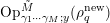 $\text{Op}_{\unicode[STIX]{x1D6FE}_{1}\cdots \unicode[STIX]{x1D6FE}_{M};y}^{\tilde{M}}(\unicode[STIX]{x1D70C}_{q}^{\text{new}})$
. The reader can consult [Reference Magee, Oh and WinterMOW19, § 5.3] for more details. The proof of Proposition 5.6 will take up the remaining §§ 5.3, 5.4 of the present section.
Proof of Proposition 3.12 from Proposition 5.6.
Import all the constants from Proposition 5.6. Recall we are given
 $t_{0}$
such that we assume
 $s=\unicode[STIX]{x1D70E}+it$
with
 $|t|\leqslant t_{0}$
. We also assume
 $|\unicode[STIX]{x1D70E}|<\unicode[STIX]{x1D70E}_{1}$
. We choose
 $M=\lfloor c^{\prime }\log q\rfloor$
where
 $c^{\prime }>0$
is chosen such that
 $\unicode[STIX]{x1D6EC}^{-M}\ll q^{-D}$
. ThenFootnote
21
 $N\approx c_{0}\log q$
. Note that
 $$\begin{eqnarray}\displaystyle \Vert \unicode[STIX]{x1D70C}_{q}^{\text{new}}(\unicode[STIX]{x1D6E9}_{\unicode[STIX]{x1D6FE}_{M}}^{\ast })^{-1}\cdots \unicode[STIX]{x1D70C}(\unicode[STIX]{x1D6E9}_{\unicode[STIX]{x1D6FE}_{1}}^{\ast })^{-1}F(\unicode[STIX]{x1D6FC}_{\unicode[STIX]{x1D6FE}_{1}\cdots \unicode[STIX]{x1D6FE}_{M}}o)\Vert _{{\mathcal{W}}}\leqslant \Vert F\Vert _{C^{1}} & & \displaystyle \nonumber\end{eqnarray}$$
as
 $\unicode[STIX]{x1D70C}_{q}^{\text{new}}$
is unitary.
Lemma 5.5 and using the triangle inequality gives a constant
 $C>0$
such that for any
 $F\in C^{1}(\unicode[STIX]{x1D6EF};\unicode[STIX]{x1D70C}_{q}^{\text{new}})$
 $$\begin{eqnarray}\displaystyle \Vert \mathbf{L}_{s,\unicode[STIX]{x1D70C}_{q}^{\text{new}}}^{N}F\Vert _{C^{1}}\leqslant Cq^{-D}\Vert F\Vert _{C^{1}}\mathop{\sum }_{\unicode[STIX]{x1D6FE}_{1},\ldots ,\unicode[STIX]{x1D6FE}_{M}}e^{R_{\unicode[STIX]{x1D70E}}^{(M)}(\unicode[STIX]{x1D6FC}_{\unicode[STIX]{x1D6FE}_{1}\cdots \unicode[STIX]{x1D6FE}_{M}}o)}=Cq^{-D}\Vert F\Vert _{C^{1}} & & \displaystyle \nonumber\end{eqnarray}$$
since the sum is
 $\mathbf{L}_{\unicode[STIX]{x1D70E}}^{M}[1]=1$
. Now by increasing
 $q_{0}$
if necessary, we ensure that when
 $q>q_{0}$
,
 $Cq^{-D}\leqslant q^{-D/2}$
.
Now given an arbitrary
 $N^{\prime }$
, we can write
 $N^{\prime }=aN+b$
with
 $0\leqslant b<N\approx c_{0}\log q$
. Since the operator norm of
 $\mathbf{L}_{s,\unicode[STIX]{x1D70C}_{q}^{\text{new}}}$
is bounded (by comparison to
 $\mathbf{L}_{\unicode[STIX]{x1D70E}}$
) by a constant
 $K$
depending on
 $t_{0}$
, we obtain for any
 $F\in C^{1}(\unicode[STIX]{x1D6EF};\unicode[STIX]{x1D70C}_{q}^{\text{new}})$
 $$\begin{eqnarray}\displaystyle \Vert \mathbf{L}_{s,\unicode[STIX]{x1D70C}_{q}^{\text{new}}}^{N^{\prime }}F\Vert _{C^{1}}\leqslant K^{b}q^{-aD/2}\Vert F\Vert _{C^{1}}\leqslant q^{\unicode[STIX]{x1D702}}(1-\unicode[STIX]{x1D716})^{N^{\prime }}\Vert F\Vert _{C^{1}} & & \displaystyle \nonumber\end{eqnarray}$$
for some
 $\unicode[STIX]{x1D716},\unicode[STIX]{x1D702}>0$
.
To deal with
 $\unicode[STIX]{x1D70C}_{q}$
in place of
 $\unicode[STIX]{x1D70C}_{q}^{\text{new}}$
, we consider the groups
 $\unicode[STIX]{x1D6E4}_{q}(q^{\prime })$
that are defined to be the kernels of reduction modulo
 $q^{\prime }$
on
 $\unicode[STIX]{x1D6E4}_{q}$
.
We decompose
 $\unicode[STIX]{x1D70C}_{q}$
as
 $\bigoplus _{1\neq q^{\prime }|q}\unicode[STIX]{x1D70C}_{q^{\prime }}^{q}$
where
 $\unicode[STIX]{x1D70C}_{q^{\prime }}^{q}$
is the subrepresentation of
 $\ell _{0}^{2}(\unicode[STIX]{x1D6E4}_{q})$
corresponding to functions invariant under
 $\unicode[STIX]{x1D6E4}_{q}(q^{\prime })$
but not invariant by any
 $\unicode[STIX]{x1D6E4}_{q}(q^{\prime \prime })$
with
 $q^{\prime \prime }|q^{\prime }$
,
 $q^{\prime \prime }\neq q^{\prime }$
. This gives a splitting
 $$\begin{eqnarray}\displaystyle C^{1}(\unicode[STIX]{x1D6EF};\unicode[STIX]{x1D70C}_{q})=\mathop{\bigoplus }_{1\neq q^{\prime }|q}C^{1}(\unicode[STIX]{x1D6EF};\unicode[STIX]{x1D70C}_{q^{\prime }}^{q}). & & \displaystyle\end{eqnarray}$$
The action of the transfer operator
 $\mathbf{L}_{s,\unicode[STIX]{x1D70C}_{q}}$
on
 $C^{1}(\unicode[STIX]{x1D6EF};\unicode[STIX]{x1D70C}_{q^{\prime }}^{q})$
is intertwined with the action of
 $\mathbf{L}_{s,\unicode[STIX]{x1D70C}_{q^{\prime }}^{\text{new}}}$
on
 $C^{1}(\unicode[STIX]{x1D6EF};\unicode[STIX]{x1D70C}_{q^{\prime }}^{\text{new}})$
. Thus if
 $f\in C^{1}(\unicode[STIX]{x1D6EF};\unicode[STIX]{x1D70C}_{q})$
we can decompose
 $f=\sum _{1\neq q^{\prime }|q}f_{q^{\prime }}$
according to (47).
This is the point in the paper where the modulus
 $Q_{0}$
of Theorem 1.4 comes into play. We now assume
 $Q_{0}$
is the product of primes less than or equal to
 ${\leqslant}q_{0}$
, where
 $q_{0}$
is the constant fixed during this proof. In particular, if
 $q$
is coprime to
 $Q_{0}$
, then any
 $q^{\prime }|q$
has no proper divisors
 ${\leqslant}q_{0}$
. Under this assumption,
 $f_{q^{\prime }}=0$
if
 $q^{\prime }\leqslant q_{0}$
.
Now we have
 $$\begin{eqnarray}\displaystyle \Vert \mathbf{L}_{s,\unicode[STIX]{x1D70C}_{q}}^{N^{\prime }}f\Vert _{C^{1}}\leqslant \mathop{\sum }_{q_{0}<q^{\prime }|q}\Vert \mathbf{L}_{s,\unicode[STIX]{x1D70C}_{q^{\prime }}}^{N^{\prime }}f_{q^{\prime }}\Vert \leqslant \mathop{\sum }_{q_{0}<q^{\prime }|q}q^{\unicode[STIX]{x1D702}}(1-\unicode[STIX]{x1D716})^{N^{\prime }}\Vert f_{q^{\prime }}\Vert _{C^{1}}, & & \displaystyle \nonumber\end{eqnarray}$$
where we used the bound we previously obtained for the operator norm of
 $\mathbf{L}_{s,\unicode[STIX]{x1D70C}_{q^{\prime }}^{\text{new}}}^{N^{\prime }}$
to bound
 $\Vert \mathbf{L}_{s,\unicode[STIX]{x1D70C}_{q^{\prime }}}^{N^{\prime }}f_{q^{\prime }}\Vert _{C^{1}}$
. Since
 $\Vert f_{q^{\prime }}\Vert _{C^{1}}\leqslant \Vert f\Vert _{C^{1}}$
for each
 $q^{\prime }$
, and
 $q$
has fewer than
 $q^{\unicode[STIX]{x1D701}}$
divisors for some
 $\unicode[STIX]{x1D701}>0$
and all
 $q$
, by increasing
 $\unicode[STIX]{x1D702}$
if necessary the above can be bounded by
 $$\begin{eqnarray}\displaystyle q^{\unicode[STIX]{x1D702}}(1-\unicode[STIX]{x1D716})^{N^{\prime }}\Vert f\Vert _{C^{1}}. & & \displaystyle \nonumber\end{eqnarray}$$
This proves Proposition 3.12 with
 $\mathbf{L}_{s,\unicode[STIX]{x1D70C}_{q}^{\text{new}}}$
in place of
 ${\mathcal{L}}_{s,\unicode[STIX]{x1D70C}_{q}^{\text{new}}}$
. To convert between estimates for the unnormalized and normalized transfer operators, note that
 ${\mathcal{L}}_{s,\unicode[STIX]{x1D70C}_{q}}^{N}=\unicode[STIX]{x1D706}_{\unicode[STIX]{x1D70E}}^{N}h_{\unicode[STIX]{x1D70E}}\mathbf{L}_{s,\unicode[STIX]{x1D70C}_{q}}^{N}h_{\unicode[STIX]{x1D70E}}^{-1}$
. Multiplication and division by
 $h_{\unicode[STIX]{x1D70E}}$
is a uniformly bounded operator in
 $|\unicode[STIX]{x1D70E}|<\unicode[STIX]{x1D70E}_{1}$
by Theorem 3.10. Moreover, by Theorem 3.10 we can choose
 $\unicode[STIX]{x1D70E}_{1}^{\prime }<\unicode[STIX]{x1D70E}_{1}$
such that
 $\unicode[STIX]{x1D706}_{\unicode[STIX]{x1D70E}}<(1-\unicode[STIX]{x1D716})^{1/2}$
for all
 $|\unicode[STIX]{x1D70E}|<\unicode[STIX]{x1D70E}_{1}^{\prime }$
. Therefore under these assumptions on
 $\unicode[STIX]{x1D70E}$
we have for some
 $C>0$
, for all
 $N^{\prime }\geqslant 1$
,
 $$\begin{eqnarray}\displaystyle \Vert {\mathcal{L}}_{s,\unicode[STIX]{x1D70C}_{q}}^{N^{\prime }}f\Vert _{C^{1}}\leqslant Cq^{\unicode[STIX]{x1D702}}(1-\unicode[STIX]{x1D716})^{N^{\prime }/2} & & \displaystyle \nonumber\end{eqnarray}$$
which concludes the proof. ◻
5.3 Bounding the operator norm of convolution operators
Let
 $\unicode[STIX]{x1D70B}_{q}:\operatorname{Sp}(\mathbf{Z}^{2g},\unicode[STIX]{x1D714}_{\unicode[STIX]{x1D70B}})\rightarrow \unicode[STIX]{x1D6E4}_{q}$
be the reduction mod
 $q$
map. To improve the readability of the following argument we will write for
 $\unicode[STIX]{x1D6FE}_{0}$
-adapted
 $\unicode[STIX]{x1D6FE}$
 $$\begin{eqnarray}\displaystyle h_{\unicode[STIX]{x1D6FE}}:=\unicode[STIX]{x1D70B}_{q}(\unicode[STIX]{x1D6E9}_{\unicode[STIX]{x1D6FE}}^{\ast })^{-1}\in \unicode[STIX]{x1D6E4}_{q}. & & \displaystyle \nonumber\end{eqnarray}$$
Recall
 $N=M+\tilde{M}$
,
 $s=\unicode[STIX]{x1D70E}+it$
, and
 $o$
is an arbitrary but fixed point in
 $\unicode[STIX]{x1D6EF}$
. We are tasked with estimating the operator norm of the group algebra element
 $$\begin{eqnarray}\displaystyle \unicode[STIX]{x1D707}_{\unicode[STIX]{x1D6FE}_{1}\cdots \unicode[STIX]{x1D6FE}_{M};y}^{\tilde{M}}:=\mathop{\sum }_{\unicode[STIX]{x1D6FE}_{M+1},\ldots ,\unicode[STIX]{x1D6FE}_{N}}e^{R_{s}^{(N)}(\unicode[STIX]{x1D6FC}_{\unicode[STIX]{x1D6FE}_{1}\cdots \unicode[STIX]{x1D6FE}_{N}}y)}h_{\unicode[STIX]{x1D6FE}_{N}}h_{\unicode[STIX]{x1D6FE}_{N-1}}\cdots h_{\unicode[STIX]{x1D6FE}_{M+1}}\in \mathbf{C}[\unicode[STIX]{x1D6E4}_{q}] & & \displaystyle \nonumber\end{eqnarray}$$
as it acts by convolution on
 $\ell _{\text{new}}^{2}(\unicode[STIX]{x1D6E4}_{q})$
. Indeed, this is precisely the operator
 $\text{Op}_{\unicode[STIX]{x1D6FE}_{1}\cdots \unicode[STIX]{x1D6FE}_{M};y}^{\tilde{M}}(\unicode[STIX]{x1D70C}_{q}^{\text{new}})$
when restricted to
 $\ell _{\text{new}}^{2}(\unicode[STIX]{x1D6E4}_{q})$
. We view elements of
 $\mathbf{C}[\unicode[STIX]{x1D6E4}_{q}]$
interchangeably as complex-valued measures on
 $\unicode[STIX]{x1D6E4}_{q}$
. We write
 $\ast$
for the convolution of measures, this corresponds to multiplication in
 $\mathbf{C}[\unicode[STIX]{x1D6E4}_{q}]$
. Given
 $\unicode[STIX]{x1D707}\in \mathbf{C}[\unicode[STIX]{x1D6E4}_{q}]$
we write
 $|\unicode[STIX]{x1D707}|$
for the non-negative real measure obtained by taking absolute values of coefficients. We let
 $\tilde{\unicode[STIX]{x1D707}}$
be the measure defined by
 $\tilde{\unicode[STIX]{x1D707}}(g):=\overline{\unicode[STIX]{x1D707}(g^{-1})}$
. If
 $\unicode[STIX]{x1D707}_{1},\unicode[STIX]{x1D707}_{2}\in \mathbf{R}[\unicode[STIX]{x1D6E4}_{q}]$
we write
 $\unicode[STIX]{x1D707}_{1}\leqslant \unicode[STIX]{x1D707}_{2}$
if
 $\unicode[STIX]{x1D707}_{1}(g)\leqslant \unicode[STIX]{x1D707}_{2}(g)$
for all
 $g\in \unicode[STIX]{x1D6E4}_{q}$
.
Lemma 5.7. We have
 $$\begin{eqnarray}\displaystyle |\unicode[STIX]{x1D707}_{\unicode[STIX]{x1D6FE}_{1}\cdots \unicode[STIX]{x1D6FE}_{M};y}^{\tilde{M}}|\leqslant Ce^{R_{\unicode[STIX]{x1D70E}}^{(M)}(\unicode[STIX]{x1D6FC}_{\unicode[STIX]{x1D6FE}_{1}\cdots \unicode[STIX]{x1D6FE}_{M}}o)}\unicode[STIX]{x1D707}_{1} & & \displaystyle\end{eqnarray}$$
where
 $C>0$
is a constant and
 $$\begin{eqnarray}\displaystyle \unicode[STIX]{x1D707}_{1}=\mathop{\sum }_{\unicode[STIX]{x1D6FE}_{M+1},\ldots ,\unicode[STIX]{x1D6FE}_{N}}e^{R_{\unicode[STIX]{x1D70E}}^{(\tilde{M})}(\unicode[STIX]{x1D6FC}_{\unicode[STIX]{x1D6FE}_{M+1}\cdots \unicode[STIX]{x1D6FE}_{N}}o)}h_{\unicode[STIX]{x1D6FE}_{N}}h_{\unicode[STIX]{x1D6FE}_{N-1}}\cdots h_{\unicode[STIX]{x1D6FE}_{M+1}}. & & \displaystyle\end{eqnarray}$$
Proof. The proof is the same as [Reference Magee, Oh and WinterMOW19, Lemma A.2]. ◻
Note that although
 $\unicode[STIX]{x1D707}_{1}$
depends on
 $M,\tilde{M}$
, we suppress this dependence from now on. We now organize the ingredients for the proof of Proposition 5.6.
Proposition 5.8 (Majorization of
$\unicode[STIX]{x1D707}_{1}$
).

There is a constant
 $\unicode[STIX]{x1D716}>0$
such that for any
 $B>1$
, there exists an integer
 $L>0$
such that for all
 $K>0$
, if
 $\tilde{M}=LK$
, there is a measure
 $\unicode[STIX]{x1D707}_{2}$
such that
 $$\begin{eqnarray}\displaystyle \unicode[STIX]{x1D707}_{1}\leqslant \unicode[STIX]{x1D707}_{2}, & & \displaystyle\end{eqnarray}$$
for all
 $\unicode[STIX]{x1D719}\in \ell _{0}^{2}(\unicode[STIX]{x1D6E4}_{q})$
,
 $$\begin{eqnarray}\displaystyle \Vert \unicode[STIX]{x1D707}_{2}\ast \unicode[STIX]{x1D719}\Vert _{\ell ^{2}}\leqslant (1-\unicode[STIX]{x1D716})^{K}\Vert \unicode[STIX]{x1D707}_{2}\Vert _{1}\Vert \unicode[STIX]{x1D719}\Vert _{\ell ^{2}}, & & \displaystyle\end{eqnarray}$$
and
 $$\begin{eqnarray}\displaystyle \Vert \unicode[STIX]{x1D707}_{2}\Vert _{1}\leqslant B^{K}\Vert \unicode[STIX]{x1D707}_{1}\Vert _{1}. & & \displaystyle\end{eqnarray}$$
The proof of this proposition is deferred to the next section. Note that we would like to have (51) for
 $\unicode[STIX]{x1D707}_{1}$
, or even better, the analogous result for
 $\unicode[STIX]{x1D707}_{\unicode[STIX]{x1D6FE}_{1}\cdots \unicode[STIX]{x1D6FE}_{M};y}^{\tilde{M}}$
. However, we only know
 $|\unicode[STIX]{x1D707}_{\unicode[STIX]{x1D6FE}_{1}\cdots \unicode[STIX]{x1D6FE}_{M};y}^{\tilde{M}}|\ll e^{R_{\unicode[STIX]{x1D70E}}^{(M)}(\unicode[STIX]{x1D6FC}_{\unicode[STIX]{x1D6FE}_{1}\cdots \unicode[STIX]{x1D6FE}_{M}}o)}\unicode[STIX]{x1D707}_{2}$
from which it is not obvious how to convert (51) into Proposition 5.8.
The solution is to first use Proposition 5.8 to deduce that the
 $\ell ^{2}$
norm of
 $\widetilde{\unicode[STIX]{x1D707}_{2}}\ast \unicode[STIX]{x1D707}_{2}$
is small, and hence the
 $\ell ^{2}$
norm of
 $\widetilde{\unicode[STIX]{x1D707}_{\unicode[STIX]{x1D6FE}_{1}\cdots \unicode[STIX]{x1D6FE}_{M};y}^{\tilde{M}}}\ast \unicode[STIX]{x1D707}_{\unicode[STIX]{x1D6FE}_{1}\cdots \unicode[STIX]{x1D6FE}_{M};y}^{\tilde{M}}$
is small. This will be done using the following lemma.
Lemma 5.9 [Reference Magee, Oh and WinterMOW19, Proposition A.8].
For any measure
 $\unicode[STIX]{x1D708}$
on
 $\unicode[STIX]{x1D6E4}_{q}$
, we have
 $$\begin{eqnarray}\displaystyle \Vert \tilde{\unicode[STIX]{x1D708}}\ast \unicode[STIX]{x1D708}\Vert _{2}\leqslant \frac{\Vert \unicode[STIX]{x1D708}\Vert _{1}^{2}}{|\unicode[STIX]{x1D6E4}_{q}|^{1/2}}+\Vert \unicode[STIX]{x1D708}\Vert _{1}\Vert \unicode[STIX]{x1D708}\Vert _{\ell _{0}^{2}(\unicode[STIX]{x1D6E4}_{q})}. & & \displaystyle \nonumber\end{eqnarray}$$
Here
 $\Vert \unicode[STIX]{x1D708}\Vert _{\ell _{0}^{2}(\unicode[STIX]{x1D6E4}_{q})}$
is the operator norm of
 $\unicode[STIX]{x1D708}$
acting by convolution on
 $\ell _{0}^{2}(\unicode[STIX]{x1D6E4}_{q})$
.
Proof. This is proved in [Reference Magee, Oh and WinterMOW19, proof of Proposition A.8]. ◻
In the previous lemma, we will take
 $\unicode[STIX]{x1D708}=\unicode[STIX]{x1D707}_{2}$
. When we succeed in proving
 $\Vert \widetilde{\unicode[STIX]{x1D707}_{\unicode[STIX]{x1D6FE}_{1}\cdots \unicode[STIX]{x1D6FE}_{M};y}^{\tilde{M}}}\ast \unicode[STIX]{x1D707}_{\unicode[STIX]{x1D6FE}_{1}\cdots \unicode[STIX]{x1D6FE}_{M};y}^{\tilde{M}}\Vert _{2}$
is small, we will then need a way to convert this into information on the operator norm of
 $\unicode[STIX]{x1D707}_{\unicode[STIX]{x1D6FE}_{1}\cdots \unicode[STIX]{x1D6FE}_{M};y}$
. It is here that the quasirandomness property of
 $\operatorname{Sp}_{2g}(\mathbf{Z}/q\mathbf{Z})$
is crucially used.
Lemma 5.10. For some absolute
 $C,D>0$
 $$\begin{eqnarray}\displaystyle \Vert \unicode[STIX]{x1D707}_{\unicode[STIX]{x1D6FE}_{1}\cdots \unicode[STIX]{x1D6FE}_{M};y}^{\tilde{M}}\Vert _{\ell _{\text{new}}^{2}(\unicode[STIX]{x1D6E4}_{q})}\leqslant C\biggl(\frac{|\unicode[STIX]{x1D6E4}_{q}|\Vert \widetilde{\unicode[STIX]{x1D707}_{\unicode[STIX]{x1D6FE}_{1}\cdots \unicode[STIX]{x1D6FE}_{M};y}^{\tilde{M}}}\ast \unicode[STIX]{x1D707}_{\unicode[STIX]{x1D6FE}_{1}\cdots \unicode[STIX]{x1D6FE}_{M};y}^{\tilde{M}}\Vert _{2}^{2}}{q^{D}}\biggr)^{1/4}. & & \displaystyle \nonumber\end{eqnarray}$$
Here
 $\Vert .\Vert _{2}^{2}$
denotes the
 $\ell ^{2}$
norm of the measure on
 $\unicode[STIX]{x1D6E4}_{q}$
and
 $\Vert \unicode[STIX]{x1D707}_{\unicode[STIX]{x1D6FE}_{1}\cdots \unicode[STIX]{x1D6FE}_{M};y}^{\tilde{M}}\Vert _{\ell _{\text{new}}^{2}(\unicode[STIX]{x1D6E4}_{q})}$
is the operator norm of
 $\unicode[STIX]{x1D707}_{\unicode[STIX]{x1D6FE}_{1}\cdots \unicode[STIX]{x1D6FE}_{M};y}^{\tilde{M}}$
acting on the new subspace of
 $\ell ^{2}(\unicode[STIX]{x1D6E4}_{q})$
.
Proof. We need to use the lower bound for the degree of new irreducible representations of
 $\operatorname{Sp}((\mathbf{Z}/q\mathbf{Z})^{2g},\unicode[STIX]{x1D714}_{\unicode[STIX]{x1D70B}})$
that is given in Proposition 6.1. Supposing that the smallest new irreducible representation has
 $\gg q^{D}$
, then by the trace formula argument of [Reference Magee, Oh and WinterMOW19, Lemma A.7] the largest eigenvalue of
 $A^{\ast }A$
where
 $A:=\unicode[STIX]{x1D707}_{\unicode[STIX]{x1D6FE}_{1}\cdots \unicode[STIX]{x1D6FE}_{M};y}^{\tilde{M}}\ast$
acting on
 $\ell _{\text{new}}^{2}(\unicode[STIX]{x1D6E4}_{q})$
satisfies
 $$\begin{eqnarray}\displaystyle \unicode[STIX]{x1D706}^{2}q^{D}\leqslant C^{\prime }|\unicode[STIX]{x1D6E4}_{q}|\Vert \widetilde{\unicode[STIX]{x1D707}_{\unicode[STIX]{x1D6FE}_{1}\cdots \unicode[STIX]{x1D6FE}_{M};y}^{\tilde{M}}}\ast \unicode[STIX]{x1D707}_{\unicode[STIX]{x1D6FE}_{1}\cdots \unicode[STIX]{x1D6FE}_{M};y}^{\tilde{M}}\Vert _{2}^{2}. & & \displaystyle \nonumber\end{eqnarray}$$
The crucial point is that the eigenvalue appears with high multiplicity in the trace formula, an idea that goes back to Sarnak and Xue [Reference Sarnak and XueSX91]. Since
 $\Vert A\Vert =\unicode[STIX]{x1D706}^{1/2}$
the lemma follows.◻
Now we can prove Proposition 5.6, modulo the deferred proof of Proposition 5.8.
Proof of Proposition 5.6.
We now make precise the argument we outlined before. Let
 $\unicode[STIX]{x1D716}>0$
be the constant from Proposition 5.8. Choose
 $B>1$
such that for all
 $q\geqslant 2$
,
 $$\begin{eqnarray}\displaystyle \log B\leqslant -\text{log}(1-\unicode[STIX]{x1D716})\frac{D}{2}\frac{\log q}{\log |\unicode[STIX]{x1D6E4}_{q}|}, & & \displaystyle \nonumber\end{eqnarray}$$
where
 $D$
is the constant from Lemma 5.10. The reason for this choice will be pointed out shortly. Apply Proposition 5.8 for this
 $B$
to obtain a constant
 $L$
and measure
 $\unicode[STIX]{x1D707}_{2}$
such that
 $\unicode[STIX]{x1D707}_{1}\leqslant \unicode[STIX]{x1D707}_{2}$
. We let
 $\tilde{M}=LK$
as in Proposition 5.8. Combining Proposition 5.8 and Lemma 5.9 we obtain
 $$\begin{eqnarray}\displaystyle \Vert \widetilde{\unicode[STIX]{x1D707}_{2}}\ast \unicode[STIX]{x1D707}_{2}\Vert _{2}\leqslant \Vert \unicode[STIX]{x1D707}_{2}\Vert _{1}^{2}\biggl(\frac{1}{|\unicode[STIX]{x1D6E4}_{q}|^{1/2}}+(1-\unicode[STIX]{x1D716})^{K}\biggr)\leqslant B^{2K}\Vert \unicode[STIX]{x1D707}_{1}\Vert _{1}^{2}\biggl(\frac{1}{|\unicode[STIX]{x1D6E4}_{q}|^{1/2}}+(1-\unicode[STIX]{x1D716})^{K}\biggr). & & \displaystyle \nonumber\end{eqnarray}$$
We can evaluate
 $\Vert \unicode[STIX]{x1D707}_{1}\Vert _{1}$
by
 $$\begin{eqnarray}\displaystyle \Vert \unicode[STIX]{x1D707}_{1}\Vert _{1}=\mathop{\sum }_{\unicode[STIX]{x1D6FE}_{M+1},\ldots ,\unicode[STIX]{x1D6FE}_{N}}e^{R_{\unicode[STIX]{x1D70E}}^{(\tilde{M})}(\unicode[STIX]{x1D6FC}_{\unicode[STIX]{x1D6FE}_{M+1}\cdots \unicode[STIX]{x1D6FE}_{N}}o)}=\mathbf{L}_{\unicode[STIX]{x1D70E}}^{\tilde{M}}[1](o)=1. & & \displaystyle \nonumber\end{eqnarray}$$
Hence
 $$\begin{eqnarray}\displaystyle \Vert \widetilde{\unicode[STIX]{x1D707}_{2}}\ast \unicode[STIX]{x1D707}_{2}\Vert _{2}\leqslant B^{2K}\biggl(\frac{1}{|\unicode[STIX]{x1D6E4}_{q}|^{1/2}}+(1-\unicode[STIX]{x1D716})^{K}\biggr). & & \displaystyle \nonumber\end{eqnarray}$$
From (48) and
 $\unicode[STIX]{x1D707}_{1}\leqslant \unicode[STIX]{x1D707}_{2}$
we obtain
 $$\begin{eqnarray}\displaystyle \Vert \widetilde{\unicode[STIX]{x1D707}_{\unicode[STIX]{x1D6FE}_{1}\cdots \unicode[STIX]{x1D6FE}_{M};y}^{\tilde{M}}}\ast \unicode[STIX]{x1D707}_{\unicode[STIX]{x1D6FE}_{1}\cdots \unicode[STIX]{x1D6FE}_{M};y}^{\tilde{M}}\Vert _{2}\leqslant C^{2}e^{2R_{\unicode[STIX]{x1D70E}}^{(M)}(\unicode[STIX]{x1D6FC}_{\unicode[STIX]{x1D6FE}_{1}\cdots \unicode[STIX]{x1D6FE}_{M}}o)}B^{2K}\biggl(\frac{1}{|\unicode[STIX]{x1D6E4}_{q}|^{1/2}}+(1-\unicode[STIX]{x1D716})^{K}\biggr). & & \displaystyle \nonumber\end{eqnarray}$$
Using this as input to Lemma 5.10 gives
 $$\begin{eqnarray}\displaystyle \Vert \unicode[STIX]{x1D707}_{\unicode[STIX]{x1D6FE}_{1}\cdots \unicode[STIX]{x1D6FE}_{M};y}^{\tilde{M}}\Vert _{\ell _{\text{new}}^{2}(\unicode[STIX]{x1D6E4}_{q})}^{2} & \ll & \displaystyle \frac{|\unicode[STIX]{x1D6E4}_{q}|^{1/2}}{q^{D/2}}\Vert \widetilde{\unicode[STIX]{x1D707}_{\unicode[STIX]{x1D6FE}_{1}\cdots \unicode[STIX]{x1D6FE}_{M};y}^{\tilde{M}}}\ast \unicode[STIX]{x1D707}_{\unicode[STIX]{x1D6FE}_{1}\cdots \unicode[STIX]{x1D6FE}_{M};y}^{\tilde{M}}\Vert _{2}\nonumber\\ \displaystyle & \ll & \displaystyle e^{2R_{\unicode[STIX]{x1D70E}}^{(M)}(\unicode[STIX]{x1D6FC}_{\unicode[STIX]{x1D6FE}_{1}\cdots \unicode[STIX]{x1D6FE}_{M}}o)}\frac{B^{2K}}{q^{D/2}}(1+|\unicode[STIX]{x1D6E4}_{q}|^{1/2}(1-\unicode[STIX]{x1D716})^{K}).\nonumber\end{eqnarray}$$
We now choose our constant
 $c>0$
such that for
 $K=\lfloor c\log q\rfloor$
,
 $1\ll |\unicode[STIX]{x1D6E4}_{q}|^{1/2}(1-\unicode[STIX]{x1D716})^{K}\ll 1$
. The choice of
 $B$
ensures that for this
 $K$
,
 $B^{2K}/q^{D/2}\ll q^{-D/4}$
. Hence
 $$\begin{eqnarray}\displaystyle \Vert \unicode[STIX]{x1D707}_{\unicode[STIX]{x1D6FE}_{1}\cdots \unicode[STIX]{x1D6FE}_{M};y}^{\tilde{M}}\Vert _{\ell _{\text{new}}^{2}(\unicode[STIX]{x1D6E4}_{q})}^{2}\ll q^{-D/4}e^{2R_{\unicode[STIX]{x1D70E}}^{(M)}(\unicode[STIX]{x1D6FC}_{\unicode[STIX]{x1D6FE}_{1}\cdots \unicode[STIX]{x1D6FE}_{M}}o)}. & & \displaystyle \nonumber\end{eqnarray}$$
This proves the first inequality of Proposition 5.6 (replacing
 $D/8$
by
 $D$
). As remarked before, the second inequality uses essentially the same argument.◻
5.4 Decoupling II: majorizing
$\unicode[STIX]{x1D707}_{1}$

In this section we prove Proposition 5.8 by adapting arguments from [Reference Magee, Oh and WinterMOW19, Appendix] to the infinite alphabet setting, using also a different spectral gap input from property (T) that relies on our preparation of the set
 $\unicode[STIX]{x1D6F6}$
and its relation to the Rauzy–Veech group
 $G_{\unicode[STIX]{x1D70B}}$
. The key idea in the proof is that while
 $\unicode[STIX]{x1D707}_{1}$
is not a convolution, it can be majorized by a carefully chosen sum of convolutions.
We further decompose
 $$\begin{eqnarray}\displaystyle \tilde{M}=LK, & & \displaystyle\end{eqnarray}$$
where
 $L$
is going to be chosen to be a large constant, and decompose
 $\{M+1,\ldots ,N\}$
into blocks of size either 1,
 $L-1$
or
 $L$
. Let
 $$\begin{eqnarray}\displaystyle I_{i,j}=[\unicode[STIX]{x1D6FE}_{i},\unicode[STIX]{x1D6FE}_{i+1},\ldots ,\unicode[STIX]{x1D6FE}_{j}] & & \displaystyle \nonumber\end{eqnarray}$$
denote the block of all
 $\unicode[STIX]{x1D6FE}_{i^{\prime }}$
with
 $i\leqslant i^{\prime }\leqslant j$
. Rewrite the summation in (49) as
 $$\begin{eqnarray}\displaystyle \unicode[STIX]{x1D707}_{1}\,=\,\mathop{\sum }_{\!I_{M+1,M+L-1},I_{M+L+1,M+2L-1},\ldots ,I_{N-L+1,N-1}}\mathop{\sum }_{\unicode[STIX]{x1D6FE}_{M+L},\unicode[STIX]{x1D6FE}_{M+2L},\ldots ,\unicode[STIX]{x1D6FE}_{N}}\!e^{R_{\unicode[STIX]{x1D70E}}^{(\tilde{M})}(\unicode[STIX]{x1D6FC}_{\unicode[STIX]{x1D6FE}_{M+1}\cdots \unicode[STIX]{x1D6FE}_{N}}o)}h_{\unicode[STIX]{x1D6FE}_{N}}h_{\unicode[STIX]{x1D6FE}_{N-1}}\cdots h_{\unicode[STIX]{x1D6FE}_{M+1}}. & & \displaystyle \nonumber\\ \displaystyle & & \displaystyle\end{eqnarray}$$
This reordering of summation is permitted since the sums are suitably absolutely convergent by Theorem 3.10 and the following discussion. Following [Reference Magee, Oh and WinterMOW19, (A.15)], using contraction properties of
 $\unicode[STIX]{x1D6FC}_{\unicode[STIX]{x1D6FE}_{i}}$
and the bound (42) for the derivative of
 $R_{\unicode[STIX]{x1D70E}}^{(\tilde{M})}$
, one has the bounds
 $$\begin{eqnarray}\displaystyle \exp (-c\unicode[STIX]{x1D6EC}^{-L})^{K-1}\unicode[STIX]{x1D6FD}_{1}\unicode[STIX]{x1D6FD}_{2}\cdots \unicode[STIX]{x1D6FD}_{K}\leqslant e^{R_{\unicode[STIX]{x1D70E}}^{(\tilde{M})}(\unicode[STIX]{x1D6FC}_{\unicode[STIX]{x1D6FE}_{M+1}\cdots \unicode[STIX]{x1D6FE}_{N}}o)}\leqslant \exp (c\unicode[STIX]{x1D6EC}^{-L})^{K-1}\unicode[STIX]{x1D6FD}_{1}\unicode[STIX]{x1D6FD}_{2}\cdots \unicode[STIX]{x1D6FD}_{K}, & & \displaystyle\end{eqnarray}$$
where
 $$\begin{eqnarray}\displaystyle \unicode[STIX]{x1D6FD}_{K}=e^{R_{\unicode[STIX]{x1D70E}}^{(L)}(\unicode[STIX]{x1D6FC}_{\unicode[STIX]{x1D6FE}_{N-L+1}\cdots \unicode[STIX]{x1D6FE}_{N}}o)},\quad \unicode[STIX]{x1D6FD}_{j}=e^{R_{\unicode[STIX]{x1D70E}}^{(L)}(\unicode[STIX]{x1D6FC}_{\unicode[STIX]{x1D6FE}_{M+(j-1)L+1}\cdots \unicode[STIX]{x1D6FE}_{M+(j+1)L-1}}o)},\quad 1\leqslant j\leqslant K-1 & & \displaystyle \nonumber\end{eqnarray}$$
and
 $c>0$
is a constant. Notice the important feature that each
 $\unicode[STIX]{x1D6FD}_{j}$
depends on only one of
 $\unicode[STIX]{x1D6FE}_{M+jL}$
. Inserting the second inequality of (55) into (54) gives
 $$\begin{eqnarray}\displaystyle \unicode[STIX]{x1D707}_{1}\leqslant \unicode[STIX]{x1D707}_{2}:=\exp (c\unicode[STIX]{x1D6EC}^{-L})^{K-1}\mathop{\sum }_{I_{M+1,M+L-1},I_{M+L+1,M+2L-1},\ldots ,I_{N-L+1,N-1}}\unicode[STIX]{x1D702}_{K}\ast \unicode[STIX]{x1D702}_{K-1}\ast \cdots \ast \unicode[STIX]{x1D702}_{1}, & & \displaystyle\end{eqnarray}$$
where the
 $\unicode[STIX]{x1D702}_{j}=\unicode[STIX]{x1D702}_{j}(I_{M+1,M+L-1},I_{M+L+1,M+2L-1},\ldots ,I_{N-L+1,N-1})$
are given by
 $$\begin{eqnarray}\displaystyle \unicode[STIX]{x1D702}_{K} & := & \displaystyle \mathop{\sum }_{\unicode[STIX]{x1D6FE}_{N}}\unicode[STIX]{x1D6FD}_{K}(\unicode[STIX]{x1D6FE}_{N-L},\ldots ,\unicode[STIX]{x1D6FE}_{N})h_{\unicode[STIX]{x1D6FE}_{N}}\cdots h_{\unicode[STIX]{x1D6FE}_{N-L+1}},\nonumber\\ \displaystyle \unicode[STIX]{x1D702}_{j} & := & \displaystyle \mathop{\sum }_{\unicode[STIX]{x1D6FE}_{M+jL}}\unicode[STIX]{x1D6FD}_{j}(\unicode[STIX]{x1D6FE}_{M+(j-1)L+1},\ldots ,\unicode[STIX]{x1D6FE}_{M+(j+1)L-1})h_{\unicode[STIX]{x1D6FE}_{M+jL}}\cdots h_{\unicode[STIX]{x1D6FE}_{M+(j-1)L+1}},\quad 1\leqslant j\leqslant K-1.\nonumber\end{eqnarray}$$
We point out for the readers’ convenience that we have now defined
 $\unicode[STIX]{x1D707}_{2}$
. This proves (50).
To prove (51) we now aim for bounds on the operator norms of the measures
 $\unicode[STIX]{x1D702}_{j}$
acting by convolution on
 $\ell _{0}^{2}(\unicode[STIX]{x1D6E4}_{q})$
. We write
 $\Vert \unicode[STIX]{x1D702}_{j}\Vert _{\text{op}}$
for this operator norm. Consider, taking for example
 $1\leqslant j\leqslant K-1$
,
 $$\begin{eqnarray}\displaystyle \unicode[STIX]{x1D702}_{j}\ast \tilde{\unicode[STIX]{x1D702}_{j}}=\mathop{\sum }_{\unicode[STIX]{x1D6FE}_{M+jL},\unicode[STIX]{x1D6FE}_{M+jL}^{\prime }}\unicode[STIX]{x1D6FD}_{j}(\ldots ,\unicode[STIX]{x1D6FE}_{M+jL},\ldots )\unicode[STIX]{x1D6FD}_{j}(\ldots ,\unicode[STIX]{x1D6FE}_{M+jL}^{\prime },\ldots )h_{\unicode[STIX]{x1D6FE}_{M+jL}}(h_{\unicode[STIX]{x1D6FE}_{M+jL}^{\prime }})^{-1}. & & \displaystyle\end{eqnarray}$$
Since
 $$\begin{eqnarray}\displaystyle \Vert \unicode[STIX]{x1D702}_{j}\Vert _{\text{op}}=\Vert \tilde{\unicode[STIX]{x1D702}}_{j}\Vert _{\text{op}}=\sup _{\unicode[STIX]{x1D719}\in \ell _{0}^{2}(\unicode[STIX]{x1D6E4}_{q}):\Vert \unicode[STIX]{x1D719}\Vert =1}\langle \unicode[STIX]{x1D702}_{j}\ast \tilde{\unicode[STIX]{x1D702}}_{j}\unicode[STIX]{x1D719},\unicode[STIX]{x1D719}\rangle ^{1/2} & & \displaystyle\end{eqnarray}$$
we turn to estimating the operator norm of
 $\unicode[STIX]{x1D702}_{j}\ast \tilde{\unicode[STIX]{x1D702}_{j}}$
on
 $\ell _{0}^{2}(\unicode[STIX]{x1D6E4}_{q})$
. We need to both:
(i) estimate the values of
$\unicode[STIX]{x1D6FD}_{j}$
; and(ii) discuss the group elements
$h_{\unicode[STIX]{x1D6FE}_{M+jL}}(h_{\unicode[STIX]{x1D6FE}_{M+jL}})^{-1}$
.


These are both points of departure from [Reference Magee, Oh and WinterMOW19, Appendix], so we give more details.
(1) Continuing with
 $1\leqslant j\leqslant K-1$
(the edge case
 $j=K$
is similar) we have
 $$\begin{eqnarray}\displaystyle \unicode[STIX]{x1D6FD}_{j}(\ldots ,\unicode[STIX]{x1D6FE}_{M+jL},\ldots ) & = & \displaystyle e^{R_{\unicode[STIX]{x1D70E}}^{(L)}(\unicode[STIX]{x1D6FC}_{\unicode[STIX]{x1D6FE}_{M+(j-1)L+1}\cdots \unicode[STIX]{x1D6FE}_{M+(j+1)L-1}}o)}\nonumber\\ \displaystyle & = & \displaystyle \exp \biggl(\mathop{\sum }_{i=0}^{L-2}R_{\unicode[STIX]{x1D70E}}(\unicode[STIX]{x1D6FC}_{\unicode[STIX]{x1D6FE}_{M+(j-1)L+1+i}\cdots \unicode[STIX]{x1D6FE}_{M+(j+1)L-1}}o)\biggr)\exp (R_{\unicode[STIX]{x1D70E}}(\unicode[STIX]{x1D6FC}_{\unicode[STIX]{x1D6FE}_{M+jL}\cdots \unicode[STIX]{x1D6FE}_{M+(j+1)L-1}}o))\nonumber\\ \displaystyle & = & \displaystyle \exp \biggl(\mathop{\sum }_{i=0}^{L-2}R_{\unicode[STIX]{x1D70E}}(\unicode[STIX]{x1D6FC}_{\unicode[STIX]{x1D6FE}_{M+(j-1)L+1+i}\cdots \unicode[STIX]{x1D6FE}_{M+jL-1}}o)+O(\unicode[STIX]{x1D6EC}^{-i})\biggr)\nonumber\\ \displaystyle & & \displaystyle \times \exp (R_{\unicode[STIX]{x1D70E}}(\unicode[STIX]{x1D6FC}_{\unicode[STIX]{x1D6FE}_{M+jL}\cdots \unicode[STIX]{x1D6FE}_{M+(j+1)L-1}}o))\nonumber\\ \displaystyle & \asymp & \displaystyle \unicode[STIX]{x1D705}(\unicode[STIX]{x1D6FE}_{M+(j-1)L+1+i},\ldots ,\unicode[STIX]{x1D6FE}_{M+jL-1})\exp (R_{\unicode[STIX]{x1D70E}}(\unicode[STIX]{x1D6FC}_{\unicode[STIX]{x1D6FE}_{M+jL}\cdots \unicode[STIX]{x1D6FE}_{M+(j+1)L-1}}o)),\end{eqnarray}$$
where
 $\asymp$
means bounded above and below by a constant independent of all
 $\unicode[STIX]{x1D6FE}_{i}$
and
 $L$
, and
 $$\begin{eqnarray}\displaystyle \unicode[STIX]{x1D705}(\unicode[STIX]{x1D6FE}_{M+(j-1)L+1+i},\ldots ,\unicode[STIX]{x1D6FE}_{M+jL-1}):=\exp (R_{\unicode[STIX]{x1D70E}}^{(L-1)}(\unicode[STIX]{x1D6FC}_{\unicode[STIX]{x1D6FE}_{M+(j-1)L+1+i}\cdots \unicode[STIX]{x1D6FE}_{M+jL-1}}o)). & & \displaystyle \nonumber\end{eqnarray}$$
Note the arguments of
 $\unicode[STIX]{x1D705}$
are fixed given
 $\unicode[STIX]{x1D702}_{j}$
. Also note that for fixed
 $\unicode[STIX]{x1D702}_{j}$
the values
 $$\begin{eqnarray}\displaystyle \unicode[STIX]{x1D6FC}_{\unicode[STIX]{x1D6FE}_{M+jL+1}\cdots \unicode[STIX]{x1D6FE}_{M+(j+1)L-1}}o & & \displaystyle \nonumber\end{eqnarray}$$
lie in the same cylinder of depth one. On the other hand, the derivative of
 $R_{\unicode[STIX]{x1D70E}}\circ \unicode[STIX]{x1D6FC}_{\unicode[STIX]{x1D6FE}_{M+jL}}$
is uniformly bounded by (42), so the values in the exponent of (59) fluctuate by at most
 $O(1)$
while
 $\unicode[STIX]{x1D6FC}_{\unicode[STIX]{x1D6FE}_{M+jL}}$
is fixed. Therefore
 $$\begin{eqnarray}\displaystyle \unicode[STIX]{x1D6FD}_{j}(\ldots ,\unicode[STIX]{x1D6FE}_{M+jL},\ldots )\asymp \unicode[STIX]{x1D705}(\unicode[STIX]{x1D6FE}_{M+(j-1)L+1+i},\ldots ,\unicode[STIX]{x1D6FE}_{M+jL-1})\exp (R_{\unicode[STIX]{x1D70E}}(\unicode[STIX]{x1D6FC}_{\unicode[STIX]{x1D6FE}_{M+jL}}o)). & & \displaystyle\end{eqnarray}$$
In light of this estimate and the discussion after Theorem 3.10 concerning convergence of infinite sums, we see that
 $\unicode[STIX]{x1D702}_{j}$
and
 $\unicode[STIX]{x1D702}_{j}\ast \tilde{\unicode[STIX]{x1D702}}_{j}$
have finite
 $\ell _{1}$
norms. This supports our earlier justification of reordering of summations.
(2) Recall
 $\unicode[STIX]{x1D6F6}$
from Lemma 5.1. We can write
 $$\begin{eqnarray}\displaystyle \unicode[STIX]{x1D702}_{j}\ast \tilde{\unicode[STIX]{x1D702}_{j}}=\unicode[STIX]{x1D708}+\tilde{\unicode[STIX]{x1D708}}, & & \displaystyle \nonumber\end{eqnarray}$$
where
 $\unicode[STIX]{x1D708}$
is the contribution to (57) from
 $\unicode[STIX]{x1D6FE}_{M+jL},\unicode[STIX]{x1D6FE}_{M+jL}^{\prime }\in \unicode[STIX]{x1D6FE}_{0}.\unicode[STIX]{x1D6F6}$
and
 $\tilde{\unicode[STIX]{x1D708}}$
are the remaining contributions. Then the support of
 $\unicode[STIX]{x1D708}$
is the reduction mod
 $q$
of the set
 $$\begin{eqnarray}\displaystyle \unicode[STIX]{x1D6F4}=\{\unicode[STIX]{x1D6E9}_{\unicode[STIX]{x1D6FE}}^{\ast }.(\unicode[STIX]{x1D6E9}_{\unicode[STIX]{x1D6FE}^{\prime }}^{\ast })^{-1}:\unicode[STIX]{x1D6FE},\unicode[STIX]{x1D6FE}^{\prime }\in \unicode[STIX]{x1D6FE}_{0}.\unicode[STIX]{x1D6F6}\}. & & \displaystyle \nonumber\end{eqnarray}$$
By Lemma 5.1, the set
 $\unicode[STIX]{x1D6F4}$
generates the conjugate of
 $G_{\unicode[STIX]{x1D70B}}$
by
 $\unicode[STIX]{x1D6E9}_{\unicode[STIX]{x1D6FE}_{0}}^{\ast }$
. Call this conjugate group
 $G_{\unicode[STIX]{x1D70B}}^{\prime }$
.
We now bring these arguments (1) and (2) together. Let
 $\unicode[STIX]{x1D708}=\unicode[STIX]{x1D702}_{j}\ast \tilde{\unicode[STIX]{x1D702}_{j}}$
. Note that the operator formed from convolution by
 $\unicode[STIX]{x1D708}$
on
 $\ell _{0}^{2}(\unicode[STIX]{x1D6E4}_{q})$
is self-adjoint and positive. Therefore the operator norm of
 $\Vert \unicode[STIX]{x1D708}\Vert$
acting by convolution on
 $\ell _{0}^{2}(\unicode[STIX]{x1D6E4}_{q})$
is
 $$\begin{eqnarray}\displaystyle \Vert \unicode[STIX]{x1D708}\Vert _{\text{op}}=\sup _{\unicode[STIX]{x1D719}\in \ell _{0}^{2}(\unicode[STIX]{x1D6E4}_{q}),\Vert \unicode[STIX]{x1D719}\Vert =1}\langle \unicode[STIX]{x1D708}\ast \unicode[STIX]{x1D719},\unicode[STIX]{x1D719}\rangle . & & \displaystyle\end{eqnarray}$$
We need to use the following property of the action of
 $G_{\unicode[STIX]{x1D70B}}^{\prime }$
on
 $\unicode[STIX]{x1D6E4}_{q}$
.
Lemma 5.11 (No almost invariant vectors).
There is some
 $\unicode[STIX]{x1D716}>0$
such that for all odd
 $q$
, for all
 $\unicode[STIX]{x1D719}\in \ell _{0}^{2}(\unicode[STIX]{x1D6E4}_{q})$
with
 $\Vert \unicode[STIX]{x1D719}\Vert _{\ell ^{2}}=1$
there is some
 $g\in \unicode[STIX]{x1D6F4}$
such that if
 $g_{q}:=g\hspace{0.6em}{\rm mod}\hspace{0.2em}q$
, then
 $$\begin{eqnarray}\displaystyle \Vert g_{q}\ast \unicode[STIX]{x1D719}-\unicode[STIX]{x1D719}\Vert _{\ell ^{2}}>\unicode[STIX]{x1D716}. & & \displaystyle \nonumber\end{eqnarray}$$
Proof. By Theorem 2.3, when
 $q$
is odd,
 $G_{\unicode[STIX]{x1D70B}}^{\prime }$
maps onto
 $\unicode[STIX]{x1D6E4}_{q}$
. Hence
 $\ell _{0}^{2}(\unicode[STIX]{x1D6E4}_{q})$
has no invariant vectors. The statement of the lemma is then a consequence of Kazhdan’s property
 $(T)$
for finite index subgroups of
 $\operatorname{Sp}(\mathbf{Z}^{2g},\unicode[STIX]{x1D714}_{\unicode[STIX]{x1D70B}})$
[Reference KaždanKaž67] applied to
 $G_{\unicode[STIX]{x1D70B}}^{\prime }$
.◻
Write
 $$\begin{eqnarray}\displaystyle \unicode[STIX]{x1D708}=\mathop{\sum }_{g_{q}\in \unicode[STIX]{x1D6E4}_{q}}\unicode[STIX]{x1D708}_{g_{q}}g_{q}. & & \displaystyle \nonumber\end{eqnarray}$$
Let
 $\unicode[STIX]{x1D716}$
,
 $g_{q}^{0}$
be the constant (respectively group element) provided by Lemma 5.11 on inputting
 $\unicode[STIX]{x1D719}$
with
 $\Vert \unicode[STIX]{x1D719}\Vert =1$
. Then it is straightforward to check that
 $|\Re (\langle g_{q}^{0}\ast \unicode[STIX]{x1D719},\unicode[STIX]{x1D719}\rangle )|<(1-\unicode[STIX]{x1D716}^{\prime })$
where
 $\unicode[STIX]{x1D716}^{\prime }=\unicode[STIX]{x1D716}^{2}/2$
. Returning to (61), using
 $\unicode[STIX]{x1D708}_{g_{q}}=\unicode[STIX]{x1D708}_{(g_{q})^{-1}}$
from (57) we get
 $$\begin{eqnarray}\displaystyle \langle \unicode[STIX]{x1D708}\ast \unicode[STIX]{x1D719},\unicode[STIX]{x1D719}\rangle & = & \displaystyle \mathop{\sum }_{g_{q}\in \unicode[STIX]{x1D6E4}_{q}}\unicode[STIX]{x1D708}_{g_{q}}\langle g_{q}\ast \unicode[STIX]{x1D719},\unicode[STIX]{x1D719}\rangle =\mathop{\sum }_{g_{q}\in \unicode[STIX]{x1D6E4}_{q}}\unicode[STIX]{x1D708}_{g_{q}}\Re \langle g_{q}\ast \unicode[STIX]{x1D719},\unicode[STIX]{x1D719}\rangle \nonumber\\ \displaystyle & = & \displaystyle \unicode[STIX]{x1D708}_{g_{q}^{0}}\Re \langle g_{q}^{0}\ast \unicode[STIX]{x1D719},\unicode[STIX]{x1D719}\rangle +\mathop{\sum }_{g_{q}\neq g_{q}^{0}}\unicode[STIX]{x1D708}_{g_{q}}\Re \langle g_{q}\ast \unicode[STIX]{x1D719},\unicode[STIX]{x1D719}\rangle \nonumber\\ \displaystyle & {\leqslant} & \displaystyle (1-\unicode[STIX]{x1D716}^{\prime })\unicode[STIX]{x1D708}_{g_{q}^{0}}+\mathop{\sum }_{g_{q}\neq g_{q}^{0}}\unicode[STIX]{x1D708}_{g_{q}}=\Vert \unicode[STIX]{x1D708}\Vert _{1}-\unicode[STIX]{x1D716}^{\prime }\unicode[STIX]{x1D708}_{g_{q}^{0}}.\nonumber\end{eqnarray}$$
Also, from (60), and that
 $\sum _{\unicode[STIX]{x1D6FE}_{M+jL}}\exp (R_{\unicode[STIX]{x1D70E}}(\unicode[STIX]{x1D6FC}_{\unicode[STIX]{x1D6FE}_{M+jL}}o))=\mathbf{L}_{\unicode[STIX]{x1D70E}}[1](o)=1$
, we get
 $$\begin{eqnarray}\displaystyle \unicode[STIX]{x1D708}_{g_{q}^{0}}\geqslant C\Vert \unicode[STIX]{x1D708}\Vert _{1} & & \displaystyle \nonumber\end{eqnarray}$$
with constant
 $C$
independent of
 $\unicode[STIX]{x1D708}_{g_{q}^{0}}$
and
 $\unicode[STIX]{x1D702}_{j}$
. So combining this with the preceding estimate and (61) we get
 $$\begin{eqnarray}\displaystyle \Vert \unicode[STIX]{x1D708}\Vert _{\text{op}}\leqslant \Vert \unicode[STIX]{x1D708}\Vert _{1}(1-\unicode[STIX]{x1D716}^{\prime \prime }) & & \displaystyle \nonumber\end{eqnarray}$$
for some
 $\unicode[STIX]{x1D716}^{\prime \prime }>0$
. Inserting this into (58) gives
 $$\begin{eqnarray}\displaystyle \Vert \unicode[STIX]{x1D702}_{j}\Vert _{\text{op}}\leqslant \Vert \unicode[STIX]{x1D702}_{j}\Vert _{\ell ^{1}}(1-\unicode[STIX]{x1D716}^{\prime \prime })^{1/2}. & & \displaystyle\end{eqnarray}$$
Using (62) in (56) gives for any
 $\unicode[STIX]{x1D719}\in \ell _{0}^{2}(\unicode[STIX]{x1D6E4}_{q})$
 $$\begin{eqnarray}\displaystyle \Vert \unicode[STIX]{x1D707}_{2}\ast \unicode[STIX]{x1D719}\Vert _{\ell ^{2}}\leqslant (1-\unicode[STIX]{x1D716}^{\prime \prime })^{K/2}\Vert \unicode[STIX]{x1D707}_{2}\Vert _{1}\Vert \unicode[STIX]{x1D719}\Vert _{\ell ^{2}}. & & \displaystyle \nonumber\end{eqnarray}$$
This proves (51). It remains to choose
 $L$
so that (52) holds. To do so, we estimate
 $\Vert \unicode[STIX]{x1D707}_{2}\Vert _{1}$
. We have
 $$\begin{eqnarray}\displaystyle \Vert \unicode[STIX]{x1D707}_{2}\Vert _{1}\leqslant \exp (c\unicode[STIX]{x1D6EC}^{-L})^{K-1}\mathop{\sum }_{I_{M+1,M+L-1},I_{M+L+1,M+2L-1},\ldots ,I_{N-L+1,N-1}}\mathop{\sum }_{\unicode[STIX]{x1D6FE}_{M+L},\unicode[STIX]{x1D6FE}_{M+2L},\ldots ,\unicode[STIX]{x1D6FE}_{N}}\unicode[STIX]{x1D6FD}_{1}\cdots \unicode[STIX]{x1D6FD}_{K}. & & \displaystyle \nonumber\end{eqnarray}$$
We now use the first inequality of (55) to get
 $$\begin{eqnarray}\displaystyle \Vert \unicode[STIX]{x1D707}_{2}\Vert _{1}\,\leqslant \,\exp (2c\unicode[STIX]{x1D6EC}^{^{-L}})^{K-1}\mathop{\sum }_{\!I_{M+1,M+L-1},I_{M+L+1,M+2L-1},\ldots ,I_{N-L+1,N-1}}\mathop{\sum }_{\unicode[STIX]{x1D6FE}_{M+L},\unicode[STIX]{x1D6FE}_{M+2L},\ldots ,\unicode[STIX]{x1D6FE}_{N}}\!e^{R_{\unicode[STIX]{x1D70E}}^{(\tilde{M})}(\unicode[STIX]{x1D6FC}_{\unicode[STIX]{x1D6FE}_{M+1}\cdots \unicode[STIX]{x1D6FE}_{N}}o)}. & & \displaystyle \nonumber\end{eqnarray}$$
But from inspection of (54), the above is
 $\exp (2c\unicode[STIX]{x1D6EC}^{^{-L}})^{K-1}\Vert \unicode[STIX]{x1D707}_{1}\Vert$
. Recall
 $B$
is the quantifier from Proposition 5.8. We now choose
 $L$
large enough so that
 $$\begin{eqnarray}\displaystyle \exp (2c\unicode[STIX]{x1D6EC}^{^{-L}})\leqslant B. & & \displaystyle \nonumber\end{eqnarray}$$
This gives
 $$\begin{eqnarray}\displaystyle \Vert \unicode[STIX]{x1D707}_{2}\Vert _{1}\leqslant \exp (2c\unicode[STIX]{x1D6EC}^{^{-L}})^{K-1}\Vert \unicode[STIX]{x1D707}_{1}\Vert \leqslant B^{K}\Vert \unicode[STIX]{x1D707}_{1}\Vert & & \displaystyle \nonumber\end{eqnarray}$$
and completes the proof of Proposition 5.8.
6 Quasirandomness
In this section we show that ‘new’ representations of
 $\operatorname{Sp}((\mathbf{Z}/q\mathbf{Z})^{2g},\unicode[STIX]{x1D714}_{{\mathcal{M}}})$
have large dimension. This is a version of the quasirandomness property of a group that takes into account the level structure of the family of groups
 $\operatorname{Sp}((\mathbf{Z}/q\mathbf{Z})^{2g},\unicode[STIX]{x1D714}_{{\mathcal{M}}})$
.
Proposition 6.1 (Quasirandomness estimates).
There is
 $C>0$
and
 $D>0$
such that any irreducible representation of
 $\operatorname{Sp}((\mathbf{Z}/q\mathbf{Z})^{2g},\unicode[STIX]{x1D714}_{{\mathcal{M}}})$
that does not factor through
 $$\begin{eqnarray}\displaystyle \operatorname{Sp}((\mathbf{Z}/q\mathbf{Z})^{2g},\unicode[STIX]{x1D714}_{{\mathcal{M}}})\rightarrow \operatorname{Sp}((\mathbf{Z}/q_{1}\mathbf{Z})^{2g},\unicode[STIX]{x1D714}_{{\mathcal{M}}}) & & \displaystyle \nonumber\end{eqnarray}$$
for some
 $q_{1}|q$
has dimension
 ${\geqslant}Cq^{D}$
.
We follow the type of argument given by Kelmer and Silberman in [Reference Kelmer and SilbermanKS13, § 4] for rank-one groups (see also [Reference MageeMag15] for a small improvement to that argument). We may treat the group
 $\operatorname{Sp}_{2g}(\mathbf{Z})$
without loss of generality, that is, we assume the symplectic form is the standard one. Let
 $g\geqslant 2$
. Let
 $q\in \mathbf{N}$
and let
 $(\unicode[STIX]{x1D70C},{\mathcal{W}})$
be an irreducible unitary representation of
 $\operatorname{Sp}_{2g}(\mathbf{Z}/q\mathbf{Z})$
that is not obtained by a composition
 $$\begin{eqnarray}\displaystyle \operatorname{Sp}_{2g}(\mathbf{Z}/q\mathbf{Z})\rightarrow \operatorname{Sp}_{2g}(\mathbf{Z}/q_{1}\mathbf{Z})\xrightarrow[{}]{\unicode[STIX]{x1D70C}^{\prime }}U({\mathcal{W}}) & & \displaystyle \nonumber\end{eqnarray}$$
with
 $q_{1}|q$
. We refer to this property as
 $\unicode[STIX]{x1D70C}$
being new.
6.1 The case when
$q$
is prime

For
 $p$
an odd prime, let
 $\mathbb{F}_{p}$
denote the finite field with
 $p$
elements. The table of Seitz and Zalesskii in [Reference Seitz and ZalesskiiSZ93, Table 1] implies that
 $P\operatorname{Sp}_{2g}(\mathbb{F}_{p})$
has no projective complex irreducible representation of dimension
 ${<}\frac{1}{2}(p^{g}-1)$
and hence this is also a lower bound for the dimension of an irreducible representation of
 $\operatorname{Sp}_{2g}(\mathbb{F}_{p})$
.
6.2 The case
$q=p^{r}$

In this section we prove the following.
Proposition 6.2. There is some
 $C>0$
depending only on
 $g$
such that for all
 $r\geqslant 2$
, letting
 $R:=\lfloor r/2\rfloor$
any new representation
 $(\unicode[STIX]{x1D70C},{\mathcal{W}})$
of
 $\operatorname{Sp}_{2g}(\mathbf{Z}/p^{r}\mathbf{Z})$
has dimension at least
 $$\begin{eqnarray}\displaystyle \dim \unicode[STIX]{x1D70C}\geqslant Cp^{R}. & & \displaystyle \nonumber\end{eqnarray}$$
Let
 $q=p^{r}$
. Write
 $H_{q}:=\operatorname{Sp}_{2g}(\mathbf{Z}/q\mathbf{Z})$
and for
 $q^{\prime }|q$
let
 $H_{q}(q^{\prime })$
be the kernel of the reduction modulo
 $q^{\prime }$
map
 $$\begin{eqnarray}\displaystyle H_{q}\rightarrow H_{q^{\prime }}. & & \displaystyle \nonumber\end{eqnarray}$$
Let
 $\mathfrak{g}(\mathbf{Z}/q\mathbf{Z})$
denote the Lie algebra of
 $\operatorname{Sp}_{2g}$
over
 $\mathbf{Z}/q\mathbf{Z}$
. We view this as an abelian group. Let
 $R=\lfloor r/2\rfloor$
. The congruence subgroup
 $H_{p^{r}}(p^{r-R})$
is an abelian normal subgroup of
 $H_{p^{r}}$
that is naturally isomorphic to
 $\mathfrak{g}(\mathbf{Z}/p^{R}\mathbf{Z})$
. The action of
 $H_{p^{r}}$
on
 $H_{p^{r}}(p^{r-R})$
by conjugation descends to an action of
 $H_{p^{R}}$
. After using the isomorphism
 $H_{p^{r}}(p^{r-R})\cong \mathfrak{g}(\mathbf{Z}/p^{R}\mathbf{Z})$
this conjugation action is identified with the Adjoint action of
 $H_{p^{R}}$
on
 $\mathfrak{g}(\mathbf{Z}/p^{R}\mathbf{Z})$
, i.e.
 $$\begin{eqnarray}\displaystyle \operatorname{Ad}(g)v=gvg^{-1},\quad g\in H_{p^{R}},\quad v\in \mathfrak{g}(\mathbf{Z}/p^{R}\mathbf{Z}). & & \displaystyle \nonumber\end{eqnarray}$$
Let
 $(\unicode[STIX]{x1D70C},{\mathcal{W}})$
be a unitary representation of
 $H_{q}$
. Suppose
 $R\geqslant 1$
. If
 $\unicode[STIX]{x1D70C}$
is trivial when restricted to
 $H_{q}(p^{R})$
, then
 $\unicode[STIX]{x1D70C}$
is not a new representation. More generally, if
 $\unicode[STIX]{x1D70C}$
is new, then the restriction of
 $\unicode[STIX]{x1D70C}$
to
 $H_{q}(p^{r-R})$
must not be trivial on any
 $H_{q}(p^{r-R+\unicode[STIX]{x1D702}})$
with
 $\unicode[STIX]{x1D702}\in \mathbf{Z}_{+}$
since these are also normal subgroups with
 $H_{q}/H_{q}(p^{r-R+\unicode[STIX]{x1D702}})\cong H_{p^{r-R+\unicode[STIX]{x1D702}}}$
. Notice
 $H_{q}(p^{r-R+\unicode[STIX]{x1D702}})\leqslant H_{q}(p^{r-R})$
corresponds to the inclusion
 $p^{\unicode[STIX]{x1D702}}\mathfrak{g}(\mathbf{Z}/p^{R-\unicode[STIX]{x1D702}}\mathbf{Z})\leqslant \mathfrak{g}(\mathbf{Z}/p^{R}\mathbf{Z})$
.
The strategy is to consider the
 $H_{p^{R}}$
invariant set of characters of
 $\mathfrak{g}(\mathbf{Z}/p^{R}\mathbf{Z})$
that appear when restricting
 $\unicode[STIX]{x1D70C}$
to
 $H_{p^{r}}(p^{r-R})\cong \mathfrak{g}(\mathbf{Z}/p^{R}\mathbf{Z})$
, since the size of this set gives a lower bound for the dimension of
 $\unicode[STIX]{x1D70C}$
.
The Killing form on
 $\mathfrak{g}(\mathbf{Z}/p^{R}\mathbf{Z})$
is non-degenerate which allows us to identify the unitary dual
 $\widehat{\mathfrak{g}(\mathbf{Z}/p^{R}\mathbf{Z})}$
with
 $\mathfrak{g}(\mathbf{Z}/p^{R}\mathbf{Z})$
. Under this identification, the co-Adjoint action on characters becomes an Adjoint action on
 $\mathfrak{g}(\mathbf{Z}/p^{R}\mathbf{Z})$
. Moreover any character that is non-trivial on each
 $H_{q}(p^{r-R+\unicode[STIX]{x1D702}})$
,
 $\unicode[STIX]{x1D702}\in \mathbf{Z}_{+}$
, becomes an element of
 $\mathfrak{g}(\mathbf{Z}/p^{R}\mathbf{Z})$
which is not congruent to
 $0$
modulo
 $p$
.
We have therefore reduced Proposition 6.2 to the following lemma.
Lemma 6.3. There is some
 $C>0$
depending only on
 $g$
such that for all
 $R\geqslant 1$
the
 $H_{p^{R}}$
-Adjoint orbit of any
 $X\in \mathfrak{g}(\mathbf{Z}/p^{R}\mathbf{Z})$
with
 $X\not \equiv 0\hspace{0.2em}{\rm mod}\hspace{0.2em}p$
has size
 $$\begin{eqnarray}\displaystyle |\operatorname{Ad}(H_{p^{R}}).X|\geqslant Cp^{R}. & & \displaystyle \nonumber\end{eqnarray}$$
Proof. By the orbit-stabilizer theorem the orbit has size at least
 $$\begin{eqnarray}\displaystyle \frac{|H_{p^{R}}|}{|C_{H_{p^{R}}}(X)|} & & \displaystyle\end{eqnarray}$$
where we write
 $C$
to stand for centralizer, and therefore
 $C_{H_{p^{r}}}(X)=\{h\in H_{p^{R}}:hXh^{-1}=X\}$
. Since
 $H_{p^{R}}$
is an
 $(R-1)$
-fold extension of
 $H_{p}$
by groups isomorphic to
 $\mathfrak{g}(\mathbb{F}_{p})$
we know
 $|H_{p^{R}}|=|H_{p}||\mathfrak{g}(\mathbb{F}_{p})|^{R-1}\gg p^{R.\dim (\operatorname{Sp}_{2g})}=p^{g(2g+1)R}$
. This gives the bound we will use for the numerator of (63).
Considering next the denominator of (63), by an elementary induction argument appearing in [Reference Kelmer and SilbermanKS13, Proof of Proposition 4.3]
 $$\begin{eqnarray}\displaystyle |C_{H_{p^{r}}}(X)|\leqslant |C_{H_{p}}(X\hspace{0.2em}{\rm mod}\hspace{0.2em}p)|\,|C_{\mathfrak{g}(\mathbb{F}_{p})}(X\hspace{0.2em}{\rm mod}\hspace{0.2em}p)|^{R-1}, & & \displaystyle\end{eqnarray}$$
where the latter centralizer is
 $C_{\mathfrak{g}(\mathbb{F}_{p})}(X\hspace{0.2em}{\rm mod}\hspace{0.2em}p)=\{y\in \mathfrak{g}(\mathbb{F}_{p}):[y,X\hspace{0.2em}{\rm mod}\hspace{0.2em}p]\equiv 0\}$
. According to Springer and Steinberg [Reference Springer and SteinbergSS70, II. 4.1, 4.2, IV. 2.26], the algebraic group
 $C_{\operatorname{Sp}_{2g}}(X\hspace{0.2em}{\rm mod}\hspace{0.2em}p)$
defined over
 $\mathbb{F}_{p}$
has a number of components bounded by a constant depending only on
 $g$
. By a bound of Nori [Reference NoriNor87, Lemma 3.5] each component can have at most
 $(p+1)^{\dim C_{\operatorname{Sp}_{2g}}(X\hspace{0.2em}{\rm mod}\hspace{0.2em}p)}$
points over
 $\mathbb{F}_{p}$
. But
 $\dim C_{\operatorname{Sp}_{2g}}(X\hspace{0.2em}{\rm mod}\hspace{0.2em}p)$
is also the dimension of the centralizer of
 $X\hspace{0.2em}{\rm mod}\hspace{0.2em}p$
in
 $\mathfrak{g}(\mathbb{F}_{p})$
, so we have now reduced the estimation of the right-hand side of (64) to a bound for
 $$\begin{eqnarray}\displaystyle \dim C_{\mathfrak{g}(\mathbb{F}_{p})}(X^{\prime }), & & \displaystyle \nonumber\end{eqnarray}$$
where
 $X^{\prime }=X\hspace{0.2em}{\rm mod}\hspace{0.2em}p$
is a non-zero element of
 $\mathfrak{g}(\mathbb{F}_{p})$
.
Assume the bound
 $\dim C_{\mathfrak{g}(\mathbb{F}_{p})}(X^{\prime })\leqslant \dim (\operatorname{Sp}_{2g})-e=g(2g+1)-e$
. Then putting our previous estimates together we obtain
 $$\begin{eqnarray}\displaystyle |\operatorname{Ad}(H_{p^{R}}).X|\gg \frac{p^{g(2g+1)R}}{(p+1)^{g(2g+1)-e}(p^{g(2g+1)-e})^{R-1}}\gg p^{eR}. & & \displaystyle \nonumber\end{eqnarray}$$
Since it is not particularly important here to optimize
 $e$
, we give the easy argument that one may take
 $e=1$
since
 $\mathfrak{g}(\mathbb{F}_{p})$
has no non-trivial center.Footnote
22
This gives the result stated in the lemma.◻
6.3 The case of general moduli
If
 $p_{i}$
are primes and
 $$\begin{eqnarray}\displaystyle q=\mathop{\prod }_{i=1}^{M}p_{i}^{m_{i}} & & \displaystyle \nonumber\end{eqnarray}$$
is the prime factorization of
 $q$
, then we have by the Chinese remainder theorem
 $$\begin{eqnarray}\displaystyle \operatorname{Sp}_{2g}(\mathbf{Z}/q\mathbf{Z})\cong \mathop{\prod }_{i=1}^{M}\operatorname{Sp}_{2g}(\mathbf{Z}/p_{i}^{m_{i}}\mathbf{Z}). & & \displaystyle \nonumber\end{eqnarray}$$
Then
 $\unicode[STIX]{x1D70C}$
splits as a tensor product
 $$\begin{eqnarray}\displaystyle \unicode[STIX]{x1D70C}=\mathop{\bigotimes }_{i=1}^{M}\unicode[STIX]{x1D70C}_{i}, & & \displaystyle \nonumber\end{eqnarray}$$
where
 $\unicode[STIX]{x1D70C}_{i}$
are irreducible representations of
 $\operatorname{Sp}_{2g}(\mathbf{Z}/p_{i}^{m_{i}}\mathbf{Z})$
. Since
 $\unicode[STIX]{x1D70C}$
is new, all of the
 $\unicode[STIX]{x1D70C}_{i}$
are new. Now using Proposition 6.2 and the bounds for the case of prime modulus from § 6.1 gives
 $$\begin{eqnarray}\displaystyle \dim \unicode[STIX]{x1D70C}\geqslant \mathop{\prod }_{i:m_{i}=1}\frac{1}{2}(p_{i}^{g}-1)\mathop{\prod }_{i:m_{i}>1}Cp_{i}^{\lfloor m_{i}/2\rfloor }\geqslant q^{1/2}(C^{\prime })^{-\unicode[STIX]{x1D714}(q)} & & \displaystyle \nonumber\end{eqnarray}$$
given
 $g\geqslant 2$
for some
 $C^{\prime }>1$
and
 $\unicode[STIX]{x1D714}(q)$
standing for the number of distinct prime factors of
 $q$
. But
 $(C^{\prime })^{\unicode[STIX]{x1D714}(q)}\,\ll _{\unicode[STIX]{x1D716}}\,q^{\unicode[STIX]{x1D716}}$
for any
 $\unicode[STIX]{x1D716}>0$
. This concludes the proof of Proposition 6.1; in fact, our proof shows that one may take
 $D$
as close as one likes to
 $1/2$
provided one chooses
 $C$
appropriately.
Acknowledgements
We thank Alex Eskin, Ilya Gekhtman, Sébastien Gouëzel, Rodolfo Gutiérrez-Romo, Carlos Matheus, Babak Modami, Hee Oh and Giulio Tiozzo for helpful discussions related to this work.









