2. Fundamental equations

Throughout this article we employ standard indicial notation together with the Einstein summation convention.

The basic equations for thermal convection in a Darcy porous medium with the Fourier law of heat conduction may be conveniently located in Straughan (Reference Straughan2008, p. 172–177) or in Straughan (Reference Straughan2015, p. 53–54). We now present these equations but we modify the governing equation involving the heat flux in order that it satisfies a heat flux law of Jeffreys type. The heat flux law of Jeffreys type is given in (2.2). Note that Fourier’s law follows from this by taking $\tau$ and $\zeta$ to be zero.

The nomenclature of a Jeffreys heat model is evidently due to Joseph & Preziosi (Reference Joseph and Preziosi1989), and as they correctly remark, Jeffreys work has nothing to do with heat transfer. Therefore, we clarify this. To describe a theory for viscoelastic flow of a fluid Jeffreys (Reference Jeffreys1929, p. 263–265) introduces an equation of form (in our notation)

(2.1) \begin{equation} \lambda \,\frac {\partial \sigma _{ij}}{\partial t}+\sigma _{ij}=2\mu d_{ij}+2\kappa \frac {\partial d_{ij}}{\partial t}, \end{equation}

where $\sigma _{ij}$ is the Cauchy extra stress tensor in a fluid, $d_{ij}$ is the symmetric part of the velocity gradient, $\mu$ is the dynamic viscosity of the fluid and $\lambda$ and $\kappa$ are positive coefficients. Jeffreys (Reference Jeffreys1929) refers to the left-hand side of (2.1) as an elastoviscous part, while Jeffreys (Reference Jeffreys1917) refers to the right-hand side of (2.1) as the firmoviscous part.

In this work we are interested in the analogue of (2.1) in heat conduction theory. Let $q_i$ denote the heat flux in a saturated porous medium and suppose $T$ is the temperature within that medium at the point $\boldsymbol {x}$ at time $t$ . The equation

(2.2) \begin{equation} \tau \frac {\partial q_i}{\partial t}+q_i=-k\frac {\partial T}{\partial x_i}-\zeta \frac {\partial ^2T}{\partial t\partial x_i}, \end{equation}

for $\tau ,k,\zeta$ positive constants, defines a Jeffreys heat theory, as observed by Giorgi et al. (Reference Giorgi, Morro and Zullo2024, equation 18), Giorgi & Zullo (Reference Giorgi and Zullo2026, equation 37). The equations for thermal convection in a saturated Darcy porous material may then be written

(2.3) \begin{align} v_i=-\frac {K}{\mu }\,\frac {\partial p}{\partial x_i}+\frac {\rho g{\hat \alpha } K}{\mu }\,T k_i, \end{align}

(2.4) \begin{align} \frac {\partial v_i}{\partial x_i}=0, \end{align}

(2.5) \begin{align} \rho c_{\!p}\, \left(\frac {\partial T}{\partial t}+v_i\frac {\partial T}{\partial x_i} \right)=-{\frac {\partial q_i}{\partial x_i}}, \end{align}

(2.6) \begin{align} \tau \frac {\partial q_i}{\partial t}+q_i=-k\frac {\partial T}{\partial x_i}-\zeta \frac {\partial ^2T}{\partial t\partial x_i}. \end{align}

In the above equations $x_i$ and $t$ denote space and time, $v_i,p,T$ and $q_i$ denote the fluid (pore-averaged) velocity, fluid pressure, temperature and heat flux, respectively. The terms $K,\mu ,g,{\hat \alpha },$ $\rho ,c_{\!p},k,\tau$ and $\zeta$ denote permeability, dynamic viscosity of the fluid, gravity, thermal expansion coefficient of the fluid, density of the fluid, specific heat at constant pressure, thermal conductivity, the Maxwell relaxation time and the relaxation time corresponding to the firmoviscous coefficient. The term $k_i$ refers to the vector $\boldsymbol {k}=(0,0,1)$ . Equation (2.3) represents Darcy’s law, (2.4) is conservation of mass, (2.5) is the energy balance equation and (2.6) is the Jeffreys heat evolution law.

Our goal is to analyse thermal convection in a horizontal layer of porous material governed by (2.3)–(2.6), and so we assume these equations hold in the domain $\mathbb{R}^2\times \{z\in (0,d)\}$ with gravity acting in the negative- $z$ direction. The boundary conditions we consider are

(2.7) \begin{equation} \begin{aligned} &w=v_3=0,\quad \textrm {on} \quad z=0,d,\\ &T=T_L,\quad \textrm {on} \quad z=0,\quad \quad &T=T_U,\quad \textrm {on} \quad z=d, \end{aligned} \end{equation}

with $T_L,T_U$ being constants such that $T_L\gt T_U$ .

The steady conduction solution whose stability we investigate is

(2.8) \begin{equation} {\bar {\boldsymbol {v}}}=(0,0,0),\quad {\bar T}=-\beta z+T_L,\quad {\bar {\boldsymbol {q}}}=(0,0,k\beta ), \end{equation}

where the temperature gradient has form

(2.9) \begin{equation} \beta =\frac {T_L-T_U}{d}. \end{equation}

3. Stability analysis

To analyse stability of (2.8) we introduce perturbations $(u_i,\pi ,\theta ,q_i)$ to the steady solution $({\bar v}_i,{\bar p},{\bar T},{\bar q}_i)$ and we derive the perturbation equations from (2.3)–(2.6). We introduce the non-dimensional variables by using the length, time, velocity, pressure, temperature and heat scales $L,{\mathcal T},U,P,T^{\sharp }$ and $Q$ given by

(3.1) \begin{equation} L=d,\quad {\mathcal T}=\frac {d^2}{\kappa },\quad U=\frac {\kappa }{d},\quad P=\frac {U\mu d}{K},\quad T^{\sharp }=U\sqrt {\frac {\beta d^2\nu }{\kappa g{\hat \alpha } K}},\quad Q=\frac {kT^{\sharp }}{d}. \end{equation}

Additionally, $\kappa ,\nu$ are the thermal diffusivity and kinematic viscosity given by $\kappa =k/(\rho c_{\!p})$ and $\nu =\mu /\rho$ . We define the Rayleigh number $Ra=R^2$ , and the non-dimensional Maxwell and Jeffreys coefficients $\lambda$ and $\mathfrak{J}$ , by

(3.2) \begin{equation} Ra=R^2=\frac {\beta d^2Kg{\hat \alpha }}{\nu \kappa }=\frac {(T_L-T_U){\rm d}Kg{\hat \alpha }}{\nu \kappa },\quad \lambda =\frac {\tau }{{\mathcal T}},\quad \mathfrak{J}=\frac {\zeta }{k{\mathcal T}}. \end{equation}

The non-dimensional system of nonlinear perturbation equations may then be shown to be

(3.3) \begin{align} &u_i=-\frac {\partial \pi }{\partial x_i}+R\theta k_i, \\[-12pt]\nonumber \end{align}

(3.4) \begin{align} &\frac {\partial u_i}{\partial x_i}=0, \\[-12pt]\nonumber \end{align}

(3.5) \begin{align} &\frac {\partial \theta }{\partial t}+u_i\frac {\partial \theta }{\partial x_i}=Rw-q_{i,i}, \\[-12pt]\nonumber \end{align}

(3.6) \begin{align} &\lambda \frac {\partial q_i}{\partial t}+q_i=-\frac {\partial \theta }{\partial x_i}-\mathfrak{J}\frac {\partial ^2\theta }{\partial t\partial x_i}, \end{align}

where $w$ now denotes $u_3$ .

Equations (3.3)–(3.6) hold on the domain $\mathbb{R}^2\times \{z\in (0,1)\}\times \{t\gt 0\}$ . The perturbation boundary conditions are

(3.7) \begin{equation} w=0,\quad \theta =0,\quad \textrm {on} \quad z=0,1, \end{equation}

together with the requirement that $(u_i,\pi ,\theta ,q_i)$ satisfy a plane tiling periodicity in the $(x,y)$ -plane.

To analyse the linear instability problem for (3.3)–(3.7) one linearises and then removes the pressure perturbation by taking the curl twice of (3.3). The representation $u_i=e^{\sigma t}u_i(\boldsymbol {x})$ is then used together with a similar one for $\theta$ and $q_i$ . This leads one to the system of equations

(3.8) \begin{equation} \begin{aligned} &-\Delta w+R\Delta ^*\theta =0,\\ &\sigma \theta +\varOmega -Rw=0,\\ &(\lambda \sigma +1)\varOmega +\Delta \theta +\mathfrak{J}\sigma \Delta \theta =0, \end{aligned} \end{equation}

where we have put $\varOmega =q_{i,i}$ and $\Delta ^*$ denotes the horizontal Laplacian. This, together with the boundary conditions, defines an eigenvalue problem for $\sigma$ . Following the standard normal mode analysis of Chandrasekhar (Reference Chandrasekhar1981, § 25) and Barletta (Reference Barletta2019), it transpires the stationary and oscillatory convection values are given by the expressions

(3.9) \begin{equation} Ra_{\textit{stat}}=\frac {\varLambda ^2}{a^2}\quad \textrm {and}\quad Ra_{\textit{osc}}=\frac {\mathfrak{J}}{\lambda }\,\frac {\varLambda ^2}{a^2}+\frac {1}{\lambda }\,\frac {\varLambda }{a^2}, \end{equation}

where $\varLambda =\pi ^2+a^2$ , $a$ being the wavenumber. The actual threshold stationary and oscillatory convection Rayleigh number and wavenumber values are found by minimising these expressions in $a^2$ .

From (3.9) we note that if $\mathfrak{J}/\lambda \ge 1$ then $Ra_{\textit{osc}}\ge Ra_{\textit{stat}}$ and so in this case only stationary convection prevails. Then the critical values are given by $Ra_{\textit{stat}}=4\pi ^2$ and $a^2_{\textit{stat}}=\pi ^2$ . Thus, a necessary condition for oscillatory convection is $\mathfrak{J}/\lambda \lt 1$ . We elaborate on this in the next section where we analyse the fully nonlinear stability problem.

4. Global nonlinear stability

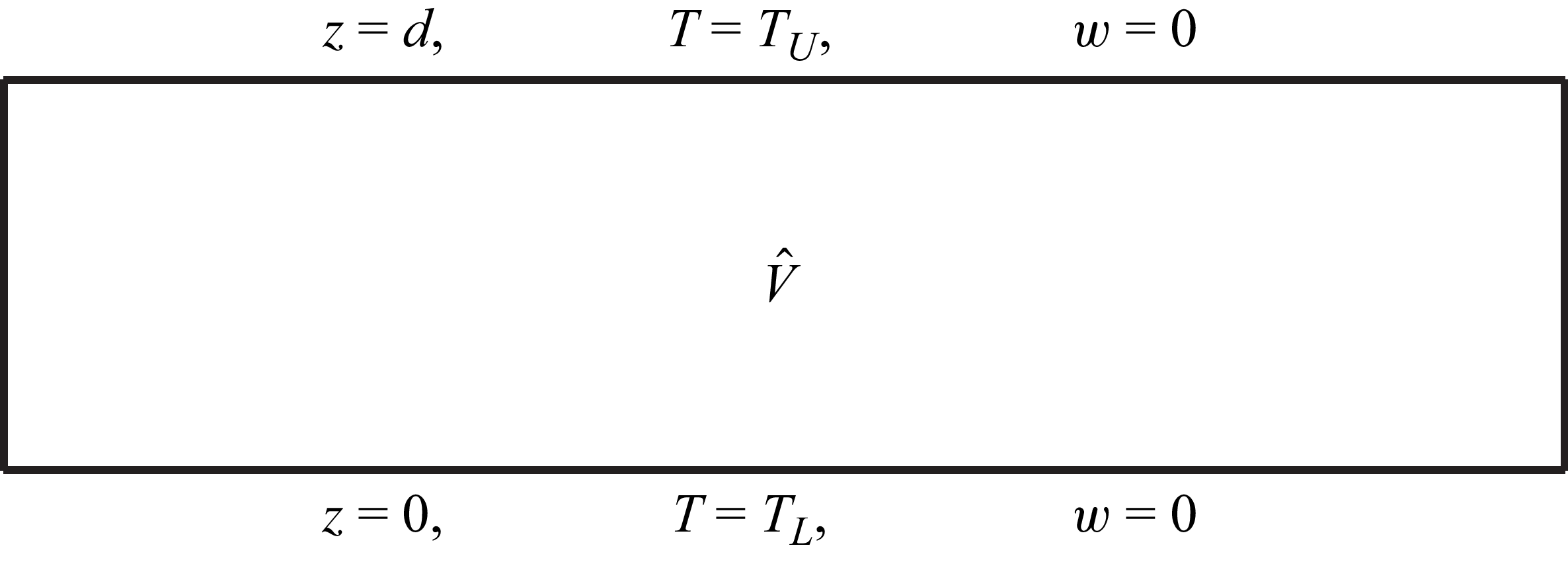
We are concerned with thermal convection in a non-dimensional horizontal layer of depth 1 and the convective motion will occur in a cellular structure the three-dimensional cell of which we denote by $V$ , which is the non-dimensional version of the dimensional cell $\hat V$ shown in Figure 1. A detailed discussion about possible cell shapes is contained in Chandrasekhar (Reference Chandrasekhar1981, p. 43–52). The inner product and norm in $L^2(V)$ are denoted by $(,\boldsymbol{\cdot },)$ and $\Vert \boldsymbol{\cdot }\Vert$ .

Figure 1.

Side view of a convection cell $\hat V$ . The top view is hexagonal. The vertical dashed lines indicate the corners of the cell. The region between the horizontal planes $z=0$ and $z=d$ is filled with a saturated porous material.

In this section we derive a fully nonlinear stability analysis for a solution to (3.3)–(3.7). In order to do this it is convenient to first transform (3.3)–(3.6) using an idea due to Oskolkov (Reference Oskolkov1988) in connection with a Jeffreys fluid model in viscoelasticity. Thus, we recall $\varOmega =q_{i,i}$ and we put $U=\Delta \theta$ . Then from (3.6) one may see that

(4.1) \begin{equation} \lambda \varOmega _t+\varOmega =-U-\mathfrak{J}U_t. \end{equation}

We now take the Laplace transform of (4.1) as is done in Zvyagin & Turbin (Reference Zvyagin and Turbin2010) for the viscoelastic Kelvin–Voigt fluid of order N; details of analogous but simpler calculations for Kelvin–Voigt fluids of order 1 or 2 are given in Straughan (Reference Straughan2026, p. 81–86).

After some rearrangement this leads to the equation

(4.2) \begin{equation} {\mathcal L}(\varOmega )=-{\mathcal L}(U) \left\{\frac {\mathfrak{J}}{\lambda }+\frac {(1-\mathfrak{J}/\lambda )}{(\lambda s+1)} \right\} +\frac {\lambda \varOmega (0)+\mathfrak{J}U(0)}{1+\lambda s}, \end{equation}

Where $\mathcal L$ denotes the Laplace transform and $s$ is the transform variable. Take the inverse transform using the shift and convolution theorems to derive, assuming fading memory,

(4.3) \begin{equation} \varOmega =-\frac {\mathfrak{J}}{\lambda }\,U -\Bigl (1-\frac {\mathfrak{J}}{\lambda }\Bigr )\frac {1}{\lambda }\int _0^tU(\eta )\exp \left[-\left(\frac {t-\eta }{\lambda }\right)\right]d\eta + \left[\varOmega (0)+\frac {\mathfrak{J}}{\lambda }\,U(0) \right]e^{-t/\lambda }. \end{equation}

Now we introduce the variable $W(\boldsymbol {x},t)$ by

(4.4) \begin{equation} W_t+\xi W=\theta , \end{equation}

and observe that $W(t)$ satisfies

(4.5) \begin{equation} \Delta W(t)=\Delta W(0)e^{-\xi t}+\int _0^te^{-\xi (t-s)}\Delta \theta (s){\rm d}s. \end{equation}

Now put

(4.6) \begin{equation} \alpha = \left(1-\frac {\mathfrak{J}}{\lambda }\right)\frac {1}{\lambda },\quad \xi =\frac {1}{\lambda },\quad \Delta W(0)=-\frac {[\varOmega (0)+\{\mathfrak{J}/\lambda \}\,U(0)]}{\alpha }. \end{equation}

Thanks to (4.5), (4.3) may be written as

(4.7) \begin{equation} \varOmega =-\frac {\mathfrak{J}}{\lambda }\,U-\alpha \Delta W. \end{equation}

Thus, we may rewrite (3.3)–(3.6) in the form

(4.8) \begin{align} 0=-\pi _{,i}-u_i+R\theta k_i,\quad u_{i,i}=0, \end{align}

(4.9) \begin{align} \theta _{,t}+u_i\theta _{,i}=Rw+\frac {\mathfrak{J}}{\lambda }\,\Delta \theta +\alpha \Delta W, \end{align}

(4.10) \begin{align} W_{,t}+\frac {1}{\lambda }\,W=\theta. \end{align}

The boundary conditions are

(4.11) \begin{equation} w=0,\quad \theta =0,\quad W=0,\quad \textrm {on}\quad z=0,1, \end{equation}

together with $(u_i,\theta ,W,\pi )$ being periodic in $x$ and $y$ .

The nonlinear stability analysis splits naturally into two cases. The first is when $\mathfrak{J}/\lambda \ge 1$ and so $\alpha \le 0$ . We now take $-\varDelta$ of (4.10) to derive the equation

(4.12) \begin{equation} -\Delta W_{,t}-\frac {1}{\lambda }\,\Delta W=-\Delta \theta . \end{equation}

Now write the system of partial differential equations (4.8), (4.9) and (4.12) in the form of an abstract equation

(4.13) \begin{equation} {\mathcal A}\,{\mathcal U}_t=M{\mathcal U}+N({\mathcal U}\,), \end{equation}

where ${\mathcal U}=(u,v,w,\theta ,W)^T$ , $\mathcal{A}=diag(0,0,0,1,-\Delta )$ , $N$ represents the nonlinear term $u_i\theta _{,i}$ and $M$ is the linear operator. Since $\alpha \le 0$ the linear operator in (4.13) is symmetric in the space $(L^2(V))^5$ and $({\mathcal U},N({\mathcal U}))=0$ in the inner product in that space. Thus, we know the growth rate is real as we have already established in the linear analysis, but due to a result of Galdi & Straughan (Reference Galdi and Straughan1985) we have a stronger result. This is that the linear instability boundary is identical to the global nonlinear stability one, which means that linear theory completely captures the physics of the onset of thermal convection.

The second case is when $\lambda \gt \mathfrak{J}$ and in this situation the linear operator $M$ which appears in (4.13) is not symmetric. There is a skew-symmetric part due to the terms $\alpha \Delta W$ and $-\Delta \theta$ , since now $\alpha \gt 0$ . However, we may derive an energy stability analysis by multiplying (4.8) by $u_i$ , (4.9) by $\theta$ , and (4.12) by $W$ , and integrating each over $V$ . Using the boundary conditions leads to the identities

(4.14) \begin{equation} \begin{aligned} &0=R(\theta ,w)-\Vert \boldsymbol {u}\Vert ^2,\\[5pt] &\frac {d}{\mathrm dt}\frac {1}{2}\Vert \theta \Vert ^2=R(\theta ,w)-\frac {\mathfrak{J}}{\lambda }\,\Vert \boldsymbol{\nabla }\theta \Vert ^2-\alpha (\boldsymbol{\nabla }W,\boldsymbol{\nabla }\theta ),\\[5pt] &\frac {d}{\mathrm dt}\frac {\alpha }{2}\,\Vert \boldsymbol{\nabla }W\Vert ^2=-\frac {\alpha }{\lambda }\,\Vert \boldsymbol{\nabla }W\Vert ^2+\alpha (\boldsymbol{\nabla }\theta ,\boldsymbol{\nabla }W). \end{aligned} \end{equation}

We add these equations together to derive

(4.15) \begin{equation} \frac {d}{\mathrm dt} \left(\frac {1}{2}\Vert \theta \Vert ^2+\frac {\alpha }{2}\,\Vert \boldsymbol{\nabla }W\Vert ^2 \right)= \textit{RI}-D-\frac {\alpha }{\lambda }\Vert \boldsymbol{\nabla }W\Vert ^2, \end{equation}

where $I=2(\theta ,w)$ and $D=\Vert \boldsymbol {u}\Vert ^2+(\mathfrak{J}/\lambda )\Vert \boldsymbol{\nabla }\theta \Vert ^2$ .

Define now $R_E$ by

(4.16) \begin{equation} \frac {1}{R_E}=\max _{H}\,\frac {I}{D}, \end{equation}

where $H$ is the space of admissible solutions, i.e.

(4.17) \begin{equation} H=\{u_i,\theta ,W\,\vert \, u_{i,i}=0, u_i\in L^2(V),\theta , W \in H^1_0(V),\,\textrm {plus}\,\,\textrm { periodicity},\,\,\textrm {in}\,\,x,y\}. \end{equation}

One then solves the maximum problem for $R_E$ and derives the Euler–Lagrange equations. In this way one finds

(4.18) \begin{equation} R_E^2=\frac {\mathfrak{J}}{\lambda }\,\frac {\varLambda ^2}{a^2}. \end{equation}

The details are similar to those in Straughan (Reference Straughan2026, p. 54–56). The critical threshold for nonlinear energy stability is found by minimising $R_E^2$ to find the threshold is $Ra_{\textit{energy}}=4\mathfrak{J}/\lambda \pi ^2$ and $a_E^2=\pi ^2$ . Thus, if $Ra\lt Ra_{\textit{energy}}$ from (4.15) one finds

(4.19) \begin{equation} \frac {d}{\mathrm dt} \left(\frac {1}{2}\Vert \theta \Vert ^2+\frac {\alpha }{2}\,\Vert \boldsymbol{\nabla }W\Vert ^2 \right )\leq -D \left(1-\frac {R}{R_E} \right)-\frac {\alpha }{\lambda }\Vert \boldsymbol{\nabla }W\Vert ^2, \end{equation}

and by use of Poincaré’s inequality $\Vert \theta \Vert$ and $\Vert \boldsymbol{\nabla }W\Vert$ decay exponentially in time. One shows that $\Vert \boldsymbol {u}\Vert$ has the same decay using (4.14) $_1$ . Thus a global nonlinear stability threshold is established.

Figure 2.

Graph of $Ra$ against the Maxwell coefficient $\lambda$ with fixed value of the Jeffrey coefficient $\mathfrak{J}$ . The dashed line indicates the stationary convection threshold, while the upper solid curve displays the oscillatory convection threshold and the lower curve shows the nonlinear energy stability limit.

We show the typical behaviour of the Rayleigh number thresholds in figure 2. Here, $\mathfrak{J}=0.1$ and $\lambda$ varies. The stationary convection limit is the dashed straight line and the upper dark curve shows the oscillatory convection threshold. The energy stability boundary is shown as the lower dark curve. It is possible sub-critical instability may occur in the region between the oscillatory convection and energy stability curves. In figure 2 the transition to stationary convection is at $\lambda =0.14627$ and the oscillatory curve drops from the value $Ra=39.4784$ at the transition to $Ra=11.4784$ when $\lambda =0.5$ . The energy stability curve varies from $Ra_{\textit{energy}}=26.9901$ at transition to $Ra_{\textit{energy}}=7.8957$ at $\lambda =0.5$ . The critical wavenumbers remain constant as $\lambda$ varies. We have also computed with $\mathfrak{J}=0.01$ and $\mathfrak{J}=0.5$ and the same qualitative behaviour is found. In this case the transitions occur when $\lambda =0.04702$ and $\lambda =0.54949,$ respectively.