1. Introduction
Submerged aquatic vegetation (SAV) plays an important role in many ecosystems (Costanza et al. Reference Costanza1997; Barbier et al. Reference Barbier, Hacker, Kennedy, Koch, Stier and Silliman2011). By filtering nutrients, producing oxygen (Wilcock et al. Reference Wilcock, Champion, Nagels and Croker1999) and capturing suspended sediment (e.g. Moore Reference Moore2004; Harvey et al. Reference Harvey, Noe, Larsen, Nowacki and McPhillips2011), SAV improves water quality. In addition, SAV communities protect shorelines from erosion by damping waves and storm surge (Barbier et al. Reference Barbier, Hacker, Kennedy, Koch, Stier and Silliman2011; Sutton-Grier, Wowk & Bamford Reference Sutton-Grier, Wowk and Bamford2015). It also supports biodiversity by providing habitat for commercially important marine species, promoting food security (Cullen-Unsworth & Unsworth Reference Cullen-Unsworth and Unsworth2013). Finally, the carbon sequestration rate of SAV ( $\textrm {gCm}^{-2}\ \textrm {yr}^{-1}$) is more than ten times greater than that in terrestrial ecosystems (Fourqurean et al. Reference Fourqurean2012). Because SAV benefits the environment in many ways, its protection and restoration is important to coastal ecosystems. Predicting the impact of canopies on the velocity field can improve the assessment of their ecosystem services and constrain restoration guidelines. For example, the in-canopy velocity is an important control on fine sediment retention and carbon sequestration in SAV (Dahl et al. Reference Dahl, Infantes, Clevesjö, Linderholm, Björk and Gullström2018). Carbon stock has also been shown to vary with distance from the canopy edge (Oreska, McGlathery & Porter Reference Oreska, McGlathery and Porter2017), reflecting the spatial scale of velocity adjustment. Further, restoration success increases with planting scale, with larger and denser plantings achieving a greater reduction in current, believed to provide a positive feedback to growth (van Katwijk et al. Reference van Katwijk, Bos, Hermus and Suykerbuyk2010, Reference van Katwijk2016).
Previous laboratory studies have described the fully developed velocity profile associated with a submerged canopy covering the full channel width, i.e. a two dimensional (2-D) velocity field (see the review in Nepf Reference Nepf2012). However, patchy distributions of SAV, with three-dimensional (3-D) velocity fields, are common in nature. For example, patches of the seagrass Cymodocea nodosa range from 1 m to 10 m (e.g. Duarte & Sand-Jensen Reference Duarte and Sand-Jensen1990). In addition, human impact and storms can fragment meadows into isolated patches (Montefalcone et al. Reference Montefalcone, Parravicini, Vacchi, Albertelli, Ferrari, Morri and Bianchi2010). The flow within a finite patch of vegetation cannot be described by the fully developed 2-D flow models (Folkard Reference Folkard2005; Sukhodolova & Sukhodolov Reference Sukhodolova and Sukhodolov2012). For vegetation patches of finite dimension, the evolution of velocity at the leading edge must be described. Previous studies have described flow development from the leading edge for emergent canopies of finite width (Rominger & Nepf Reference Rominger and Nepf2011; Zong & Nepf Reference Zong and Nepf2010) and submerged canopies that span the channel width (Chen, Jiang & Nepf Reference Chen, Jiang and Nepf2013), both of which represent 2-D flow evolution. When current meets the leading edge, a fraction of flow is diverted towards the open water. For 2-D meadows, flow diversion occurs in only one plane of flow. The present study developed an analytical model for canopies of both finite width and height, such that the flow is three dimensional. The model was validated using new laboratory experiments with both rigid and flexible canopies. Once validated, the model was used to explore a range of real field conditions.
2. Theoretical modelling
In the following sections we first derive an analytical solution for submerged canopies spanning the channel width, referred to as 2-D canopies. The solution is then expanded to submerged canopies of finite width, referred to as 3-D canopies. Finally, the analytical solutions are adapted for 2-D and 3-D flexible canopies.
2.1. Two-dimensional velocity evolution: submerged canopy of infinite width
When unidirectional flow encounters a 2-D submerged canopy, velocity decreases within the canopy ( $0\leqslant z < h$, with
 $h$ the canopy height), diverting flow to the region above the canopy, such that the velocity increases above the canopy (
 $h\leqslant z < H$, with
 $H$ the water depth; see figure 1). Note that
 $x$ and
 $z$ are the streamwise and vertical coordinates, respectively. Previous studies have used a two-layer model to characterize the fully developed flow over a submerged canopy (e.g. Konings, Katul & Thompson Reference Konings, Katul and Thompson2012; Chen et al. Reference Chen, Jiang and Nepf2013). The velocities within (
 $U_{1}(x$)) and above (
 $U_{2}(x$)) the canopy are assumed to be vertically uniform.
(a) Flow adjustment along a 2-D submerged canopy. Vertical grey bars denote the canopy elements. Dashed lines display the development of the vertical shear layer, which contains vortices generated by Kelvin–Helmholtz instability. Here  $\delta _{e}$ is the penetration length in the fully developed region, defined as the distance the shear layer vortices penetrate into the canopy;
 $X_D$ is the adjustment length. (b) Two-layer model with vertically uniform velocity within each layer. Within the adjustment region the vertically averaged velocity in the canopy and in the overflow are
 $U_{1}(x)$ and
 $U_{2}(x)$, respectively, and
 $U_{1f}$ and
 $U_{2f}$ are the velocities in the fully developed region, respectively. Here
 $U_{\infty }$ is the depth-averaged velocity upstream of the canopy.

For a submerged canopy of rigid cylinders, the fully developed, in-canopy velocity is described by (21) in Chen et al. (Reference Chen, Jiang and Nepf2013), i.e.
 \begin{equation} \frac{U_{1f}}{U_{\infty}} = \frac{1}{1-\dfrac{h}{H}\phi+\sqrt{\dfrac{C_{D}ah}{2C_{2Dim}(1-\phi)}\left(\dfrac{H-h}{H}\right)^{3}}}, \end{equation}
with cylinder diameter  $d$ and area density
 $n$ (
 $\textrm {cyl.}\ \textrm {m}^{-2}$), such that the solid volume fraction
 $\phi =({{\rm \pi} }/{4})nd^{2}$. Here
 $C_{D}$ is the drag coefficient on the canopy elements, and
 $a=nd$ is the frontal area per canopy volume. Equation (2.1) requires that the canopy drag is sufficient to produce a shear layer profile, which occurs for dimensionless meadow density
 $ah > 0.1$ (e.g. Belcher, Jerram & Hunt Reference Belcher, Jerram and Hunt2003; Nepf et al. Reference Nepf, Ghisalberti, White and Murphy2007). The coefficient
 $C_{2Dim}$ characterizes the turbulent momentum exchange between the two layers. The subscript ‘2Dim’ was chosen to represent 2-D canopies. Based on the roughness scaling, previous studies (e.g. Gioia & Bombardelli Reference Gioia and Bombardelli2001; Konings et al. Reference Konings, Katul and Thompson2012) have suggested that
 \begin{equation} C_{2Dim} = K_{c}\left(\frac{\delta_{e}}{H}\right)^{1/3}, \end{equation}
with  $\delta _{e}$ the penetration length, defined as the vertical extent of the shear layer within the canopy (figure 1a), and
 $K_{c}$ is an empirical constant which, for rigid canopies, is
 $K_{c}=0.07\pm 0.02$ (Chen et al. Reference Chen, Jiang and Nepf2013). The penetration length is inversely proportional to canopy drag,
 $\delta _{e}\sim (C_{D}a)^{-1}$ (Nepf et al. Reference Nepf, Ghisalberti, White and Murphy2007), with scale constant
 $0.3\pm 0.1$ determined from data across a wide range of physical scale
 $10^{-3}<(C_{D}a)^{-1}<10^{2}$, (Ghisalberti & Nepf Reference Ghisalberti and Nepf2009). The penetration length is also constrained by the water depth and the canopy height (Nepf & Vivoni Reference Nepf and Vivoni2000; Konings et al. Reference Konings, Katul and Thompson2012), such that
 \begin{equation} \delta_{e} = \min\left(\frac{0.3\pm 0.1}{C_{D}a}, H-h, h\right). \end{equation}
Chen et al. (Reference Chen, Jiang and Nepf2013) suggested that  $U_{1}(x)$ decays exponentially from the canopy leading edge over the adjustment length
 $X_{D}$, which is defined as the distance required for the in-canopy velocity to achieve 95 % of the transition from upstream
 $U_{\infty }$ to fully developed
 $U_{1f}$, i.e.
 \begin{equation} \left\{\begin{array}{@{}ll} U_{1}(x) = U_{1f} + (U_{\infty}-U_{1f})\,\textrm{e}^{-{3x}/{X_{D}}}, \\ \dfrac{X_{D}}{L_{c}} = A_{1}[1+A_{2}]C_{D}ah, \end{array} \right. \end{equation}
in which  $L_{c} =({2(1-\phi )})/{C_{D}a}$ is the canopy drag length scale (Belcher et al. Reference Belcher, Jerram and Hunt2003). Using the empirical coefficients determined by Chen et al. (Reference Chen, Jiang and Nepf2013),
 $A_{1}=1.5\pm 0.2$ and
 $A_{2}=2.3\pm 0.2$, (2.4) can be written as
 \begin{equation} \frac{X_{D}}{h} = (6.9\pm 1.1)(1-\phi) + \frac{3.0\pm 0.4}{C_{D}ah}(1-\phi). \end{equation}
The exponential decay model works well for sparse canopies, but it overestimates the velocity for dense canopies ( $ah > 1.4$, figure 15 in Chen et al. Reference Chen, Jiang and Nepf2013). In the present study, rather than assuming exponential decay, an analytical solution to
 $U_{1} (x)$ was derived, appropriate for any density
 $ah > 0.1$. The continuity and layer-averaged momentum equations in the developing region can be written as follows (see also (18)–(20) in Chen et al. Reference Chen, Jiang and Nepf2013).
Continuity:
 \begin{equation} U_{1}(x)h(1-\phi) + U_{2}(x)(H-h) = U_{\infty} H. \end{equation}
Conservation of momentum in the canopy layer:
 \begin{align} \rho\left[U_{1}(x)\frac{\partial U_{1}}{\partial x}+W_{1}(x)\left(\frac{\partial U}{\partial z}\right)_{1}\right]h &= \rho gh\frac{\partial H}{\partial x} - \frac{\rho C_{D}ah}{2(1-\phi)}U_{1}(x)^{2} \nonumber\\ &\quad + \rho C_{2Dim}(U_{2}(x) - U_{1}(x))^{2}. \end{align}
Conservation of momentum in the overflow layer:
 \begin{align} \rho\left[U_{2}(x)\frac{\partial U_{2}}{\partial x}+W_{2}(x)\left(\frac{\partial U}{\partial z}\right)_{2}\right](H-h) = \rho g(H-h)\frac{\partial H}{\partial x} - \rho C_{2Dim}(U_{2}(x)-U_{1}(x))^{2} . \end{align}
The vertical velocity ( $W$) and vertical gradient of
 $U({\partial U}/{\partial z})$ at the shared interface (
 $z=h$) must be the same, such that
 $W_{1}(x)=W_{2}(x)$ and
 $({\partial U}/{\partial z})_{1}=({\partial U}/{\partial z})_{2}$. The vertical transport and the pressure terms can be cancelled with the manipulation ((2.7) and (2.8)
 $\times \,h/({H-h})$), resulting in
 \begin{align} \left[U_{1}(x)\frac{\partial U_{1}(x)}{\partial x} - U_{2}(x)\frac{\partial U_{2}(x)}{\partial x}\right] h = C_{2Dim}(U_{2}(x) - U_{1}(x))^{2}\frac{H}{H-h} - \frac{C_{D}ah}{2(1-\phi)}U_{1}(x)^{2}. \end{align}
Combining (2.6) and (2.9), an expression for  $U_{1} (x)$ was determined, i.e.
 \begin{align} &\frac{\partial U_{1}(x)}{\partial x}h\frac{U_{1}(x)[(H-h)^{2}-(1-\phi)^{2}h^{2}]+U_{\infty}Hh(1-\phi)}{(H-h)^{2}} \nonumber\\ &\quad =C_{2Dim}\left[U_{\infty}-U_{1}(x)\left(1-\frac{h}{H}\phi\right)\right]^{2} \left(\frac{H}{H-h}\right)^{2}\nonumber\\ &\qquad - \frac{C_{D}ah}{2(1-\phi)}U_{1}(x)^{2} . \end{align}
In the fully developed region,  ${\partial U_{1}(x)}/{\partial x}=0$ and (2.10) correctly reverts to (2.1). The analytical solution to (2.10) was derived as follows. Let
 \begin{equation} \left\{\begin{array}{@{}l} \alpha = \dfrac{[(H-h)^{2} - (1-\phi)^{2}h^{2}]h}{(H-h)^{2}}, \\ \beta = C_{2Dim}\left(\dfrac{H}{H-h}\right)^{3} \left(1-\dfrac{h}{H}\phi\right)^{2}-\dfrac{C_{D}ah}{2(1-\phi)}, \\ A' = \dfrac{Hh(1-\phi)}{(H-h)^{2} - (1-\phi)^{2}h^{2}}U_{\infty}, \\ B' = \dfrac{-2\left(1-\dfrac{h}{H}\phi\right)}{\left(1-\dfrac{h}{H}\phi\right)^{2} - \dfrac{C_{D}ah}{2C(1-\phi)}\left(\dfrac{H-h}{H}\right)^{3}}U_{\infty}, \\ C' = \dfrac{1}{\left(1-\dfrac{h}{H}\phi\right)^{2} - \dfrac{C_{D}ah}{2C(1-\phi)}\left(\dfrac{H-h}{H}\right)^{3}}U_{\infty}^{2}, \end{array} \right. \end{equation}
and substitute (2.11) into (2.10), we get
 \begin{equation} \frac{\alpha}{\beta}\frac{U_{1}(x)+A'}{U_{1}(x)^{2}+B'U_{1}(x)+C'}\,\textrm{d} U_{1}(x) = {\textrm{d} x} . \end{equation}
Integrating (2.12) yields
 \begin{equation} \left\{\begin{array}{@{}l} f(U) = \displaystyle\int\dfrac{U+A'}{U^{2}+B'U+C'}\,\textrm{d}U = \dfrac{2A'-B'}{\sqrt{4C'-B'^{2}}}\arctan\dfrac{B'+2U}{\sqrt{4C'-B'^{2}}} \\ \qquad \quad + \dfrac{1}{2}\ln(U^{2}+B'U+C'),\\ f(U_{1}(x)) - f(U_{\infty}) = \dfrac{\beta}{\alpha}x, \end{array} \right.. \end{equation}
Note that (2.11) can be simplified if  $\phi \ll 1$. The simplified expression is shown in Appendix A.1. With
 ${\partial U_{1}(x)}/{\partial x}$ given in (2.10), forward Euler's method was used to compute
 $U_{1} (x)$ with the initial condition
 $U_{1}(x=0)=U_{\infty }$, which is justified in § 4.4.
A scale analysis of (2.7) was used to provide a framework for the dependence of  $X_{D}$ on pressure, drag and shear forcing terms. First,
 $U_{2}$ was scaled with
 $U_{\infty }$, and
 $(U_{2}-U_{1}) = ({H}/({H-h}))(U_{\infty }-U_{1})\sim ({H}/({H-h}))U_{\infty }$. Second, the distance from the leading edge,
 $x$, was scaled with
 $X_{D}$. Third, based on previous studies (e.g. Rominger & Nepf Reference Rominger and Nepf2011), the pressure terms
 $\rho gh({\partial H}/{\partial x})$ scale with
 ${\rho U_{\infty }^{2}C_{D}ah}/{X_{D}}$. Finally,
 $\phi$ was neglected for simplicity. With these scales, (2.7) yields
 \begin{equation} \left.\begin{gathered} -\frac{U_{\infty}^{2}}{X_{D}} \sim \frac{C_{D}ahU_{\infty}^{2}}{X_{D}}+ C_{2Dim}\frac{U_{\infty}^{2}}{h}\left(\frac{H}{H-h}\right)^{2}-C_{D}aU_{\infty}^{2}, \\ \qquad\quad pressure\qquad \qquad \qquad shear\qquad\qquad drag\\ \frac{X_{D}}{h}\sim\frac{C_{D}ah+1}{C_{D}ah-C_{2Dim}\left(\dfrac{H}{H-h}\right)^{2}}. \end{gathered}\right\}\end{equation}
This shows that the inclusion of the turbulent shear stress at the top of the canopy, which was excluded by Chen et al. (Reference Chen, Jiang and Nepf2013), extends the adjustment length, which is consistent with the tendency to accelerate the velocity within the canopy. Note that when the drag term is much greater than the shear term, (2.14) reverts to the form proposed by Chen et al. (Reference Chen, Jiang and Nepf2013), shown in (2.5).
2.2. Three-dimensional velocity evolution: submerged canopy of finite width
For 3-D canopies, the flow was separated into the canopy region, with velocity  $U_{1,3D} (x)$, and the open-channel (outer) region, with velocity
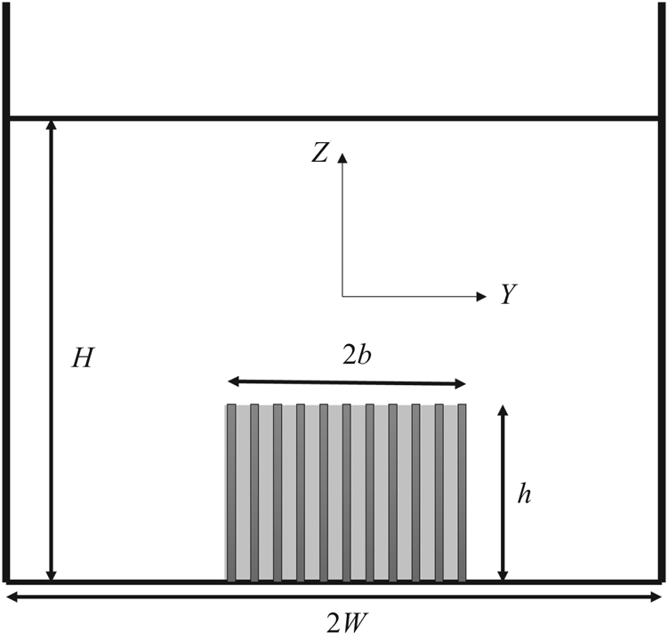
 $U_{2,3D} (x)$, with the averaging now defined over the fraction of cross-sectional area occupied by the canopy (grey in figure 2) and outside the canopy (white in figure 2), respectively. Since the model assumes a spatially uniform velocity outside the canopy,
 $U_{2,3D} (x)$, the accuracy of the model will diminish if the edges of the canopy are too close to the boundaries (
 ${h}/{H}\approx 1$ or
 ${b}/{W}\approx 1$). In that case, the flow velocity on the top of the canopy might be significantly different from that in regions next to the lateral interfaces. The analytical solution in the following is strictly valid for cases with small
 ${h}/{H}$ and
 ${b}/{W}$. In our experiments, different values of
 ${h}/{H}$ (
 ${h_{d}}/{H}$ for 3-D flexible canopies) and
 ${b}/{W}$ were considered to explore the range of validity of the 3-D analytical model. For
 ${h_{d}}/{H}$ and
 ${b}/{W}$ as large as 0.52 and 0.51, the velocity in the regions above and adjacent to the canopy are comparable, supporting the model assumption of a spatially uniform velocity outside the canopy.
Cross-section of a channel with a submerged canopy of finite width  $2b$ (3-D canopy). The channel width is
 $2W$. The canopy, shown with grey shading, has velocity
 $U_{1,3D} (x)$), and the unobstructed outer flow region, shown in white, has velocity
 $U_{2,3D} (x)$. The vertical bars denote canopy elements. The canopy height is
 $h$. The water depth is
 $H$.

For the 3-D submerged canopy, three interfaces must be considered, introducing new terms into the momentum equations. The additional subscript ‘3D’ was added to distinguish this as the 3-D solution.
Continuity:
 \begin{equation} U_{1,3D}(x)bh(1-\phi) + U_{2,3D}(x)(WH-bh) = U_{\infty}WH. \end{equation}
Conservation of momentum in the canopy region (region 1):
 \begin{align} &\rho\left[U_{1,3D}(x)\frac{\partial U_{1}(x)}{\partial x} + V_{1,3D}(x)\left(\frac{\partial U}{\partial y}\right)_{1} + W_{1,3D}(x)\left(\frac{\partial U}{\partial z}\right)_{1}\right]bh \nonumber\\ &\quad =\rho gbh\frac{\partial H}{\partial x} - \frac{\rho C_{D}ahb}{2(1-\phi)}U_{1,3D}(x)^{2} + \rho C_{3Dim}(b+h)[U_{2,3D}(x) - U_{1,3D}(x)]^{2} . \end{align}
Conservation of momentum outside the canopy (region 2):
 \begin{align} & \rho\left[U_{2,3D}(x)\frac{\partial U_{2}(x)}{\partial x} + V_{2,3D}(x)\left(\frac{\partial U}{\partial y}\right)_{2} + W_{2,3D}(x)\left(\frac{\partial U}{\partial z}\right)_{2}\right] (WH - bh) \nonumber\\ &\quad =\rho g(WH-bh)\frac{\partial H}{\partial x} - \rho C_{3Dim}(b+h)[U_{2,3D}(x) - U_{1,3D}(x)]^{2}. \end{align}
Similar to 2-D canopies, the advective transport of momentum between the two zones, represented by the second and third terms of (2.16) and (2.17), must be equal at the interface between the two zones. The vertical velocity ( $W$) and vertical gradient of
 $U({\partial U}/{\partial z})$ at the shared interface (
 $z = h$) must be the same,
 $W_{1,3D}(x)=W_{2,3D}(x)$ and
 $({\partial U}/{\partial z})_{1}=({\partial U}/{\partial z})_{2}$. Similarly, lateral velocity and its lateral gradient are continuous across the boundary between the two regions, such that
 $V_{1,3D}(x)=V_{2,3D}(x)$ and
 $({\partial U}/{\partial y})_{1}=({\partial U}/{\partial y})_{2}$. Then, the advective transport terms and the pressure terms can be cancelled with the manipulation ((2.16) and (2.17)
 $\times \,bh/({WH-bh})$).
Here,  $C_{3Dim}$ is the coefficient that characterizes the turbulent momentum exchange between the canopy and outer flow. The 3-D canopy has three interfaces with the outer flow, two along the side boundaries and one at the top. The penetration length scale,
 $\delta _{e}$, and the coefficient,
 $K_{c}$, were assumed to be the same on every interface. This is supported by data in White & Nepf (Reference White and Nepf2008), who considered momentum exchange at the lateral edge of a cylinder array. They found
 $\delta _{e}\approx 0.5(C_{D}a)^{-1}$, which is close to (2.3), and
 $K_{c}=0.06\pm 0.03$ (based on table 1 of that paper), which is similar to the value observed at the top interface (
 $K_{c}=0.07\pm 0.02$, Chen et al. Reference Chen, Jiang and Nepf2013), so that the application of a single roughness on all three interfaces of a 3-D canopy was reasonable. Here,
 $K_{c}=0.07\pm 0.02$ was used for all interfaces. To represent the average dimension of the outer flow, the water depth,
 $H$, was replaced with the hydraulic radius,
 $R$, defined as the channel cross-section divided by its wetted perimeter,
 $R=(({H\times 2W})/({2H+2W}))={HW}/({H+W})$, and then (2.2) becomes
 \begin{equation} C_{3Dim} = K_{c}\left(\frac{\delta_{e}}{R}\right)^{1/3}. \end{equation}
Note that as the channel width ( $2W$) approaches infinity, (2.18) appropriately reverts (2.2). The penetration length is also constrained by the water depth, the canopy height, the channel width and the canopy width. Similar to (2.3), for 3-D canopies,
 \begin{equation} \delta_{e}=\min{\left(\frac{0.3\pm 0.1}{C_{D}a},H-h,h,W-b,b\right)}. \end{equation}
Finally, combining (2.15), (2.16) and (2.17), we get
 \begin{align} & \frac{\textrm{d} U_{1,3D}(x)}{\textrm{d} x}bh\frac{U_{1,3D}(x)[(WH-bh)^{2}-(1-\phi)^{2}(bh)^{2}]+ U_{\infty}WHbh(1-\phi)}{(WH-bh)^{3}} \nonumber\\ &\quad = C_{3Dim}(b+h)\left[U_{\infty}-U_{1,3D}(x)\left(1-\frac{bh}{WH}\phi\right)\right]^{2} \left(\frac{WH}{WH-bh}\right)^{3} \nonumber\\ &\qquad - \frac{C_{D}abh}{2(1-\phi)}U_{1,3D}(x)^{2}. \end{align}
In the fully developed region,  ${\textrm {d} U_{1,3D} (x)}/{\textrm {d} x}=0$, from which (2.20) predicts the fully developed in-canopy velocity,
 $U_{1f,3D}$,
 \begin{equation} \frac{U_{1f,3D}}{U_{\infty}} = \frac{1}{1-\dfrac{bh}{WH}\phi+\sqrt{\dfrac{C_{D}abh}{2C_{3Dim}(b+h)(1-\phi)}\left(\dfrac{WH-bh}{WH}\right)^{3}}}. \end{equation}
The complete analytical solution to (2.20) is shown in Appendix A.2.
2.3. Flexible canopies
Some canopies, such as a seagrass meadow, consist of flexible blades which bend in response to flow. The bending of blades, called reconfiguration, can be described by two dimensionless parameters (e.g. Luhar & Nepf Reference Luhar and Nepf2011). The Cauchy number ( $Ca$, (2.22)) is the ratio of hydrodynamic drag to the restoring force due to blade stiffness, and the buoyancy parameter (
 $B$, (2.23)) is the ratio of buoyancy force to the restoring force, i.e.
 \begin{gather} Ca = \frac{\frac{1}{2}C_{D}\rho w_{b}\,\textrm{d}U^{2}l^{3}}{EI}, \end{gather}
 \begin{gather}B = \frac{\Delta\rho g\,\textrm{d}tl^{3}}{EI}. \end{gather}
Here,  $w_{b}$ and
 $t$ are the blade width and thickness, respectively,
 $\rho$ is the density of water,
 $U$ is the velocity acting on the blade,
 $\Delta \rho$ is the difference in density between the water and the blade,
 $E$ is the Young's modulus and
 $I={w_{b}t^{3}}/{12}$ is the bending moment of inertia. The vertical distance between the blade tip and the blade base is called the deflected blade height,
 $h_{d,b}$. Combining experiments and simulation, Luhar et al. (Reference Luhar, Infantes, Orfila, Terrados and Nepf2013) described the deflected blade height (4) of individual artificial seagrass blades under unidirectional currents as a function of
 $Ca$ and
 $B$, i.e.
 \begin{equation} \frac{h_{d,b}}{l} = 1 - \frac{1-Ca^{-{1}/{4}}}{1+Ca^{-{3}/{5}}(4+B^{{3}/{5}})+Ca^{{-}2}(8+B^{2})}. \end{equation}
Furthermore, the drag on a flexible blade can be described by an effective blade length,  $l_{e,b}$, which is the length of a rigid blade that experiences the same drag as a flexible blade of length
 $l$. Reconfiguration reduces drag, such that
 $l_{e,b} < l$. Combining experiments and simulation, Luhar & Nepf (Reference Luhar and Nepf2011, (16)) described
 \begin{equation} \frac{l_{e,b}}{l} = 1-\frac{1-0.9Ca^{-{1}/{3}}}{1+Ca^{{2}/{3}}(8+B^{{3}/{2}})}. \end{equation}
For the flexible canopies, the deflected canopy height,  $h_{d}$, was calculated as the sum of the deflected blade height,
 $h_{d,b}$ (by (2.24)), and the sheath height,
 $l_{s}$, i.e.
 \begin{equation} h_{d} = h_{d,b} + l_{s}. \end{equation}
The flexible canopy drag was defined as  $C_{D}al_{e} = C_{D}nA_{f,e}$, with
 $A_{f,e}$ the effective frontal area per plant with deflected blades,
 \begin{equation} \left.\begin{gathered} C_{D}al_{e} = C_{D}nA_{f,e} = n(6C_{D,plate}l_{e,b}b + C_{D,cylinder}l_{s}d),\\ \qquad\qquad\qquad\qquad\qquad blades\qquad\qquad sheath \end{gathered}\right\} \end{equation}
with  $l_{e,b}$ estimated from (2.25).
We propose (and later test) that flow development in a flexible canopy can be described by the governing equations developed above, with two adjustments. First, in the terms related to canopy geometry, the canopy height,  $h$, was replaced by the deflected height,
 $h_{d}$. Second, the canopy drag (
 $C_{D} ah$) is replaced by
 $C_{D}al_{e}$, defined in (2.27). Making these changes in (2.10) and (2.20), the canopy velocity in flexible 2-D (
 $U_{1}$) and 3-D (
 $U_{1,3D}$) canopies, can be expressed, respectively, as
 \begin{align} &\frac{\textrm{d} U_{1}(x)}{\textrm{d} x}h_{d}(x)\frac{U_{1}(x)[(H-h_{d}(x))^{2}-(1-\phi)^{2}h_{d}(x)^{2}]+U_{\infty}Hh_{d}(x)(1-\phi)}{(H-h_{d}(x))^{2}} \nonumber\\ &\quad = C\left[U_{\infty}-U_{1}(x)\left(1-\frac{h_{d}(x)}{H}\phi\right)\right]^{2} \left(\frac{H}{H-h_{d}(x)}\right)^{3} - \frac{C_{D}al_{e}(x)}{2(1-\phi)}U_{1}(x)^{2}, \end{align}
 \begin{align} &\frac{\textrm{d} U_{1,3D}(x)}{\textrm{d} x}bh_{d}(x) \frac{U_{1,3D}(x)[(WH-bh_{d})^{2}-(1-\phi)^{2}(bh_{d}(x))^{2}]+U_{\infty}WHbh_{d}(x)(1-\phi)}{(WH-bh_{d}(x))^{2}} \nonumber\\ &\quad = C_{3Dim}(b+h_{d}(x))\left[U_{\infty}-U_{1,3D}(x)\left(1-\frac{bh_{d}(x)}{WH}\phi\right)\right]^{2} \left(\frac{WH-bh_{d}(x)}{WH}\right)^{3}\nonumber\\ &\qquad - \frac{C_{D}abl_{e}(x)}{2(1-\phi)}. \end{align}
Because  $h_{d} (x)$ and
 $l_{e} (x)$ are functions of the velocity (through
 $Ca$), forward Euler's method was used to compute
 $U_{1} (x)$ and
 $U_{1,3D} (x)$. The computation of the flow development is described in Appendix A.3. In the fully developed region the deflected height and the effective length become constant (
 $h_{d} (x)=h_{df}$,
 $l_{e} (x)=l_{ef}$). Also,
 ${\partial U_{1}(x)}/{\partial x}=0$ and
 ${U_{1,3D} (x)}/{\partial x}=0$, leading to
 \begin{gather} {\rm 2-D\; flexible\; canopy:} \frac{U_{1f}}{U_{\infty}} = \frac{1}{1-\dfrac{h_{df}}{H}\phi + \sqrt{\dfrac{C_{D}al_{ef}}{2C_{2Dim}(1-\phi)}\left(\dfrac{H-h_{df}}{H}\right)^{3}}}, \end{gather}
 \begin{gather} {\rm 3-D\; flexible\; canopy:} \frac{U_{1f,3D}}{U_{\infty}} = \frac{1}{1-\dfrac{bh_{df}}{WH}\phi + \sqrt{\dfrac{C_{D}abl_{ef}}{2C_{3Dim}(b+h_{df})(1-\phi)}\left(\dfrac{WH-bh_{df}}{WH}\right)^{3}}}, \end{gather}
in which  $h_{df}$ and
 $l_{ef}$ denote the deflected height and the effective length in the fully developed region. Because
 $h_{df}$ and
 $l_{ef}$ depend on the flow velocity, (2.30) and (2.31) were applied in an iterative fashion to calculate
 $U_{1f}$ and
 $U_{1f,3D}$.
2.4. Unbounded domain
Field conditions are better represented by a canopy of finite width within an unbounded domain, corresponding to  $W \gg b$, or
 ${b}/{W}\sim 0$, for which (2.21) reduces to
 \begin{equation} \frac{U_{1f,3D}}{U_{\infty}} = \frac{1}{1+\sqrt{\dfrac{C_{D}ahb}{2C_{3Dim}(b+h)(1-\phi)}}} . \end{equation}
For  $b\gg h$, the geometry of the canopy could be considered to approach that of a 2-D canopy. With these limits, (2.32) reduced to
 \begin{equation} {\rm 3-D\; canopy:} \frac{U_{1f,3D}}{U_{\infty}} = \frac{1}{1+\sqrt{\dfrac{C_{D}ah}{2C_{3Dim}(1-\phi)}}}, \end{equation}
which differed from the original 2-D solution, repeated here for comparison;
 \begin{equation}{\rm 2-D\; canopy:} \frac{U_{1f}}{U_{\infty}} = \frac{1}{1-\dfrac{h}{H}\phi+\sqrt{\dfrac{C_{D}ah}{2C_{2Dim}(1-\phi)}\left(\dfrac{H-h}{H}\right)^{3}}}. \end{equation}
The difference arises from the assumed confinement of the flow domain. A channel-spanning 2-D canopy (2.34) is confined by the channel walls, such that continuity required that flow diverted out of the canopy must be incorporated into the overflow, such that the overflow velocity ( $U_{2}$) increased as the flow within the canopy (
 $U_{1}$) decreased. For 3-D canopies, when
 $W\gg b$ and
 $b\gg h$, only a small portion of the channel is occupied by the canopy, such that the flow velocity outside the canopy is still approximately equal to
 $U_{\infty }$.
3. Methods and materials
3.1. Model canopies
Canopies were constructed from model plants held in a staggered array. The rigid canopies consisted of rigid cylinders 6.4 mm in diameter ( $d$), 7 cm tall (
 $h$), with area density
 $n$ (
 $\textrm {cyl}.\ \textrm {m}^{-2}$). The dimensionless canopy density
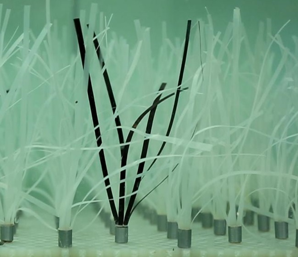
 $ah = ndh$. The flexible canopy consisted of model plants that were geometrically and dynamically similar to the seagrass Zostera marina (figure 3). Each plant consisted of six LDPE (low-density polyethylene) blades (
 $\textrm {density}= 920\ \textrm {kg}\ \textrm {m}^{-3}$;
 $E = 3\times 10^{8}\ \textrm {Pa}$) with length
 $l_{b}=13$ cm, width
 $w_{b}=3$ mm and thickness
 $t=0.1$ mm, attached to a rigid, circular cylinder, representing the plant sheath, which is rigid. The sheath protruded
 $l_{s}=1$ cm above the baseboard. The frontal area of each model plant was
 $A_{f}=l_{s}d + 6w_{b}l_{b}$ with
 $d=6.4$ mm. With
 $n$ plants per
 $\textrm {m}^{2}$,
 $ah=nA_{f}$. The cylinder (or plant) density (
 $n$), dimensionless canopy density (
 $ah$) and channel-average flow velocity (
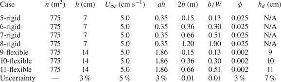
 $U_{\infty }$) are summarized in table 1 (2-D canopies) and table 2 (3-D canopies).
Side view of recirculating water channel with 8 m long submerged canopy that covered the channel width (2-D canopy). Figure is not to scale. Velocity measured with Nortek Vectrino along the centreline of the channel.

Experimental conditions for 2-D canopies. Here  $n =$ shoots per bed area; full canopy height,
 $h$; and deflected height,
 $h_{d}$, for flexible canopies only. For the rigid plants,
 $ah=ndh$ and
 $\phi ={\rm \pi} /4 nd^{2}$. For the flexible plants, the frontal area of each flexible plant was
 $A_{f}=l_{s}d+6w_{b}l_{b}$,
 $ah=nA_{f}$ and
 $\phi =({l_{s}({{\rm \pi} }/{4})nd^{2}+6l_{b}nbt})/({l_{s}+l_{b}})$. Each flexible plant had six blades, so that
 $n=520\ \textrm {plants}\ \textrm {m}^{-2}$ corresponded to
 $3120\ \textrm {blades}\ \textrm {m}^{-2}$.

Experimental conditions for 3-D submerged canopies. Here  $n=\text {shoots}$ per bed area; full canopy height,
 $h$, canopy width,
 $2b$; channel width
 $2W=120$ cm; and deflected height,
 $h_{d}$, for flexible canopies only. For rigid plants,
 $ah = ndh$ and
 $\phi =({{\rm \pi} }{4})nd^{2}$. For the flexible plants, the frontal area per plant was
 $A_{f}=l_{s}d+6w_{b}l_{b}$,
 $ah=nA_{f}$ and
 $\phi =({l_{s}({{\rm \pi} }/{4})nd^{2}+6l_{b}nbt})/({l_{s}+l_{b}})$. Each flexible plant had six blades, so that
 $n = 775\ \textrm {plants}\ \textrm {m}^{-2}$ corresponded to
 $4650\ \textrm {blades}\ \textrm {m}^{-2}$.

3.2. Two-dimensional canopies
Two-dimensional canopy experiments were conducted in a 24 m long, 38 cm wide recirculating water channel (figure 4). The water depth was  $H = 36$ cm. The model canopy was 8 m long. Vertical profiles of velocity were measured using a Nortek Vectrino, which was placed between two adjacent model plants at mid-width of the channel. Previous studies using staggered arrays have shown that the mean velocity at this point was within 5 % of the lateral average across a 2-D canopy (see figure 2 in Chen et al. Reference Chen, Jiang and Nepf2013). Vertical profiles were measured at multiple streamwise locations starting upstream of the canopy,
 $x=-3h$ to
 $x=84h$, and with 1 cm intervals from the bed (
 $z = 0$). For each measurement, velocity was collected for
 $T=6$ min at a sampling rate of 200 Hz. The depth-averaged velocity upstream of the canopy,
 $U_{\infty }$, was determined from a vertical profile measured at 1 m upstream of the leading edge.
Canopy of flexible plants, dynamically and geometrically similar to Z. marina. Each plant consists of six LDPE blades attached to a rigid sheath (grey in image). One plant is painted in black to enhance visualization.

3.3. Three-dimensional canopies
Submerged canopies of finite width were constructed in a 16 m long and 1.2 m wide recirculating channel. The water depth was  $H = 20$ cm. The model canopies were 2.4 m long. Four different canopy widths (
 $2b$) were constructed (table 2, figure 5). Velocity was measured at multiple distances from the leading edge,
 $x= 1.5h$ to
 $x=7.4h$. At each streamwise position, the velocity was measured at 18 positions in a grid of six lateral positions and three vertical positions. The lateral distribution of measurement points in the canopy are shown in figure 6 for different arrays. The vertical positions were 2.5, 4 and 6 cm for rigid canopies and 3, 6 and 8 cm for flexible canopies. The measurement positions were mid-way between adjacent rows and columns. The average of the 18 positions defined the in-canopy velocity,
 $U_{1,3D}$.
Recirculating channel with a submerged canopy of finite width ( $2b$) less than the channel width (
 $2W = 1.2$ m). Shaded region denotes the canopy, located at the channel centre. (a) Side view; (b) top view; (c) front view. Not to scale.

Top view of canopy, with plant positions shown with grey circles. Blue circles denote velocity measurement points located mid-way between adjacent rows and columns of plants. At each blue dot, velocity was measured at three vertical positions,  $z=2.5$,
 $4$ and
 $6$ cm for rigid canopies and
 $z=3$,
 $6$ and
 $8$ cm for flexible canopies. The canopy width is
 $2b$. (a) Case 5 and 9, velocity measured at
 $y=\pm \frac {5}{6}b$,
 $\pm \frac {1}{2}b$,
 $\pm \frac {1}{6}b$. (b) Case 6 and 10,
 $y=\pm \frac {13}{14} b$,
 $\pm \frac {1}{2}b$,
 $\pm \frac {1}{14}b$. (c) Case 7 and 11,
 $y=\pm \frac {25}{26} b$,
 $\pm \frac {15}{26} b$,
 $\pm \frac {5}{26} b$. The black dashed lines denote the channel and canopy centreline (
 $y = 0$).

3.4. Estimation of deflected height
The deflected height was measured using images from a digital camera looking through the side of the channel. A black background was taped to the opposite channel wall. Ten images were taken at one-second intervals and used to estimate deflected height at nine positions along the meadow. The measured deflected height was estimated from the average across all the ten photos, and uncertainty was calculated as the standard deviation.
3.5. Validation of the analytical model
The initial adjustment length,  $X_{D}$, was defined as the distance from the leading edge to the point at which the canopy velocity reached the 95 % transition from the upstream velocity
 $U_{\infty }$ to fully developed velocity
 $U_{1f}$, i.e.
 $U_{1} (X_{D})=0.05(U_{\infty }-U_{1f} )+U_{1f}$. It was estimated from both the measured and predicted velocity. The measured
 $X_{D}$ was interpolated between the measured velocities closest to
 $U_{1}(X_{D})$. For the prediction, the rigid element drag coefficient,
 $C_{D}$, was estimated for cylinders from the numerical study of staggered arrays by Etminan, Lowe & Ghisalberti (Reference Etminan, Lowe and Ghisalberti2017), and for flat plates, representing the blades, from Ellington (Reference Ellington1991),
 \begin{equation} \left\{\begin{array}{@{}l} C_{D,cylinder} = 1 + Re_{c}^{2/3}, \\ C_{D,plate} = 1.95 + \dfrac{50}{Re_{w}}, \end{array} \right. \end{equation}
in which the cylinder Reynolds number  $Re_{c}=({U_{1}d}/{\nu })(({1-\phi })/({1-\sqrt {{2\phi }/{{\rm \pi} }}}))$ and the plate Reynolds number
 $Re_{w}={U_{1}w_{b}}/{\nu }$. Since velocity and, thus, Reynolds number, changed along the canopy,
 $C_{D}$ and its uncertainty were evaluated as follows. First,
 $C_{D}$ was calculated using the velocity
 $U_{\infty }$, resulting in
 $C_{D} (U_{\infty })$, which was then used to make a preliminary prediction of
 $U_{1f}$. Second, we used
 $U_{1f}$ to calculate the drag coefficient in the fully developed region,
 $C_{D} (U_{1f})$. Finally, a mean drag coefficient was calculated using
 $({U_{\infty }+U_{1f}})/{2}$ as the representative velocity. The uncertainty in
 $C_{D}$ was evaluated from the maximum,
 $C_{D} (U_{1f})$, and minimum,
 $C_{D} (U_{\infty })$. Finally,
 $U_{1f}$ was recalculated using
 $C_{D}(({U_{\infty }+U_{1f}})/{2})$, and the resulting
 $U_{1f}$ was within 5 % of that calculated using
 $C_{D} (U_{\infty })$. This indicated that the change in
 $C_{D}$ along the canopy did not significantly impact the prediction, and that the simplification of using
 $C_{D} (U_{\infty })$ was reasonable.
4. Results
4.1. Rigid and flexible 2-D canopies
Vertical profiles of velocity at multiple streamwise locations along a 2-D canopy were combined to create contours of streamwise velocity (figure 7). From the leading edge ( $x = 0$), the velocity decelerated within the canopy and accelerated above the canopy. The velocity within the canopy was fully developed at a distance
 $X_{D}$ from the leading edge. In both cases, a significant velocity gradient could be seen at the top of the canopy (
 $z=h$) or deflected canopy (
 $z=h_{d}$). The adjustment length,
 $X_{D}$, was shorter in the canopy with a higher non-dimensional frontal area, which was consistent with (2.14). Specifically, for case 4,
 $ah_{d} = 0.80$ and
 ${X_{D}}/{h_{d}} = 9.9$, and for case 1,
 $ah = 0.23$ and
 ${X_{D}}/{h} = 13.6$.
Contours of streamwise velocity vs normalized distance. (a) Case 1-rigid,  $n=520\ \textrm {m}^{-2}$ and
 $ah=0.23$, with distance,
 $x$, normalized by canopy height,
 $h=7$ cm, which is shown with a horizontal white line,
 $U_{\infty }=6.5\ \textrm {cm}\ \textrm {s}^{-1}$. (b) Case 4-flexible,
 $n=520\ \textrm {m}^{-2}$ and
 $ah$ distance normalized by deflected height,
 $h_{d} = 9$ cm, shown with a horizontal white line,
 $U_{\infty }=6.5\ \textrm {cm}\ \textrm {s}^{-1}$. The undeflected canopy height was
 $h = 14$ cm. Colour bar indicates the velocity magnitude. Black dots show the positions of velocity measurement. Black arrows denote the measured initial adjustment length (table 3).

The 2-D analytical solution was validated by comparing the measured, canopy-average velocity (symbols in figure 8) with the analytical prediction (blue lines in figure 8). In the prediction, the velocity at the leading edge,  $U_{1} (x=0)$, was assumed to be equal to
 $U_{\infty }$ (shown with a horizontal line in each subplot). The uncertainty in the predicted velocity mainly came from the uncertainty in
 $C_{D}$ and
 $K_{c}$. In cases 1, 2 and 3, the prediction agreed with the measured values within uncertainty. It should be noted that the comparison between the model and flexible canopy is not as good as that with rigid canopies. This is likely due to an inaccurate prediction of the deflected high in some cases (detailed discussion shown in figure 10 and § 4.3). In all cases, the model accurately predicted the adjustment length
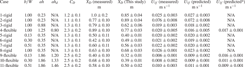
 $X_{D}$ within uncertainty (table 3).
Canopy-averaged velocity,  $U_{1}$, vs distance from the leading edge of a 2-D canopy. Symbols denote measured values. Blue solid curves denote prediction from (2.11)–(2.13) for rigid canopies and (2.24)–(2.28) for flexible canopies. Dashed curves indicate the prediction uncertainty. Horizontal black lines show
 $U_{\infty }$. Vertical dashed lines show the position of predicted
 $X_{D}$. (a) Case 1-rigid,
 $n=520\ \textrm {m}^{-2}$,
 $h=7$ cm,
 $U_{\infty }=6.5\ \textrm {cm}\ \textrm {s}^{-1}$. (b) Case 2-rigid,
 $n=520\ \textrm {m}^{-2}$,
 $h=7$ cm,
 $U_{\infty }=16.5\ \textrm {cm}\ \textrm {s}^{-1}$. (c) Case 3-rigid,
 $n=1370\ \textrm {m}^{-2}$,
 $h=10$ cm,
 $U_{\infty }=6.5\ \textrm {cm}\ \textrm {s}^{-1}$. (d) Case 4-flexible,
 $n=520\ \textrm {m}^{-2}$,
 $h_{d}=9$ cm,
 $U_{\infty }=6.5\ \textrm {cm}\ \textrm {s}^{-1}$.

Measured and predicted  $X_{D}$ and
 $U_{1f}$. Here
 $C_{D}$ was calculated from (3.1) using
 $({U_{\infty }+U_{1f}})/{2}$ as the representative velocity;
 $X_{D}$ (this study) was calculated from (2.11)–(2.13). Uncertainty in
 $X_{D}$ (measured) was half the longitudinal resolution of the velocity measurement. Uncertainty in
 $X_{D}$ (this study) and
 $U_{1f}$ (predicted) propagated from uncertainty in
 $C_{D}$ and
 $K_{c}$. Uncertainty in
 $U_{1f}$ (measured) from spatial variation in measured velocity calculated as the standard error among all time-mean velocity measured in the canopy cross-section (18 points). For flexible meadows, the predicted velocity used the predicted canopy deflection. For comparison, the final column predicts velocity using the measured canopy deflection.

4.2. Rigid 3-D canopies
The velocity predicted for rigid 3-D canopies (blue curves in figure 9) agreed within uncertainty with the measured values (symbols in figure 9), validating the prediction. Note that, although the 3-D analytical solution is strictly valid only for  ${b}/{W}$ and
 ${h}/{H}\ll 1$, the model produced good prediction for
 ${b}/{W}$ as large as 0.51 and
 ${h}/{H}$ as large as 0.34. For reference, the 2-D prediction is included in figure 9 (brown curves). As the canopy became narrower, the 3-D solution deviated more strongly from the 2-D solution. For case 8 (figure 9d), the canopy width was the same as the channel width (
 $b = 1$), and the 3-D solution overlapped with the 2-D solution.
Velocity in 3-D rigid canopies,  $U_{1,3D}$, vs distance from the leading edge. Symbols are measured values. Blue lines denote the 3-D analytical solution (A3)–(A5). Brown lines denote the 2-D solution (2.11)–(2.13). Dashed lines show uncertainty in prediction, based in uncertainty in
 $C_{D}$ and
 $K_{c}$. Horizontal black lines show
 $U_{\infty }$. Vertical dashed lines show
 $X_{D}$ predicted by our analytical model. (a) Case 5,
 $n=775\ \textrm {m}^{-2}$,
 $h=7$ cm,
 ${b}/{W}=0.13$. (b) Case 6,
 $n=775\ \textrm {m}^{-2}$,
 $h=7$ cm,
 ${b}/{W}=0.30$. (c) Case 7,
 $n=775\ \textrm {m}^{-2}$,
 $h=7$ cm,
 ${b}/{W}=0.51$. (d) Case 8,
 $n=775\ \textrm {m}^{-2}$,
 $h=7$ cm,
 ${b}/{W}=1$.

4.3. Flexible 3-D canopies
Flexible canopies bend in response to flow, and the degree of deflection depends on the local velocity. Consistent with this, the measured deflected height was smallest at the leading edge, where the velocity was greatest (symbols, figure 10). The deflected height was predicted from the predicted canopy velocity  $U_{1,3D}$ (from (2.29)) and (2.26) at 0.1 cm intervals from the leading edge, and shown as a smooth curve in figure 10. For the widest canopy (
 ${b}/{W} = 0.5$, figure 10c), the prediction matched the measurement within uncertainty. However, the agreement diminished as the canopy narrowed (figure 10a,b), which was likely due to elevated velocity at the sides of the canopy, i.e. elevated relative to the predicted canopy mean, influencing the pronation of individual blades at the canopy edge.
(a–c) Deflected height of flexible 3-D canopy. Squares denote the measured values. Solid lines denote prediction based on (2.24), (2.25), (2.26) and (2.29). Horizontal black lines denote the un-deflected meadow height. (a) Case 9,  ${b}/{W}=0.13$; (b) case 10,
 ${b}/{W}=0.30$; (c) case 11,
 ${b}/{W}=0.51$. (d) Example of canopy image used to measure the deflected height. White vertical bars denote the position of measurement (
 $x= 5$,
 $10$,
 $15$,
 $20$,
 $30$,
 $41$,
 $51$,
 $61$ and
 $71$ cm).

The predicted 3-D canopy velocity was sensitive to the deflected height. When the deflected height ( $h_{d}$) was correctly predicted (e.g. case 11, figure 10c), the predicted velocity agreed with measured values within uncertainty (figure 11c). However, when
 $h_{d}$ was overpredicted (case 9, figure 10a), the canopy-average velocity was also overpredicted (figure 11a). This is because
 $U_{1f}$ increases with increasing submergence ratio,
 ${h_{d}}/{H}$ (e.g. (2.30)). However, when the velocity prediction used the observed deflected height, it agreed with the measurement within uncertainty (table 3). This illustrates the importance of using the correct deflected height when predicting the canopy velocity. Note that, for all predictions, the velocity at the leading edge was assumed to equal the free stream velocity,
 $U_{1} (x=0)=U_{\infty }$. However, previous studies have observed
 $U_{1} (x=0) < U_{\infty }$. For example, Chen et al. (Reference Chen, Jiang and Nepf2013) observed
 ${U_{1} (x=0)}/{U_{\infty }} = 0.7$ to
 $0.9$ for
 $ah = 0.16$ to
 $1.4$. Nevertheless, the velocity predicted by our analytical model had good agreement with the measurements. This is because the deceleration from
 $U_{\infty }$ to
 $U_{1} (x=0)$ occurred over a length scale that was negligible compared with the adjustment length,
 $X_{D}$, making the assumption
 $U_{1} (x=0)=U_{\infty }$ reasonable for
 $ah\leqslant 1.9$.
Evolution of canopy-averaged velocity,  $U_{1,3D}$, with distance from the leading edge of a flexible, 3-D canopy. The plant density is
 $n= 775\ \textrm {plants}\ \textrm {m}^{-2}$, corresponding to
 $4650\ \textrm {blades}\ \textrm {m}^{2}$. Triangles denote measurements. Blue solid lines denote the prediction based on the predicted deflected height (2.24)–(2.26), (2.28). Blue dashed lines denote the uncertainty in predictions, which came from uncertainty in
 $C_{D}$ and
 $K_{c}$. (a) Case 9,
 ${b}/{W} = 0.13$; (b) case 10,
 ${b}/{W} = 0.30$; and (c) case 11,
 ${b}/{W} = 0.51$.

5. Discussion
5.1. Comparison to live canopies
The 3-D velocity prediction was compared with velocity measured within a 15 cm wide canopy of the real seagrass Z. marina in a 75 cm wide channel (figure 12 in Gambi, Nowell & Jumars Reference Gambi, Nowell and Jumars1990). The water depth was  $H=25$ cm, and the full canopy height was
 $h=11.4\pm 2.5$ cm (figure 1 and table 1 in Gambi et al. Reference Gambi, Nowell and Jumars1990). The deflected height was
 $h_{d}=11\pm 2$,
 $11\pm 2$ and
 $8\pm 2$ cm for
 $U_{\infty }=0.05$,
 $0.10$ and
 $0.20\ \textrm {m}\ \textrm {s}^{-1}$, respectively. The shoot density was
 $1000\ \textrm {m}^{-2}$ which, based on the morphological parameters reported in table 1 of Gambi et al. (Reference Gambi, Nowell and Jumars1990), corresponded to
 $ah=0.9\pm 0.3$. The rigidity of Z. marina blades is reported in Fonseca, Koehl & Fourqurean (Reference Fonseca, Koehl and Fourqurean2019),
 $EI\approx 3\times 10^{-7}\ \textrm {N}\ \textrm {m}^{-2}$. The blade thickness (
 $t=0.2$ mm) and blade material (
 $0.7\ \textrm {g}\ \textrm {cm}^{-3}$) were estimated from Abdelrhman (Reference Abdelrhman2007). The drag coefficient was estimated by (3.1), The measured canopy-average velocity was extracted from profiles presented in figure 2 of Gambi et al. (Reference Gambi, Nowell and Jumars1990). The velocity predicted by the 3-D model agreed with the measurements within uncertainty, validating the model for predictions with real vegetation. Also, the predicted deflected heights,
 $h_{d}=11\pm 1$,
 $10\pm 1$ and
 $7\pm 1$ cm, agreed with the observed
 $h_{d}$ within uncertainty. Finally, the predicted
 $X_{D}$ (shown with vertical dashed lines) increased as velocity increased, which was consistent with the decrease in non-dimensional canopy drag,
 $C_{D}ah_{d}$ (see (2.5)).
5.2. Initial adjustment length,  $X_{D}$, for field conditions

For restoration and ecological assessment, it is useful to consider the scale of a vegetation patch relative to the adjustment length. Chen et al. (Reference Chen, Jiang and Nepf2013) showed that the evolution of velocity from the leading edge of a porous array is not a function of array length,  $L$, such that estimates of
 $X_{D}$ based on a long (
 $L\gg X_{D}$) array can be used as a metric for flow development in any array. In aquatic species, pioneer plants often form short patches when they begin to occupy new space away from the parent population (e.g. Fonseca & Koehl Reference Fonseca and Koehl2006). For short patches, and specifically
 $L\leqslant X_{D}$, the velocity varies across the entire patch, and a large fraction of the canopy experiences a high velocity that can be unfavourable to growth. Consistent with this, a review of seagrass restoration found that restoration success was dependent on vegetation scale, with smaller patch scale associated with lower survival (van Katwijk et al. Reference van Katwijk2016). In contrast, if
 $L\gg X_{D}$, most of the canopy experiences the fully developed velocity which, typically, is significantly reduced from the free stream velocity (e.g. figure 12). A prediction of
 $X_{D}$ would provide a quick assessment of the flow conditions expected within a canopy. With this goal in mind, the new analytical models for velocity evolution were used to calculate
 $X_{D}$ over a range field condition, from which a simple prediction of
 $X_{D}$ was developed. The range of typical field conditions was selected from previous studies. From table 3 of Luhar et al. (Reference Luhar, Coutu, Infantes, Fox and Nepf2010) and table 1 of Hansen & Reidenbach (Reference Hansen and Reidenbach2012), many seagrass species have a submergence ratio from 1 to 5. To avoid
 $h \approx H$, for which our model has not be validated, we consider the range
 $1.5\leqslant {H}/{h}\leqslant 5$. For many seagrass
 $\phi = 0.0004$ to
 $0.04$, which makes negligible impact on the prediction, i.e.
 $\phi \approx 0$. Also,
 $ah$ typically ranges from 0.1 to 10. (e.g. Posidonia oceanica: Pergent-Martini, Rico-Raimondino & Pergent Reference Pergent-Martini, Rico-Raimondino and Pergent1994; Marbá et al. Reference Marbá, Duarte, Cebrián, Gallegos, Olesen and Sand-Jensen1996; Fourqurean et al. Reference Fourqurean, Marbà, Duarte, DÍaz-Almela and Ruiz-Halpern2007; Z. marina: Fonseca & Bell Reference Fonseca and Bell1998; Laugier, Rigollet & de Casabianca Reference Laugier, Rigollet and de Casabianca1999; Guidetti et al. Reference Guidetti, Lorenti, Buia and Mazzella2002). For simplicity,
 $X_{D}$ in figures 13 and 14 was calculated with an assumed
 $C_{D}$ value of 1 and assuming a rigid canopy model. However, the extension to flexible canopies is also discussed.
Evolution of canopy-averaged velocity with distance from the leading edge of a Z. marina canopy. Symbols denote measured values estimated from figure 2 in Gambi et al. (Reference Gambi, Nowell and Jumars1990). Blue solid lines denote the prediction based on the predicted deflected height from (2.24)–(2.26), (2.28). Blue dashed lines denote uncertainty in the prediction based on uncertainty in shoot density and  $K_{c}$. Vertical dashed lines show the predicted
 $X_{D}$. Parameters: (a)
 $U_{\infty }=0.05\ \textrm {m}\ \textrm {s}^{-1}$,
 $C_{D}=2.5\pm 0.3$,
 $X_{D}=0.27$ m; (b)
 $U_{\infty }=0.10\ \textrm {m}\ \textrm {s}^{-1}$,
 $C_{D}=2.4\pm 0.2$,
 $X_{D}=0.41$ m; (c)
 $U_{\infty }=0.20\ \textrm {m}\ \textrm {s}^{-1}$,
 $C_{D}=2.1\pm 0.1$,
 $X_{D}=0.49$ m. Here
 $U_{\infty }$ is shown as a horizontal line in each subplot.

(a) Plot of  ${X_{D}}/{h}$ as a function of
 $C_{D}ah$. Red, green and blue lines denote the condition with
 ${H}/{h}=2$,
 $5$ and
 $20$, respectively. (b) Measured
 ${X_{D}}/{h}$ against the value calculated by (5.1). Blue markers denote the measured data from multiple studies. Open circles: this study, case 1, 2 and 3; squares: Chen et al. (Reference Chen, Jiang and Nepf2013); triangles: Zhang et al. (Reference Zhang, Lei, Huai and Nepf2020); solid circle: this study, case 4 (flexible canopy). For the flexible canopy case,
 ${X_{D}}/{h_{d}}$ (measured) was plotted against
 ${X_{D}}/{h_{d}}$ (5.1). Black dashed line denotes the 1 : 1 ratio. (c) Plot of
 ${U_{1f}}/{U_{\infty }}$ as a function of
 $C_{D}ah$ and
 ${H}/{h}$. (d) Measured
 ${U_{1f}}/{U_{\infty }}$ against predicted
 ${U_{1f}}/{U_{\infty }}$ (by (2.1) and (2.30)). Different markers denote data from different studies (same as subplot (b)). Plots (a,c) are full solutions; (b,d) use the fitted equation, (5.1).

(a) Normalized adjustment length,  ${X_{D}}/({{hb}/({h+b}))}$, as a function of
 ${1}/({C_{D}a({hb}/({h+b})))}$. Black, brown, blue, red and cyan lines denote the conditions
 ${b}/{W}=100$ %, 75 %, 50 %, 25 % and 5 %, respectively. The red and cyan lines overlap. (b) Measured
 ${X_{D}}/({{hb}/({h+b})})$ against predicted
 ${X_{D}}/({{hb}/({h+b})})$ (from (5.2)). (c) Plot of
 ${U_{1f,3D}}/{U_{\infty }}$ as a function of
 ${b}/{W}$ and
 $C_{D}ah$. (d) Measured
 ${U_{1f,3D}}/{U_{\infty }}$ against prediction from (2.22). Red markers denote the measured data from this study. Open circles: case 5, 6, 7 and 8 (rigid canopies); closed circles: case 9, 10 and 11 (flexible canopies). Blue markers denote the 2-D-canopy data from this study and several other studies (same as figure 13b,d). Plots (a,c) are full solutions; (b,d) use the fitted equation, (5.2).

5.2.1. Two-dimensional canopies
A 2-D canopy model will be applicable in the field when the canopy occupies the full width of a channel. The full solution ((2.10) to (2.13)) was run for three different submergence ratios ( ${h}/{H}$), and these solutions provided the values of
 $X_{D}$ and
 $U_{1f}$ plotted in figure 13(a,c). For 2-D canopies, the adjustment length,
 $X_{D}$, depended strongly on the dimensionless canopy density,
 $ah$, but only weakly on the submergence ratio,
 ${H}/{h}$ (figure 13a). The scaling of
 $X_{D}$ in (2.14) shows that
 ${X_{D}}/{h}$ can be described as a function of
 $C_{D}ah$ and
 $(({H-h})/{H})^{2}$. A linear fit between these variables and the adjustment distances predicted from the full model resulted in the following simplified prediction:
 \begin{equation} \left.\begin{gathered} \dfrac{X_{D}}{h} = 3.4+2.5\dfrac{1}{C_{D}ah}-3.3\left(\dfrac{H-h}{H}\right)^{2}.\\ pressure\quad drag\qquad\quad shear \end{gathered}\right\} \end{equation}
The three terms on the right-hand side of (5.1) represent pressure, drag and shear, respectively. For small  $C_{D} ah$, the drag term dominates, and (5.1) has the same form as Chen's prediction (2.5). This illustrates the applicability of the simpler scaling model proposed by Chen, and highlights how the modelling in this paper revealed the more complex dependencies for
 $X_{D}$ on submergence depth. As
 ${H}/{h}$ increases, shear decreases, and the shear term in (2.14) becomes smaller, which results in a shorter
 $X_{D}$ (see figure 13a).
For flexible 2-D canopies, the canopy height is smaller than  $h$. The deflected height,
 $h_{d}$, should be used in (5.1) as a replacement for the geometric height,
 $h$, to normalize
 $X_{D}$ and in the shear term in (5.1). Also, for flexible canopies, the drag scales with
 $C_{D}al_{e}$, and this should be used in place of
 $C_{D}ah$ in the drag term in (5.1). As shown in figure 10, the canopy deflection is the greatest at the leading edge and diminishes along the canopy. Considering that the change in flow velocity is most significant at the leading edge, we anticipate that the deflected height (
 $h_{d0}$) and the effective length (
 $l_{e0}$) at the leading edge should be used in (5.1). With our analytical model,
 $h_{d0}$ and
 $l_{e0}$ can be predicted using (2.24)–(2.27) with
 $U = U_{\infty }$.
As shown in figure 13(b), (5.1) produced good agreement with measured values from this study and several previous studies, including the flexible canopy (solid circle). Figure 13(c) shows  ${U_{1f}}/{U_{\infty }}$ as a function of
 $C_{D} ah$ and
 ${H}/{h}$. Figure 13(d) shows good agreement between the measured
 ${U_{1f}}/{U_{\infty }}$ and the predicted
 ${U_{1f}}/{U_{\infty }}$ (by (2.1) and (2.30)) for both rigid and flexible canopies. For the flexible canopy, (2.30) was applied in an iterative fashion to calculate
 $U_{1f}$. By combining (2.1) and (5.1), one can quickly have an estimation of
 ${X_{D}}/{h}$ and
 ${U_{1f}}/{U_{\infty }}$ to obtain a description of velocity throughout the canopy (figure 13a,c).
5.2.2. Three-dimensional canopies
Drawing on the previously discussed analogy between depth and hydraulic radius, for the 3-D canopies, the reference canopy height,  $h$, was replaced by
 ${hb}/({h+b})$, and the shear term was replaced by
 $(({WH-bh})/{WH})^{2}$. In figure 14(a)
 ${X_{D}}/({{hb}/({h+b})})$, calculated by the full solution given by (A3)–(A5), is plotted as a function of
 ${1}/({C_{D}a(hb/(h+b)))}$ for five width ratios (
 ${b}/{W}$), ranging from 100 % to 5 %. The normalized adjustment length,
 ${X_{D}}/({{hb}/({h+b})})$, decreased as
 ${b}/{W}$ decreased from 100 % (black line). Note that normalizing
 $X_{D}$ by
 ${hb}/({h+b})$ collapses the curves to within a maximum variation of 30 %. However, when
 $X_{D}$ is normalized by
 $h$, the curves for different
 ${b}/{W}$ do not collapse. This supports our statement that, for 3-D canopies,
 $X_{D}$ scales with
 ${hb}/({h+b})$. Hence, for 3-D canopies, we anticipated that (5.1) could be adapted to
 \begin{equation} \frac{X_{D}}{\dfrac{hb}{h+b}} = 3.4+2.5\frac{1}{C_{D}ah\dfrac{b}{h+b}}-3.3\left(\dfrac{WH-bh}{WH}\right)^{2} . \end{equation}
As discussed in § 5.2.1, for flexible canopies, the canopy height in (5.2) is replaced by the deflected canopy height estimated for the leading edge,  $h_{d0}$, and in the canopy drag term
 $C_{D}ah$ is replaced with
 $C_{D}al_{e0}$, with
 $h_{d0}$ and
 $l_{e0}$ estimated from (2.26) and (2.27), using the upstream velocity.
Figure 14(b) compares the prediction from (5.2) and the measured values. The 2-D canopy data were also included in this subplot. Note that the 2-D canopy is equivalent to  $b\rightarrow \infty$, such that
 ${X_{D}}/({{hb}/({h+b}))}={X_{D}}/{h}$. Overall, for both rigid (open markers) and flexible canopies (solid markers), (5.2) produced good agreement with the measurements with a mean deviation of 21 %. Figure 14(c) shows the normalized fully developed velocity (
 ${U_{1f,3D}}/{U_{\infty }}$) predicted from the full solution (A3)–(A5) as a function of the width ratio,
 ${b}/{W}$. A non-monotonic relation between
 ${b}/{W}$ and
 ${U_{1f,3D}}/{U_{\infty }}$ was observed. Specifically, as
 ${b}/{W}$ decreases from 100 % to 10 %,
 ${U_{1f,3D}}/{U_{\infty }}$ decreases as
 ${b}/{W}$ decreases; however, when
 ${b}/{W}$ decreases further,
 ${U_{1f,3D}}/{U_{\infty }}$ increases. This is consistent with (2.21), which shows that as
 ${b}/{W}$ decreases to zero,
 ${U_{1f,3D}}/{U_{\infty }}$ will eventually approach 1. Figure 14(d) shows the comparison between the measured
 ${U_{1f}}/{U_{\infty }}$ against the predicted
 ${U_{1f}}/{U_{\infty }}$ (by (2.1), (2.21), (2.30), (2.31)) for both 3-D and 2-D canopies. For the flexible canopy, (2.30) and (2.31) were applied in an iterative fashion to calculate
 $U_{1f}$ and
 $U_{1f,3D}$, respectively. This further shows that our analytical solution can produce a good prediction of the fully developed velocity.
5.3. Extension to an unbounded domain
The normalized adjustment length,  ${X_{D}}/{h}$, predicted from (A3)–(A5) as a function of the canopy width to height ratio,
 ${b}/{h}$, and canopy drag,
 $C_{D}ah$, in an unbounded domain (
 $W\gg b$) is plotted in figure 15(a), which shows that
 ${X_{D}}/{h}$ increases as
 ${b}/{h}$ increases. Also, (2.32) was used to calculate
 ${U_{1f,3D}}/{U_{\infty }}$ in an unbounded domain. The dependence of
 ${U_{1f,3D}}/{U_{\infty }}$ on
 ${b}/{h}$ and
 $C_{D} ah$ is shown in figure 15(b). In an unbounded domain the within-canopy velocity increases as the patch narrows (decreasing
 ${b}/{h}$). When
 ${b}/{h}<1$, a significant increase in
 ${U_{1f,3D}}/{U_{\infty }}$ occurs. However, when
 ${b}/{h}>2$, a further increase in
 ${b}/{h}$ does not change
 ${U_{1f,3D}}/{U_{\infty }}$. At this point the canopy has reached the unbounded domain limit described by (2.33).
(a) Plot of  ${X_{D}}/{h}$ as a function of
 ${b}/{h}$ and
 $C_{D}ah$ for
 $W\gg b$. In this figure we set
 $h$ and
 $W$ constant, and
 ${b}/{h}$ ranges from 0.1 to 10. Here
 $C_{D} ah=0.5$,
 $1.0$,
 $2.0$ and
 $5.0$, representing typical SAV species;
 ${H}/{h}$ is assumed to be equal to 3, the mean value for typical SAV species. (b) Plot of
 ${U_{1f,3D}}/{U_{\infty }}$ as a function of
 ${b}/{h}$ and
 $C_{D}ah$ for
 $W\gg b$.

6. Conclusion
An analytical model was developed to predict the velocity evolution within a submerged canopy of infinite (2-D) and finite (3-D) width consisting of rigid or flexible canopy elements. The model was validated with laboratory experiments using canopies consisting of rigid cylinders and individual model seagrass plants. As the canopy narrowed, the velocity adjusted more rapidly at the leading edge and reached a lower fully developed velocity. Specifically, the within-canopy velocity  $U_{1}$ was lower, and the adjustment length
 $X_{D}$ was shorter. The adjustment length
 $X_{D}$ also increases as the dimensionless canopy density,
 $ah$, or the submergence ratio,
 ${H}/{h}$, decreases. The analytical solution was used to generate a simplified prediction of
 $X_{D}$ for both 2-D and 3-D canopies. Coupled with the fully developed in-canopy velocity, this provides a way to rapidly assess the flow conditions within a submerged seagrass meadow or array. It should be noted that since the analytical model assumes a spatially uniform velocity outside the canopy, the accuracy of the analytical model will diminish if the edges of the canopy are close to one of the lateral boundaries while not extending up to the boundaries. In that case, the flow velocity on the top of the canopy might be significantly different from that in regions next to the lateral interfaces.
Acknowledgements
This study was supported by Shell International Exploration and Production through the MIT Energy Initiative.
Declaration of interests
The authors report no conflict of interest.
Appendix A
A.1. Simplified expression of the analytical solution to the two-layer model for 2-D meadows when $\phi \ll 1$

When the solid volume fraction is small, i.e.  $\phi \ll 1$, (2.11) can be simplified as follows. Note that
 $\phi \ll 1$ can be applied to various seagrass species. As summarized in Hansen & Reidenbach (Reference Hansen and Reidenbach2012) and Luhar et al. (Reference Luhar, Coutu, Infantes, Fox and Nepf2010), for real seagrass meadows, typically,
 $\phi$ ranges from 0.0004 to 0.04. The parameters in (2.11) can be simplified as
 \begin{equation} \left\{\begin{array}{@{}l} \alpha = \dfrac{[H^{2}-2Hh]h}{(H-h)^{2}}, \\ \beta = C_{2Dim}\left(\dfrac{H}{H-h}\right)^{3}-\dfrac{C_{D}ah}{2}, \\ A' = \dfrac{Hh}{H^{2}-2Hh}U_{\infty}, \\ B' = \dfrac{-2}{1 - \dfrac{C_{D}ah}{2C}\left(\dfrac{H-h}{H}\right)^{3}}U_{\infty}, \\ C' = \dfrac{1}{1 - \dfrac{C_{D}ah}{2C}\left(\dfrac{H-h}{H}\right)^{3}}U_{\infty}^{2}. \end{array} \right. \end{equation}
A.2. Complete solution to the two-layer model for 3-D meadows
Equation (2.20) is repeated here for completeness of the solution, i.e.
 \begin{align} &\frac{\textrm{d} U_{1,3D}(x)}{\textrm{d} x}bh\frac{U_{1,3D}(x)[(WH-bh)^{2}-(1-\phi)^{2}(bh)^{2}]+U_{\infty}WHbh(1-\phi)}{(WH-bh)^{3}} \nonumber\\ &\quad = C_{3Dim}(b+h)\left[U_{\infty}-U_{1,3D}(x)\left(1-\frac{bh}{WH}\phi\right)\right]^{2} \left(\frac{WH}{WH-bh}\right)^{3} \nonumber\\ &\qquad - \frac{C_{D}abh}{2(1-\phi)}U_{1,3D}(x)^{2}. \end{align}
 \begin{equation} \left\{\begin{array}{@{}l}
\alpha_{3D} = \dfrac{[(WH-bh)^{2} -
(1-\phi)^{2}(bh)^{2}]bh}{(WH-bh)^{2}}, \\
\beta_{3D} =
C_{3Dim}(b+h)\left(\dfrac{WH}{WH-bh}\right)^{3}
\left(1-\dfrac{bh}{WH}\phi\right)^{2}-\dfrac{C_{D}abh}{2(1-\phi)},
\\ A'_{3D} = \dfrac{WHbh(1-\phi)}{(WH-bh)^{2} -
(1-\phi)^{2}(bh)^{2}}U_{\infty}, \\ B'_{3D} =
\dfrac{-2\left(1-\dfrac{bh}{WH}\phi\right)}{\left(1-\dfrac{bh}{WH}\phi\right)^{2}
-
\dfrac{C_{D}abh}{2C_{3Dim}(b+h)(1-\phi)}\left(\dfrac{WH-bh}{WH}\right)^{3}}U_{\infty},
\\ C'_{3D} =
\dfrac{1}{\left(1-\dfrac{bh}{WH}\phi\right)^{2} -
\dfrac{C_{D}abh}{2C_{3Dim}(b+h)(1-\phi)}\left(\dfrac{WH-bh}{WH}\right)^{3}}U_{\infty}^{2},
\end{array} \right. \end{equation}
and substitute (A3) into (A2), we get
 \begin{equation} \frac{\alpha_{3D}}{\beta_{3D}}\frac{U_{1,3D}(x)+A'_{3D}}{U_{1,3D}(x)^{2}+B'_{3D}U_{1,3D}(x)+C'_{3D}}\,\textrm{d} U_{1,3D}(x) = {\textrm{d} x} . \end{equation}
Integrating (A4) yields
 \begin{equation} \left\{\begin{array}{@{}l} f(U) = \displaystyle\int\dfrac{U+A'_{3D}}{U^{2}+B'_{3D}U+C'_{3D}}\,\textrm{d}U = \dfrac{2A'_{3D}-B'_{3D}}{\sqrt{4C'_{3D}-B'^{2}_{3D}}}\arctan{\dfrac{B'_{3D}+2U_{3D}}{\sqrt{4C'_{3D}-B'^{2}_{3D}}}} \\ \qquad\quad+\dfrac{1}{2}\ln{(U^{2}+B'_{3D}U+C'_{3D})}, \\ f(U_{1,3D}(x)) - f(U_{\infty}) = \dfrac{\beta_{3D}}{\alpha_{3D}}x. \end{array} \right. \end{equation}
A.3. A detailed description of how we computed the flow development
The modelled flow developed was computed by a MATLAB program based on (2.26)–(2.29). The procedures are listed as follows.
(1) At
$x=0$, use the initial conditions $U_{1}(x_{i=0})=U_{\infty }$. The flow development was computed with 0.002 m ($\Delta x$) intervals.(2) Use (2.22) to calculate the Cauchy number with
$U_{1}(x_{i})$.(3) Use (2.26) and (2.27) to calculate the deflected height and the effective length.
(4) Use (2.28) and (2.29) to calculate
${\textrm {d}U_{1}(x_{i})}/{\textrm {d} x}$.(5) Forward Euler's method was used to calculate
$U_{1}(x_{i+1})$. Specifically, $U_{1}(x_{i+1}) = ({\textrm {d}U_{i}(x_{i})}/{\textrm {d} x})\Delta x + U_{1}(x_{i})$.(6) Repeat steps (2)–(5).