



1 Introduction
We say that a real-valued function f on
 $\mathbb {R}^n$
is in the non-homogeneous Hölder class of order
 $s,$
with
 $0 < s < 1,$
denoted
 $f \in \Lambda _{s}(\mathbb {R}^n)$
or just
 $f \in \Lambda _{s}$
when there is no ambiguity, if it is uniformly bounded and
 $$ \begin{align} \sup_{x,\, 0 < |y| < 1} \frac{|f(x+y)-f(x)|}{|y|^s} + \left\lVert f \right\rVert_{\mathrm{L}^{\infty}(\mathbb{R}^n)} < \infty, \end{align} $$
where
 $|x|$
stands for the euclidean norm of
 $x \in \mathbb {R}^n.$
In order to define all smoothness classes
 $s> 0$
, we first note that in the range
 $s \in (0,2)$
, the norm in
 $\Lambda _{s}$
may be defined by using second differences:
 $$ \begin{align} \left\lVert f \right\rVert_{\Lambda_{s}} := \sup_{x,\, 0 < |y| < 1} \frac{|f(x+y) -2f(x) + f(x-y)|}{|y|^s} + \left\lVert f \right\rVert_{\mathrm{L}^{\infty}(\mathbb{R}^n)}, \end{align} $$
and the norms (1) and (2) are equivalent for
 $s \in (0,1).$
In general, if
 $s> 0$
and
 $s = m + t,$
with
 $m \in \mathbb {N}_0$
and
 $0 < t \leq 1,$
we define the Hölder class
 $\Lambda _{s}$
as the space of bounded functions that are m times continuously differentiable with all their derivatives of order m belonging to
 $\Lambda _{t}.$
The norm of
 $f \in \Lambda _{s}$
may be defined as
 $\left \lVert f \right \rVert _{\Lambda _{s}} := \sup _{|\alpha | = m} \left \lVert \partial ^\alpha f \right \rVert _{\Lambda _{t}} + \left \lVert f \right \rVert _{\mathrm {L}^{\infty }}(\mathbb {R}^n),$
which is equivalent to (2) for
 $s \in (0,2).$
In the case
 $s = 1$
, we obtain the so-called non-homogeneous Zygmund class. This space is often denoted by
 $\Lambda _{\ast }(\mathbb {R}^n)$
or just
 $\Lambda _{\ast }$
—thus as Banach spaces
 $\Lambda _{\ast }(\mathbb {R}^n) = \Lambda _{1}(\mathbb {R}^n)$
—and we denote the corresponding seminorm by
 $$ \begin{align} \left\lVert f \right\rVert_{\dot{\Lambda}_{\ast}} := \sup_{x,\, 0 < |y| < 1} \frac{|f(x+y) - 2f(x) + f(x-y)|}{|y|}. \end{align} $$
If f is a polynomial of degree at most
 $1,$
then we have that
 $\left \lVert f \right \rVert _{\dot {\Lambda }_{\ast }} = 0.$
Note that the norm in
 $\Lambda _{\ast }$
is given by
 $\left \lVert f \right \rVert _{\Lambda _{\ast }} = \left \lVert f \right \rVert _{\dot {\Lambda }_{\ast }} + \left \lVert f \right \rVert _{\mathrm {L}^{\infty }}.$
The Zygmund class is the natural definition of the Hölder classes
 $\Lambda _{s}$
for
 $s = 1$
as is suggested by (2), and this definition is more properly validated by the coincidence
 $\Lambda _{s} = \mathrm {B}^{s}_{{\infty },{\infty }}$
for all
 $s> 0,$
where
 $\mathrm {B}^{s}_{{p},{q}}$
stands for the classical Besov space. The classes
 $\Lambda _{s}$
have numerous applications, e.g., to PDE’s and polynomial approximation or Calderón–Zygmund theory, and have been extensively studied (see, for instance, [Reference Donaire, Llorente and NicolauDLN14, Reference MakarovMak89], [Reference SteinSte71, Chapter V], [Reference TriebelTri10, Reference ZygmundZyg45]).
From now on, we will restrict ourselves to the spaces
 $\Lambda _{s}$
for
 $0 < s \leq 1,$
although we could also formulate our results for all
 $s> 0,$
but this would not bring anything essentially new apart from some additional non-interesting technicalities.
A locally integrable function f on
 $\mathbb {R}^n$
is said to have bounded mean oscillation,
 $f \in \mathrm {BMO}(\mathbb {R}^n)$
or just
 $f \in \mathrm {BMO},$
if
 $$ \begin{align*} \left\lVert f \right\rVert_{\mathrm{BMO}} := \sup_Q \left(\frac{1}{|Q|} \int_Q |f(x)-f_Q|^2 \, dx\right)^{1/2} < \infty, \end{align*} $$
where Q ranges over all finite cubes with sides parallel to the axes in
 $\mathbb {R}^n$
and where
 $$ \begin{align*} f_Q := \frac{1}{|Q|} \int_Q f(x)\, dx \end{align*} $$
is the average of f on
 $Q.$
We refer to [Reference SteinSte93] for basic facts on the space
 $\mathrm {BMO}.$
Actually, as we will, in general, deal with non-homogeneous spaces, we are more interested in the non-homogeneous
 $\mathrm {BMO}$
space, denoted by
 $\mathbf {bmo}(\mathbb {R}^n)$
following Triebel’s convention. To be precise, consider the collection
 $\mathcal {D}_0$
of dyadic cubes in
 $\mathbb {R}^n$
of side-length 1, that is, the set of cubes Q of the form
 $$ \begin{align*} Q = \{x \in \mathbb{R}^n\colon x-k \in [0,1]^n\} \end{align*} $$
for some
 $k \in \mathbb {Z}^n$
. The Banach space
 $\mathbf {bmo}(\mathbb {R}^n)$
consists of all functions
 $f \in \mathrm {BMO}(\mathbb {R}^n)$
that are locally uniformly in
 $\mathrm {L}^{2},$
i.e., those functions such that
 $$ \begin{align} \left\lVert f \right\rVert_{\mathbf{bmo}} := \left\lVert f \right\rVert_{\mathrm{BMO}} + \sup_{Q \in \mathcal{D}_0} \left(\int_Q |f(x)|^2\, dx\right)^{1/2} < \infty. \end{align} $$
We also need to define the scale of non-homogeneous
 $\mathbf {bmo}$
-Sobolev spaces. We first fix our convention for the Fourier transform. For a given function
 $f \in \mathrm {L}^{1}(\mathbb {R}^n),$
we define its Fourier transform
 $\mathcal {F}\left [{f}\right ] = \hat {f}$
using the convention
 $$ \begin{align*} \mathcal{F}\left[{f}\right](\xi) := \int_{\mathbb{R}^n} f(x) e^{-i x\cdot\xi}\, dx, \quad \xi \in \mathbb{R}^n. \end{align*} $$
Given
 $r \in \mathbb {R},$
the standard lift operator
 $\mathrm {J}^{r}$
is defined via the Bessel potential: for a Schwartz distribution f, one sets
 $$ \begin{align*} \mathrm{J}^{r} f(x) := \mathcal{F}^{-1}\left[{(1+|\xi|^2)^{-r/2} \mathcal{F}\left[{f}\right](\xi)}\right](x). \end{align*} $$
Due to the lift property of this operator, one has, e.g., for the Hölder spaces, the relation
 $\mathrm {J}^{r} \Lambda _{s}(\mathbb {R}^n) = \Lambda _{s+r}(\mathbb {R}^n)$
for all
 $s,r> 0,$
and this equality may be used to define the space
 $\Lambda _{s}(\mathbb {R}^n)$
also for
 $s \leq 0.$
The Banach space
 $\mathrm {J}_{s}(\mathbf {bmo})(\mathbb {R}^n)$
consists of all functions
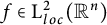 $f \in \mathrm {L}^{2}_{loc}(\mathbb {R}^n)$
such that
 $\mathrm {J}^{-s}f \in \mathbf {bmo}(\mathbb {R}^n),$
and we set
 $$ \begin{align*} \left\lVert f \right\rVert_{\mathrm{J}_{s}(\mathbf{bmo})} := \left\lVert \mathrm{J}^{-s}f \right\rVert_{\mathbf{bmo}}. \end{align*} $$
Here, if one replaces the condition
 $f \in \mathrm {L}^{2}_{loc}$
by
 $f \in \mathcal {S}'$
, the above definition extends to all
 $s \in \mathbb {R}$
. As we will see later on, for each
 $s> 0$
, we have the strict inclusion
 $$ \begin{align*} \mathrm{J}_{s}(\mathbf{bmo}) \subsetneq \Lambda_{s}. \end{align*} $$
In [Reference Nicolau and Soler i GibertNS20], the authors give an estimate in terms of second differences for the distance of a compactly supported function
 $f \in \Lambda _{\ast }$
to the subspace
 $\mathrm {I}_{1}(\mathrm {BMO})(\mathbb {R})$
consisting of continuous functions with distributional derivative in
 $\mathrm {BMO}$
—this space is the homogeneous counterpart of the space
 $\mathrm {J}_{1}(\mathbf {bmo})$
we defined previously. The result in [Reference Nicolau and Soler i GibertNS20] is analogous to that obtained by Ghatage and Zheng in [Reference Ghatage and ZhengGZ93], where they estimate the distance of a function in the Bloch space to the subspace of analytic
 $\mathrm {BMO}$
functions in terms of its hyperbolic derivative. In this connection, we mention also the paper of Garnett and Jones [Reference Garnett and JonesGJ78], where a formula for the distance from
 $\mathrm {BMO}$
to bounded functions is established.
In order to state the result in [Reference Nicolau and Soler i GibertNS20] and our generalization, it is useful to define for a given continuous function f on
 $\mathbb {R}^n$
its (maximal) second difference at point
 $x \in \mathbb {R}^n$
and scale
 $y> 0$
by the quantity
 $$ \begin{align*} \Delta_2f(x,y) := \sup_{|h| = y} |f(x+h) - 2f(x) + f(x-h)|. \end{align*} $$
We will always consider these second differences to be defined on the upper half-space, that is,
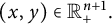 $(x,y) \in \mathbb {R}^{n +1}_+.$
Moreover, if
 $X \subset \Lambda _{s}$
is a subspace of the Hölder class of order
 $s,$
we define the distance of
 $f \in \Lambda _{s}$
to X as
 $$ \begin{align*} \mathrm{dist}_s(f,X) := \inf_{g \in X} \left\lVert f-g \right\rVert_{\Lambda_{s}}. \end{align*} $$
The estimate in [Reference Nicolau and Soler i GibertNS20] is given in terms of a Carleson-type condition on the set where the quantities
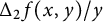 $\Delta _2 f(x,y)/y$
are large, for
 $x \in \mathbb {R}$
and
 $y> 0.$
Namely, for
 $f \in \Lambda _{\ast }(\mathbb {R})$
and
 $\varepsilon> 0$
, consider the set
 $$ \begin{align*} S(f,\varepsilon) := \{(x,y) \in \mathbb{R}^2_+\colon \Delta_2f(x,y)> \varepsilon y\} \end{align*} $$
in the upper half-plane and the quantity
 $$ \begin{align*} M(f,\varepsilon) := \sup_I \frac{1}{|I|} \int_I\int_0^{|I|} \chi_{S(f,\varepsilon)}(x,y)\, \frac{dy\, dx}{y}, \end{align*} $$
where I ranges over all intervals. Recall here that
 $$ \begin{align*} \mathrm{I}_{1}(\mathrm{BMO})(\mathbb{R}) = \{f\in\mathcal{C}(\mathbb{R})\colon f' \in \mathrm{BMO}\}, \end{align*} $$
where the derivative is taken in the distributional sense. Then, the following holds.
Theorem A [Reference Nicolau and Soler i GibertNS20]
Let f be a compactly supported function in
 $\Lambda _{\ast }(\mathbb {R}).$
Then,
 $$ \begin{align*} \mathrm{dist}_1 (f,\mathrm{I}_{1}(\mathrm{BMO})) \simeq \inf \{\varepsilon> 0\colon M(f,\varepsilon) < \infty\}. \end{align*} $$
Some remarks are in order here. First of all, the precise theorem in [Reference Nicolau and Soler i GibertNS20] uses only the homogeneous seminorm
 $\left \lVert \cdot \right \rVert _{\dot {\Lambda }_{\ast }}$
when defining the distance of a function to the subspace in question. However, this makes no real difference, because f is compactly supported. Second, Theorem A involves the homogeneous
 $\mathrm {BMO}$
-Sobolev space, but one may observe that the non-homogeneous norm is equivalent for functions supported on a fixed compact subset.
The proof in [Reference Nicolau and Soler i GibertNS20] makes use of Strichartz’s [Reference StrichartzStr80] characterization of homogeneous
 $\mathrm {BMO}$
-Sobolev spaces in terms of second differences and exhibits a rather intricate transfer from dyadic spaces to the non-dyadic situation. This method appears to be restricted to dimension
 $n = 1.$
In this paper, our goal is to generalize Theorem A in two directions: first of all, we will treat functions on
 $\mathbb {R}^n$
for arbitrary
 $n \geq 1$
and, second, we consider not just the Zygmund class but functions in all classes
 $\Lambda _{s}(\mathbb {R}^n)$
for
 $0 < s \leq 1.$
As a by-product, we provide a new approach to Theorem A.
We now turn to precise formulation of the results of the present paper. Some of them will be expressed in terms of a Carleson-type measure for the size of subsets of the upper half-space, analogously to Theorem A, and it is useful to have a general definition for this purpose. Consider the set
 $\mathcal {D}$
of dyadic cubes of side-length at most one in
 $\mathbb {R}^n,$
that is, the set of cubes of the form
 $$ \begin{align*} Q = \{x \in \mathbb{R}^n\colon 2^jx-k \in [0,1]^n\}, \quad j \in \mathbb{N}_0, k \in \mathbb{Z}^n. \end{align*} $$
For a given measurable subset
 $A \subseteq \mathbb {R}^{n +1}_+,$
we define the quantity
 $M(A)$
by
 $$ \begin{align} M(A) := \sup_{Q \in \mathcal{D}} \frac{1}{|Q|} \int_Q\int_0^{l(Q)} \chi_A(x,y)\, \frac{dy\, dx}{y}. \end{align} $$
Note that the finiteness of
 $M(A)$
is equivalent to
 $y^{-1} \chi _A(x,y)\, dx\, dy$
being a Carleson measure in the upper half-space (see [Reference SteinSte93, Section II.2]).
Toward our first characterization, given a function
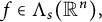 $f \in \Lambda _{s}(\mathbb {R}^n),$
with
 $0 < s \leq 1,$
consider the set
 $$ \begin{align*} S(s,f,\varepsilon) := \{(x,y) \in \mathbb{R}^{n +1}_+\colon \Delta_2f(x,y)> \varepsilon y^s\}. \end{align*} $$
This should be thought as the set of points
 $(x,y)$
in the upper half-space for which its associated second difference is large with respect to the corresponding scale. The following result generalizes Theorem A for arbitrary dimension
 $n \geq 1$
and smoothness in the range
 $0 < s \leq 1.$
Theorem 1 Let
 $0 < s \leq 1$
, and consider a function
 $f \in \Lambda _{s}(\mathbb {R}^n)$
. Then,
 $$ \begin{align} \mathrm{dist}_s (f,\mathrm{J}_{s}(\mathbf{bmo})) \simeq \inf \{\varepsilon> 0\colon M(S(s,f,\varepsilon)) < \infty\}. \end{align} $$
A main tool for us will be the wavelet characterization of the function spaces involved. For that end, we next recall the basic properties of wavelets. Consider the space
 $\mathrm {L}^{2}(\mathbb {R}^n)$
of square integrable functions on
 $\mathbb {R}^n.$
It is known that, for any
 $r \in \mathbb {N}_0,$
there exist compactly supported real-valued functions
 $$ \begin{align*} \varphi \in \mathcal{C}_0^r(\mathbb{R}^n) \quad \text{and} \quad \psi_l \in \mathcal{C}_0^r(\mathbb{R}^n), \quad \text{with } 1 \leq l \leq 2^n-1, \end{align*} $$
such that their dyadic translations and dilations form an orthonormal basis of
 $\mathrm {L}^{2}(\mathbb {R}^n).$
To be more precise, the set
 $$ \begin{align*} \{\varphi(x-k)\colon k \in \mathbb{Z}^n\} \cup \{2^{jn/2} \psi_l(2^jx-k)\colon 1 \leq l \leq 2^n-1, j \in \mathbb{N}_0, k \in \mathbb{Z}^n\} \end{align*} $$
forms an orthonormal basis of
 $\mathrm {L}^{2}(\mathbb {R}^n).$
Moreover, we additionally have that
 $$ \begin{align*} \int_{\mathbb{R}^n} x^\alpha \psi_l(x)\, dx = 0 \end{align*} $$
for any multi-index
 $\alpha \in \mathbb {N}_0^n$
such that
 $|\alpha | \leq r$
and for every
 $1 \leq l \leq 2^n-1.$
Such a set of functions is called a wavelet basis of regularity
 $r.$
For a detailed explanation on how to construct such bases, see, for instance, [Reference MeyerMey92].
It will be useful to index the wavelets in terms of dyadic cubes. Thus, recall that we denote by
 $\mathcal {D}$
the set of dyadic cubes on
 $\mathbb {R}^n$
of side-length at most one, and, for
 $j \in \mathbb {N}_0,$
let us denote the set of cubes
 $Q \in \mathcal {D}$
of side-length
 $l(Q) = 2^{-j}$
by
 $\mathcal {D}_j.$
Assuming that
 $Q \in \mathcal {D}_j,$
we let
 $\tau (Q) := j$
denote the dyadic level of
 $Q.$
Given
 $k \in \mathbb {Z}^n,$
let
 $Q = \{x \in \mathbb {R}^n\colon x-k \in [0,1]^n\} \in \mathcal {D}_0$
and denote
 $$ \begin{align*} \varphi_Q(x) = \varphi(x-k). \end{align*} $$
Analogously, given
 $j \in \mathbb {N}_0$
and
 $k \in \mathbb {Z}^n,$
let
 $Q = \{x \in \mathbb {R}^n\colon 2^jx-k \in [0,1]^n\} \in \mathcal {D}_j$
and write
 $$ \begin{align*} \psi_{(l,Q)}(x) = 2^{jn/2} \psi_l(2^jx-k) \end{align*} $$
for
 $1 \leq l \leq 2^n-1.$
For future convenience, we define
 $\mathcal {Q} = \{(l,Q)\colon 1 \leq l \leq 2^n-1, Q \in \mathcal {D}\}$
, and, for
 $\omega = (l,Q) \in \mathcal {Q},$
we denote
 $|\omega | := \tau (Q).$
In addition, we use the notation
 $\mathcal {Q}_j = \{\omega \in \mathcal {Q}\colon |\omega | = j\}$
for
 $j \in \mathbb {N}_0.$
Finally, if
 $Q \in \mathcal {D},$
then we denote by
 $\mathcal {Q}(Q)$
the set of
 $(l,P) \in \mathcal {Q}$
for which
 $P \subseteq Q.$
Consider a wavelet basis
 $\{\varphi _Q\colon Q \in \mathcal {D}_0\} \cup \{\psi _\omega \colon \omega \in \mathcal {Q}\}$
of regularity
 $r.$
Let f be a function in
 $\Lambda _{s}$
for some
 $0 < s \leq 1.$
The wavelet coefficients of f are
 $$ \begin{align*} d_Q(f) = \int_{\mathbb{R}^n} f(x) \overline{\varphi_Q(x)}\, dx, \quad Q \in \mathcal{D}_0, \end{align*} $$
and
 $$ \begin{align*} c_{(l,Q)}(f) = c_\omega(f) := \int_{\mathbb{R}^n} f(x)\overline{\psi_\omega(x)}\, dx, \quad (l,Q) = \omega \in \mathcal{Q}. \end{align*} $$
From now on, because we only consider real-valued wavelets, we might omit the complex conjugation in the definition of the wavelet coefficients. In addition, these coefficients can actually be defined for a much wider class of distributions, but we will not require this level of generality. In [Reference Lemarié and MeyerLM86], Lemarié and Meyer characterize when a wavelet series f is in the space
 $\Lambda _{s},$
for
 $s> 0,$
in terms of its wavelet coefficients
 $\{d_Q(f)\}$
and
 $\{c_\omega (f)\}.$
See also [Reference Aimar and BernardisAB97] and [Reference MeyerMey92, Section 6.4] for a more detailed explanation.
Theorem B (Lemarié and Meyer)
Let
 $s> 0$
, and consider a wavelet basis
 $\{\varphi _Q\colon Q \in \mathcal {D}_0\} \cup \{\psi _\omega \colon \omega \in \mathcal {Q}\}$
of regularity
 $r> s$
. The wavelet series
 $$ \begin{align*} f(x) = \sum_{Q \in \mathcal{D}_0} d_Q(f) \varphi_Q(x) + \sum_{\omega\in\mathcal{Q}} c_\omega(f) \psi_\omega(x), \quad x\in\mathbb{R}^n, \end{align*} $$
is in
 $\Lambda _{s}(\mathbb {R}^n)$
if and only if
 $$ \begin{align} \sup_{Q \in \mathcal{D}_0} |d_Q(f)| + \sup_{\omega \in \mathcal{Q}} 2^{|\omega|(n/2+s)}|c_\omega(f)| < \infty. \end{align} $$
Moreover, if
 $\left \lVert \{d(f),c(f)\} \right \rVert _{s}$
is the left-hand side in (7), then
 $\left \lVert \{d(f),c(f)\} \right \rVert _{s} \simeq \left \lVert f \right \rVert _{\Lambda _{s}}.$
In [Reference Lemarié and MeyerLM86], the authors also give a wavelet characterization for functions in the space
 $\mathrm {BMO}$
(see also [Reference Aimar and BernardisAB97], [Reference MeyerMey92, Section 5.6], [Reference SteinSte93, Section IV.4.5] for detailed expositions on the topic). However, we need the following wavelet characterization for the non-homogeneous
 $\mathbf {bmo}$
-Sobolev spaces. To the best of our knowledge, such a characterization using smooth wavelets appears first as a particular case of a theorem of Frazier and Jawerth in [Reference Frazier and JawerthFJ90].
Theorem 2 Let
 $s> 0$
, and consider a wavelet basis
 $\{\varphi _Q\colon Q \in \mathcal {D}_0\} \cup \{\psi _\omega \colon \omega \in \mathcal {Q}\}$
of regularity
 $r> s.$
The wavelet series
 $$ \begin{align*} f(x) = \sum_{Q \in \mathcal{D}_0} d_Q(f) \varphi_Q(x) + \sum_{\omega \in \mathcal{Q}} c_\omega(f) \psi_\omega(x), \quad x\in\mathbb{R}^n, \end{align*} $$
represents an element in
 $\mathrm {J}_{s}(\mathbf {bmo})(\mathbb {R}^n)$
if and only if
 $$ \begin{align} \sup_{Q \in \mathcal{D}_0} |d_Q(f)| + \sup_{Q \in \mathcal{D}} \left(\frac{1}{|Q|} \sum_{\omega \in \mathcal{Q}(Q)} 4^{|\omega|s}|c_\omega(f)|^2\right)^{1/2} < \infty. \end{align} $$
Moreover, the above quantity is comparable to
 $\left \lVert f \right \rVert _{\mathrm {J}_{s}(\mathbf {bmo})}.$
It turns out that the characterization of the distance to
 $\mathrm {J}_{s}(\mathbf {bmo})$
can be done in a rather simple way with the above notation in terms of wavelet coefficients. In particular, we make use of the unconditional convergence of the wavelet series appearing in Theorems B and 2, both in the spaces
 $\Lambda _{s}(\mathbb {R}^n)$
and in the spaces
 $\mathrm {J}_{s}(\mathbf {bmo})(\mathbb {R}^n)$
(of course, this convergence must be understood not in norm, but in the sense of distributions). Let
 $0 < s \leq 1$
,
 $\varepsilon> 0$
, and fix a wavelet basis
 $\{\varphi _Q\colon Q \in \mathcal {D}_0\} \cup \{\psi _\omega \colon \omega \in \mathcal {Q}\}$
. Given a function
 $f \in \Lambda _{s}(\mathbb {R}^n)$
with wavelet coefficients
 $\{c_\omega (f)\}$
, we consider the set
 $$ \begin{align*} W(s,f,\varepsilon) := \bigcup_{j \in \mathbb{N}_0} \{Q \in \mathcal{D}_j\colon \sup_l |c_{(l,Q)}(f)|> \varepsilon 2^{-j(n/2+s)}\} \end{align*} $$
and the associated set
 $T(s,f,\varepsilon ) \subseteq \mathbb {R}^{n +1}_+$
defined by
 $$ \begin{align*} T(s,f,\varepsilon) := \bigcup_{Q \in W(s,f,\varepsilon)} T(Q), \end{align*} $$
where for a given cube
 $Q \in \mathcal {D}$
, we denote
 $T(Q) = \{(x,y) \in \mathbb {R}^{n +1}_+\colon x \in Q, l(Q)/2 \leq y \leq l(Q)\}.$
Observe that
 $T(s,f,\varepsilon )$
comprises those top half-cubes in
 $\mathbb {R}^{n +1}_+$
corresponding to cubes in
 $\mathcal {D}$
having at least one associated wavelet coefficient
 $c_\omega (f)$
large with respect to its scale. Moreover, we emphasize that the sets
 $W(s,f,\varepsilon )$
and
 $T(s,f,\varepsilon )$
do not take into account the wavelet coefficients
 $\{d_Q(f)\}$
corresponding to function
 $\varphi .$
Theorem 3 Let
 $0 < s \leq 1$
and
 $\varepsilon> 0.$
Consider a wavelet basis
 $\{\varphi _Q\colon Q \in \mathcal {D}_0\} \cup \{\psi _\omega \colon \omega \in \mathcal {Q}\}$
of regularity
 $r> s,$
a function
 $f \in \Lambda _{s}(\mathbb {R}^n)$
, and the corresponding set
 $T(s,f,\varepsilon )$
defined in terms of this wavelet basis. Then, we have that
 $$ \begin{align} \mathrm{dist}_s(f,\mathrm{J}_{s}(\mathbf{bmo})) \simeq \inf \{\varepsilon>0\colon M(T(s,f,\varepsilon)) < \infty\}. \end{align} $$
Note that the infimum in (9) is taken over a non-empty set, because for any function
 $f \in \Lambda _{s}(\mathbb {R}^n)$
with wavelet coefficients
 $\{d_Q(f)\}$
and
 $\{c_\omega (f)\}$
, one has that
 $M(T(s,f,\left \lVert \{d(f),c(f)\} \right \rVert _{s})) = 0,$
where
 $$ \begin{align*} \left\lVert \{d(f),c(f)\} \right\rVert_{s} := \sup_{Q \in \mathcal{D}_0} |d_Q(f)| + \sup_{\omega \in \mathcal{Q}} 2^{|\omega|(n/2+s)}|c_\omega(f)|. \end{align*} $$
Of course, here, the values of the coefficients
 $\{d_Q(f)\}$
do not play any role as long as they are uniformly bounded. This is because in this situation the series
 $\sum _{Q\in \mathcal {D}_0} d_Q(f) \varphi _Q \in \mathrm {J}_{s}(\mathbf {bmo})$
for
 $s < r.$
Therefore, to estimate
 $\mathrm {dist}_s(f,\mathrm {J}_{s}(\mathbf {bmo}))$
, we could assume that
 $d_Q(f) = 0$
for all
 $Q \in \mathcal {D}_0$
without loss of generality. Observe as well that the set
 $T(s,f,\varepsilon )$
might depend on the wavelet basis we choose. Nonetheless, this will have no consequence for our results, because we will focus on the comparability between the infima in equations (6) and (9), and to that end, we will consider a fixed wavelet basis of enough regularity.
Another way to characterize when a continuous bounded function f belongs to
 $\Lambda _{s}(\mathbb {R}^n),$
for
 $0 < s \leq 1,$
is by means of the hyperbolic derivatives of its Poisson extension to the upper half-space. Namely, let us denote by
 $P_y(x)$
the Poisson kernel on the upper half-space
 $\mathbb {R}^{n +1}_+,$
and by u the harmonic extension of
 $f,$
that is,
 $u(x,y) = \mathrm {P}\left [{f}\right ](x,y) = (P_y \ast f)(x).$
Given
 $0 < s \leq 1,$
a continuous function f is in
 $\Lambda _{s}(\mathbb {R}^n)$
if and only if
 $$ \begin{align} \left\lVert f \right\rVert_{\mathrm{L}^{\infty}} + \sup_{(x,y)\in\mathbb{R}^{n +1}_+} y^{2-s} \left|\frac{\partial^2 u}{\partial y^2}(x,y)\right| < \infty. \end{align} $$
Moreover, the above quantity is comparable to
 $\left \lVert f \right \rVert _{\Lambda _{s}}.$
For a detailed exposition on the topic, see [Reference SteinSte71, pp. 141–149]. This motivates us to estimate the distance of a given function
 $f \in \Lambda _{s}(\mathbb {R}^n)$
to the subspace
 $\mathrm {J}_{s}(\mathbf {bmo})(\mathbb {R}^n)$
in terms of these hyperbolic derivatives. Consider the set
 $$ \begin{align*} D(s,f,\varepsilon) = \left\{(x,y) \in \mathbb{R}^{n +1}_+\colon y^2\left|\frac{\partial^2 \mathrm{P}\left[{f}\right]}{\partial y^2}(x,y)\right|> \varepsilon y^s\right\}, \end{align*} $$
that is, the set of points in the upper half-space for which the second hyperbolic derivative of f is large with respect to the corresponding scale. We have the following result.
Theorem 4 Let
 $0 < s \leq 1,$
and consider a function
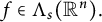 $f \in \Lambda _{s}(\mathbb {R}^n).$
Then,
 $$ \begin{align} \mathrm{dist}_s (f,\mathrm{J}_{s}(\mathbf{bmo})) \simeq \inf \{\varepsilon> 0\colon M(D(s,f,\varepsilon)) < \infty\}. \end{align} $$
Our proof of Theorems 1 and 4 will be via Theorem 3. However, the reduction is rather nontrivial and will be based on careful comparison of the sets
 $S(s,f,\varepsilon )$
,
 $D(s,f,\varepsilon )$
, and
 $T(s,f,\varepsilon )$
. Our aim is to show that there are inequalities of the type
 $M(T(s,f,\varepsilon )) \lesssim M(S(s,f,c\varepsilon ))$
, and similar inequalities between the other pairs, for an absolute constant
 $c> 0$
. The proofs of these inequalities employ suitable inclusions between hyperbolically dilated sets. The inequalities then easily yield Theorems 1 and 4.
The rest of the paper is structured as follows. Section 2 reduces Theorem 2 to known results in the literature and gives the proof of Theorem 3. In Section 3, we first study the variability of the second differences, the wavelet coefficients, and the hyperbolic derivative with respect to the location in the upper half-space. This is measured in terms of the hyperbolic distance. Notions related to the hyperbolic metric will be recalled in the beginning of that section. Finally, in Section 4, we are able to make a rigorous comparison of the sets S, D, and
 $T.$
The remaining details of Theorems 1 and 4 are then given at the end of Section 4.
1.1 Notation
We denote
 $\mathbb {N}_0 = \mathbb {N} \cup \{0\}.$
For a measurable set
 $A \subset \mathbb {R}^n,$
we denote by
 $|A|$
its Lebesgue measure, and we denote by
 $\chi _A$
its indicator function. In the particular case that the set A is a cube, we denote by
 $l(A)$
its side-length. We use the standard notation
 $a \lesssim b$
(resp.
 $a \gtrsim b$
) if there exists an absolute constant
 $C> 0$
such that
 $a \leq Cb$
(resp.
 $a \geq Cb$
). We also denote
 $a \simeq b$
if
 $a \lesssim b$
and
 $a \gtrsim b.$
If
 $\alpha = (\alpha _1,\ldots ,\alpha _n) \in \mathbb {N}_0^n,$
we say that
 $\alpha $
is a multi-index of length
 $|\alpha | = \alpha _1 + \cdots + \alpha _n,$
and we use the notation
 $\partial ^\alpha = (\partial /\partial x_1)^{\alpha _1} \dots (\partial /\partial x_n)^{\alpha _n}.$
For a multi-index
 $\alpha $
and
 $x = (x_1, \ldots , x_n) \in \mathbb {R}^n,$
we denote
 $x^\alpha = x_1^{\alpha _1} \dots x_n^{\alpha _n}.$
2 Wavelet characterization for the
 $\text {BMO}$
-Sobolev spaces

We begin by indicating how Theorem 2 reduces to known results in the literature. As mentioned in the Introduction, this characterization in terms of smooth (not compactly supported) wavelets is a particular case of a result of Frazier and Jawerth (see [Reference Frazier and JawerthFJ90]). For a general characterization, one can adapt the techniques of Lemarié and Meyer for the space
 $\mathrm {BMO},$
together with arguments from standard Sobolev spaces theory, in order to get the characterization for the
 $\mathbf {bmo}$
-Sobolev spaces (see [Reference Lemarié and MeyerLM86, Reference MeyerMey92]). Nonetheless, for a more self-contained proof, we refer the reader to [Reference TriebelTri20]. Observe that, due to the John–Niremberg inequality, our definition (4) of the nonhomogeneous
 $\mathbf {bmo}$
norm is equivalent to that appearing in [Reference TriebelTri20, p. 3]. Moreover, note as well the coincidence
 $\mathrm {J}_{s}(\mathbf {bmo}) = \mathrm {F}^{s}_{{2},{\infty }}$
between the
 $\mathbf {bmo}$
-Sobolev and the nonhomogeneous Triebel–Lizorkin scales (see Proposition 1.3 and Theorem 1.22 in [Reference TriebelTri20, pp. 4, 16]). Then, the statement of Theorem 2 is given by Proposition 1.11 (see also Corollary 1.21) in [Reference TriebelTri20, pp. 9, 16].
Next, we proof Theorem 3 using the characterization in Theorem 2. Recall that, for
 $s < r,$
the series
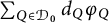 $\sum _{Q\in \mathcal {D}_0} d_Q \varphi _Q$
belongs to
 $\mathrm {J}_{s}(\mathbf {bmo}),$
where r is the regularity of the chosen wavelet basis and the sequence
 $\{d_Q\}_{Q\in \mathcal {D}_0}$
is uniformly bounded. Hence, we only need to consider the coefficients corresponding to the wavelets
 $\psi _\omega $
for
 $\omega \in \mathcal {Q}.$
Given
 $0 < s \leq 1$
and an integer
 $n \geq 1$
, consider the space of sequences
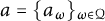 $a = \{a_\omega \}_{\omega \in \mathcal {Q}}$
with norm
 $$ \begin{align} \left\lVert a \right\rVert_{s} = \sup_{\omega \in \mathcal{Q}} 2^{|\omega|(n/2+s)} |a_\omega|. \end{align} $$
Observe that this is the same as the norm defined in formula (7) of Theorem B when
 $d_Q(f) = 0$
for all
 $Q \in \mathcal {D}_0.$
Thus, this sequence space is the space of wavelet coefficients
 $\{c_\omega \}$
(corresponding to wavelets
 $\psi _\omega $
) of functions in
 $\Lambda _{s}(\mathbb {R}^n).$
Moreover, by Theorem B, we have that
 $\left \lVert \{a_\omega \} \right \rVert _{s} \simeq \left \lVert f \right \rVert _{\Lambda _{s}}$
where
 $$ \begin{align*} f = \sum_{\omega\in\mathcal{Q}} a_\omega \psi_\omega. \end{align*} $$
In the rest of this section, we use
 $\left \lVert \cdot \right \rVert _{s}$
to denote both the norm on sequences defined by (12) and the norm equivalent to
 $\left \lVert f \right \rVert _{\Lambda _{s}}$
for functions
 $f \in \Lambda _{s}(\mathbb {R}^n)$
such that
 $d_Q(f) = 0$
for all
 $Q \in \mathcal {D}_0.$
Proof of Theorem 3 Denote by
 $\varepsilon _0$
the infimum in (9), which we assume to be positive, and assume that
 $\varepsilon < \varepsilon _0.$
Consider a function
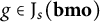 $g \in \mathrm {J}_{s}(\mathbf {bmo})$
, and assume that
 $\left \lVert f-g \right \rVert _{s} \leq \varepsilon $
(so that
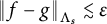 $\left \lVert f-g \right \rVert _{\Lambda _{s}} \lesssim \varepsilon $
). Note that we may also assume that
 $d_Q(g) = d_Q(f)$
for all
 $Q \in \mathcal {D}_0.$
Pick
 $\varepsilon ' \in (\varepsilon , \varepsilon _0)$
, and note that, for
 $\omega \in \mathcal {Q},$
whenever
 $|c_\omega (f)|> \varepsilon ' 2^{-|\omega |(n/2+s)},$
we have that
 $|c_\omega (g)|> \delta 2^{-|\omega |(n/2+s)},$
where
 $\delta = \varepsilon ' - \varepsilon> 0.$
Thus, for any cube
 $Q \in \mathcal {D},$
we have that
 $$ \begin{align*} \frac{1}{|Q|} \sum_{\omega\in\mathcal{Q}(Q)} 4^{s|\omega|}|c_\omega(g)|^2 &\gtrsim \frac{\delta^2}{|Q|} \sum_{\substack{P \in W(s,f,\varepsilon')\\ P \subseteq Q}} 2^{-n\tau(P)} = \frac{\delta^2}{|Q|} \sum_{\substack{P \in W(s,f,\varepsilon')\\ P \subseteq Q}} |P|\\ &\simeq \frac{\delta^2}{|Q|} \int_Q \int_0^{l(Q)} \chi_{T(s,f,\varepsilon')}(x,y)\, \frac{dy\, dx}{y}. \end{align*} $$
But the supremum, with Q ranging over all dyadic cubes, of the latter quantity is not finite, because
 $\varepsilon ' < \varepsilon _0.$
By Theorem 2, this contradicts that
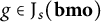 $g \in \mathrm {J}_{s}(\mathbf {bmo})$
and, thus,
 $\mathrm {dist}_s(f,\mathrm {J}_{s}(\mathbf {bmo})) \gtrsim \varepsilon _0.$
If
 $\varepsilon> \varepsilon _0,$
we construct a function
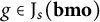 $g \in \mathrm {J}_{s}(\mathbf {bmo})$
such that
 $\mathrm {dist}_s (f,g) \lesssim \varepsilon .$
Given the wavelet coefficients
 $\{d_Q(f)\}$
and
 $\{c_\omega (f)\}$
of
 $f,$
we set
 $d_Q(g) = d_Q(f)$
for every
 $Q \in \mathcal {D}_0.$
Clearly, because
 $f \in \Lambda _{s}$
, we have that
 $$ \begin{align} \sup_{Q \in \mathcal{D}_0} |d_Q(g)| < \infty \end{align} $$
by Theorem B. Next, take
 $c_\omega (g) = c_\omega (f)$
whenever
 $\omega = (l,P)$
with
 $P \in W(s,f,\varepsilon ),$
and
 $c_\omega (g) = 0$
otherwise. By construction, we have
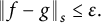 $\left \lVert f-g \right \rVert _{s} \leq \varepsilon .$
Thus, by Theorem B, we find that
 $\mathrm {dist}_s (f,g) \lesssim \varepsilon .$
Furthermore, we have that
 $$ \begin{align*} \frac{1}{|Q|} \sum_{\omega\in\mathcal{Q}(Q)} 4^{|\omega|s}|c_\omega(g)|^2 &\lesssim \frac{\left\lVert c_\omega(f) \right\rVert_{s}^2}{|Q|} \sum_{\substack{P \in W(s,f,\varepsilon)\\ P \subseteq Q}} |P|\\ &\simeq \frac{\left\lVert c_\omega(f) \right\rVert_{s}^2}{|Q|} \int_Q \int_0^{l(Q)} \chi_{T(s,f,\varepsilon)}(x,y)\, \frac{dy\, dx}{y}. \end{align*} $$
Because
 $\varepsilon> \varepsilon _0$
, the supremum of the latter quantity when Q ranges over all dyadic cubes is finite. Hence, this and (13) imply that
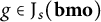 $g \in \mathrm {J}_{s}(\mathbf {bmo})$
by Theorem 2, as we wanted to show. ▪
3 Properties of the sets S, D, and T
In the present section, we first estimate local continuity properties of the various quantities defined in the upper half-space that we are using to quantify the Hölder norm. Later on, we use these estimates to control the change in the quantity
 $M(T(s,f,\varepsilon ))$
and its analogies when the corresponding set is hyperbolically enlarged.
For that purpose, let us begin by recalling some basic facts concerning the hyperbolic metric in
 $\mathbb {R}^{n +1}_+.$
The element
 $ds$
of hyperbolic arc length at
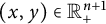 $(x,y) \in \mathbb {R}^{n +1}_+$
is defined by
 $$ \begin{align*} ds^2 = \frac{dx^2 + dy^2}{y^2}. \end{align*} $$
Geodesics in this metric are circular arcs intersecting orthogonally the hyperplane
 $\{y = 0\}$
and vertical lines, that is, straight lines intersecting orthogonally the same hyperplane. We denote by
 $\rho (a,b)$
the hyperbolic distance between
 $a,b \in \mathbb {R}^{n +1}_+$
given by this metric, that is, the hyperbolic arc length of the geodesic segment joining a and
 $b.$
Given a set
 $A \in \mathbb {R}^{n +1}_+$
and
 $R> 0,$
we will consider the R-dilation of A in the hyperbolic metric given by its hyperbolic R-neighborhood, and denote it by
 $\mathrm {dil}_{\rho }({A},{R}).$
In other words, we take
 $$ \begin{align*} \mathrm{dil}_{\rho}({A},{R}) = \{p \in \mathbb{R}^{n +1}_+\colon \rho(p,A) < R\}. \end{align*} $$
A hyperbolic ball of radius
 $r> 0$
and center
 $z \in \mathbb {R}^{n +1}_+$
is denoted by
 $\mathrm {B}_\rho ({z},{r}).$
We start by studying how
 $\Delta _2f(x,y)$
varies.
Lemma 1 Let
 $0 < s < 1.$
Consider a function
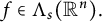 $f \in \Lambda _{s}(\mathbb {R}^n).$
Then,
 $$ \begin{align*} |\Delta_2f(x,y) - \Delta_2f(x',y')| \lesssim \left\lVert f \right\rVert_{\Lambda_{s}} \left(|x-x'|^s + |y-y'|^s\right). \end{align*} $$
Proof Consider an arbitrary auxiliary
 $p \in \mathbb {R}^n$
such that
 $|p| = y$
and note that
 $$ \begin{align*} & |(f(x+p)-f(x'+p)) - 2(f(x)-f(x')) + (f(x-p)-f(x'-p))| \\ &\quad \lesssim \left\lVert f \right\rVert_{\Lambda_{s}} |x-x'|^s, \end{align*} $$
because
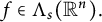 $f \in \Lambda _{s}(\mathbb {R}^n).$
Because this holds uniformly for any such
 $p,$
we may use the general fact that for a bounded function H on
 $\mathbb {R}^{2n}$
, one has that
 $$ \begin{align} \left|\sup_{|p|=y}|H(x,p)| - \sup_{|p|=y}|H(x',p)|\right| \leq \sup_{|p|=y}|H(x,p) - H(x',p)| \end{align} $$
to deduce that
 $$ \begin{align} |\Delta_2f(x,y) - \Delta_2f(x',y)| \lesssim \left\lVert f \right\rVert_{\Lambda_{s}} |x-x'|^s. \end{align} $$
On the other hand, if
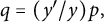 $q = (y'/y)p,$
we also have that
 $$ \begin{align*} |(f(x'+p)-f(x'+q)) + (f(x'-p)-f(x'-q))| \lesssim \left\lVert f \right\rVert_{\Lambda_{s}} |p-q|^s = \left\lVert f \right\rVert_{\Lambda_{s}} |y-y'|^s. \end{align*} $$
This is true uniformly for any such p, and, thus, it holds that
 $$ \begin{align} |\Delta_2f(x',y) - \Delta_2f(x',y')| \lesssim \left\lVert f \right\rVert_{\Lambda_{s}} |y-y'|^s. \end{align} $$
As we join (15) and (16), the conclusion follows immediately. ▪
We deal with the case
 $s = 1$
separately.
Lemma 2 Consider a function
 $f \in \Lambda _{\ast }(\mathbb {R}^n) = \Lambda _{1}(\mathbb {R}^n).$
If
 $|x-x'| < (y+y')/2,$
then
 $$ \begin{align*} |\Delta_2f(x,y) - \Delta_2f(x',y')| & \lesssim \left\lVert f \right\rVert_{\Lambda_{\ast}} \bigg(|x-x'| \log\left(e+\displaystyle\frac{y+y'}{|x-x'|}\right)\\ &\quad + |y-y'| \log\left(e+\displaystyle\frac{y+y'}{|y-y'|}\right)\bigg). \end{align*} $$
Proof Consider smooth symmetric functions
 $\widehat {\phi _0}$
and
 $\widehat {\phi _1}$
with
 $\mathrm {supp} \left ({\widehat {\phi _0}}\right ) \subseteq \{\xi \in \mathbb {R}^n\colon |\xi | \leq 1\}$
and
 $\mathrm {supp} \left ({\widehat {\phi _1}}\right ) \subseteq \{\xi \in \mathbb {R}^n\colon 1/2 \leq |\xi | \leq 2\},$
and such that if
 $\widehat {\phi _j}(\xi ) = \widehat {\phi _1}(2^{-(j-1)}\xi )$
for
 $j \in \mathbb {N},$
then
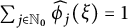 $\sum _{j\in \mathbb {N}_0} \widehat {\phi _j}(\xi ) = 1$
for every
 $\xi \in \mathbb {R}^n.$
Now, take
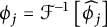 $\phi _j = \mathcal {F}^{-1}\left [{\widehat {\phi _j}}\right ]$
and
 $f_j = \phi _j \ast f$
for
 $j \in \mathbb {N}_0,$
so that the Littlewood–Paley dyadic decomposition of f can be written as
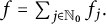 $f = \sum _{j\in \mathbb {N}_0} f_j.$
It is a well-known fact (see, for instance, [Reference SteinSte93, p. 253]) that, for a given
 $s> 0$
,
 $f \in \Lambda _{s}$
if and only if
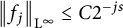 $\left \lVert f_j \right \rVert _{\mathrm {L}^{\infty }} \leq C 2^{-js}$
for all
 $j \geq 0,$
and
 $$ \begin{align*} \left\lVert f \right\rVert_{\Lambda_{s}} \simeq \sup_{j \geq 0} 2^{js} \left\lVert f_j \right\rVert_{\mathrm{L}^{\infty}}. \end{align*} $$
Moreover, we have that
 $\left \lVert \partial ^\alpha f_j \right \rVert _{\mathrm {L}^{\infty }} \leq \left \lVert f \right \rVert _{\Lambda _{s}} 2^{j|\alpha |} 2^{-js}$
for any multi-index
 $\alpha .$
In particular, this applies to the Zygmund class taking
 $s = 1.$
Take
 $p \in \mathbb {R}^n$
with
 $|p| = y$
. For this particular p, we have that
 $$ \begin{align*} &|f(x+p) - 2f(x) + f(x-p) - f(x'+p) + 2f(x') - f(x'-p)|\\ &\quad \leq \sum_{j\in\mathbb{N}_0} |f_j(x+p) - 2f_j(x) + f_j(x-p) - f_j(x'+p) + 2f_j(x') - f_j(x'-p)|. \end{align*} $$
We split this sum into those terms for which
 $2^j < 1/(y+y'),$
those with
 $1/(y+y') \leq 2^j < 1/|x-x'|$
, and those with
 $2^j \geq 1/|x-x'|.$
For the first part, we express
 $$ \begin{align*} f_j(x+p) - 2f_j(x) + f_j(x-p) = \int_{-1}^{1} (1-|u|) \frac{d^2}{du^2} f_j(x+up)\, du. \end{align*} $$
Using the bound on the third derivatives of
 $f_j$
, we obtain
 $$ \begin{align*} \left|\frac{d^2}{du^2}f_j(x+up) - \frac{d^2}{du^2}f_j(x'+up)\right| \lesssim \left\lVert f \right\rVert_{\Lambda_{\ast}} |p|^2 2^{2j}|x-x'|. \end{align*} $$
Hence,
 $$ \begin{align*} |f_j(x+p) - 2f_j(x) + f_j(x-p) - f_j(x'+p) + 2f_j(x') &- f_j(x'-p)|\\ &\lesssim \left\lVert f \right\rVert_{\Lambda_{\ast}} 2^{2j} |x-x'| y^2. \end{align*} $$
This yields
 $$ \begin{align*} \begin{aligned} \displaystyle\sum_{2^j < 1/(y+y')} |f_j(x+p) - 2f_j(x) + f_j(x-p) &- f_j(x'+p) + 2f_j(x') - f_j(x'-p)|\\ &\lesssim \left\lVert f \right\rVert_{\Lambda_{\ast}} |x-x'| y^2 \displaystyle\sum_{2^j < 1/(y+y')} 2^{2j}\\ &\lesssim \left\lVert f \right\rVert_{\Lambda_{\ast}} |x-x'|. \end{aligned} \end{align*} $$
When
 $1/(y+y') \leq 2^j < 1/|x-x'|,$
we use the j-independent uniform bound for the first derivative of
 $f_j$
to obtain directly
 $$ \begin{align*} |f_j(x+p) - 2f_j(x) + f_j(x-p) - f_j(x'+p) + 2f_j(x') &- f_j(x'-p)|\\ & \lesssim \left\lVert f \right\rVert_{\Lambda_{\ast}} |x-x'|. \end{align*} $$
Then, we find that
 $$ \begin{align*} \begin{aligned} \displaystyle\sum_{1/(y+y') \leq 2^j < 1/|x-x'|} |f_j(x+p) - 2f_j(x) &+ f_j(x-p)\\ &- f_j(x'+p) + 2f_j(x') - f_j(x'-p)|\\ &\lesssim \left\lVert f \right\rVert_{\Lambda_{\ast}} |x-x'| \displaystyle\sum_{1/(y+y') \leq 2^j < 1/|x-x'|} 1\\ &\lesssim \left\lVert f \right\rVert_{\Lambda_{\ast}} |x-x'| \log\left(e+\frac{y+y'}{|x-x'|}\right). \end{aligned} \end{align*} $$
Finally, using that
 $\left \lVert f_j \right \rVert _{\mathrm {L}^{\infty }} \lesssim \left \lVert f \right \rVert _{\Lambda _{\ast }} 2^{-j}$
, we get that the remaining terms are bounded by
 $$ \begin{align*} \begin{aligned} \displaystyle\sum_{2^j \geq 1/|x-x'|} |f_j(x+p) - 2f_j(x) &+ f_j(x-p)\\ &- f_j(x'+p) + 2f_j(x') - f_j(x'-p)|\\ &\lesssim \left\lVert f \right\rVert_{\Lambda_{\ast}} \displaystyle\sum_{2^j \geq 1/|x-x'|} 2^{-j}\\ &\lesssim \left\lVert f \right\rVert_{\Lambda_{\ast}} |x-x'|. \end{aligned} \end{align*} $$
Because all the above bounds are uniform on p with
 $|p| = y,$
applying again observation (14), we obtain the estimate
 $$ \begin{align} |\Delta_2f(x,y) - \Delta_2f(x',y)| \lesssim \left\lVert f \right\rVert_{\Lambda_{\ast}} |x-x'| \log\left(e+\frac{y+y'}{|x-x'|}\right). \end{align} $$
Now, let p be as before, and consider the case
 $x = x'$
, but
 $y \neq y'.$
We take
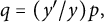 $q = (y'/y)p,$
and note that it is enough to estimate the quantity
 $$ \begin{align*} |f(x'+p) &- f(x' +q) + f(x'-p) - f(x'-q)|\\ & \leq \sum_{j\in\mathbb{N}_0} |f_j(x'+p) - f_j(x'+q) + f_j(x'-p) - f_j(x'-q)|. \end{align*} $$
We split the previous sum into those terms for which
 $2^j < 1/(y+y'),$
those with
 $1/(y+y') \leq 2^j < 1/|y-y'|$
, and those with
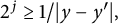 $2^j \geq 1/|y-y'|,$
and follow the previous argument with minor changes. Toward estimating the first sum, we observe first the elementary bound
 $$ \begin{align*} \begin{aligned} |g(1,1)-g(1,-1)+g(-1,-1)-g(-1,1)| &= \left|\int_{[-1,1]^2}g_{uv}(u,v)\, du\, dv\right|\\ &\leq 4 \sup_{(u,v) \in [-1,1]^2}|g_{uv}(u,v)|. \end{aligned} \end{align*} $$
As we apply this to
 $g(u,v) := f_j\left (x+u\frac {p+q}{2}+v\frac {p-q}{2}\right ),$
together with the known bound
 $\left \lVert \partial ^\alpha f_j \right \rVert _{\mathrm {L}^{\infty }} \lesssim \left \lVert f \right \rVert _{\Lambda _{\ast }} 2^j$
for multi-indices of length
 $|\alpha | = 2,$
it follows that
 $$ \begin{align*} |f_j(x'+p) - f_j(x'+q) + f_j(x'-p) - f_j(x'-q)| \lesssim \left\lVert f \right\rVert_{\Lambda_{\ast}} 2^j |y-y'| (y+y'), \end{align*} $$
and so
 $$ \begin{align*} \sum_{2^j < 1/(y+y')} |f_j(x'+p) - f_j(x'+q) + f_j(x'-p) - f_j(x'-q)| \lesssim \left\lVert f \right\rVert_{\Lambda_{\ast}} |y-y'|. \end{align*} $$
Then, for those terms with
 $1/(y+y') \leq 2^j < 1/|y-y'|,$
using the j-uniform Lipschitz property of
 $f_j$
, we may deduce
 $$ \begin{align*} |f_j(x'+p) - f_j(x'+q) + f_j(x'-p) - f_j(x'-q)| \lesssim \left\lVert f \right\rVert_{\Lambda_{\ast}} |y-y'|, \end{align*} $$
which yields
 $$ \begin{align*} \sum_{1/(y+y') \leq 2^j < 1/|y-y'|} |f_j(x'+p) - f_j(x'+q) &+ f_j(x'-p) - f_j(x'-q)|\\ &\lesssim \left\lVert f \right\rVert_{\Lambda_{\ast}} |y-y'| \log\left(e+\frac{y+y'}{|y-y'|}\right). \end{align*} $$
Finally, use the size estimate
 $\left \lVert f_j \right \rVert _{\mathrm {L}^{\infty }} \lesssim \left \lVert f \right \rVert _{\Lambda _{\ast }} 2^{-j}$
to get
 $$ \begin{align*} \sum_{2^j \geq 1/|y-y'|} |f_j(x'+p) - f_j(x'+q) + f_j(x'-p) - f_j(x'-q)| \lesssim \left\lVert f \right\rVert_{\Lambda_{\ast}} |y-y'|. \end{align*} $$
These bounds are uniform for any p and q such that
 $|p| = y$
and
 $q = (y'/y)p$
, and therefore, it is clear that
 $$ \begin{align} |\Delta_2f(x',y) - \Delta_2f(x',y')| \lesssim \left\lVert f \right\rVert_{\Lambda_{\ast}} |y-y'| \log\left(e+\frac{y+y'}{|y-y'|}\right). \end{align} $$
As a second step, we study the variation of
 $y^2 (\partial ^2 \mathrm {P}\left [{f}\right ]/\partial y^2)(x,y).$
Lemma 3 Let
 $0 < s \leq 1$
, and consider a function
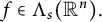 $f \in \Lambda _{s}(\mathbb {R}^n).$
Denote by u the harmonic extension
 $\mathrm {P}\left [{f}\right ]$
of f to
 $\mathbb {R}^{n +1}_+.$
Then, for any
 $(x,y),(x',y') \in \mathbb {R}^{n +1}_+,$
we have that
 $$ \begin{align*} \left|y^{2-s}\frac{\partial^2 u}{\partial y^2}(x,y) - {y'}^{2-s}\frac{\partial^2 u}{\partial y^2}(x',y')\right| \lesssim \left\lVert f \right\rVert_{\Lambda_{s}} \rho\left((x,y),(x',y')\right). \end{align*} $$
Proof Recall that
 $$ \begin{align*} \left|y^{2-s}\frac{\partial^2 u}{\partial y^2}\right| \lesssim \left\lVert f \right\rVert_{\Lambda_{s}}. \end{align*} $$
Moreover, this is equivalent to
 $$ \begin{align} \left|y^{l-s}\frac{\partial^l u}{\partial y^l}\right| \leq C_l \left\lVert f \right\rVert_{\Lambda_{s}} \end{align} $$
for any integer
 $l> 2$
(see [Reference SteinSte71, Chapter V]), where
 $C_l$
only depends on
 $l.$
Define the function
 $$ \begin{align*} g(x,y) = y^{2-s} \frac{\partial^2 u}{\partial y^2}(x,y), \end{align*} $$
and let us denote by
 $\mathrm {D}g$
the gradient of
 $g.$
Then, the hyperbolic derivative of g may be estimated in view of (19) as
 $$ \begin{align*} |y \mathrm{D}g(x,y)| &\leq y \left(\left|\frac{\partial g}{\partial y}(x,y)\right| +\sum_{k=1}^n \left|\frac{\partial g}{\partial x_k}(x,y)\right|\right)\\ &\leq (2-s) y^{2-s} \left|\frac{\partial^2 u}{\partial y^2}(x,y)\right| + y^{3-s} \left|\frac{\partial^3 u}{\partial y^3}(x,y)\right|\\ &\quad + y^{3-s} \sum_{k=1}^n \left|\frac{\partial^3 u}{\partial y^2 \partial x_k}(x,y)\right|\\ &\lesssim \left\lVert f \right\rVert_{\Lambda_{s}}. \end{align*} $$
Hence, g is locally Lipschitz with respect to the hyperbolic metric, which also implies the global Lipschitz property as the hyperbolic metric is geodesic. This implies the claim. ▪
Recall from (5) that for a given measurable set
 $A \subseteq \mathbb {R}^{n +1}_+$
, we defined the quantity
 $$ \begin{align} M(A) = \sup_{Q\in\mathcal{D}} \frac{1}{|Q|} \int_Q\int_0^{l(Q)} \chi_{A}(x,y)\, \frac{dy\, dx}{y}. \end{align} $$
Lemma 4 Assume that
 $A\subset \mathbb {R}^{n+1}_+$
has the following measure density property: there are
 $\delta ,\delta '\in (0,1/10)$
, so that the hyperbolic
 $\delta $
-neighborhood of any point
 $z\in A$
satisfies
 $$ \begin{align*} |\mathrm{B}_\rho({z},{\delta}) \cap A|\geq \delta'|\mathrm{B}_\rho({z},{\delta})|. \end{align*} $$
Then, if
 $M(A)<\infty $
, we also have
 $M(\mathrm {dil}_{\rho }({A},{R})) < \infty $
for any
 $R> 0.$
Proof For any cube
 $Q \subset \mathbb {R}^n$
, we denote
 $\widetilde Q := Q \times (0,l(Q)) \subset \mathbb {R}^{n +1}_+,$
and by
 $Q' = 3Q$
the cube that is concentric to Q and that has
 $l(Q') = 3 l(Q).$
We also denote by
 $\mu $
the Borel measure on
 $\mathbb {R}^{n +1}_+$
with density
 $d\mu = \chi _{\{0 < y \leq 1\}} y^{-1}\, dx\, dy.$
Observe that, with this notation at hand, the integral appearing in (20) for a given cube
 $Q \in \mathcal {D}$
is the same as
 $\mu (\widetilde {Q} \cap A).$
Thus, the assumption that
 $M(A)$
is finite is now equivalent to
 $$ \begin{align} \mu(\widetilde{Q} \cap A) \leq C|Q| \end{align} $$
for all
 $Q \in \mathcal {D}.$
Condition (21) is stated only for dyadic cubes with
 $l(Q) \leq 1,$
but it immediately extends to all cubes of arbitrary size with another constant
 $C.$
Let us then fix a dyadic cube
 $Q \subset \mathbb {R}^n$
with side length at most
 $1.$
Choose (via Zorn Lemma or by an elementary argument) a maximal subset
 $\mathcal {P}$
of
 $\widetilde {Q} \cap A$
such that
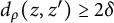 $d_\rho (z,z') \geq 2\delta $
for any distinct
 $z,z' \in \mathcal {P}.$
Then, the (open) balls
 $\mathrm {B}_\rho ({z},{\delta })$
,
 $z \in \mathcal {P},$
are disjoint, and, because
 $\delta < 1/10,$
we have directly by construction and the measure density condition of A that
 $$ \begin{align*} \mu(\mathrm{B}_\rho({z},{\delta})) \lesssim (1/\delta') \mu(\mathrm{B}_\rho({z},{\delta}) \cap A) \quad \text{for all } z \in \mathcal{P}. \end{align*} $$
Here, we used that, for
 $\delta < 1/10,$
the
 $\mu $
-measure of the hyperbolic ball
 $\mathrm {B}_\rho ({z},{\delta })$
is comparable, up to a multiplicative constant, to its Lebesgue measure in the upper half-space. Clearly,
 $\bigcup _{z \in \mathcal {P}} \mathrm {B}_\rho ({z},{\delta }) \subset \widetilde {Q'}$
, whence we obtain
 $$ \begin{align} \begin{aligned} \displaystyle\sum_{z \in \mathcal{P}} \mu(\mathrm{B}_\rho({z},{\delta})) &\lesssim (1/\delta') \displaystyle\sum_{z \in \mathcal{P}} \mu(\mathrm{B}_\rho({z},{\delta}) \cap A)\\ &\leq (1/\delta') \mu(A \cap \widetilde{Q'}) \leq (1/\delta') C |Q'| \lesssim C |Q|. \end{aligned} \end{align} $$
For any
 $R> 0,$
we have that
 $\mathrm {dil}_{\rho }({\mathrm {B}_\rho ({z},{\delta })},{R}) = \mathrm {B}_\rho ({z},{\delta + R}).$
Thus, because the
 $\mu $
-measure of a hyperbolic ball only depends on its radius, we have
 $\mu (\mathrm {dil}_{\rho }({\mathrm {B}_\rho ({z},{\delta })},{R})) \leq c(R) \mu (\mathrm {B}_\rho ({z},{\delta })),$
where
 $c(R) < \infty $
is independent of
 $z.$
Because
 $\mathcal {P}$
is
 $2\delta $
-dense in
 $\widetilde {Q} \cap A$
, we finally infer that
 $$ \begin{align*} \mu(\mathrm{dil}_{\rho}({A},{R}) \cap \widetilde{Q}) &\leq \sum_{z \in \mathcal{P}} \mu(\mathrm{dil}_{\rho}({\mathrm{B}_\rho({z},{\delta})},{3\delta+R})) \leq c(R+3\delta) \sum_{z \in \mathcal{P}} \mu(\mathrm{B}_\rho({z},{\delta}))\\ &\lesssim c(R+3\delta) C |Q|, \end{align*} $$
where we applied (22) at the last step. This shows that
 $M(\mathrm {dil}_{\rho }({A},{R})) < \infty .$
▪
For simplicity, let us now denote
 $T(\varepsilon ) = T(s,f,\varepsilon ),$
 $S(\varepsilon ) = S(s,f,\varepsilon )$
, and
 $D(\varepsilon ) = D(s,f,\varepsilon ).$
Next, we use Lemma 4 to prove useful relations between
 $T(\varepsilon )$
,
 $S(\varepsilon )$
, and
 $D(\varepsilon )$
and their hyperbolic R-neighborhoods.
Lemma 5 Let
 $0 < s \leq 1$
, and consider a function
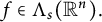 $f \in \Lambda _{s}(\mathbb {R}^n).$
Denote by
 $\varepsilon _0 = \inf \{\varepsilon> 0\colon M(T(\varepsilon )) < \infty \}.$
If
 $\varepsilon> \varepsilon _0,$
then
 $M(\mathrm {dil}_{\rho }({T(\varepsilon )},{R})) < \infty $
for any
 $R> 0.$
Proof One simply notes that an arbitrary union of upper halves of Carleson cubes obviously satisfies the condition of Lemma 4. ▪
Lemma 6 Let
 $0 < s \leq 1$
, and consider a function
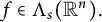 $f \in \Lambda _{s}(\mathbb {R}^n).$
Denote by
 $\varepsilon _0 = \inf \{\varepsilon> 0\colon M(S(\varepsilon )) < \infty \}.$
If
 $\varepsilon> \varepsilon _0,$
then
 $M(\mathrm {dil}_{\rho }({S(\varepsilon )},{R})) < \infty $
for any
 $R> 0.$
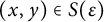
Proof Observe that, for
 $\varepsilon _0 < \varepsilon ' < \varepsilon ,$
the set
 $S(\varepsilon )$
is contained in
 $S(\varepsilon ').$
Moreover, according to Lemmas 1 and 2 (depending on if
 $s = 1$
or not), there exists
 $\eta> 0$
such that if
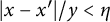 $|x-x'|/y < \eta $
and
 $1-\eta < y/y' < 1+\eta ,$
for any
 $(x,y) \in S(\varepsilon )$
, we have that
 $(x',y') \in S(\varepsilon ').$
That is to say that
 $S(\varepsilon ')$
contains a hyperbolic
 $\delta $
-neighborhood, for some
 $\delta> 0,$
of
 $S(\varepsilon )$
, and because
 $M(S(\varepsilon ')) < \infty $
, it is also true that
 $M(\mathrm {dil}_{\rho }({S(\varepsilon )},{\delta })) < \infty .$
By definition,
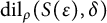 $\mathrm {dil}_{\rho }({S(\varepsilon )},{\delta })$
may be written as a union of hyperbolic balls of radius
 $\delta ,$
and hence, it clearly satisfies the condition of Lemma 4. Especially,
 $M(\mathrm {dil}_{\rho }({\mathrm {dil}_{\rho }({S(\varepsilon )},{\delta })},{R})) < \infty $
for all
 $R> 0,$
which clearly implies the claim. ▪
Lemma 7 Let
 $0 < s \leq 1$
, and consider a function
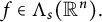 $f \in \Lambda _{s}(\mathbb {R}^n).$
Denote by
 $\varepsilon _0 = \inf \{\varepsilon> 0\colon M(D(\varepsilon )) < \infty \}.$
If
 $\varepsilon> \varepsilon _0,$
then
 $M(\mathrm {dil}_{\rho }({D(\varepsilon )},{R})) < \infty $
for any
 $R> 0.$
Proof The proof is exactly the same as in the previous lemma, one just applies instead of Lemma 3. ▪
4 Equivalence of characterizations
The aim of this section is to prove Theorems 1 and 4. For this purpose, we first show some geometric relations between the sets
 $T(\varepsilon ),$
 $S(\varepsilon )$
, and
 $D(\varepsilon ).$
Recall that for a set
 $A \subset \mathbb {R}^{n +1}_+,$
the set
 $\mathrm {dil}_{\rho }({A},{R})$
denotes the hyperbolic R-neighborhood of
 $A.$
Lemma 8 Assume that the regularity of the wavelet basis used to define the set
 $T(\varepsilon )$
is
 $r> n+3.$
Let
 $0 < s \leq 1$
, and consider a function
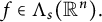 $f \in \Lambda _{s}(\mathbb {R}^n).$
There exists an absolute constant
 $c> 0$
such that, for any
 $\varepsilon> 0,$
there is
 $R = R(f,\varepsilon )> 0$
for which
 $T(\varepsilon ) \subseteq \mathrm {dil}_{\rho }({S(c\varepsilon )},{R}).$
Proof We first note that it is enough to verify for any dyadic cube
 $Q \subset \mathbb {R}^n$
with
 $l(Q) \leq 1$
that, if
 $$ \begin{align} y^{-s} \Delta_2 f(x,y) \leq \varepsilon \quad \text{for all } (x,y)\in \mathrm{dil}_{\rho}({T(Q)},{R}), \end{align} $$
then the wavelet coefficients
 $\{c_\omega (f)\}$
of f corresponding to the cube Q will satisfy
 $$ \begin{align*} \sup_{l} |c_{(l,Q)}| \lesssim \varepsilon l(Q)^{n/2+s}, \quad l = 1,\ldots,2^n-1. \end{align*} $$
First of all, we note that, without loss of generality, we can assume that
 $Q = Q_0 = [0,1]^n.$
Namely, the general result can be reduced to this case by a translation and a rescaling, because both the second differences and the wavelet coefficients behave well with respect to these operations. Recall also that our wavelets
 $\{\psi _{(l,Q_0)}\}$
have regularity
 $r> s$
and are compactly supported, say
 $\mathrm {supp} \left ({\psi _{(l,Q_0)}}\right ) \subset B(0,R_0)$
for all
 $l \in \{1,\ldots ,2^n-1\}.$
Moreover, the wavelet functions satisfy
 $$ \begin{align*} \int_{\mathbb{R}^n} x^\alpha \psi_{(l,Q_0)}(x)\, dx = 0 \end{align*} $$
for multi-indices of length
 $0 \leq |\alpha | \leq r,$
or in other words, their Fourier transforms satisfy
 $\partial ^\alpha \widehat {\psi _{(l,Q)}}(0) = 0$
for these multi-indices. Because
 $\psi _{(l,Q_0)}$
has compact support, we have that
 $\widehat {\psi _{(l,Q_0)}} \in \mathcal {C}^\infty (\mathbb {R}^n).$
Moreover, for any given multi-index
 $\beta $
, the function
 $x^\beta \psi _{(l,Q_0)}(x) \in \mathcal {C}^r(\mathbb {R})$
has compact support, so that
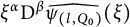 $\xi ^{\alpha } \mathrm {D}^\beta \widehat {\psi _{(l,Q_0)}}(\xi )$
is bounded for all
 $|\alpha | \leq r.$
This implies that
 $$ \begin{align} \left|\mathrm{D}^\beta \widehat{\psi_{(l,Q_0)}}(\xi)\right| \leq C_\beta (1+|\xi|)^{-r} \quad \text{for all multi-indices } \beta. \end{align} $$
Consider a nonnegative and radially symmetric
 $\mathcal {C}^\infty _0$
function g supported on the annulus
 $\{x \in \mathbb {R}^n\colon 1/2 \leq |x| \leq 2\},$
and with integral
 $1.$
Then,
 $\widehat {g}(\xi )$
is real, smooth, and radially symmetric. Moreover, from the fact that g is nonnegative, and in
 $\mathrm {L}^{1}(\mathbb {R}^n)$
, we deduce that
 $\widehat {g}(\xi ) \leq \widehat {g}(0) = 1$
for all
 $\xi \in \mathbb {R}^n.$
Furthermore, we get a quantitative version of this statement: there is a positive constant
 $c> 0$
, so that
 $$ \begin{align} 1 - \widehat{g}(\xi) \geq c \min(1,|\xi|^2)\quad \text{for }\, \xi \in \mathbb{R}^n. \end{align} $$
Indeed, for
 $\xi $
at a neighborhood of the origin, we have that
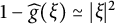 $1-\widehat {g}(\xi ) \simeq |\xi |^2$
, because g has zero first moments due to its symmetry and
 $\Delta \widehat {g}(0) = -\int _{\mathbb {R}^n} |x|^2 g(x)\, dx < 0.$
On the other hand, because g is smooth, we also have
 $1-\widehat {g}(\xi ) \simeq 1$
as
 $\xi \to \infty $
due to the fast decay of
 $\widehat {g}.$
Finally, observe that
 $\widehat {g}(\xi ) = 1$
only if
 $\xi = 0.$
This follows from the fact that g is a nonnegative radially symmetric function and that
 $e^{i2\pi x\cdot \xi }$
is constant as a function of x on the whole set
 $\{g \neq 0\}$
only for
 $\xi = 0,$
so that for
 $\xi \neq 0$
, we have that
 $$ \begin{align*} \left|\int g(x) e^{i2\pi x\cdot\xi}\, dx\right| < \int g(x)\, dx = \widehat{g}(0) = 1. \end{align*} $$
Given one of the wavelets
 $\psi _{(l,Q_0)},$
we define the function h via its Fourier transform by setting
 $$ \begin{align*} \widehat{h}(\xi) = -\frac{\widehat{\psi_l}(\xi)}{\overline{\widehat{g}(0)}-\overline{\widehat{g}(\xi)}}. \end{align*} $$
Note that, because of (25) and the fact that the derivatives of
 $\widehat {\psi _{(l,Q_0)}}$
vanish up to order at least
 $r,$
if we take r large enough, say
 $r> n+3,$
then
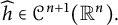 $\widehat {h} \in \mathcal {C}^{n+1}(\mathbb {R}^n).$
Moreover, all the derivatives of
 $\widehat {h}$
up to order
 $n+1$
are integrable because of the decay (24) of the derivatives of
 $\widehat {\psi _{(l,Q_0)}}$
and the uniform boundedness of each derivative of
 $\widehat {g}.$
All this implies that h is continuous and
 $(1+|x|^2)^{(n+1)/2}h(x)$
is bounded. In particular, h itself is bounded and integrable.
We are now able to estimate the wavelet coefficient in terms of the second differences:
 $$ \begin{align*} \int_{\mathbb{R}^n} \overline{\psi_{(l,Q_0)}(x)}f(x)\, dx &= (2\pi)^{-n} \int_{\mathbb{R}^n} \overline{\widehat{\psi_{(l,Q_0)}}(\xi)}\widehat{f}(\xi)\, d\xi\\ &= \int_{\mathbb{R}^n} \overline{\widehat{h}(\xi)} (\widehat{g}(\xi)-\widehat{g}(0)) \widehat{f}(\xi)\, d\xi. \end{align*} $$
Note as well that, because of the properties of g and
 $h,$
it holds that
 $$ \begin{align*} \int_{\mathbb{R}^n}\int_{\mathbb{R}^n} \overline{h(u)}&g(w)f(u+w)\, du\, dw\\ &= \int_{\mathbb{R}^n}\int_{\mathbb{R}^n} \overline{h(u)}g(w)f(u-w)\, du\, dw\\ &= \int_{\mathbb{R}^n} \overline{h(u)} (g \ast f)(u)\, du = (2\pi)^{-n} \int_{\mathbb{R}^n} \overline{\widehat{h}(\xi)} \widehat{g}(\xi)\widehat{f}(\xi)\, d\xi \end{align*} $$
and
 $$ \begin{align*} \int_{\mathbb{R}^n}\int_{\mathbb{R}^n} g(w)\overline{h(u)}f(u)\, du\, dw = (2\pi)^{-n} \widehat{g}(0) \int_{\mathbb{R}^n} \overline{\widehat{h}(\xi)}\widehat{f}(\xi)\, d\xi. \end{align*} $$
Therefore, noting also that g is bounded and supported in the annulus
 $\{x \in \mathbb {R}^n\colon 1/2 \leq |x| \leq 2\},$
we obtain
 $$ \begin{align*} \bigg|\int &\overline{\psi_l(x)}f(x)\, dx\bigg|\\ \leq &\frac{1}{2} \int_{\mathbb{R}^n}\int_{\mathbb{R}^n} |h(u) g(w)|\, |f(u+w)-2f(u)+f(u-w)|\, du\, dw\\ \leq &c_n \int_{(1/2,2)}\int_{\mathbb{R}^n} |h(u)| \Delta_2f(u,t)\, du\, dt. \end{align*} $$
Consider the set
 $A = \{(u,t)\in \mathbb {R}^{n +1}_+\colon |u| < R/2, 1/2 < t < 2\} \subset \mathrm {dil}_{\rho }({T(Q_0)},{R}),$
where we can assume (23). Note that
 $$ \begin{align*} \iint_{\mathbb{R}^{n +1}_+ \setminus A} |h(u)|\Delta_2f(u,t)\, du\, dt \leq \left\lVert f \right\rVert_{\Lambda_{s}}2^s \int_{|u| \geq R/2} |h(u)|\, du \lesssim \varepsilon \end{align*} $$
for
 $R = R(f,\varepsilon )$
large enough. On the other hand, we have by (23) that
 $$ \begin{align*} \iint_{A} |h(u)|\Delta_2f(u,t)\, du\, dt \leq \varepsilon 2^s \int_{|u| \leq R/2 } |h(u)|\, du \lesssim \varepsilon. \end{align*} $$
Moreover, thus, we get that
 $|c_{(l,Q_0)}(f)| \lesssim \varepsilon ,$
as we wanted to show. ▪
Recall that for a function
 $f \in \Lambda _{s}$
with
 $0 < s \leq 1,$
and for any integer
 $k \geq 2,$
one has that the single condition
 $$ \begin{align*} y^{2-s} \left|\frac{\partial^2 \mathrm{P}\left[{f}\right]}{\partial y^2}(x,y)\right| \lesssim \left\lVert f \right\rVert_{\Lambda_{s}} \end{align*} $$
is equivalent to
 $$ \begin{align} y^{k-s} \left|\partial^\alpha \mathrm{P}\left[{f}\right] (x,y)\right| \leq C_k \left\lVert f \right\rVert_{\Lambda_{s}}, \end{align} $$
for all multi-indices
 $\alpha $
with
 $|\alpha | = k$
and with
 $C_k$
depending only on k (see, for example, [Reference SteinSte71, pp. 143–145]). Before we establish the analogue of Lemma 8 for
 $S(\varepsilon )$
in terms of
 $\mathrm {dil}_{\rho }({D(c\varepsilon )},{R}),$
we need the following auxiliary result. For the reader’s convenience, we provide complete details in the proof (and also for analogous estimates later on) although many parts of the arguments are well known for the specialists.
Lemma 9 Let
 $0 < s \leq 1$
, and consider a function
 $f \in \Lambda _{s}$
and an integer
 $k \geq 2.$
There exists
 $R_0 = R_0(f,k)> 0$
such that if
 $R> R_0$
and
 $$ \begin{align} {y'}^{2-s} \left|\frac{\partial^2 \mathrm{P}\left[{f}\right]}{\partial y^2}(x',y')\right| \leq \varepsilon, \quad (x',y') \in \mathrm{B}_\rho({(x,y)},{R}), \end{align} $$
then
 $$ \begin{align} y^{|\alpha|-s} \left|\partial^\alpha \mathrm{P}\left[{f}\right] (x,y)\right| \lesssim \varepsilon \end{align} $$
for every multi-index
 $\alpha $
with
 $|\alpha | = k.$
Proof The arguments we use here are the same as those used to prove Lemmas 4 and 5 of [Reference SteinSte71, pp. 143–145]. We may assume that
 $R \geq 4.$
We just consider one particular multi-index, i.e., we verify that if (27) holds for R large enough, then
 $$ \begin{align} y^{2-s} \left|\frac{\partial^2 \mathrm{P}\left[{f}\right]}{\partial y \partial x_1} (x,y)\right| \lesssim \varepsilon. \end{align} $$
The general result then follows by an extension of the argument in this special case.
Let us denote
 $u(x,y) = \mathrm {P}\left [{f}\right ](x,y).$
Using that, for
 $y> 0$
, the Poisson kernel satisfies
 $P_y(x) = (P_{y/2} \ast P_{y/2})(x),$
one can express
 $u(x,y) = (P_{y/2} \ast u_{y/2})(x),$
where
 $u_y(t) = u(t,y).$
Thus, one gets
 $$ \begin{align*} \frac{\partial^3 u}{\partial^2 y \partial x_1} = \frac{\partial P_{y/2}}{\partial x_1} \ast \frac{\partial^2 u}{\partial y^2}\bigg|_{y/2}. \end{align*} $$
Next, write
 $$ \begin{align*} \begin{aligned} \left|\displaystyle\frac{\partial^3 u}{\partial^2 y \partial x_1} (x',y')\right| &\leq \displaystyle\int_{|w| \leq (R/4)y'} \left|\displaystyle\frac{\partial P_{y'/2}}{\partial x_1}(w)\right|\, \left|\displaystyle\frac{\partial^2 u}{\partial y^2}(x'-w,y'/2)\right|\, dw \\ &\quad + \displaystyle\int_{|w|> (R/4)y'} \left|\displaystyle\frac{\partial P_{y'/2}}{\partial x_1}(w)\right|\, \left|\displaystyle\frac{\partial^2 u}{\partial y^2}(x'-w,y'/2)\right|\, dw. \end{aligned} \end{align*} $$
Thus, because in the first term above we can assume that
 $(x'-w',y'/2) \in \mathrm {B}_\rho ({(x,y)},{R}),$
we obtain
 $$ \begin{align*} \int_{|w| \leq \widetilde{R}y'} \left|\frac{\partial P_{y'/2}}{\partial x_1}(w)\right|\, \left|\frac{\partial^2 u}{\partial y^2}(x'-w,y'/2)\right|\, dw \lesssim \varepsilon {y'}^{s-3} \end{align*} $$
for the first term, whereas for the second one it is easily checked by scaling that
 $\int _{|x|\geq Ay}|\partial P_y/\partial x_1| \lesssim (Ay)^{-1},$
so that
 $$ \begin{align*} \int_{|w|> \widetilde{R}y'} \left|\frac{\partial P_{y'/2}}{\partial x_1}(w)\right|\, \left|\frac{\partial^2 u}{\partial y^2}(x'-w,y'/2)\right|\, dw \lesssim \frac{\left\lVert f \right\rVert_{\Lambda_{s}}}{\widetilde{R}} {y'}^{s-3}. \end{align*} $$
Summing up, if
 $\widetilde {R}$
is large enough, we have that
 $$ \begin{align} \left|\frac{\partial^3 u}{\partial^2 y \partial x_1} (x',y')\right| \lesssim \varepsilon {y'}^{s-3} \end{align} $$
for all
 $(x',y') \in \mathrm {B}_\rho ({(x,y)},{R'}),$
for
 $R'> 0$
possibly smaller than
 $R,$
but also arbitrarily large.
Now, taking into account that f is uniformly bounded and that the Poisson kernel satisfies
 $\left \lVert (\partial ^2 P_y/\partial y \partial x_1) \right \rVert _{\mathrm {L}^{1}} \lesssim y^{-2},$
we have that
 $$ \begin{align*} \left|\frac{\partial^2 u}{\partial y \partial x_1}(x,y)\right| \lesssim y^{-2} \left\lVert f \right\rVert_{\mathrm{L}^{\infty}}, \end{align*} $$
from which it follows that
 $|(\partial ^2 u/\partial y \partial x_1) (x,y)|$
tends to zero as
 $y \to \infty .$
Hence, one can express
 $$ \begin{align*} \begin{aligned} \left|\frac{\partial^2 u}{\partial y \partial x_1}(x,y)\right| &\leq \int_y^\infty \left|\frac{\partial^3 u}{\partial y^2 \partial x_1}(x,y')\right| \, dy'\\ &= \int_y^{R'y} \left|\frac{\partial^3 u}{\partial y^2 \partial x_1}(x,y')\right| \, dy' + \int_{R'y}^\infty \left|\frac{\partial^3 u}{\partial y^2 \partial x_1}(x,y')\right| \, dy'. \end{aligned} \end{align*} $$
Using (30) on the first term, and noting that
 $\rho ((x,ty),(x,y)) \leq R'$
for
 $t \in (1,R'),$
we get the bound
 $$ \begin{align*} \int_y^{R'y} \left|\frac{\partial^3 u}{\partial y^2 \partial x_1}(x,y')\right| \, dy' \lesssim \varepsilon \int_y^{R'y} {y'}^{s-3}\, dy' \leq \varepsilon y^{s-2}. \end{align*} $$
For the second term, we get
 $$ \begin{align*} \int_{R'y}^\infty \left|\frac{\partial^3 u}{\partial y^2 \partial x_1}(x,y')\right| \, dy' \lesssim \left\lVert f \right\rVert_{\Lambda_{s}} \int_{R'y}^\infty {y'}^{s-3}\, dy' = \frac{\left\lVert f \right\rVert_{\Lambda_{s}}}{{R'}^{2-s}} y^{s-2} \end{align*} $$
using the bound
 $y^{3-s}|(\partial ^3 u/\partial y^2 \partial x_1) (x,y)| \lesssim \left \lVert f \right \rVert _{\Lambda _{s}}\!\!.$
Therefore, adding these two bounds, we get (29) by choosing
 $R'$
(and thus also R) large enough, depending on f and
 $\varepsilon ,$
as we wanted to see. ▪
Lemma 10 Let
 $0 < s \leq 1$
, and consider a function
 $f \in \Lambda _{s}.$
There exists an absolute constant
 $c> 0$
such that, for any
 $\varepsilon> 0,$
there is
 $R = R(f,\varepsilon )> 0$
for which
 $S(\varepsilon ) \subseteq \mathrm {dil}_{\rho }({D(c\varepsilon )},{R}).$
Proof We may assume that
 $R \geq 4.$
Fix
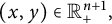 $(x,y) \in \mathbb {R}^{n +1}_+,$
and let us denote
 $u = \mathrm {P}\left [{f}\right ].$
We need to see that, if
 $$ \begin{align} {y'}^{2-s} \left|\frac{\partial^2 u}{\partial y^2}(x',y')\right| \leq \varepsilon \end{align} $$
for every
 $(x',y') \in \mathrm {B}_\rho ({(x,y)},{R}),$
then
 $$ \begin{align} \frac{\Delta_2f(x,y)}{y^s} \lesssim \varepsilon. \end{align} $$
Let us fix
 $p = (p_1,\ldots ,p_n)$
with
 $|p| = 1.$
If f was twice continuously differentiable, we would write
 $$ \begin{align} \begin{aligned} f(x+yp) - 2f(x) &+ f(x-yp)|\\ &= \displaystyle\int_0^y\int_{-h}^h \displaystyle\frac{d^2}{dt^2}f(x+ tp)\, dt\, dh\\ &= \displaystyle\int_0^y\int_{-h}^h \left(\displaystyle\sum_{i,j=1}^n p_i p_j \displaystyle\frac{\partial^2 f}{\partial x_i \partial x_j}\right)\, dt\, dh. \end{aligned} \end{align} $$
Note that, for
 $f \in \Lambda _{s}$
, we can express
 $$ \begin{align*} f(x) = \int_0^y y'\frac{\partial^2 u}{\partial y^2}(x,y')\, dy' - y\frac{\partial u}{\partial y}(x,y) + u(x,y) \end{align*} $$
for any
 $y> 0$
. Thus, we can express the second difference of f as
 $$ \begin{align} \begin{aligned} |f(x+yp) &- 2f(x) + f(x-yp)|\\ &\leq \displaystyle\int_0^y y'\left|\displaystyle\frac{\partial^2 u}{\partial y^2}(x+yp,y') -2\displaystyle\frac{\partial^2 u}{\partial y^2}(x,y') +\displaystyle\frac{\partial^2 u}{\partial y^2}(x-yp,y')\right|\, dy'\\ &\quad +y\left|\displaystyle\frac{\partial u}{\partial y}(x+yp,y) -2\displaystyle\frac{\partial u}{\partial y}(x,y) +\displaystyle\frac{\partial u}{\partial y}(x-yp,y)\right|\\ &\quad +|u(x+yp,y) -2u(x,y) +u(x-yp,y)|. \end{aligned} \end{align} $$
We focus first on the integral term in (34). Because of (31), we can assume that
 $$ \begin{align*} \left|\frac{\partial^2 u}{\partial y^2}(x',y')\right| \leq \varepsilon {y'}^{-2+s} \end{align*} $$
for
 $2y/R < y' < y$
and
 $|x-x'| < Ry/2.$
Therefore, we have that
 $$ \begin{align*} \int_{2y/R}^y y' &\left|\frac{\partial^2 u}{\partial y^2}(x+yp,y') -2\frac{\partial^2 u}{\partial y^2}(x,y') +\frac{\partial^2 u}{\partial y^2} (x -yp,y')\right|\, dy'\\ &\qquad\qquad\qquad\qquad\qquad\qquad\qquad\qquad \quad \lesssim \int_{2y/R}^y \varepsilon {y'}^{-1+s}\, dy' \lesssim \varepsilon y^s. \end{align*} $$
On the other hand, we have that
 $$ \begin{align*} \int_0^{2y/R} y' &\left|\frac{\partial^2 u}{\partial y^2}(x+yp,y') -2\frac{\partial^2 u}{\partial y^2}(x,y') +\frac{\partial^2 u}{\partial y^2}(x-yp,y')\right|\, dy'\\ &\qquad\qquad\qquad\qquad\qquad \quad \lesssim \left\lVert f \right\rVert_{\Lambda_{s}} \int_0^{2y/R} {y'}^{-1+s}\, dy' \lesssim \frac{\left\lVert f \right\rVert_{\Lambda_{s}}}{R^s} y^s, \end{align*} $$
which will be bounded by
 $\varepsilon y^s$
for R large enough, depending on f and
 $\varepsilon .$
In order to bound the second and third terms in (34), we express them using (33). Let
 $g(t,y) = (\partial u / \partial y)(t,y)$
and note that, by Lemma 9, we have
 $$ \begin{align*} \left|\frac{\partial^2 g}{\partial x_i \partial x_j}(x+ tp,y)\right| = \left|\frac{\partial^3 u}{\partial x_i \partial x_j \partial y}(x+ tp,y)\right| \lesssim \varepsilon y^{-3+s} \end{align*} $$
for
 $|t| < y$
if (31) holds for R large enough (independent of y). Thus,
 $$ \begin{align*} \begin{aligned} y\bigg|\displaystyle\frac{\partial u}{\partial y}(x+yp,y) &-2\displaystyle\frac{\partial u}{\partial y}(x,y) +\displaystyle\frac{\partial u}{\partial y}(x-yp,y)\bigg|\\ &\leq y \displaystyle\int_0^{y}\int_{-h}^h \bigg|\displaystyle\frac{d^2}{dt^2}g(x+ tp,y)\bigg|\, dt\, dh\\ &\lesssim \displaystyle\int_0^y\displaystyle\int_{-h}^h \varepsilon y^{-2+s}\, dt\, dh \lesssim \varepsilon y^s. \end{aligned} \end{align*} $$
Similarly, to bound the third term in (34), we use that
 $$ \begin{align*} \left|\frac{\partial^2 u}{\partial x_i \partial x_j}(x+ tp,y)\right| \lesssim \varepsilon y^{-2+s} \end{align*} $$
for
 $|t| < y$
if (31) holds for R large enough (independent of y), again due to Lemma 9. The same reasoning as before yields that
 $$ \begin{align*} |u(x+yp,y) -2u(x,y) +u(x-yp,y)| \lesssim \varepsilon y^s. \end{align*} $$
This shows that
 $$ \begin{align*} |f(x+yp) - 2f(x) + f(x-yp)| \lesssim \varepsilon y^s, \end{align*} $$
and, because this bound is uniform on the choice of
 $p,$
equation (32) follows. ▪
In the following lemma, we place the extra condition (35) on
 $f,$
stating that the wavelet coefficients
 $\{d_Q(f)\}$
of f corresponding to
 $\varphi _Q$
,
 $Q \in \mathcal {D}_0,$
all vanish. However, this will be irrelevant for our later applications.
Lemma 11 Assume that the regularity of the wavelet basis used to define the set
 $T(\varepsilon )$
is
 $r \geq 2.$
Let
 $0 < s \leq 1$
, and consider a function
 $f \in \Lambda _{s}$
such that
 $$ \begin{align} d_Q (f) = 0 \quad \text{for all } Q \in \mathcal{D}_0. \end{align} $$
Then, there exists an absolute constant
 $c> 0$
such that, for any
 $\varepsilon> 0,$
there is
 $R = R(f,\varepsilon )> 0$
for which
 $D(\varepsilon ) \subseteq \mathrm {dil}_{\rho }({T(c\varepsilon )},{R}).$
Proof Fix
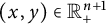 $(x,y) \in \mathbb {R}^{n +1}_+$
, and consider the set G of dyadic cubes of the form
 $Q = \{x'\in \mathbb {R}^n\colon 2^jx'-k\in [0,1]^n\}$
such that
 $y/R < 2^{-j} < yR$
and
 $|x-2^{-j}k| \lesssim 2^{-j} R,$
where R is a positive constant to be determined later. By the basic properties of the hyperbolic distance, all top half-cubes
 $T(Q)$
for
 $Q \in G$
are included in a hyperbolic neighborhood of
 $(x,y)$
in the upper half-space whose radius depends only on
 $R.$
It is hence enough to verify that, by an appropriate choice of
 $R,$
the assumption
 $$ \begin{align} \sup_l |c_{(l,Q)}(f)| \leq \varepsilon 2^{-j(n/2+s)} \end{align} $$
for every
 $Q \in G$
implies that
 $$ \begin{align} y^{2-s} \left|\frac{\partial^2 u}{\partial y^2}(x,y)\right| \lesssim \varepsilon. \end{align} $$
Recall that, by Theorem B and assumption (35), we may write
 $$ \begin{align*} f(x) = \sum_{1 \leq l \leq 2^n-1} \sum_{j\geq 0} \sum_{Q\in\mathcal{D}_j} c_{(l,Q)}(f) \psi_{(l,Q)}(x) \end{align*} $$
with
 $|c_{(l,Q)}(f)| \lesssim 2^{-j(n/2+s)} \left \lVert f \right \rVert _{\Lambda _{s}}$
when
 $Q \in \mathcal {D}_j.$
Now, for
 $j \geq 0,$
let us denote
 $$ \begin{align*} f_j(x) = \sum_{1 \leq l \leq 2^n-1} \sum_{Q\in\mathcal{D}_j} c_{(l,Q)}(f) \psi_{(l,Q)}(x), \end{align*} $$
and also consider its harmonic extension
 $u_j = \mathrm {P}\left [{f_j}\right ]$
on the upper half-space. We estimate first the contribution of
 $u_j$
to (37) for j such that
 $2^{-j}> yR.$
Of course, if y is not small enough, this range is empty and the corresponding contribution is automatically
 $0,$
and the same remark applies to some other cases considered below. Note that, by harmonicity, it is enough to bound
 $|(\partial ^2 u_j/\partial x_i^2) (x,y)|$
for
 $1 \leq i \leq n.$
First, observe that
 $$ \begin{align*} \left|\frac{\partial^2 u_j}{\partial x_i^2}(x,y)\right| = \left|\left(P_y \ast \frac{\partial^2 f_j}{\partial x_i^2}\right)(x,y)\right| \leq \left\lVert P_y \right\rVert_{\mathrm{L}^{1}} \left\lVert \frac{\partial^2 f_j}{\partial x_i^2} \right\rVert_{\mathrm{L}^{\infty}} = \left\lVert \frac{\partial^2 f_j}{\partial x_i^2} \right\rVert_{\mathrm{L}^{\infty}}. \end{align*} $$
Then, using that, for any multi-index
 $\alpha $
of length
 $|\alpha | = 2$
, we have
 $|\partial ^\alpha \psi _{(l,Q)}| \lesssim 2^{j(n/2+2)}$
for
 $Q \in \mathcal {D}_j,$
the bound on the wavelet coefficients
 $|c_{(l,Q)}|$
, and the bounded overlap of the wavelet functions (due to their compact support), we obtain
 $$ \begin{align*} \left|\frac{\partial^2 u_j}{\partial x_i^2}(x,y)\right| \lesssim \left\lVert f \right\rVert_{\Lambda_{s}} 2^{j(2-s)}. \end{align*} $$
Thus, summing over
 $j,$
for
 $2^{-j}> yR,$
we get that
 $$ \begin{align} \sum_{2^{-j}> yR} \left|\frac{\partial^2 u_j}{\partial x_i^2}(x,y)\right| \lesssim \left\lVert f \right\rVert_{\Lambda_{s}} y^{-2+s} R^{-2+s} \lesssim \varepsilon y^{-2+s}, \end{align} $$
where the last inequality holds for
 $R = R(f,\varepsilon )$
large enough (independent of
 $(x,y)$
), because
 $s \leq 1.$
Next, we compute the contribution of
 $u_j$
to (37) for j such that
 $2^{-j} \leq y/R.$
In this case, we have that
 $$ \begin{align*} \left|\frac{\partial^2 u_j}{\partial y^2}(x,y)\right| = \left|\left(\frac{\partial^2 P_y}{\partial y^2} \ast f_j\right)(x,y)\right| \leq \left\lVert \frac{\partial^2 P_y}{\partial y^2} \right\rVert_{\mathrm{L}^{1}} \left\lVert f_j \right\rVert_{\mathrm{L}^{\infty}}. \end{align*} $$
One can see by direct computation that
 $$ \begin{align} \left|\frac{\partial^2 P_y}{\partial y^2}(x,y)\right| \lesssim y^{-n-2} \left(1 + \frac{|x|^2}{y^2}\right)^{-(n+3)/2}, \end{align} $$
so in particular
 $\left \lVert (\partial ^2 P_y/\partial y^2) \right \rVert _{\mathrm {L}^{1}} \lesssim 1/y^2.$
This last estimate together with
 $\left \lVert f_j \right \rVert _{\mathrm {L}^{\infty }} \lesssim \left \lVert f \right \rVert _{\Lambda _{s}} 2^{-js},$
which holds again because of the bound on the wavelet coefficients and the bounded overlap of the wavelets themselves, shows that
 $$ \begin{align*} \left|\frac{\partial^2 u_j}{\partial y^2}(x,y)\right| \lesssim \left\lVert f \right\rVert_{\Lambda_{s}} y^{-2} 2^{-js}. \end{align*} $$
Summing now over
 $j,$
for
 $2^{-j} \leq y/R,$
we get that
 $$ \begin{align} \sum_{2^{-j} \leq y/R} \left|\frac{\partial^2 u_j}{\partial y^2}(x,y)\right| \lesssim \left\lVert f \right\rVert_{\Lambda_{s}} y^{-2+s} R^{-s} \lesssim \varepsilon y^{-2+s}, \end{align} $$
where the last inequality holds for
 $R = R(f,\varepsilon )$
large enough.
For j such that
 $y/R < 2^{-j} \leq yR,$
we express
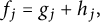 $f_j = g_j + h_j,$
where
 $$ \begin{align*} g_j(x) = \sum_{1 \leq l \leq 2^n-1} \sum_{Q\in\mathcal{D}_j\cap G} c_{(l,Q)}(f) \psi_{(l,Q)}(x). \end{align*} $$
If
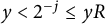 $y < 2^{-j} \leq yR$
, as we did in the case
 $yR < 2^{-j},$
we have that
 $$ \begin{align*} \left|\frac{\partial^2 u_j}{\partial x_i^2}(x,y)\right| &= \left|\left(P_y \ast \frac{\partial^2 f_j}{\partial x_i^2}\right)(x,y)\right|\\ & \leq \left|\left(P_y \ast \frac{\partial^2 g_j}{\partial x_i^2}\right)(x,y)\right| + \left|\left(P_y \ast \frac{\partial^2 h_j}{\partial x_i^2}\right)(x,y)\right|. \end{align*} $$
Because of (36), the first term is bounded by
 $C \varepsilon 2^{j(2-s)}$
. Observe that function
 $h_j$
only contains wavelets whose supports lie on the set
 $\{t\in \mathbb {R}^n\colon |t-x| \gtrsim yR\}$
. Thus, we can bound the second term by
 $$ \begin{align*} C \left\lVert \frac{\partial^2 h_j}{\partial x_i^2} \right\rVert_{\mathrm{L}^{\infty}} \int_{|t| \gtrsim yR} P_y(t)\, dt \lesssim \left\lVert f \right\rVert_{\Lambda_{s}} 2^{j(2-s)} \frac{1}{R}. \end{align*} $$
This yields, by harmonicity, that
 $$ \begin{align} \sum_{y < 2^{-j} \leq yR} \left|\frac{\partial^2 u_j}{\partial y^2}(x,y)\right| \lesssim \left(\varepsilon + \frac{\left\lVert f \right\rVert_{\Lambda_{s}}}{R}\right) y^{-2+s} \lesssim \varepsilon y^{-2+s}, \end{align} $$
where the last inequality holds for
 $R = R(f,\varepsilon )$
large enough. Similarly, if
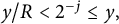 ${y/R < 2^{-j} \leq y,}$
we write
 $$ \begin{align*} \left|\frac{\partial^2 u_j}{\partial y^2} (x,y)\right| &= \left|\left(\frac{\partial^2 P_y}{\partial y^2} \ast f_j\right)(x,y)\right|\\ & \leq \left|\left(\frac{\partial^2 P_y}{\partial y^2} \ast g_j\right)(x,y)\right| + \left|\left(\frac{\partial^2 P_y}{\partial y^2} \ast h_j\right)(x,y)\right|. \end{align*} $$
Now, the first term is bounded by
 $C \varepsilon y^{-2} 2^{-js}$
because of condition (36). Taking into account that the wavelets appearing in
 $h_j$
are supported on
 $\{t\in \mathbb {R}^n\colon |t-x| \gtrsim 2^{-j} R\},$
the second term is bounded by
 $$ \begin{align*} C \left\lVert h_j \right\rVert_{\infty} \int_{|t| \gtrsim 2^{-j} R} \left|\frac{\partial^2 P_y}{\partial y^2}(t)\right|\, dt \lesssim \left\lVert f \right\rVert_{\Lambda_{s}} y 2^{j(3-s)} \frac{1}{R^3}, \end{align*} $$
where we have used equation (39) to see that
 $\int _{|x|>Ay} |(\partial ^2 P_y/\partial y^2)(t)\, dt| \lesssim y^{-2}A^{-3}.$
It follows that
 $$ \begin{align} \sum_{y/R < 2^{-j} \leq y} \left|\frac{\partial^2 u_j}{\partial y^2}(x,y)\right| \lesssim \left(\varepsilon + \frac{\left\lVert f \right\rVert_{\Lambda_{s}}}{R^s}\right) y^{-2+s} \lesssim \varepsilon y^{-2+s}, \end{align} $$
where the last inequality holds for
 $R = R(f,\varepsilon )$
large enough (and independent of
 $(x,y)$
). Because
 $u = \sum _j u_j,$
estimates (38) and (40)–(42) yield (37), as we wanted to see. ▪
Proof of Theorems 1 and 4 Let
 $0 < s \leq 1$
, and fix
 $f \in \Lambda _{s}.$
Let us denote by
 $\tau _0 = \tau _0(f)$
the infimum in (9), by
 $\sigma _0 = \sigma _0(f)$
the infimum in (6), and by
 $\delta _0 = \delta _0(f)$
the one in (11). Moreover, let c be the smallest of the constants appearing in Lemmas 8, 10, and 11. Note that we can assume that
 $c \leq 1.$
We assume as well that the wavelet basis used in Theorem 3 has regularity
 $r> n + 3$
—note that this is just for the sake of the proof below, and in the actual wavelet characterization in Theorem 3, it is enough to assume that
 $r> s.$
We first show that
 $$ \begin{align} \tau_0 \leq c^{-1} \sigma_0. \end{align} $$
To that end, note that by Lemma 6 we have that
 $M(\mathrm {dil}_{\rho }({S(\varepsilon )},{R})) < \infty $
for all
 $\varepsilon> \sigma _0$
and
 $R \geq 1.$
Then, Lemma 8 implies that
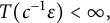 $T(c^{-1}\varepsilon ) < \infty ,$
which gives (43). Exactly in the same way, Lemmas 7 and 10 yield the inequality
 $$ \begin{align} \sigma_0 \leq c^{-1} \delta_0. \end{align} $$
Finally, in order to treat the remaining inequality, we write
 $$ \begin{align*} f = \sum_{Q \in \mathcal{D}_0} d_Q(f) \varphi_Q + \sum_{\omega \in \mathcal{Q}} c_\omega(f) \psi_\omega = g + b \end{align*} $$
and denote
 $u_g$
(resp.
 $u_b$
) the Poisson extension of g (resp. of b). Because of the (at least)
 $\mathcal {C}^2$
-regularity of the wavelets
 $\varphi _Q$
and their bounded overlap due to their compact support, we deduce that
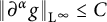 $\left \lVert \partial ^\alpha g \right \rVert _{\mathrm {L}^{\infty }} \leq C$
for every multi-index with
 $|\alpha | \leq 2.$
This implies that
 $$ \begin{align*} y^{2-s} \left|\frac{\partial^2 u_g}{\partial y^2}\right| \lesssim \min (y^{2-s},y^{-s}) \end{align*} $$
because of the estimate
 $\left \lVert \partial ^2 P_y/\partial y^2 \right \rVert _{\mathrm {L}^{1}} \lesssim y^{-2}$
and the fact that
 $\left \lVert P_y \right \rVert _{\mathrm {L}^{1}} = 1.$
Because the previous bound tends to zero uniformly as
 $y \to 0^+$
and as
 $y \to \infty ,$
we deduce immediately from the definition that
 $M(D(s,g,\varepsilon )) < \infty $
for every
 $\varepsilon> 0.$
Now, for any
 $\varepsilon _1 + \varepsilon _2 \leq \varepsilon $
, we have that
 $$ \begin{align*} M(D(s,f,\varepsilon)) \leq M(D(s,g,\varepsilon_1)) + M(D(s,b,\varepsilon_2)), \end{align*} $$
so we deduce that
 $\delta _0(f) \leq \delta _0(b).$
On the other hand, we have that
 $\tau _0(f) = \tau _0(b)$
by definition, and Lemma 11 applies to the function
 $b,$
so that with this and Lemma 5, we deduce as before that
 $$ \begin{align} \delta_0 \leq \delta_0(b) \leq c^{-1} \tau_0(b) = c^{-1} \tau_0. \end{align} $$
The proof of Theorems 1 and 4 now follows immediately from Theorem 3 and inequalities (43)–(45). ▪
Acknowledgment
We would like to thank Óscar Domínguez, Eugenio Hernández, Oleg Ivrii, and Artur Nicolau for helpful comments and conversations on the topic. We are also indebted to the referees for their valuable comments which have substantially improved the presentation of the paper.



