1 Introduction
The hemispheric-scale meridional transport of abyssal water masses is the principal mechanism by which cold dense ocean water produced in the polar regions flows back towards the equator and beyond in the deep ocean. In the North Atlantic, the southward transport associated with the Deep Western Boundary Current (DWBC) along the North American continental slope is an example of such a flow, as is, in the South Atlantic, the northward transport associated with Antarctic Bottom Water (AABW) along the South American continental slope. These equatorward flows are a significant component of the deep part of the global thermohaline overturning circulation. Their dynamics, accordingly, plays an important role in climate evolution.
Observations (e.g. Joyce et al.
Reference Joyce, Dunworth-Baker, Pickart and Waterman2005; Cunningham et al.
Reference Cunningham, Kanzow, Rayner, Baringer, Johns, Marotzke, Longworth, Grant, Hirschi and Beal2007; Baehr et al.
Reference Baehr, Cunnningham, Haak, Heimbach, Kanzow and Marotzke2009; among many others), theoretical considerations (e.g. Edwards & Pedlosky Reference Edwards and Pedlosky1998; Swaters Reference Swaters2006a
, Reference Swaters2015a
; among others) and numerical simulations (e.g. Spall Reference Spall1994; Choboter & Swaters Reference Choboter and Swaters2004; Swaters Reference Swaters2006b
; Kim, Swaters & Sutherland Reference Kim, Swaters and Sutherland2014; among others) suggest that in mid-latitudes, away from the equator and from the polar source regions, these abyssal flows are often grounded (i.e. where the abyssal current height intersects the bottom, which is sometimes also called an ‘incropping’ in an obvious reference to outcroppings associated with surface currents) on the continental slope, in geostrophic balance, flow substantial distances coherently across the planetary vorticity gradient, are density- or gravity-driven, and are more or less topographically steered. The principal purpose of this paper is to examine these dynamics in a simple but nevertheless illuminating nonlinear time-dependent planetary geostrophic reduced-gravity model that describes density- or gravity-driven grounded abyssal meridional flow over sloping topography permitting groundings in the abyssal water height in a mid-latitude
 $\unicode[STIX]{x1D6FD}$
-plane.
We hasten to add that the model we examine here will intentionally ignore many physical processes that are important, such as baroclinic, barotropic and Kelvin–Helmholtz instability, vertical entrainment and mixing between the overlying water column and the abyssal water mass, and bottom friction (with respect to frictional spin-down, see, for example, MacCready (Reference MacCready1994)). We have examined some of these processes previously (e.g. Swaters Reference Swaters1991, Reference Swaters1998, Reference Swaters2003, Reference Swaters2009, Reference Swaters2015a ,Reference Swaters b , Reference Swaters2017). Rather, we suggest that it is of interest to understand the fundamental geophysical fluid mechanics associated with the idealized low-frequency nonlinear dynamics that the observations and numerical simulations seem to suggest dominates the mid-latitude meridional transport of abyssal water masses along a continental slope, which crosses the planetary vorticity gradient. It is not our intention to model a specific oceanographic event. Our goal here is to present a theoretical process study that describes the range of dynamics this model possesses.
The plan of the paper is as follows. In § 2 the derivation of the model and its connection to similar previously derived models is briefly described. Exact nonlinear solutions to the model can be obtained in both the steady and time-dependent limits using the method of characteristics. Section 3 describes the steady solutions to the model. It is shown that, if the flow is everywhere equatorward on the poleward boundary of the region being considered (in either the southern or northern hemisphere), then no ‘shock’ forms in the solution in the mid-latitude region of interest. The general theory is illustrated with a very simple example in which the abyssal flow corresponds to a non-parallel equatorward shear flow that possesses a single along-slope grounding in the abyssal layer height along the upslope edge of the current (Swaters (Reference Swaters2013, Reference Swaters2015a ) describes other complementary nonlinear steady solutions of the model with different physical parameters).
Section 4 describes time-dependent solutions to the initial-value or Cauchy problem associated with the nonlinear model. Two specific examples are examined in order to illustrate the exact nonlinear time-dependent solutions to the initial-value problem. The first corresponds to the evolution of an initially parallel along-slope flow that has no cross-slope shear but possesses a single upslope grounding. The development into a non-parallel shear flow is described. The second example corresponds to the meridional propagation and spatial evolution of an initially isolated radially symmetric abyssal dome or pool. The abyssal dome travels meridionally and unsteadily along and across the topography crossing the planetary vorticity gradient. The abyssal dome loses its initial radial symmetry and deforms into an elliptical shape while slowly diminishing in height.
Section 5 describes the solution to the time-dependent boundary-value problem in which the in-flow abyssal current along the poleward edge of the mid-latitude domain is allowed to vary in time. In this context, we examine the evolution of the downstream flow when the in-flow current, which contains both an upslope and a downslope grounding, possesses a time-dependent height, grounding locations and cross-slope axis of symmetry. Two specific examples are examined. The first corresponds to a time-limited surge in the equatorward transport along the poleward boundary. The resulting flow in the interior of the domain resembles a varicose-like anomaly within the abyssal current that propagates equatorward. The second situation examined corresponds to a time-limited downslope shift in the cross-slope position of the abyssal current’s centre of mass. The resulting flow in the interior of the domain resembles a sinuous-like downslope loop or plume anomaly that propagates equatorward. The paper is summarized in the Conclusions in § 6.
2 Governing equations
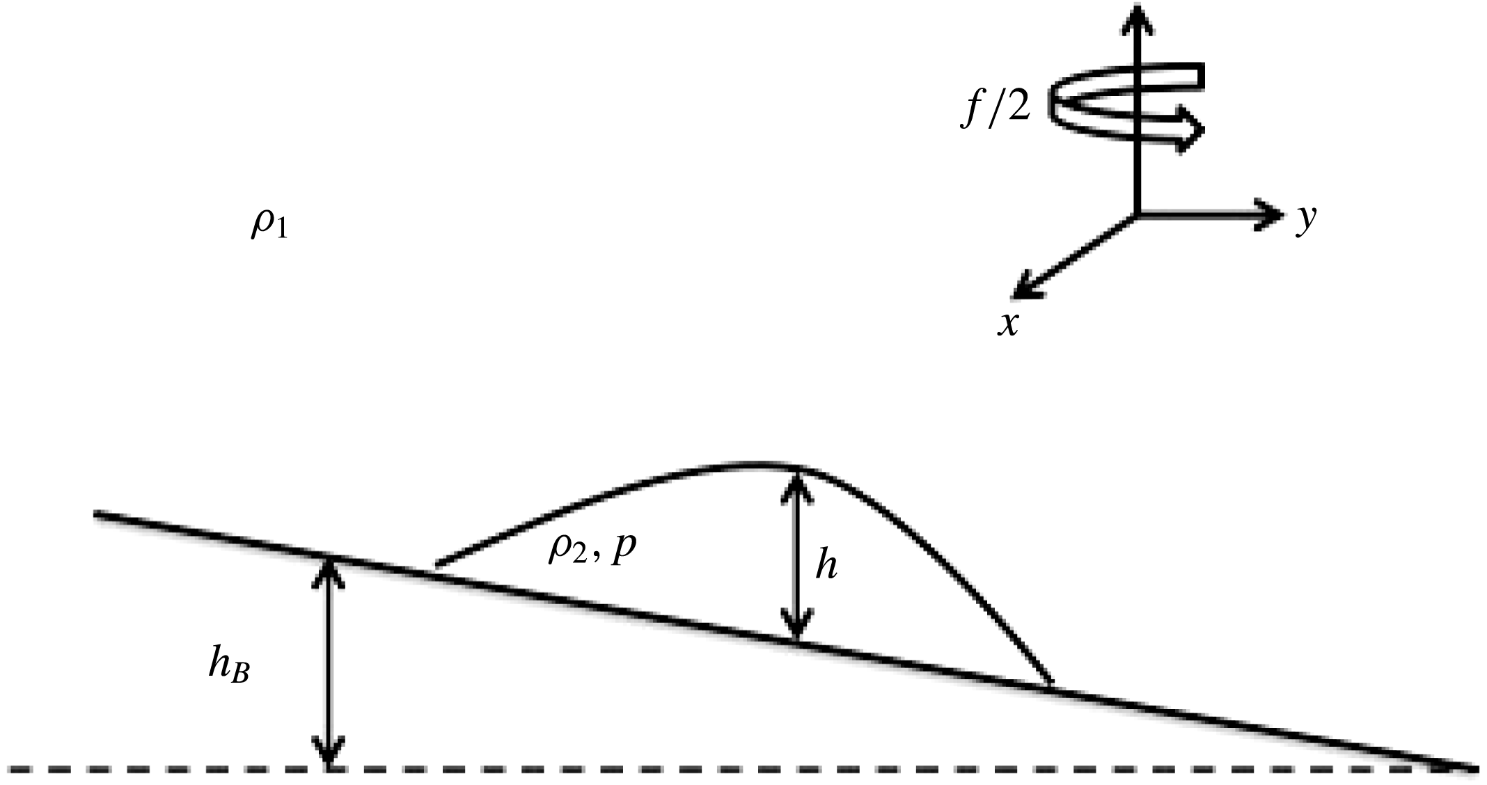
In standard notation (e.g. Pedlosky Reference Pedlosky1987), the dimensional planetary geostrophic reduced-gravity equations describing grounded abyssal flow (see figure 1) over variable topography on a mid-latitude
 $\unicode[STIX]{x1D6FD}$
-plane are given by
 $$\begin{eqnarray}\displaystyle & (f_{0}+\unicode[STIX]{x1D6FD}^{\ast }y)v=g^{\prime }(h+h_{B})_{x}, & \displaystyle\end{eqnarray}$$
 $$\begin{eqnarray}\displaystyle & (f_{0}+\unicode[STIX]{x1D6FD}^{\ast }y)u=-g^{\prime }(h+h_{B})_{y}, & \displaystyle\end{eqnarray}$$
 $$\begin{eqnarray}\displaystyle & h_{t}+\unicode[STIX]{x1D735}\boldsymbol{\cdot }(\boldsymbol{u}h)=0, & \displaystyle\end{eqnarray}$$
where
 $\boldsymbol{u}=(u,v)$
with
 $u$
and
 $v$
the eastward or zonal and northward or meridional velocities, respectively,
 $\unicode[STIX]{x1D735}=(\unicode[STIX]{x2202}_{x},\unicode[STIX]{x2202}_{y})$
with
 $x$
and
 $y$
the eastward and northward coordinates, respectively,
 $f=f_{0}+\unicode[STIX]{x1D6FD}^{\ast }y$
is the meridionally varying Coriolis parameter,
 $h(x,y,t)\geqslant 0$
is the thickness or height of the abyssal water above the bottom topography
 $h_{B}=h_{B}(x,y)$
,
 $g^{\prime }=g(\unicode[STIX]{x1D70C}_{2}-\unicode[STIX]{x1D70C}_{1})/\unicode[STIX]{x1D70C}_{2}>0$
is the stably stratified reduced gravity (where
 $g$
is the gravitational acceleration,
 $\unicode[STIX]{x1D70C}_{1}$
and
 $\unicode[STIX]{x1D70C}_{2}$
are the densities in the overlying water column and within the abyssal water mass, respectively), and
 $t$
is time. The geostrophic pressure in the abyssal water mass is given by
 $p=g^{\prime }\unicode[STIX]{x1D70C}_{2}(h+h_{B})$
and it is assumed, consistent with the reduced-gravity dynamics, that the overlying water column is infinitely deep and motionless.
Geometry of the reduced-gravity model used in this paper. The features are not shown to scale in order to facilitate their description.

It is convenient to non-dimensionalize these equations by introducing the non-dimensional tilde variables
 $$\begin{eqnarray}(x,y)=L(\,\widetilde{x},\widetilde{y}),\quad (u,v)=U_{\ast }(\,\widetilde{u},\widetilde{v}),\quad t=(L/U_{\ast })\widetilde{t},\quad (h,h_{B},p)=s_{\ast }L(\,\widetilde{h},\widetilde{h}_{B},g^{\prime }\unicode[STIX]{x1D70C}_{2}\widetilde{p}),\end{eqnarray}$$
where
 $U_{\ast }=g^{\prime }s_{\ast }/f_{0}$
is the Nof speed (Nof Reference Nof1983),
 $L$
is the horizontal length scale, and
 $s_{\ast }$
is representative of the bottom slope
 $|\unicode[STIX]{x1D735}h_{B}|$
. The Nof speed is the speed of propagation of a steadily travelling compactly supported grounded abyssal water mass on a constant sloping bottom on an
 $f$
-plane as determined by the full nonlinear reduced-gravity shallow-water equations. Substitution of (2.4) into (2.1)–(2.3) leads to, after dropping the tildes,
 $$\begin{eqnarray}\displaystyle & (1+\unicode[STIX]{x1D6FD}y)v=(h+h_{B})_{x}, & \displaystyle\end{eqnarray}$$
 $$\begin{eqnarray}\displaystyle & (1+\unicode[STIX]{x1D6FD}y)u=-(h+h_{B})_{y}, & \displaystyle\end{eqnarray}$$
 $$\begin{eqnarray}\displaystyle & h_{t}+\unicode[STIX]{x1D735}\boldsymbol{\cdot }[(u,v)h]=0, & \displaystyle\end{eqnarray}$$
where
 $\unicode[STIX]{x1D6FD}=\unicode[STIX]{x1D6FD}^{\ast }L/f_{0}$
is the non-dimensional beta parameter and the geostrophic pressure is
 $p=h+h_{B}$
.
Oceanographic estimates, appropriate for the mid-latitude North Atlantic continental slope, are
 $g^{\prime }\simeq 10^{-3}~\text{m}~\text{s}^{-2}$
,
 $s_{\ast }\simeq 5.6\times 10^{-3}$
and
 $L\simeq 100~\text{km}$
(see the discussion in Swaters (Reference Swaters2006a
,Reference Swaters
b
)), suggesting that
 $U_{\ast }\simeq 4~\text{cm}~\text{s}^{-1}$
,
 $\unicode[STIX]{x1D6FD}\simeq 0.02$
, a time scale of
 $T\equiv L/U_{\ast }\simeq 30$
days and an abyssal layer scale thickness of
 $s_{\ast }L\simeq 560~\text{m}$
. Regardless of the magnitude of
 $\unicode[STIX]{x1D6FD}$
, it cannot be neglected over the meridional basin length scales in which we are interested. The value of the slope parameter
 $s_{\ast }$
adopted here has been obtained by averaging US Navy bathymetric data for the continental slope along the east coast of North America from
 $20^{\circ }$
N to
 $60^{\circ }$
N (for full details see Swaters (Reference Swaters2006b
)).
Substitution of (2.5) and (2.6) into (2.7) leads to the quasi-linear hyperbolic partial differential equation
 $$\begin{eqnarray}h_{t}+\text{J}\left(h+h_{B},\frac{h}{1+\unicode[STIX]{x1D6FD}y}\right)=0,\end{eqnarray}$$
where the Jacobian
 $\text{J}(A,B)\equiv A_{x}B_{y}-A_{y}B_{x}$
. Alternatively, (2.8) can be expanded into the form
 $$\begin{eqnarray}h_{t}-\left[\frac{\unicode[STIX]{x1D6FD}h}{(1+\unicode[STIX]{x1D6FD}y)^{2}}+\frac{\unicode[STIX]{x2202}_{y}h_{B}}{1+\unicode[STIX]{x1D6FD}y}\right]h_{x}+\frac{(\unicode[STIX]{x2202}_{x}h_{B})h_{y}}{1+\unicode[STIX]{x1D6FD}y}=\frac{\unicode[STIX]{x1D6FD}(\unicode[STIX]{x2202}_{x}h_{B})h}{(1+\unicode[STIX]{x1D6FD}y)^{2}}.\end{eqnarray}$$
The potential vorticity (PV) equation associated with this model is simply obtained by multiplying (2.8) with
 $(1+\unicode[STIX]{x1D6FD}y)^{-1}$
, yielding
 $$\begin{eqnarray}\left(\frac{h}{1+\unicode[STIX]{x1D6FD}y}\right)_{t}+\boldsymbol{u}\boldsymbol{\cdot }\unicode[STIX]{x1D735}\left(\frac{h}{1+\unicode[STIX]{x1D6FD}y}\right)=0,\end{eqnarray}$$
where (2.5) and (2.6) have been used. Equation (2.9) may be interpreted as a variant of the so-called planetary geostrophic wave equation introduced by Anderson & Killworth (Reference Anderson and Killworth1979), Dewar (Reference Dewar1987), Wright & Willmott (Reference Wright and Willmott1992) and Edwards, Willmott & Killworth (Reference Edwards, Willmott and Killworth1998), generalized to allow for meridional flow on a mid-latitude
 $\unicode[STIX]{x1D6FD}$
-plane with variable bottom topography. The model equation (2.8) possesses a non-canonical Hamiltonian formulation (Swaters Reference Swaters2018).
One useful property of the model (2.9) is that it ensures that the appropriate kinematic condition associated with a grounding (i.e. a location where
 $h$
intersects the bottom; as an example see figure 1) is automatically satisfied. That is, one does not need to apply the kinematic boundary condition as an additional auxiliary external constraint since the solution to (2.9) will necessarily automatically satisfy it. To see this, suppose that a grounding occurs along the potentially time-dependent curve
 $y=\widetilde{y}(x,t)$
, i.e.
 $h(x,\widetilde{y}(x,t),t)=0$
. The appropriate kinematic boundary condition can be written in the form
 $$\begin{eqnarray}[\unicode[STIX]{x2202}_{t}+(u,v)\cdot (\unicode[STIX]{x2202}_{x},\unicode[STIX]{x2202}_{y})][y-\widetilde{y}(x,t)]=0\quad \text{evaluated on }y=\widetilde{y}(x,t),\end{eqnarray}$$
which reduces to
 $$\begin{eqnarray}-\widetilde{y}_{t}+v-u\widetilde{y}_{x}=0\quad \text{evaluated on }y=\widetilde{y}(x,t).\end{eqnarray}$$
However, it follows from
 $h(x,\widetilde{y}(x,t),t)=0$
that
 $$\begin{eqnarray}h_{t}+h_{y}\widetilde{y}_{t}=0\quad \text{evaluated on }y=\widetilde{y}(x,t),\end{eqnarray}$$
and
 $$\begin{eqnarray}h_{x}+h_{y}\widetilde{y}_{x}=0\quad \text{evaluated on }y=\widetilde{y}(x,t),\end{eqnarray}$$
which when substituted into (2.12) implies
 $$\begin{eqnarray}\frac{h_{t}}{h_{y}}+\frac{(h+h_{B})_{x}}{1+\unicode[STIX]{x1D6FD}y}-\frac{(h+h_{B})_{y}h_{x}}{(1+\unicode[STIX]{x1D6FD}y)\,h_{y}}=0\quad \text{evaluated on }y=\widetilde{y}(x,t),\end{eqnarray}$$
which simplifies to
 $$\begin{eqnarray}h_{t}+\frac{(\unicode[STIX]{x2202}_{x}h_{B})h_{y}}{1+\unicode[STIX]{x1D6FD}y}-\frac{(\unicode[STIX]{x2202}_{y}h_{B})h_{x}}{1+\unicode[STIX]{x1D6FD}y}=0\quad \text{evaluated on }y=\widetilde{y}(x,t).\end{eqnarray}$$
But this latter equation is identical to (2.9) evaluated on the grounding
 $y=\widetilde{y}(x,t)$
. Thus, no additional boundary conditions are needed to ensure that the solution of (2.9) will satisfy the appropriate kinematic boundary condition on a grounding. This property is very convenient when constructing numerical solutions.
3 Steady solution
The steady or time-independent solutions of (2.9) satisfy the quasi-linear hyperbolic equation
 $$\begin{eqnarray}(1+\unicode[STIX]{x1D6FD}y)(\unicode[STIX]{x2202}_{x}h_{B})h_{y}-[\unicode[STIX]{x1D6FD}h+(1+\unicode[STIX]{x1D6FD}y)(\unicode[STIX]{x2202}_{y}h_{B})]h_{x}=\unicode[STIX]{x1D6FD}(\unicode[STIX]{x2202}_{x}h_{B})h,\end{eqnarray}$$
which can be solved exactly for arbitrary bottom topography
 $h_{B}(x,y)$
using the method of characteristics (for details in the spherical coordinate context when
 $h_{B}$
is assumed to vary only in the longitudinal direction, see Swaters (Reference Swaters2013)). If, along
 $y=y_{0}$
, we suppose that
 $h_{B}(x,y_{0})=h_{B0}(x)$
and that
 $h(x,y_{0})=h_{0}(x)$
, then the solution to (3.1) can be written in the form
 $$\begin{eqnarray}\displaystyle & \displaystyle h(x,y)=\frac{1+\unicode[STIX]{x1D6FD}y}{1+\unicode[STIX]{x1D6FD}y_{0}}h_{0}(\unicode[STIX]{x1D70F}), & \displaystyle\end{eqnarray}$$
 $$\begin{eqnarray}\displaystyle & \displaystyle h_{B}(x,y)=\frac{\unicode[STIX]{x1D6FD}(y_{0}-y)}{1+\unicode[STIX]{x1D6FD}y_{0}}h_{0}(\unicode[STIX]{x1D70F})+h_{B0}(\unicode[STIX]{x1D70F}), & \displaystyle\end{eqnarray}$$
where
 $\unicode[STIX]{x1D70F}=x$
on
 $y=y_{0}$
. General steady solutions to (3.1) satisfy the first-order necessary conditions for an extremum to a suitably constrained energy functional (Swaters Reference Swaters2018).
The characteristics, which are the isolines in the
 $(x,y)$
plane for constant
 $\unicode[STIX]{x1D70F}$
, are also the geostrophic streamlines since (3.2) and (3.3) can be combined to yield
 $$\begin{eqnarray}h(x,y)+h_{B}(x,y)=h_{0}(\unicode[STIX]{x1D70F})+h_{B0}(\unicode[STIX]{x1D70F}),\end{eqnarray}$$
since
 $h(x,y)+h_{B}(x,y)$
is the geostrophic pressure. In practice, one determines
 $\unicode[STIX]{x1D70F}(x,y)$
from (3.3) and substitutes into (3.2) to determine
 $h(x,y)$
. Once
 $h$
is known, the velocities are determined by the geostrophic relations (2.5) and (2.6). Thus, given knowledge of the cross-slope structure or shape of the abyssal water mass height
 $h$
at the northern boundary of a region in the northern hemisphere (or southern boundary in the case of the southern hemisphere), equations (3.2) and (3.3) determine the steady equatorward flow equatorward of the location of the boundary condition.
The solution (3.2) and (3.3) is not a parallel shear flow and is one of the few known exact nonlinear solutions for steady flow that crosses the planetary vorticity gradient. Qualitatively, the solution has the property that
 $h$
decreases and the flow speeds up (while maintaining constant meridional volume transport; see Swaters (Reference Swaters2015a
)) and has a slight upslope trajectory as the flow moves equatorward (consistent with primitive equation simulations, e.g. Spall (Reference Spall1994), or shallow-water simulations, e.g. Kim et al. (Reference Kim, Swaters and Sutherland2014), and observations, e.g. Fischer & Schott (Reference Fischer and Schott1997), Joyce et al. (Reference Joyce, Dunworth-Baker, Pickart and Waterman2005), Cunningham et al. (Reference Cunningham, Kanzow, Rayner, Baringer, Johns, Marotzke, Longworth, Grant, Hirschi and Beal2007)). There is very good pointwise agreement between this steady solution and the time-averaged mid-latitude height and velocity fields associated with the fully nonlinear shallow-water initial-value numerical simulations (see the discussion in Kim et al. (Reference Kim, Swaters and Sutherland2014)). We will illustrate the solution with a simple example later in this section.
The only ‘disorder’ that can occur in the solution (3.2) and (3.3) is the possible emergence of a shock (as a consequence of the quasi-linearity in (3.1)). The shock will form at the first
 $y$
-value equatorward of
 $y_{0}$
for which
 $|h_{x}|\rightarrow \infty$
. It follows from (3.2) and (3.3) that
 $$\begin{eqnarray}h_{x}=\frac{(1+\unicode[STIX]{x1D6FD}y)h_{0}^{\prime }(\unicode[STIX]{x1D70F})(\unicode[STIX]{x2202}_{x}h_{B})}{(1+\unicode[STIX]{x1D6FD}y_{0})h_{B0}^{\prime }(\unicode[STIX]{x1D70F})+\unicode[STIX]{x1D6FD}(y_{0}-y)h_{0}^{\prime }(\unicode[STIX]{x1D70F})},\end{eqnarray}$$
so that
 $|h_{x}|\rightarrow \infty$
for
 $y=y_{s}$
given by
 $$\begin{eqnarray}\frac{1+\unicode[STIX]{x1D6FD}y_{s}}{1+\unicode[STIX]{x1D6FD}y_{0}}=\frac{h_{B0}^{\prime }(\unicode[STIX]{x1D70F})+h_{0}^{\prime }(\unicode[STIX]{x1D70F})}{h_{0}^{\prime }(\unicode[STIX]{x1D70F})}.\end{eqnarray}$$
Let us focus on the northern hemisphere for concreteness of argument (the extension to the southern hemisphere will follow straightforwardly provided the appropriate non-dimensionalization is taken into account). Since we are implicitly modelling equatorward flow along the western side of an ocean basin, we assume the bottom slope along
 $y=y_{0}$
satisfies
 $h_{B0}^{\prime }(\unicode[STIX]{x1D70F})<0$
(i.e. the bottom topography deepens as one moves eastward). In addition, in accordance with the underlying assumptions of the
 $\unicode[STIX]{x1D6FD}$
-plane approximation,
 $$\begin{eqnarray}0<\frac{1+\unicode[STIX]{x1D6FD}y_{s}}{1+\unicode[STIX]{x1D6FD}y_{0}}\leqslant 1\quad \text{for }-\unicode[STIX]{x1D6FD}^{-1}\ll y_{s}\leqslant y_{0},\end{eqnarray}$$
for equatorward flow in the northern hemisphere. It follows, therefore, that a shock can only occur if there are
 $\unicode[STIX]{x1D70F}$
values for which
 $h_{0}^{\prime }(\unicode[STIX]{x1D70F})>0$
since if
 $h_{0}^{\prime }(\unicode[STIX]{x1D70F})<0$
then (3.6) would imply that
 $y_{s}>y_{0}$
, which is poleward of
 $y_{0}$
and thus outside our region of interest. Thus, a shock can only form in the region
 $y_{s}\leqslant y_{0}$
if there are
 $\unicode[STIX]{x1D70F}$
values for which
 $$\begin{eqnarray}0<\frac{h_{B0}^{\prime }(\unicode[STIX]{x1D70F})+h_{0}^{\prime }(\unicode[STIX]{x1D70F})}{h_{0}^{\prime }(\unicode[STIX]{x1D70F})}\leqslant 1\quad \text{and}\quad h_{0}^{\prime }(\unicode[STIX]{x1D70F})>0\quad \Longrightarrow \quad h_{B0}^{\prime }(\unicode[STIX]{x1D70F})+h_{0}^{\prime }(\unicode[STIX]{x1D70F})>0.\end{eqnarray}$$
Consequently, should it be the case that
 $$\begin{eqnarray}h_{B0}^{\prime }(\unicode[STIX]{x1D70F})+h_{0}^{\prime }(\unicode[STIX]{x1D70F})<0\quad \text{for all }\unicode[STIX]{x1D70F},\end{eqnarray}$$
then no shock can form in the region
 $-\unicode[STIX]{x1D6FD}^{-1}\ll y\leqslant y_{0}$
.
Condition (3.9) has a straightforward physical interpretation. The meridional velocity
 $v(x,y_{0})$
is given by
 $$\begin{eqnarray}v(x,y_{0})=\frac{h^{\prime }(x)+h_{B0}^{\prime }(x)}{1+\unicode[STIX]{x1D6FD}y_{0}}.\end{eqnarray}$$
Thus, if the meridional velocity within the abyssal water mass along the boundary
 $y=y_{0}$
is everywhere equatorward, no shock forms in the solution (3.2) and (3.3) in the region equatorward of
 $y=y_{0}$
. Of course, the argument presented here applies only to a mid-latitude
 $\unicode[STIX]{x1D6FD}$
-plane or on a sphere that does not extend to the equator. On an equatorial
 $\unicode[STIX]{x1D6FD}$
-plane, the analogues of these solutions for the geostrophic velocities ultimately become singular as the equator is approached regardless of the flow profile along the poleward boundary of the region (Swaters Reference Swaters2013, Reference Swaters2015a
) and new dynamics must prevail in the equatorial region (Swaters Reference Swaters2015b
). We hasten to add that in light of the no-shock condition (3.9) the configuration shown in figure 1 corresponds to a cross-slope abyssal height profile which would in fact develop a shock. The abyssal height profile in figure 1 has been exaggerated in order to clearly show the geometry and relevant variables.
3.1 A simple example
As a very simple example for which it is possible to write down an explicit solution (Swaters (Reference Swaters2013, Reference Swaters2015a
) describes the nonlinear steady solution associated with a boundary abyssal height profile
 $h(x,y_{0})$
that possesses both upslope and downslope groundings) let us consider the case for which
 $$\begin{eqnarray}h_{B}=-x\quad \text{and}\quad h_{0}(x)=\widetilde{h}_{0}-\unicode[STIX]{x1D6FC}x,\end{eqnarray}$$
where
 $\widetilde{h}_{0}>0$
and
 $\unicode[STIX]{x1D6FC}$
are constants. In this simple example, the bottom topography has constant slope and the water column deepens as
 $x$
increases. The abyssal water mass height along
 $y=y_{0}$
varies linearly in the cross-slope direction and has a single grounding located at
 $x=x_{g}\equiv \widetilde{h}_{0}/\unicode[STIX]{x1D6FC}$
, and the meridional velocity along
 $y=y_{0}$
is
 $v(x,y_{0})=-(1+\unicode[STIX]{x1D6FC})$
, which is independent of
 $x$
. There is no loss of generality in choosing
 $h_{B}^{\prime }=-1$
on account of the underlying non-dimensionalization scheme in (2.4). (Observe that if
 $\unicode[STIX]{x1D6FC}=-1$
then
 $h_{B}+h_{0}=\widetilde{h}_{0}$
, implying
 $v=0$
along
 $y=y_{0}$
.) The no-shock condition (3.9), in this example, reduces to simply
 $$\begin{eqnarray}1+\unicode[STIX]{x1D6FC}>0.\end{eqnarray}$$
Substitution of (3.11) into (3.3) implies that the characteristics or geostrophic streamlines are the non-parallel lines given by (for constant
 $\unicode[STIX]{x1D70F}$
)
 $$\begin{eqnarray}\unicode[STIX]{x1D70F}(x,y)=\frac{x(1+\unicode[STIX]{x1D6FD}y_{0})+\unicode[STIX]{x1D6FD}\widetilde{h}_{0}(y_{0}-y)}{1+\unicode[STIX]{x1D6FD}y_{0}+\unicode[STIX]{x1D6FC}\unicode[STIX]{x1D6FD}(y_{0}-y)},\end{eqnarray}$$
which if substituted into (3.2) yields
 $$\begin{eqnarray}h(x,y)=\frac{(1+\unicode[STIX]{x1D6FD}y)(\,\widetilde{h}_{0}-\unicode[STIX]{x1D6FC}x)}{1+\unicode[STIX]{x1D6FD}y_{0}+\unicode[STIX]{x1D6FC}\unicode[STIX]{x1D6FD}(y_{0}-y)},\end{eqnarray}$$
from which we see, of course, that
 $\unicode[STIX]{x1D70F}(x,y_{0})=x$
and
 $h(x,y_{0})=h_{0}(x)$
. It is only for this simple example that the solution for
 $h(x,y)$
has the separated form seen in (3.14) with respect to its
 $x$
and
 $y$
dependences. In general, it does not (see Swaters Reference Swaters2013, Reference Swaters2015a
).
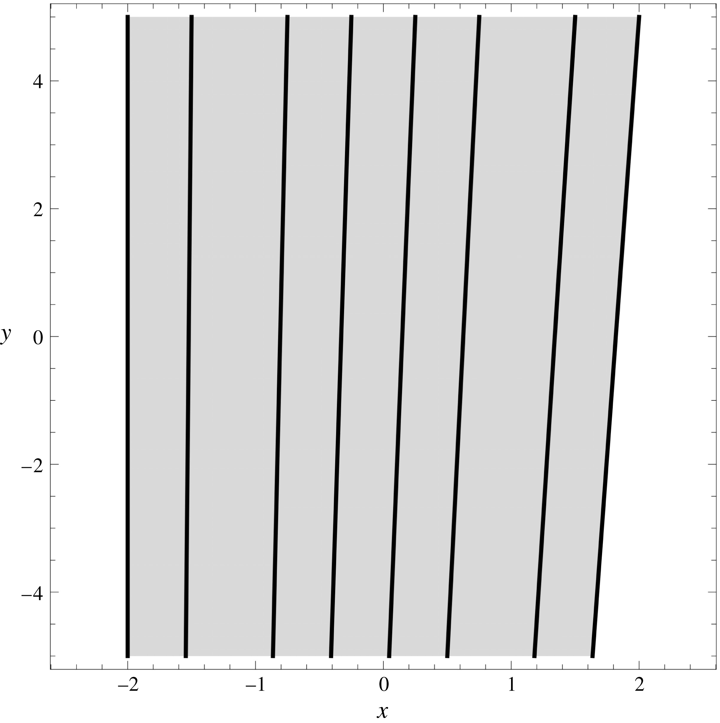
Figure 2 is a contour plot of the characteristics or geostrophic streamlines
 $\unicode[STIX]{x1D70F}(x,y)$
as given by (3.13) for the parameter values
 $\widetilde{h}_{0}=1$
,
 $\unicode[STIX]{x1D6FD}=0.02$
,
 $y_{0}=5$
and
 $\unicode[STIX]{x1D6FC}=-0.5$
(corresponding to an equatorward speed of approximately
 $2~\text{cm}~\text{s}^{-1}$
) for the region
 $-2\leqslant x\leqslant 2.5$
and
 $-5\leqslant y\leqslant 5$
for the selected contours
 $\unicode[STIX]{x1D70F}=-2.0$
,
 $-1.5$
,
 $-0.75$
, 0.0, 0.5, 1.25 and 2.0, respectively. The shaded region corresponds to where
 $h(x,y)>0$
. The flow is grounded along
 $x=x_{g}=-2.0$
and
 $h(x,y)>0$
for
 $x>-2.0$
. Other than the
 $\unicode[STIX]{x1D70F}=-2.0$
contour, all the other contours possess the property that
 $\text{d}y/\text{d}x>0$
for fixed
 $\unicode[STIX]{x1D70F}$
, implying a slight upslope velocity as the flow moves equatorward.
Contour plot of the geostrophic streamlines
 $\unicode[STIX]{x1D70F}(x,y)$
for selected
 $\unicode[STIX]{x1D70F}$
contours.

Note that it follows from (3.14) that the location of the grounding is constant with respect to
 $y$
. This is a general result independent of the boundary condition (see Swaters Reference Swaters2013, Reference Swaters2015a
) that requires only that the topography be independent of
 $y$
.
The meridional velocity
 $v$
associated with this simple example is independent of
 $x$
and is given by
 $$\begin{eqnarray}v=\frac{(h_{B}+h)_{x}}{1+\unicode[STIX]{x1D6FD}y}=-\frac{(1+\unicode[STIX]{x1D6FC})(1+\unicode[STIX]{x1D6FD}y_{0})}{(1+\unicode[STIX]{x1D6FD}y)[1+\unicode[STIX]{x1D6FD}y_{0}+\unicode[STIX]{x1D6FC}\unicode[STIX]{x1D6FD}(y_{0}-y)]}<0,\end{eqnarray}$$
for the region
 $-\unicode[STIX]{x1D6FD}^{-1}\ll y\leqslant y_{0}$
(focusing on the northern hemisphere). It follows from (3.15) that
 $v_{y}<0$
in this example. The increase in the equatorward speed is exactly compensated for by the decreasing height
 $h$
as
 $y$
moves equatorward so that the meridional volume transport is constant with respect to
 $y$
(see Swaters Reference Swaters2013, Reference Swaters2015a
). For example, if we denote the equatorward transport between the
 $\unicode[STIX]{x1D70F}=-2.0$
and
 $\unicode[STIX]{x1D70F}=3.0$
geostrophic streamlines as
 $T$
, it follows after a little algebra that
 $$\begin{eqnarray}T\equiv \int _{x_{g}}^{x_{\unicode[STIX]{x1D70F}=3}}v(x,y)h(x,y)\,\text{d}x=\frac{(1+\unicode[STIX]{x1D6FC})(\,\widetilde{h}_{0}-3\unicode[STIX]{x1D6FC})^{2}}{2\unicode[STIX]{x1D6FC}(1+\unicode[STIX]{x1D6FD}y_{0})}<0,\end{eqnarray}$$
for this example.
The zonal velocity
 $u$
associated with this simple example is given by
 $$\begin{eqnarray}u(x,y)=-\frac{h_{y}}{1+\unicode[STIX]{x1D6FD}y}=-\frac{\unicode[STIX]{x1D6FD}(1+\unicode[STIX]{x1D6FC})(1+\unicode[STIX]{x1D6FD}y_{0})(\,\widetilde{h}_{0}-\unicode[STIX]{x1D6FC}x)}{(1+\unicode[STIX]{x1D6FD}y)[1+\unicode[STIX]{x1D6FD}y_{0}+\unicode[STIX]{x1D6FC}\unicode[STIX]{x1D6FD}(y_{0}-y)]^{2}}<0,\end{eqnarray}$$
so that there is a
 $O(\unicode[STIX]{x1D6FD})$
upslope or westward velocity as the flow moves equatorward that is induced by the planetary vorticity gradient.
4 Initial-value solution
Let us consider the initial-value (or Cauchy) problem for which
 $$\begin{eqnarray}h(x,y,0)=h_{0}(x,y),\end{eqnarray}$$
where
 $h_{0}(x,y)$
is a given initial abyssal height profile. The characteristic equations associated with (2.9) for the initial-value problem can be written in the form
 $$\begin{eqnarray}\displaystyle & \displaystyle \frac{\text{d}t}{\text{d}s}=1\quad \text{with }t|_{s=0}=0, & \displaystyle\end{eqnarray}$$
 $$\begin{eqnarray}\displaystyle & \displaystyle \frac{\text{d}x}{\text{d}s}=-\frac{\unicode[STIX]{x1D6FD}h}{(1+\unicode[STIX]{x1D6FD}y)^{2}}-\frac{\unicode[STIX]{x2202}_{y}h_{B}}{1+\unicode[STIX]{x1D6FD}y}\quad \text{with }x|_{s=0}=\unicode[STIX]{x1D707}, & \displaystyle\end{eqnarray}$$
 $$\begin{eqnarray}\displaystyle & \displaystyle \frac{\text{d}y}{\text{d}s}=\frac{\unicode[STIX]{x2202}_{x}h_{B}}{1+\unicode[STIX]{x1D6FD}y}\quad \text{with }y|_{s=0}=\unicode[STIX]{x1D702}, & \displaystyle\end{eqnarray}$$
 $$\begin{eqnarray}\displaystyle & \displaystyle \frac{\text{d}h}{\text{d}s}=\frac{\unicode[STIX]{x1D6FD}(\unicode[STIX]{x2202}_{x}h_{B})h}{(1+\unicode[STIX]{x1D6FD}y)^{2}}\quad \text{with }h|_{s=0}=h_{0}(\unicode[STIX]{x1D707},\unicode[STIX]{x1D702}), & \displaystyle\end{eqnarray}$$
where
 $s$
is the characteristic coordinate ‘along’ the characteristics and
 $h_{0}(\unicode[STIX]{x1D707},\unicode[STIX]{x1D702})$
is parametrized in terms of
 $\unicode[STIX]{x1D707}$
and
 $\unicode[STIX]{x1D702}$
, the characteristic coordinates associated with
 $x$
and
 $y$
, respectively.
Three immediate integrations are possible. It follows from (4.2) that
 $$\begin{eqnarray}t=s.\end{eqnarray}$$
From (4.4) and (4.5) one obtains
 $$\begin{eqnarray}h=\frac{1+\unicode[STIX]{x1D6FD}y}{1+\unicode[STIX]{x1D6FD}\unicode[STIX]{x1D702}}h_{0}(\unicode[STIX]{x1D707},\unicode[STIX]{x1D702}).\end{eqnarray}$$
It follows from (4.3)–(4.5) that
 $$\begin{eqnarray}\frac{\text{d}h_{B}}{\text{d}s}=(\unicode[STIX]{x2202}_{x}h_{B})\frac{\text{d}x}{\text{d}s}+(\unicode[STIX]{x2202}_{y}h_{B})\frac{\text{d}y}{\text{d}s}=-\frac{\text{d}h}{\text{d}s},\end{eqnarray}$$
which can be integrated to yield
 $$\begin{eqnarray}h+h_{B}(x,y)=h_{0}(\unicode[STIX]{x1D707},\unicode[STIX]{x1D702})+h_{B}(\unicode[STIX]{x1D707},\unicode[STIX]{x1D702}).\end{eqnarray}$$
Equations (4.7) and (4.9) can be combined to give
 $$\begin{eqnarray}h_{B}(x,y)=\frac{\unicode[STIX]{x1D6FD}(\unicode[STIX]{x1D702}-y)}{1+\unicode[STIX]{x1D6FD}\unicode[STIX]{x1D702}}h_{0}(\unicode[STIX]{x1D707},\unicode[STIX]{x1D702})+h_{B}(\unicode[STIX]{x1D707},\unicode[STIX]{x1D702}),\end{eqnarray}$$
which is the analogue of (3.3) for the initial-value problem. This is as far as one can go analytically for general topography. In general, one must numerically solve (4.3) and (4.4) to find an additional relationship connecting
 $(x,y)$
and
 $(\unicode[STIX]{x1D707},\unicode[STIX]{x1D702})$
, which will then complete the solution. However, for a linearly sloping bottom, further analytical progress is possible.
4.1 Linearly sloping bottom
In the approximation that
 $$\begin{eqnarray}h_{B}=-x,\end{eqnarray}$$
the nonlinear solution to the initial-value problem, although implicit, can be completely determined. Assuming (4.11), it follows from (4.4) and (4.6) that
 $$\begin{eqnarray}\unicode[STIX]{x1D702}(y,t)=\frac{-1+\sqrt{(1+\unicode[STIX]{x1D6FD}y)^{2}+2\unicode[STIX]{x1D6FD}t}}{\unicode[STIX]{x1D6FD}},\end{eqnarray}$$
which when substituted into (4.10) yields
 $$\begin{eqnarray}x=\unicode[STIX]{x1D707}+\frac{\left[1+\unicode[STIX]{x1D6FD}y-\sqrt{(1+\unicode[STIX]{x1D6FD}y)^{2}+2\unicode[STIX]{x1D6FD}t}\right]}{\sqrt{(1+\unicode[STIX]{x1D6FD}y)^{2}+2\unicode[STIX]{x1D6FD}t}}\,h_{0}\left(\unicode[STIX]{x1D707},\frac{-1+\sqrt{(1+\unicode[STIX]{x1D6FD}y)^{2}+2\unicode[STIX]{x1D6FD}t}}{\unicode[STIX]{x1D6FD}}\right).\end{eqnarray}$$
We note that the initial conditions associated with the characteristic equations imply that
 $\unicode[STIX]{x1D702}(y,0)=y$
and
 $\unicode[STIX]{x1D707}(x,y,0)=x$
. Thus, given
 $(x,y,t)$
,
 $\unicode[STIX]{x1D702}$
is determined by (4.12) and
 $\unicode[STIX]{x1D707}$
implicitly by (4.13), and consequently
 $h(x,y,t)$
by (4.7). We now turn to two illustrative examples where a complete analytical description is possible.
4.2 Initial parallel along-slope flow with no cross-slope shear
As a very simple initial-value example for which it is possible to write down an explicit nonlinear time-dependent solution, let us consider the initial conditions
 $$\begin{eqnarray}h_{B}=-x\quad \text{and}\quad h_{0}(x,y)=\widetilde{h}_{0}-\unicode[STIX]{x1D6FC}x,\end{eqnarray}$$
with
 $1+\unicode[STIX]{x1D6FC}>0$
(no-shock condition), corresponding to an initial parallel along-slope equatorward flow with no cross-slope shear in the along-slope velocity. Substitution of (4.14) into (4.13) implies
 $$\begin{eqnarray}\unicode[STIX]{x1D707}=\frac{(\,\widetilde{h}_{0}+x)\sqrt{(1+\unicode[STIX]{x1D6FD}y)^{2}+2\unicode[STIX]{x1D6FD}t}-\widetilde{h}_{0}(1+\unicode[STIX]{x1D6FD}y)}{(1+\unicode[STIX]{x1D6FC})\sqrt{(1+\unicode[STIX]{x1D6FD}y)^{2}+2\unicode[STIX]{x1D6FD}t}-\unicode[STIX]{x1D6FC}(1+\unicode[STIX]{x1D6FD}y)},\end{eqnarray}$$
which if substituted into (4.7) yields the explicit nonlinear time-dependent solution for the abyssal height given by
 $$\begin{eqnarray}h(x,y,t)=\frac{(\,\widetilde{h}_{0}-\unicode[STIX]{x1D6FC}x)(1+\unicode[STIX]{x1D6FD}y)}{(1+\unicode[STIX]{x1D6FC})\sqrt{(1+\unicode[STIX]{x1D6FD}y)^{2}+2\unicode[STIX]{x1D6FD}t}-\unicode[STIX]{x1D6FC}(1+\unicode[STIX]{x1D6FD}y)}.\end{eqnarray}$$
Similar to the steady solution (3.14), it is only for this very simple example that the solution for
 $h(x,y,t)$
has the separated form with respect to its
 $x$
and
 $(y,t)$
dependences, respectively. In general, it will not. The no-shock condition
 $1+\unicode[STIX]{x1D6FC}>0$
ensures that the denominator in (4.16) is never zero for any
 $t\geqslant 0$
.
The solution (4.16) describes a time-dependent flow that evolves away from a parallel along-slope flow with no cross-slope shear. The abyssal current height is non-zero only for
 $x>\widetilde{h}_{0}/\unicode[STIX]{x1D6FC}=-2.0$
(i.e. there is a grounding along
 $x=\widetilde{h}_{0}/\unicode[STIX]{x1D6FC}$
which does not change in time (see Swaters Reference Swaters2013, Reference Swaters2015a
)) and there is no abyssal current in the region
 $x<\widetilde{h}_{0}/\unicode[STIX]{x1D6FC}$
. The initial geostrophic pressure contours are parallel to the isobaths.
As
 $t$
increases, the geostrophic pressure contours become oriented in a (time-dependent) southwest-to-northeast configuration as a result of the
 $\unicode[STIX]{x1D6FD}$
-induced upslope deflection of the equatorward flow. Further, as
 $t$
increases, for fixed
 $x$
and
 $y$
,
 $h$
decreases towards zero. The net effect is for
 $(h+h_{B})_{x}$
to decrease. This corresponds to a ‘speeding up’ of the equatorward flow within the abyssal current for fixed
 $x$
and
 $y$
. It follows from (4.4) and (4.14) that the equatorward velocity increases as one moves equatorward. However, from (4.7), given an initial position
 $\unicode[STIX]{x1D707}$
and
 $\unicode[STIX]{x1D702}$
,
 $h$
monotonically decreases as one moves equatorward. Thus, the solution at position
 $(x,y)$
for a given
 $t$
is determined by data located at position
 $(\unicode[STIX]{x1D707},\unicode[STIX]{x1D702})$
at
 $t=0$
, which is necessarily northward of
 $y$
. And since the initial data
 $h_{0}(x,y)$
are independent of
 $y$
, this means that
 $h$
continuously decreases for fixed
 $(x,y)$
as
 $t$
increases.
Although the formal limit
 $t\rightarrow \infty$
is not physically meaningful in the mid-latitude approximation examined here (see the comment made below), one can say that the trend in this solution as time increases, since
 $h$
is decreasing towards zero, is for the geostrophic pressure to approach
 $h_{B}(x)$
. That is, the flow is approaching a parallel along-slope flow in which the cross-slope velocity is zero and the equatorward speed (for fixed
 $y$
) has increased towards
 $1/(1+\unicode[STIX]{x1D6FD}y)$
.
4.3 Initial isolated grounded abyssal dome or pool
As another initial-value example for which it is possible to write down an explicit nonlinear solution, let us consider the case for which
 $h_{B}=-x$
with the initial abyssal height given by
 $$\begin{eqnarray}h_{0}(x,y)=\left\{\begin{array}{@{}ll@{}}\widetilde{h}_{0}\left(1-{\displaystyle \frac{x^{2}+y^{2}}{a^{2}}}\right)\quad & \text{if }x^{2}+y^{2}\leqslant a^{2},\\ 0\quad & \text{if }x^{2}+y^{2}>a^{2},\end{array}\right.\end{eqnarray}$$
(where
 $a>0$
) with
 $0<\widetilde{h}_{0}<a/2$
(this ensures that the initial meridional velocity is everywhere equatorward, which in turn ensures that a shock does not develop in the solution in the region and over the time of interest), corresponding to an isolated abyssal dome or pool centred at
 $x=y=0.0$
with maximum height
 $\widetilde{h}_{0}>0$
. Isolated grounded abyssal domes or pools that survive for months have been observed on, for example, the North American continental slope (e.g. Armi & D’Asaro Reference Armi and D’Asaro1980; Houghton et al.
Reference Houghton, Schlitz, Beardsley, Butman and Chamberlin1982; Ou & Houghton Reference Ou and Houghton1982). Isolated abyssal domes are also seen to emerge in baroclinic instability numerical simulations of unstable grounded abyssal currents (e.g. Swaters Reference Swaters1998). The nonlinear solution we present here is a non-steady meridionally travelling
 $\unicode[STIX]{x1D6FD}$
-plane generalization (within the context of the planetary geostrophic approximation) of the propagating ‘cold eddy’ solution described by Nof (Reference Nof1983). The solution described here is one of the few known exact nonlinear solutions for a propagating coherent isolated eddy that crosses the planetary vorticity gradient.
Substitution of (4.17) into (4.13) implies, after a little algebra, that
 $$\begin{eqnarray}\unicode[STIX]{x1D707}(x,y,t)=\left\{\begin{array}{@{}ll@{}}\unicode[STIX]{x1D6F9}(x,y,t)\quad & \text{if }\unicode[STIX]{x1D6F9}^{2}+\unicode[STIX]{x1D702}^{2}\leqslant a^{2},\\ x\quad & \text{if }\unicode[STIX]{x1D6F9}^{2}+\unicode[STIX]{x1D702}^{2}>a^{2},\end{array}\right.\end{eqnarray}$$
where
 $$\begin{eqnarray}\unicode[STIX]{x1D6F9}(x,y,t)\equiv \frac{2[(\unicode[STIX]{x1D702}^{2}-a^{2})\unicode[STIX]{x1D6E4}+xa^{2}]}{a^{2}+\sqrt{a^{4}-4\unicode[STIX]{x1D6E4}[(\unicode[STIX]{x1D702}^{2}-a^{2})\unicode[STIX]{x1D6E4}+xa^{2}]}},\end{eqnarray}$$
with
 $$\begin{eqnarray}\unicode[STIX]{x1D6E4}(y,t)\equiv \frac{\widetilde{h}_{0}\left[1+\unicode[STIX]{x1D6FD}y-\sqrt{(1+\unicode[STIX]{x1D6FD}y)^{2}+2\unicode[STIX]{x1D6FD}t}\right]}{\sqrt{(1+\unicode[STIX]{x1D6FD}y)^{2}+2\unicode[STIX]{x1D6FD}t}},\end{eqnarray}$$
where
 $\unicode[STIX]{x1D702}(y,t)$
is given by (4.12). Finally, it follows from (4.7) that
 $h(x,y,t)$
will be given by
 $$\begin{eqnarray}h(x,y,t)=\frac{1+\unicode[STIX]{x1D6FD}y}{1+\unicode[STIX]{x1D6FD}\unicode[STIX]{x1D702}(y,t)}\,h_{0}(\unicode[STIX]{x1D707}(x,y,t),\unicode[STIX]{x1D702}(y,t)).\end{eqnarray}$$
We note that the initial conditions associated with the characteristic equations imply
 $\unicode[STIX]{x1D6F9}(x,y,0)=x$
. In addition, note that
 $\unicode[STIX]{x1D6E4}(y,0)=0$
and that
 $\unicode[STIX]{x1D6E4}(y,t)<0$
for
 $t>0$
.
It is important to point out that, since these time-dependent solutions describe equatorward-propagating solutions on a mid-latitude
 $\unicode[STIX]{x1D6FD}$
-plane for which we assume
 $-\unicode[STIX]{x1D6FD}^{-1}\ll y\simeq O(1)$
(focusing on the northern hemisphere), there will be an upper limit in time for which these solutions are physically meaningful. This can be deduced from (4.12), which can be rearranged into the form
 $$\begin{eqnarray}(1+\unicode[STIX]{x1D6FD}\unicode[STIX]{x1D702})^{2}-2\unicode[STIX]{x1D6FD}t=(1+\unicode[STIX]{x1D6FD}y)^{2}\quad \Longrightarrow \quad t<\frac{(1+\unicode[STIX]{x1D6FD}\unicode[STIX]{x1D702})^{2}}{2\unicode[STIX]{x1D6FD}}\simeq O\left(\frac{1}{2\unicode[STIX]{x1D6FD}}\right),\end{eqnarray}$$
for
 $\unicode[STIX]{x1D702}\simeq O(1)$
. Consequently, these solutions are physically meaningful for no more than the time interval
 $0\leqslant t\ll 1/(2\unicode[STIX]{x1D6FD})\simeq 25$
(which corresponds to approximately 750 days based on our scalings) assuming the initial data are located where
 $y\simeq O(1)$
.
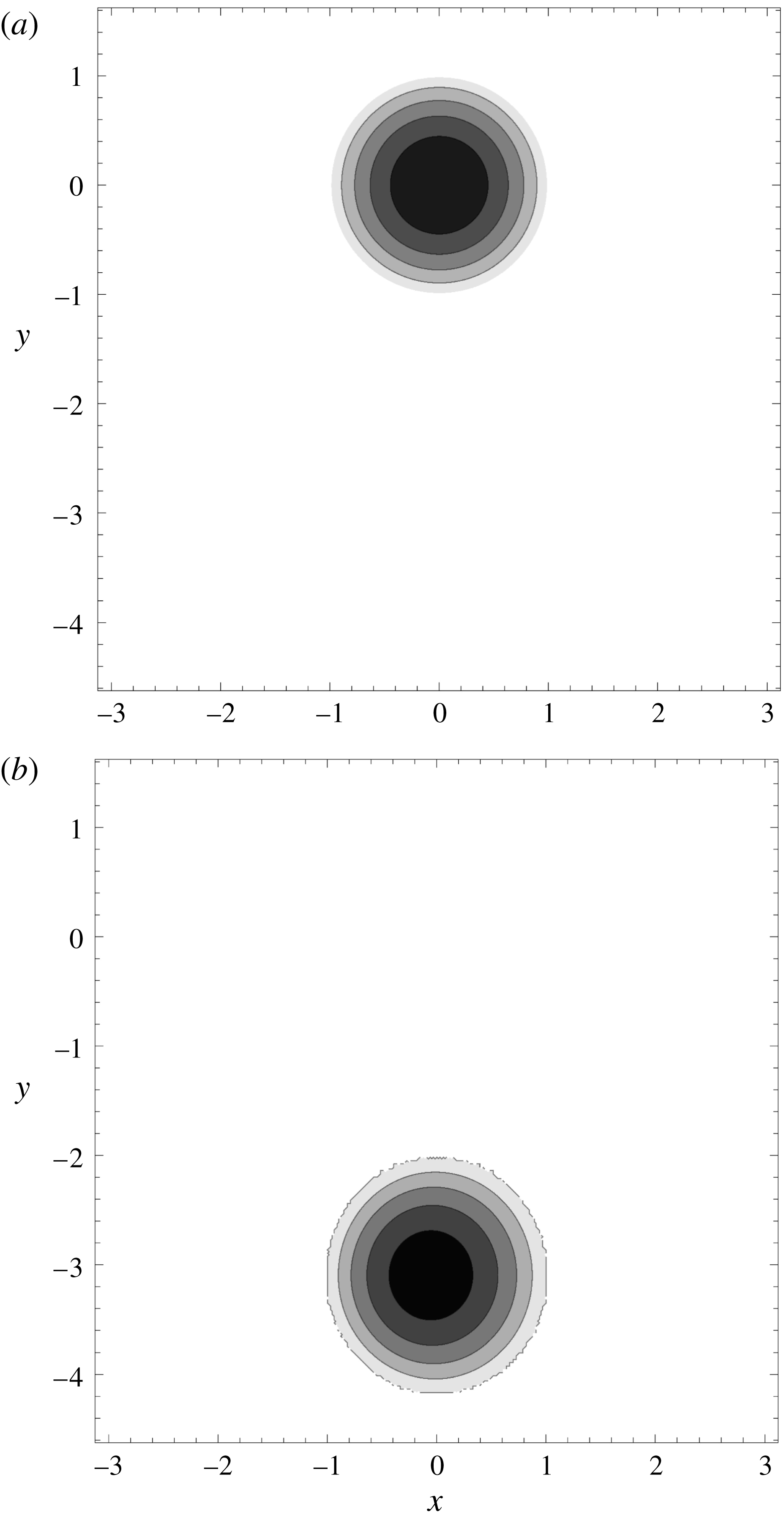
Figure 3(a) is a contour plot of the initial height
 $h(x,y,0)$
with
 $a=1$
and
 $\widetilde{h}_{0}=0.4$
(corresponding to maximum dimensional height of 224 m and a diameter of 200 km for the initial abyssal dome) for the contour intervals
 $0,0.08,0.16,\ldots ,0.4$
, respectively. The initial abyssal dome or pool is radially symmetric and is centred (for convenience) at
 $x=y=0$
. The volume of water within the abyssal dome (4.17) is given by
 $\unicode[STIX]{x03C0}\widetilde{h}_{0}\,a^{2}/2\simeq 0.63$
for these parameter values, which dimensionally corresponds to a volume of approximately
 $3520~\text{km}^{3}$
. The mass conservation equation (2.7) implies that volume is conserved as the abyssal dome propagates along the slope.
Figure 3(b) is a contour plot of the height
 $h(x,y,3)$
, i.e. when
 $t=3$
, corresponding dimensionally to approximately 90 days. As the abyssal dome propagates equatorward, the radial symmetry is lost (see figure 3
b). This is a consequence of (4.4), which has
 $|\text{d}y/\text{d}t|$
(the meridional speed of a point of constant phase within the abyssal dome, which is not to be confused with the Eulerian meridional fluid speed as determined by (2.5)) increasing equatorward for decreasing
 $y$
. As a result, the equatorward ‘face’ travels slightly faster equatorward than the poleward ‘face’ of the abyssal pool and the initially radially symmetric abyssal dome deforms into an elliptical-like shape where the major axis is oriented in the along-slope direction. In addition, from (4.3), we see that the upslope motion is proportional to the height of the abyssal dome
 $h>0$
. Consequently, the point of maximum height drifts upslope from its initial ‘centred’ position at
 $x=0$
as
 $t$
increases at a faster rate than the upslope motion associated with other points within the abyssal dome. This induces further asymmetry within the abyssal dome in addition to the elliptical-like shape (i.e. the height contours are not ‘pure’ ellipses). The location and value of the point of maximum height will be explicitly determined later in this section.


The evolution of the boundary of the abyssal dome into an elliptical-like shape as it propagates equatorward can be exactly determined. The boundary of the abyssal pool as a function of time is given by
 $$\begin{eqnarray}\unicode[STIX]{x1D707}^{2}(x,y,t)+\unicode[STIX]{x1D702}^{2}(y,t)=a^{2},\end{eqnarray}$$
which implies, as a result of (4.21), that
 $h(x,y,t)=0$
. However, since
 $h_{0}(\unicode[STIX]{x1D707},\unicode[STIX]{x1D702})=0$
on the abyssal dome boundary, it follows from (4.13) that
 $\unicode[STIX]{x1D707}=x$
exactly on the boundary (this implies that the groundings located at
 $x=\pm a$
do not shift up- or downslope as the dome propagates equatorward) so that substituting in (4.12) implies that the along-slope position of the abyssal dome boundary, denoted as
 $y_{b}(x,t)$
, is given by
 $$\begin{eqnarray}x^{2}+\left[-1+\sqrt{(1+\unicode[STIX]{x1D6FD}y_{b})^{2}+2\unicode[STIX]{x1D6FD}t}\right]^{2}\Big/\unicode[STIX]{x1D6FD}^{2}=a^{2},\end{eqnarray}$$
which can be rearranged into
 $$\begin{eqnarray}y_{b}(x,t)=\frac{-1+\sqrt{(1\pm \unicode[STIX]{x1D6FD}\sqrt{a^{2}-x^{2}})^{2}-2\unicode[STIX]{x1D6FD}t}}{\unicode[STIX]{x1D6FD}},\end{eqnarray}$$
with
 $-a\leqslant x\leqslant a$
.
Unlike the internal spatial structure of the abyssal dome, its boundary remains symmetrical about
 $x=0$
, i.e.
 $y_{b}(-x,t)=y_{b}(x,t)$
. The along-slope velocity of a point on the abyssal dome boundary can be written in the form
 $$\begin{eqnarray}\frac{\unicode[STIX]{x2202}y_{b}}{\unicode[STIX]{x2202}t}=-\frac{1}{1+\unicode[STIX]{x1D6FD}y_{b}},\end{eqnarray}$$
from which we conclude that the along-slope velocity of a point on the boundary is the Nof velocity (Nof Reference Nof1983) understood in the context of a mid-latitude
 $\unicode[STIX]{x1D6FD}$
-plane. Exploiting the ‘smallness’ of
 $\unicode[STIX]{x1D6FD}$
, it follows that
 $$\begin{eqnarray}y_{b}(x,t)\simeq -t-\unicode[STIX]{x1D6FD}t^{2}/2\pm (1+\unicode[STIX]{x1D6FD}t)\sqrt{a^{2}-x^{2}}+O(\unicode[STIX]{x1D6FD}^{2}).\end{eqnarray}$$
The first two terms of this asymptotic relation are the unsteady along-slope translation for the boundary that are independent of
 $x$
and, in the present context, the third term is responsible for an
 $O(2\unicode[STIX]{x1D6FD}t)$
increase, as
 $t$
increases, in the along-slope distance between the poleward and equatorward points on the boundary for fixed
 $x$
, i.e.
 $$\begin{eqnarray}y_{b}(x,t)|_{poleward}-y_{b}(x,t)|_{equatorward}=2(1+\unicode[STIX]{x1D6FD}t)\sqrt{a^{2}-x^{2}}.\end{eqnarray}$$
It is this
 $\unicode[STIX]{x1D6FD}$
-induced stretching in the distance (for the reasons given above) that results in the elliptical-like shape developing in the abyssal dome boundary as it propagates equatorward with the major axis forming in the along-slope direction. In the absence of
 $\unicode[STIX]{x1D6FD}$
, the along-slope distance between the poleward and equatorward points on the boundary for fixed
 $x$
would be just
 $2\sqrt{a^{2}-x^{2}}$
, which would correspond to the dome boundary being a circle of radius
 $a$
, as it is initially.
The maximum height
 $h_{max}(t)$
of the abyssal dome and its coordinate location
 $(x_{max}(t),y_{max}(t))$
are determined by
 $$\begin{eqnarray}\displaystyle & \unicode[STIX]{x1D735}h(x,y,t)=\mathbf{0}\quad \Longrightarrow \quad (x,y)=(x_{max}(t),y_{max}(t)), & \displaystyle\end{eqnarray}$$
 $$\begin{eqnarray}\displaystyle & h_{max}(t)\equiv h(x_{max},y_{max},t), & \displaystyle\end{eqnarray}$$
which, after a little algebra, can be shown to result in
 $$\begin{eqnarray}\displaystyle & x_{max}(t)=\unicode[STIX]{x1D6E4}(y_{max},t)(1-\unicode[STIX]{x1D702}^{2}(y_{max},t)/a^{2}), & \displaystyle\end{eqnarray}$$
 $$\begin{eqnarray}\displaystyle & \displaystyle y_{max}(t)=\frac{-1+\sqrt{\unicode[STIX]{x1D701}^{2}-2\unicode[STIX]{x1D6FD}t}}{\unicode[STIX]{x1D6FD}}, & \displaystyle\end{eqnarray}$$
where
 $\unicode[STIX]{x1D701}(t)$
is the continuous simple real root of the fourth-order polynomial
 $$\begin{eqnarray}\unicode[STIX]{x1D701}^{4}-\unicode[STIX]{x1D701}^{3}-\unicode[STIX]{x1D6FD}t\unicode[STIX]{x1D701}^{2}+\unicode[STIX]{x1D6FD}t(1-(\unicode[STIX]{x1D6FD}a)^{2})=0,\end{eqnarray}$$
where
 $\unicode[STIX]{x1D701}(0)=1~\Longrightarrow ~x_{max}(0)=y_{max}(0)=0$
.
Perhaps surprisingly, given the quasi-linearity of the underlying dynamics, the along-slope position of the point of maximum height
 $y_{max}(t)$
is independent of the abyssal dome height parameter
 $\widetilde{h}_{0}$
. However, the cross-slope position of the point of maximum height
 $x_{max}(t)$
depends linearly (as might be expected) on the abyssal dome height parameter
 $\widetilde{h}_{0}$
. Since it follows from (4.20) that
 $\unicode[STIX]{x1D6E4}(y_{max},t)\leqslant 0$
, we have
 $x_{max}(t)\leqslant 0$
from (4.31) (necessarily
 $|\unicode[STIX]{x1D702}|\leqslant a$
) so that the point of maximum height moves upslope from its initial location at
 $x_{max}(0)=0$
as the dome propagates equatorward.
Exploiting the ‘smallness’ of
 $\unicode[STIX]{x1D6FD}$
, an asymptotic analysis of (4.33) shows that
 $$\begin{eqnarray}\unicode[STIX]{x1D701}\simeq 1+a^{2}\unicode[STIX]{x1D6FD}^{3}t(1+2\unicode[STIX]{x1D6FD}t)+O(\unicode[STIX]{x1D6FD}^{6}),\end{eqnarray}$$
implying that
 $$\begin{eqnarray}\displaystyle & y_{max}\simeq -t(1+\unicode[STIX]{x1D6FD}t/2)+O(\unicode[STIX]{x1D6FD}^{2}), & \displaystyle\end{eqnarray}$$
 $$\begin{eqnarray}\displaystyle & x_{max}\simeq -\unicode[STIX]{x1D6FD}\widetilde{h}_{0}t(1+\unicode[STIX]{x1D6FD}t/2)+O(\unicode[STIX]{x1D6FD}^{3}) & \displaystyle\end{eqnarray}$$
and
 $$\begin{eqnarray}h_{max}\simeq \widetilde{h}_{0}[1-\unicode[STIX]{x1D6FD}t(1+\unicode[STIX]{x1D6FD}t/2)]+O(\unicode[STIX]{x1D6FD}^{3}).\end{eqnarray}$$
To the level of approximation in (4.35)–(4.37), the abyssal dome radius
 $a$
has no effect on the propagation characteristics of the point of maximum height. Detailed calculation based on (4.30)–(4.33) shows that the equatorward and upslope motion in
 $y_{max}$
and
 $x_{max}$
, respectively, is marginally slowed, and the reduction in
 $h_{max}$
is marginally retarded, as
 $a$
increases, but the effect is very weak. For example, doubling the abyssal dome radius to
 $a=2$
led to less than a
 $5.3\times 10^{-4}\,\%$
variation in
 $x_{max}$
,
 $y_{max}$
and
 $h_{max}$
as compared to the values for
 $a=1$
.
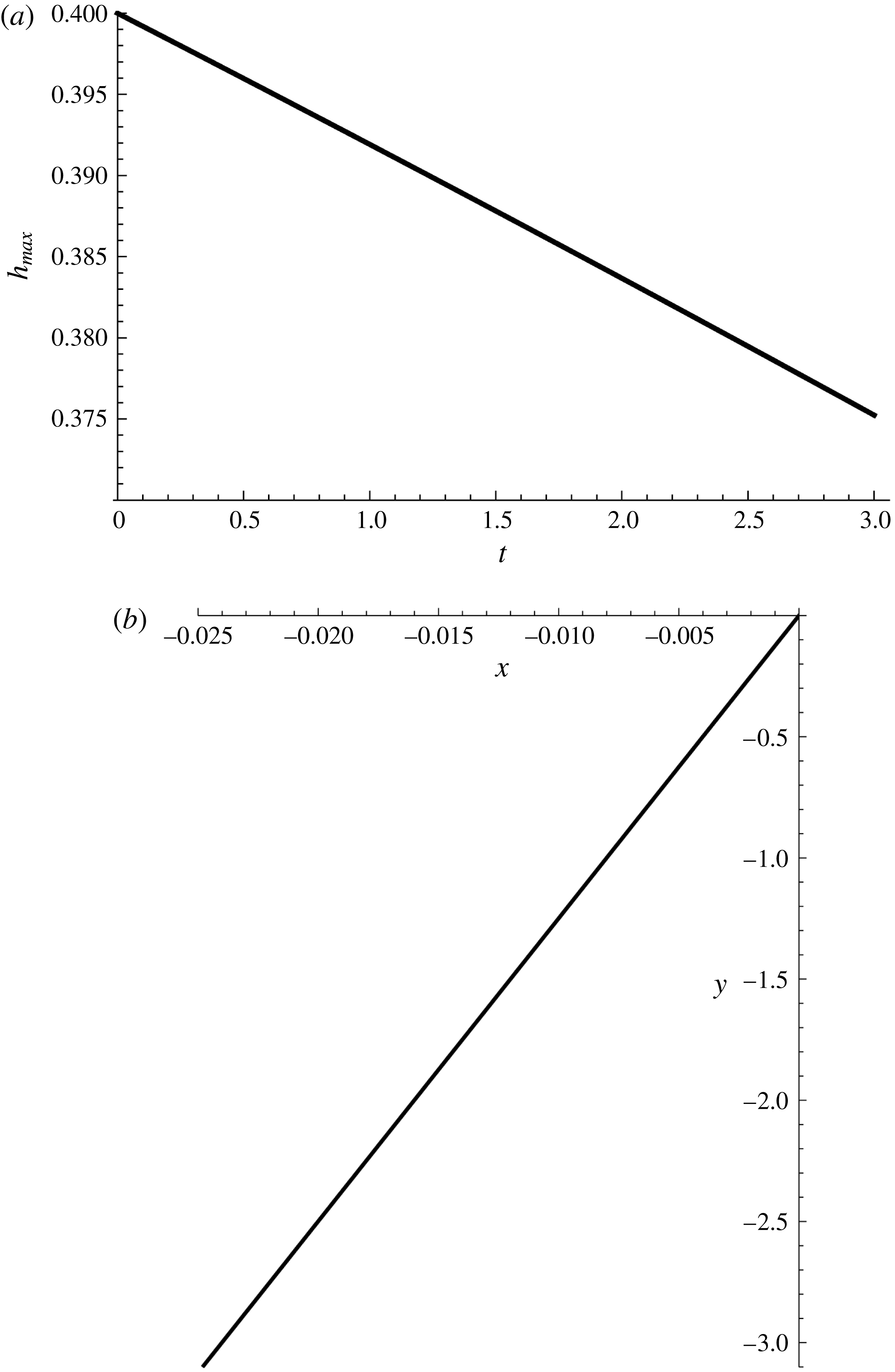
Figures 4(a) and 4(b), respectively, show the maximum height
 $h_{max}(t)$
and its coordinates
 $(x_{max}(t),y_{max}(t))$
versus
 $t$
for the interval
 $0\leqslant t\leqslant 3$
as determined from (4.30) to (4.33). Figure 4(a) shows the approximately linear decrease in
 $h_{max}(t)$
from its initial value of 0.4 to its value at
 $t=3$
of approximately 0.375. The decrease in
 $h_{max}(t)$
as the abyssal dome propagates equatorward is a consequence of the conservation of potential vorticity and the decreasing value of the Coriolis parameter as
 $y$
decreases. Figure 4(b) shows the equatorward and slightly upslope approximately linear trajectory of
 $(x_{max}(t),y_{max}(t))$
from its initial position of
 $(0,0)$
to the location at
 $t=3$
with coordinates approximately
 $(-0.025,-3.09)$
. It is noted that the asymptotic relations (4.35)–(4.37) very accurately reproduce the exact results for
 $(x_{max},y_{max})$
and
 $h_{max}$
at
 $t=3$
. The equatorward motion of
 $h_{max}(t)$
is primarily a consequence of the underlying geostrophic balance for the grounded abyssal dome on the sloping bottom, which holds even if
 $\unicode[STIX]{x1D6FD}=0$
(i.e. on a
 $f$
-plane). The upslope trajectory in
 $h_{max}(t)$
is, physically, purely a consequence of the Coriolis effect associated with
 $\unicode[STIX]{x1D6FD}$
, i.e. the Coriolis parameter decreasing as
 $y$
decreases.
(a) Graph of the maximum height
 $h_{max}(t)$
for the propagating abyssal dome for the time interval
 $0\leqslant t\leqslant 3$
. (b) Graph of the path
 $(x_{max}(t),y_{max}(t))$
for the propagating abyssal dome for the time interval
 $0\leqslant t\leqslant 3$
.

5 Time-dependent boundary-value solution
Let us consider the time-dependent boundary-value problem for which
 $$\begin{eqnarray}h(x,y_{0},t)=h_{0}(x,t),\end{eqnarray}$$
where
 $h_{0}(x,t)$
is a given across-slope abyssal height profile along
 $y=y_{0}$
. This type of time-dependent boundary-value problem is motivated by considering the impact that, for example, periodic seasonal variations in the upstream flow, or an isolated or one-time upstream increase or decrease in volume transport, might have on downstream abyssal current structure.
The characteristic equations associated with (2.9) for this time-dependent boundary value can be written in the form
 $$\begin{eqnarray}\displaystyle & \displaystyle \frac{\text{d}t}{\text{d}s}=1\quad \text{with }t|_{s=0}=\unicode[STIX]{x1D702}, & \displaystyle\end{eqnarray}$$
 $$\begin{eqnarray}\displaystyle & \displaystyle \frac{\text{d}x}{\text{d}s}=-\frac{\unicode[STIX]{x1D6FD}h}{(1+\unicode[STIX]{x1D6FD}y)^{2}}-\frac{\unicode[STIX]{x2202}_{y}h_{B}}{1+\unicode[STIX]{x1D6FD}y}\quad \text{with }x|_{s=0}=\unicode[STIX]{x1D707}, & \displaystyle\end{eqnarray}$$
 $$\begin{eqnarray}\displaystyle & \displaystyle \frac{\text{d}y}{\text{d}s}=\frac{\unicode[STIX]{x2202}_{x}h_{B}}{1+\unicode[STIX]{x1D6FD}y}\quad \text{with }y|_{s=0}=y_{0}, & \displaystyle\end{eqnarray}$$
 $$\begin{eqnarray}\displaystyle & \displaystyle \frac{\text{d}h}{\text{d}s}=\frac{\unicode[STIX]{x1D6FD}(\unicode[STIX]{x2202}_{x}h_{B})h}{(1+\unicode[STIX]{x1D6FD}y)^{2}}\quad \text{with }h|_{s=0}=h_{0}(\unicode[STIX]{x1D707},\unicode[STIX]{x1D702}), & \displaystyle\end{eqnarray}$$
where
 $s$
is the characteristic coordinate ‘along’ the characteristics and the time-dependent boundary height profile
 $h_{0}(\unicode[STIX]{x1D707},\unicode[STIX]{x1D702})$
is parametrized in terms of
 $\unicode[STIX]{x1D707}$
and
 $\unicode[STIX]{x1D702}$
, the characteristic coordinates associated with
 $x$
and
 $t$
, respectively.
As in the initial-value or Cauchy problem, three immediate integrations are possible. It follows from (5.2) that
 $$\begin{eqnarray}t=s+\unicode[STIX]{x1D702}.\end{eqnarray}$$
From (5.4) and (5.5) one obtains
 $$\begin{eqnarray}h=\frac{1+\unicode[STIX]{x1D6FD}y}{1+\unicode[STIX]{x1D6FD}y_{0}}h_{0}(\unicode[STIX]{x1D707},\unicode[STIX]{x1D702}).\end{eqnarray}$$
It follows from (5.3)–(5.5) that
 $$\begin{eqnarray}h+h_{B}(x,y)=h_{0}(\unicode[STIX]{x1D707},\unicode[STIX]{x1D702})+h_{B}(\unicode[STIX]{x1D707},y_{0}).\end{eqnarray}$$
Equations (5.7) and (5.8) can be combined to give
 $$\begin{eqnarray}h_{B}(x,y)=\frac{\unicode[STIX]{x1D6FD}(y_{0}-y)}{1+\unicode[STIX]{x1D6FD}y_{0}}\,h_{0}(\unicode[STIX]{x1D707},\unicode[STIX]{x1D702})+h_{B}(\unicode[STIX]{x1D707},y_{0}),\end{eqnarray}$$
which is the analogue of (4.10) for the time-dependent boundary-value problem. As in the initial-value problem, this is as far as one can go analytically for general topography. In general, one must numerically solve (5.3) and (5.4) to find an additional relationship connecting
 $(x,t)$
and
 $(\unicode[STIX]{x1D707},\unicode[STIX]{x1D702})$
, which will then complete the solution. However, for a linearly sloping bottom, substantial further analytical progress is possible. In the limit where there is no time dependence in the boundary condition
 $h_{0}$
, i.e.
 $h_{0}=h_{0}(x)$
, equations (5.7) and (5.9) reduce exactly to the nonlinear steady solution (3.2) and (3.3).
5.1 Linearly sloping bottom
In the approximation that
 $h_{B}=-x,$
the nonlinear solution to the time-dependent boundary-value problem, although implicit, can be completely determined. Assuming
 $h_{B}=-x$
, it follows from (5.4) and (5.6) that
 $$\begin{eqnarray}\unicode[STIX]{x1D702}(y,t)=t+\frac{(1+\unicode[STIX]{x1D6FD}y)^{2}-(1+\unicode[STIX]{x1D6FD}y_{0})^{2}}{2\unicode[STIX]{x1D6FD}},\end{eqnarray}$$
which when substituted into (5.9) yields
 $$\begin{eqnarray}x=\unicode[STIX]{x1D707}+\frac{\unicode[STIX]{x1D6FD}(y-y_{0})}{1+\unicode[STIX]{x1D6FD}y_{0}}\,h_{0}\left(\unicode[STIX]{x1D707},t+\frac{(1+\unicode[STIX]{x1D6FD}y)^{2}-(1+\unicode[STIX]{x1D6FD}y_{0})^{2}}{2\unicode[STIX]{x1D6FD}}\right).\end{eqnarray}$$
We note that the initial conditions associated with the characteristic equations imply
 $\unicode[STIX]{x1D702}(y_{0},t)=t$
and
 $\unicode[STIX]{x1D707}(x,y_{0},t)=x$
. Thus, given
 $(x,y,t)$
,
 $\unicode[STIX]{x1D702}$
is determined by (5.10) and
 $\unicode[STIX]{x1D707}$
implicitly by (5.11), and consequently
 $h(x,y,t)$
by (5.7). While there are any number of time-dependent boundary conditions one can consider, here we examine two idealized but illustrative examples where a complete analytical description is possible.
5.2 Time-dependent boundary condition with upslope and downslope groundings
As a time-dependent boundary-value example for which it is possible to write down an explicit nonlinear solution, let us consider the linearly sloping bottom
 $h_{B}=-x$
with the abyssal height boundary profile along
 $y=y_{0}$
given by
 $$\begin{eqnarray}h_{0}(x,t)=\left\{\begin{array}{@{}ll@{}}\widetilde{h}_{0}(t)\{1-[x-b(t)]^{2}/a^{2}(t)\}\quad & \text{if }|x-b(t)|\leqslant a(t),\\ 0\quad & \text{if }|x-b(t)|>a(t),\end{array}\right.\end{eqnarray}$$
with
 $0<\widetilde{h}_{0}(t)<a(t)/2$
(ensuring that the meridional velocity is strictly equatorward along
 $y=y_{0}$
, which in turn ensures that a shock does not develop in the solution in the region and over the time of interest). The abyssal height (5.12) corresponds to a ‘parabolic’ cross-slope boundary profile with time-dependent half-width
 $a(t)>0$
and maximum height
 $\widetilde{h}_{0}(t)>0$
located at
 $x=b(t)$
, which possesses time-dependent upslope and downslope groundings located at
 $x=b(t)\pm a(t)$
. In the present circumstance,
 $a(t)$
,
 $b(t)$
and
 $\widetilde{h}_{0}(t)$
are assumed given.
Substitution of (5.12) into (5.11) implies, after a little algebra, that
 $$\begin{eqnarray}\unicode[STIX]{x1D707}(x,y,t)=\left\{\begin{array}{@{}ll@{}}\unicode[STIX]{x1D6F9}(x,y,t)\quad & \text{if }|\unicode[STIX]{x1D6F9}|\leqslant a(\unicode[STIX]{x1D702}),\\ x\quad & \text{if }|\unicode[STIX]{x1D6F9}|>a(\unicode[STIX]{x1D702}),\end{array}\right.\end{eqnarray}$$
where
 $$\begin{eqnarray}\unicode[STIX]{x1D6F9}(x,y,t)\equiv b(\unicode[STIX]{x1D702})+\frac{2a(\unicode[STIX]{x1D702})[\unicode[STIX]{x1D6E4}+x\,-b(\unicode[STIX]{x1D702})]}{a(\unicode[STIX]{x1D702})+\sqrt{4\unicode[STIX]{x1D6E4}^{2}+4[x-b(\unicode[STIX]{x1D702})]\unicode[STIX]{x1D6E4}+a^{2}(\unicode[STIX]{x1D702})}},\end{eqnarray}$$
with
 $$\begin{eqnarray}\unicode[STIX]{x1D6E4}(y,t)\equiv \frac{\unicode[STIX]{x1D6FD}(y_{0}-y)\widetilde{h}_{0}(\unicode[STIX]{x1D702})}{1+\unicode[STIX]{x1D6FD}y_{0}},\end{eqnarray}$$
where
 $\unicode[STIX]{x1D702}(y,t)$
is given by (5.10). Again, we note that
 $\unicode[STIX]{x1D6F9}(x,y_{0},t)=x$
,
 $\unicode[STIX]{x1D6E4}(y_{0},t)=0$
and that
 $\unicode[STIX]{x1D6E4}(y,t)>0$
for
 $y<y_{0}$
. Substitution of (5.10) and (5.12)–(5.15) into (5.7) determines
 $h(x,y,t)$
.
5.3 Time-limited surge in the equatorward transport along the poleward boundary
Here, we describe the model prediction associated with the effect that a time-limited upstream pulse or surge in the equatorward transport along the poleward boundary has on the grounded abyssal current in the mid-latitude domain. Physically, this scenario could correspond to a situation where, for example, seasonal variations have led to increased time-limited deep-water formation in high latitudes poleward of our domain. (We could equally well have examined the opposite effect, that is, a reduction in equatorward transport along
 $y=y_{0}$
. How the results would qualitatively differ from those described here will be self-evident.) Again, we note that the solution described here is one of the few known exact nonlinear solutions for a time-dependent oceanographic flow that crosses the planetary vorticity gradient.
To make our description concrete, we set
 $$\begin{eqnarray}a(t)=1+0.3\,\text{sech}(t-4),\quad \widetilde{h}_{0}(t)=0.45+0.195\,\text{sech}(t-4)\quad \text{and}\quad b(t)=0.\end{eqnarray}$$
In the absence of any time variation, the upslope and downslope groundings associated with the boundary condition
 $h_{0}(x,t)$
are located at
 $\pm 1$
, which implies an abyssal current width along
 $y=y_{0}$
of 2 (or dimensionally 200 km), and where the maximum non-dimensional height above the topography is 0.45 (or dimensionally approximately 250 m) and is located at
 $x=0$
. At the time of maximum transport surge along
 $y=y_{0}$
, which occurs at
 $t=4$
(or dimensionally approximately 120 days after
 $t=0$
when the surge ‘just starts’ to occur), the abyssal current width is increased by 30 % to 260 km, and the maximum height above the topography is increased by approximately 43 % to approximately 360 m. These idealized parameter values ensure that
 $v(x,y_{0},t)<0$
for all
 $(x,t)$
, which ensures that no shock will form in the solution in the region of interest. In addition, choosing
 $b(t)=0$
implies that there is no cross-slope movement in the point of maximum height along
 $y=y_{0}$
. We will examine a situation, corresponding to the formation of a downslope loop or plume along the downslope grounding, where
 $b$
varies in time, later in this section.
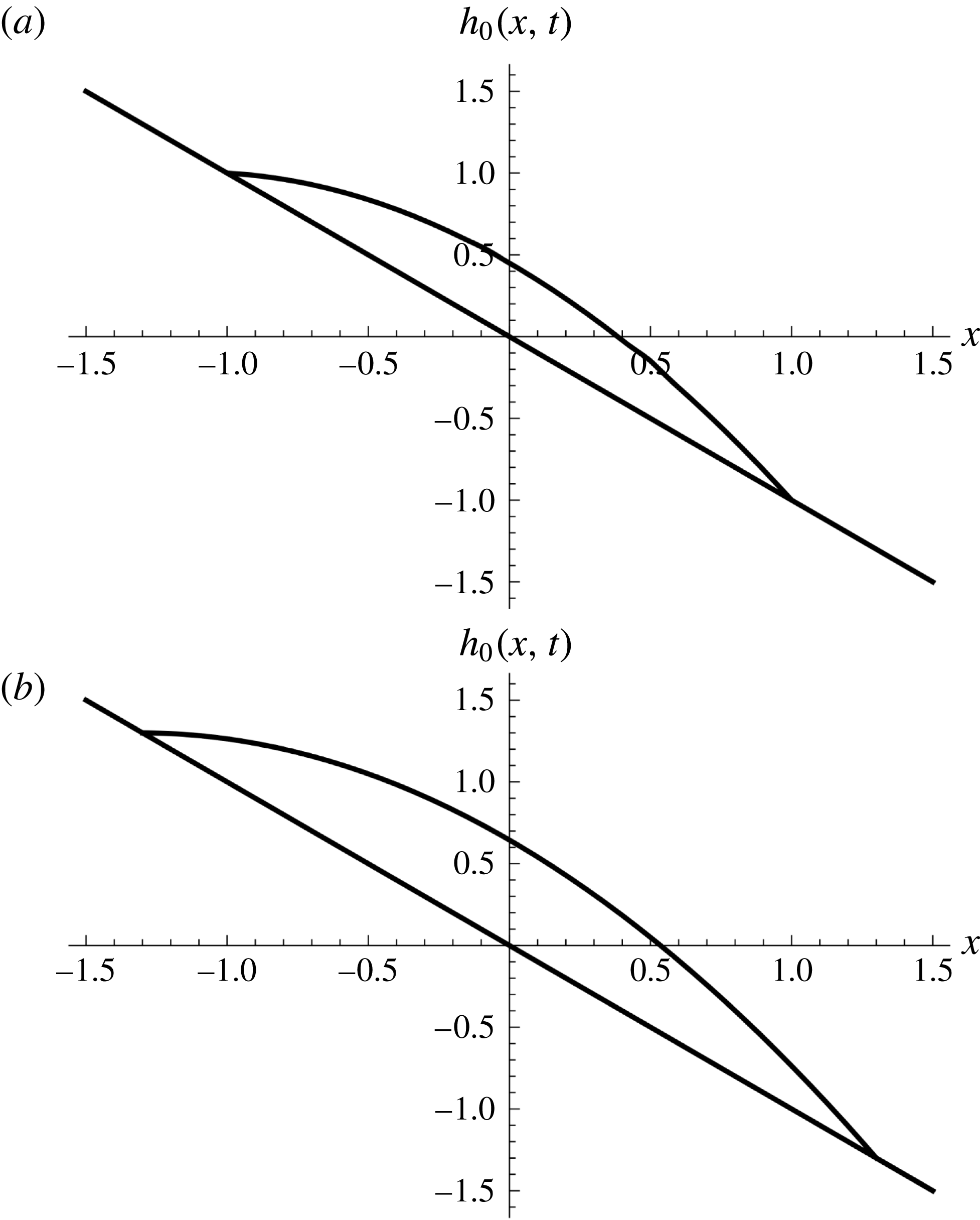
Figure 5(a,b) are graphs of the abyssal current height on top of the sloping topography versus
 $x$
along
 $y=y_{0}$
, i.e.
 $h_{0}$
, in the absence any time variation in
 $a$
and
 $\widetilde{h}_{0}$
, and at
 $t=4$
(corresponding to the time of maximum transport surge), respectively. In figure 5(b) the downslope and upslope groundings in the abyssal current height are displaced symmetrically in the downslope and upslope directions by 0.3, respectively, and the maximum height is increased by 0.195, as compared to that in figure 5(a).
(a) Graph of the abyssal current height
 $h_{0}$
on the sloping bottom along
 $y=y_{0}$
prior to the onset of the surge in volume transport. (b) Graph of the abyssal current height
 $h_{0}$
on the sloping bottom along
 $y=y_{0}$
at the time of maximum transport surge
 $(t=4)$
.

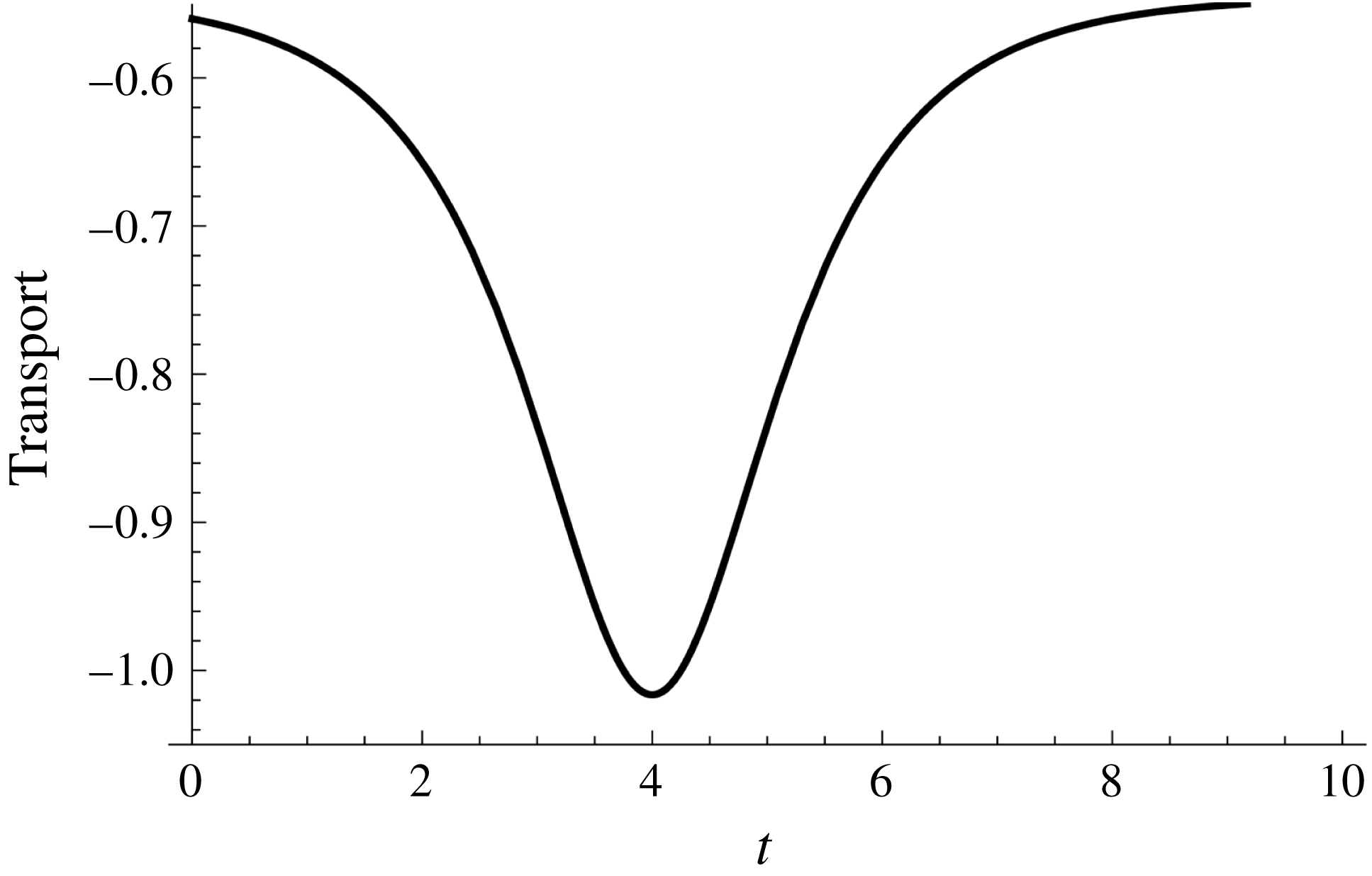
The non-dimensional meridional transport along
 $y=y_{0}$
, denoted by
 $T_{0}(t)$
, will be given by
 $$\begin{eqnarray}T_{0}(t)=\int _{b(t)-a(t)}^{b(t)+a(t)}v(x,y_{0},t)h_{0}(x,t)\,\text{d}x=-\frac{4a(t)\widetilde{h}_{0}(t)}{3(1+\unicode[STIX]{x1D6FD}y_{0})}.\end{eqnarray}$$
In the absence of any time variation,
 $T_{0}\simeq -0.55$
(or dimensionally approximately
 $-1.22~\text{Sv}$
;
 $1~\text{Sv}=10^{6}~\text{m}^{3}~\text{s}^{-1}$
). At the time of maximum transport surge along
 $y=y_{0}$
,
 $T_{0}(4)\simeq -1.02$
(or dimensionally approximately
 $-2.28~\text{Sv}$
), corresponding to an 87 % increase in equatorward transport along
 $y=y_{0}$
. For
 $t>4$
, the surge in the equatorward transport diminishes along
 $y=y_{0}$
. It is important to emphasize that this is an idealized scenario meant to elucidate the dynamics rather than to model a specific oceanographic event (although that would be interesting as well). These transport values are reasonably consistent with observations of the ‘deep’ transport associated with ‘overflow/lower deep water’ associated with the DWBC near Cape Cod (e.g. Joyce et al.
Reference Joyce, Dunworth-Baker, Pickart and Waterman2005). Figure 6, which is a graph of
 $T_{0}(t)$
versus
 $t$
for
 $0\leqslant t\leqslant 10$
, shows the increase in the equatorward transport along
 $y=y_{0}$
from its value at
 $t=0$
, when the surge is just starting to occur, to its maximum when
 $t=4$
, and its subsequent decline back to its value before the surge occurs, which for all practical calculations is the case when
 $t=10$
.
Graph of the meridional volume transport
 $T_{0}(t)$
along the poleward boundary
 $y=y_{0}$
versus
 $t$
for
 $0\leqslant t\leqslant 10$
.

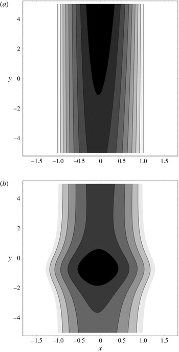
Figures 7(a) and 7(b) are, respectively, contour plots of
 $h(x,y,t)$
for
 $t=0$
and
 $t=10$
, corresponding, respectively, to a time that is just immediately before the surge in transport occurs along
 $y=y_{0}$
and a time for which the anomaly associated with the transport surge has propagated well into the interior of the mid-latitude domain. Figure 7(a) is qualitatively similar to the steady nonlinear solution described in Swaters (Reference Swaters2015a
). Figure 7(b) illustrates the spatially limited and equatorward-propagating varicose-like anomaly within the grounded abyssal current that is generated by the time-limited transport surge along the poleward boundary
 $y=y_{0}$
. As the anomaly propagates equatorward, the point of maximum height decreases and shifts upslope as a consequence of the planetary vorticity gradient. To leading order, the along-slope position of the point of maximum height is determined by, essentially, the geostrophic (Nof Reference Nof1983) balance (understood in the context of a mid-latitude
 $\unicode[STIX]{x1D6FD}$
-plane).
(a) Contour plot of the height
 $h$
prior to the onset of the surge in transport along the poleward boundary. The contour interval is approximately 0.05. (b) Contour plot of the height
 $h(x,y,10)$
when the transport surge has fully propagated into the domain. The contour interval is approximately 0.12.

The point of maximum height
 $h_{max}(t)$
of the anomaly associated with the transport surge as illustrated in figure 7(b) and its coordinate location
 $(x_{max}(t),y_{max}(t))$
are determined by
 $$\begin{eqnarray}\unicode[STIX]{x1D735}h(x,y,t)=\mathbf{0}\quad \Longrightarrow \quad (x,y)=(x_{max}(t),y_{max}(t)),\end{eqnarray}$$
which, after a little algebra, can be shown to result in
 $$\begin{eqnarray}x_{max}(t)=-\frac{\unicode[STIX]{x1D6FD}(y_{0}-y_{max})\widetilde{h}_{0}[\unicode[STIX]{x1D702}(y_{max},t)]}{1+\unicode[STIX]{x1D6FD}y_{0}}<0,\end{eqnarray}$$
where
 $y_{max}(t)$
is a continuous simple real root of
 $$\begin{eqnarray}\displaystyle & & \displaystyle 0.195(1+\unicode[STIX]{x1D6FD}y_{max})^{2}\,\text{sech}[\unicode[STIX]{x1D702}(y_{max},t)-4]\tanh [\unicode[STIX]{x1D702}(y_{max},t)-4]\nonumber\\ \displaystyle & & \displaystyle \quad =\unicode[STIX]{x1D6FD}(0.45+0.195\,\text{sech}[\unicode[STIX]{x1D702}(y_{max},t)-4]),\end{eqnarray}$$
and, consequently, where
 $$\begin{eqnarray}h_{max}(t)\equiv \frac{1+\unicode[STIX]{x1D6FD}y_{max}(t)}{1+\unicode[STIX]{x1D6FD}y_{0}}\,\widetilde{h}_{0}(\unicode[STIX]{x1D702}(y_{max},t)).\end{eqnarray}$$
Exploiting the ‘smallness’ of
 $\unicode[STIX]{x1D6FD}$
, an asymptotic analysis of (5.20) shows that
 $$\begin{eqnarray}\displaystyle & \displaystyle y_{max}\simeq y_{0}+4-t+\unicode[STIX]{x1D6FD}\{3.31+{\textstyle \frac{1}{2}}[(y_{0}+4-t)^{2}-y_{0}^{2}]\}+O(\unicode[STIX]{x1D6FD}^{2}), & \displaystyle\end{eqnarray}$$
 $$\begin{eqnarray}\displaystyle & \displaystyle x_{max}\simeq 0.645\unicode[STIX]{x1D6FD}(4-t)+O(\unicode[STIX]{x1D6FD}^{2}) & \displaystyle\end{eqnarray}$$
and
 $$\begin{eqnarray}h_{max}\simeq 0.645[1+\unicode[STIX]{x1D6FD}(4-t)]+O(\unicode[STIX]{x1D6FD}^{2}).\end{eqnarray}$$
The leading-order linear decrease in
 $y_{max}$
in (5.22) is independent of
 $\unicode[STIX]{x1D6FD}$
and is a consequence of the
 $f$
-plane geostrophic balance between the downslope gravity-driven acceleration of a grounded dense water mass (as compared to the ambient) sitting directly on a sloping bottom and the Coriolis effect (i.e. the Nof (Reference Nof1983) balance). The upslope drift in
 $x_{max}$
in (5.23) is purely a consequence of differential rotation. The
 $O(\unicode[STIX]{x1D6FD})$
linear decrease in
 $h_{max}$
in (5.24) is a consequence of the conservation of potential vorticity on the mid-latitude
 $\unicode[STIX]{x1D6FD}$
-plane. Note that to leading order
 $y_{max}\simeq y_{0}$
,
 $x_{max}\simeq 0$
and
 $h_{max}\simeq 0.645\equiv 0.45+0.195$
when
 $t=4$
, corresponding to the time when the transport surge is maximum along
 $y=y_{0}$
.
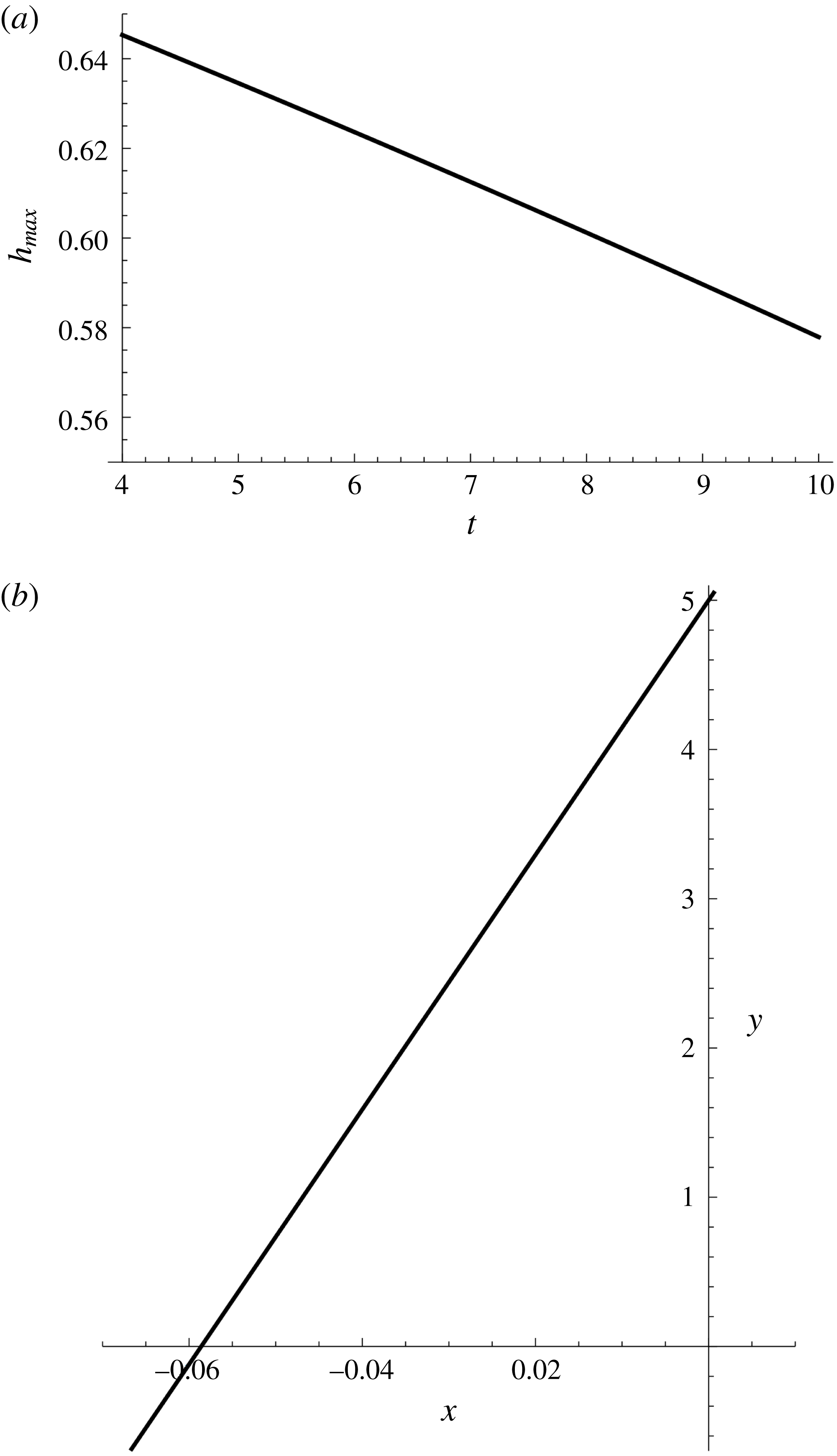
Figures 8(a) and 8(b), respectively, show the maximum height
 $h_{max}(t)$
and its coordinates
 $(x_{max}(t),y_{max}(t))$
versus
 $t$
for the interval
 $4\leqslant t\leqslant 10$
as determined from (5.19)–(5.21). Figure 8(a) shows the approximately linear decrease in
 $h_{max}(t)$
from its initial value of 0.645 at
 $t=4$
to its value at
 $t=10$
of approximately 0.58. Figure 8(b) shows the equatorward and slightly upslope approximately linear trajectory of
 $(x_{max}(t),y_{max}(t))$
from its leading-order position at
 $(0,y_{0})$
at
 $t=4$
to the location at
 $t=10$
with coordinates approximately
 $(-0.07,-0.67)$
.


5.4 Formation of a downslope plume or loop in the abyssal current along the poleward boundary
Here, we describe the resulting flow associated with a time-limited downslope shift in the cross-slope position of the boundary abyssal current’s centre of mass, or, equivalently in our model, the cross-slope position of the point of maximum height along
 $y=y_{0}$
. The resulting flow in the interior of the domain resembles a sinuous-like downslope loop or plume anomaly that propagates equatorward. It is remarked that the unstable modes associated with the baroclinic instability of grounded abyssal currents (see figure 9 in Swaters (Reference Swaters1991) and plate 1 in Swaters (Reference Swaters1998)) are along-slope propagating meanders that preferentially amplify along the downslope grounding growing into downslope plumes. It is suggested that the dynamics described here may be of relevance to the nonlinear along-slope propagation of these finite-amplitude plumes once they have formed. Again, we note that the solution described here is one of the few known exact nonlinear solutions for a time-dependent oceanographic flow that crosses the planetary vorticity gradient.
To make our description concrete, we set
 $$\begin{eqnarray}a(t)=1,\quad \widetilde{h}_{0}(t)=0.45\quad \text{and}\quad b(t)=\text{sech}(t-4).\end{eqnarray}$$
These choices correspond to holding fixed in time the width of the abyssal current along
 $y=y_{0}$
to be 2 (or dimensionally approximately 200 km) and its maximum height to be 0.45 (or dimensionally approximately 250 m) but allowing the cross-slope position of the maximum height to shift 1 non-dimensional unit (or approximately 100 km) downslope (when
 $t=4$
).
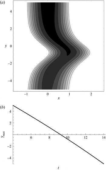
Figure 9(a) is a contour plot of the abyssal current height
 $h(x,y,t)$
for
 $t=10$
when the downslope plume or loop has propagated into the interior of the mid-latitude domain (
 $-5\leqslant y\leqslant 5$
). Prior to the formation of the downslope plume or loop
 $(t\ll 4)$
, a contour plot of
 $h(x,y,t)$
for our domain would look exactly like that shown in figure 7(a) (note, however, that figure 9(a) contains a larger range of
 $x$
-values as compared to figure 7(a)). The resulting anomaly in the abyssal current resembles a sinuous-like downslope finite-amplitude plume or loop. Owing to the conservation of potential vorticity, and as predicted by (5.7), the abyssal current height decreases as
 $y$
decreases.
(a) Contour plot of the height
 $h(x,y,10)$
when the downslope plume or loop has fully propagated into the domain. The contour interval is approximately 0.05. (b) Graph of the along-slope position
 $y_{max}(t)$
of the point of maximum downslope extent, or crest, associated with the downslope plume as seen in figure 9(a) versus
 $t$
for
 $0\leqslant t\leqslant 14$
.

The plume or loop propagates equatorward with equatorward speed increasing as
 $y$
decreases. It follows from (5.7), (5.10), (5.12) and (5.25) that the along-slope position of the crest, denoted by
 $y_{max}(t)$
, of the downslope plume or loop, i.e. its furthermost downslope extent, is given by
 $$\begin{eqnarray}\unicode[STIX]{x1D702}(y_{max},t)=4,\end{eqnarray}$$
which can be rearranged into
 $$\begin{eqnarray}y_{max}(t)=\frac{\sqrt{(1+\unicode[STIX]{x1D6FD}y_{0})^{2}+2\unicode[STIX]{x1D6FD}(4-t)}-1}{\unicode[STIX]{x1D6FD}},\end{eqnarray}$$
from which it follows that
 $$\begin{eqnarray}\frac{\text{d}y_{max}}{\text{d}t}=-\frac{1}{1+\unicode[STIX]{x1D6FD}y_{max}}.\end{eqnarray}$$
Equation (5.28) is, again, the statement that the equatorward speed of propagation of the downslope loop or plume is the Nof velocity (Nof Reference Nof1983) understood in the context of the mid-latitude
 $\unicode[STIX]{x1D6FD}$
-plane we are working with. Clearly, as
 $y_{max}$
decreases,
 $|\text{d}y_{max}/\text{d}t|$
increases (albeit gradually since
 $\unicode[STIX]{x1D6FD}\simeq 0.02$
for our scalings). Figure 9(b) is a graph of
 $y_{max}(t)$
versus
 $t$
for
 $4\leqslant t\leqslant 14$
. Figure 9(a) depicts a more or less linear equatorward translation of
 $y_{max}(t)$
as
 $t$
increases (the apparent linearity is a consequence of
 $\unicode[STIX]{x1D6FD}\simeq 0.02$
).
6 Conclusions
Observations, theoretical considerations and numerical simulations suggest that, in mid-latitudes away from the equator and from the polar source regions, hemispheric-scale abyssal flows, such as the Deep Western Boundary Current and Antarctic Bottom Water, are often grounded on the continental slope, in geostrophic balance, flow substantial distances coherently across the planetary vorticity gradient, are density- or gravity-driven, and are more or less topographically steered. The principal purpose of this paper was to examine these dynamics in a simple but nevertheless illuminating nonlinear time-dependent planetary geostrophic reduced-gravity model that describes density- or gravity-driven grounded abyssal meridional flow over sloping topography permitting groundings in the abyssal water height in a mid-latitude
 $\unicode[STIX]{x1D6FD}$
-plane. This model is an extension of the so-called planetary geostrophic wave equation, generalized to allow for meridional flow on a mid-latitude
 $\unicode[STIX]{x1D6FD}$
-plane with variable bottom topography.
Both steady and time-dependent exact solutions were examined. Nonlinear steady solutions can be obtained using the method of characteristics for arbitrary topography. It was shown that if the meridional velocity along the poleward boundary of the mid-latitude region of interest is equatorward, then no ‘shock’ can form in the solution within the mid-latitude
 $\unicode[STIX]{x1D6FD}$
-plane region. Qualitatively, the steady solutions are non-parallel equatorward-flowing currents (with an upslope velocity component), which speed up and diminish in height as a consequence of the conservation of meridional volume transport and potential vorticity. These qualitative features are consistent with observations and numerical simulations. The theory was illustrated for a simple example corresponding to an abyssal current that had a single upslope grounding. It is worthy of note that both the steady and time-dependent exact solutions described here are among the very few known exact solutions for meridional oceanographic flow across the planetary vorticity gradient.
The time-dependent equations could be solved using the method of characteristics. In general, the characteristic equations must be solved numerically, but in the case of linearly sloping bottom topography, they can be solved analytically, which allows for the qualitative properties to be easily described. Two types of time-dependent problems were examined. Exact nonlinear solutions could be found for the pure initial-value or Cauchy problem. In addition, exact solutions could be found for the nonlinear time-dependent boundary-value problem where a prescribed time-varying current is given along the poleward boundary of the mid-latitude
 $\unicode[STIX]{x1D6FD}$
-plane.
The initial-value theory was illustrated with two oceanographically relevant examples. The first initial condition corresponded to a parallel flow with no cross-slope shear in the along-slope velocity but which possesses a single grounding along its upslope flank. The current was seen to evolve towards an unsteady non-parallel equatorward shear flow with a ‘small’ upslope velocity component.
The second initial-value example considered was an initial isolated radially symmetric abyssal pool or dome. Mesoscale abyssal domes or pools that survive for months have been observed along the North American slope in the Atlantic Ocean. The abyssal dome is seen to travel equatorward ‘coherently’ with unsteady meridional and upslope velocity components. The initial radially symmetric abyssal height profile becomes elliptical in shape with the major axis oriented in the along-slope direction and the point of maximum height shifts upslope in relation to the major axis. There is a
 $\unicode[STIX]{x1D6FD}$
-induced decrease in the maximum height of the abyssal dome as it propagates equatorward as a consequence of the conservation of potential vorticity.
Two specific nonlinear time-dependent problems were examined. The first corresponds to a situation where a time-limited surge in the equatorward volume transport occurs in the grounded abyssal current along the poleward boundary of the mid-latitude
 $\unicode[STIX]{x1D6FD}$
-plane. This problem could be solved exactly and the time-dependent response of the abyssal current within the mid-latitude
 $\unicode[STIX]{x1D6FD}$
-plane domain was described. The second time-dependent boundary condition examined corresponds to the formation of a downslope plume or loop in the abyssal current along the poleward boundary of the mid-latitude domain. Downslope plumes or loops are formed during the baroclinic destabilization of these grounded abyssal currents on a sloping bottom. The nonlinear evolution and the equatorward propagation of the downslope plume or loop could be determined explicitly and was described.
It is very important to make explicit note of the fact that the model examined here has intentionally ignored many physical processes that are important, such as baroclinic, barotropic and Kelvin–Helmholtz instability, vertical entrainment and mixing between the overlying water column and the abyssal water mass, and bottom friction. Nevertheless, it is suggested that it is of interest to understand the fundamental geophysical fluid mechanics associated with the idealized low-frequency nonlinear dynamics that the observations and numerical simulations seem to suggest dominates the mid-latitude meridional transport of abyssal water masses along a continental slope. It is hoped that the results described here will help to provide some dynamical ‘guide posts’ for some of the processes observed in more complete analytical or numerical models for the hemispheric-scale meridional flow of grounded abyssal ocean waters.
Acknowledgements
The author is indebted to Professor A. Willmott, Newcastle University, UK for suggesting the examination of the nonlinear time-dependent boundary-value problem described in § 5. Preparation of this manuscript was supported in part by Discovery Research grants awarded by the Natural Sciences and Engineering Research Council (NSERC) of Canada.