2.3.1 Governing equations within the fluids

The flow in each fluid region is described by the non-dimensional continuity and Navier–Stokes equations, given below for fluids $j=1,2$ ,

(2.19a ) $$\begin{eqnarray}\displaystyle & \displaystyle u_{jx}+v_{jy}=0, & \displaystyle\end{eqnarray}$$

(2.19b ) $$\begin{eqnarray}\displaystyle & \displaystyle u_{jt}+u_{j}u_{jx}+v_{j}u_{jy}=-\frac{1}{r_{j}}p_{jx}+\frac{1}{Re_{j}}(u_{jxx}+u_{jyy}), & \displaystyle\end{eqnarray}$$

(2.19c ) $$\begin{eqnarray}\displaystyle & \displaystyle v_{jt}+u_{j}v_{jx}+v_{j}v_{jy}=-\frac{1}{r_{j}}p_{jy}+\frac{1}{Re_{j}}(v_{jxx}+v_{jyy})-\frac{1}{Fr^{2}}. & \displaystyle\end{eqnarray}$$

(2.20) $$\begin{eqnarray}\displaystyle & \displaystyle C_{t}+u_{1}C_{x}+v_{1}C_{y}=\frac{1}{Pe_{b}}(C_{xx}+C_{yy})-J_{m}, & \displaystyle\end{eqnarray}$$

(2.21) $$\begin{eqnarray}\displaystyle & \displaystyle M_{t}+u_{1}M_{x}+v_{1}M_{y}=\frac{1}{Pe_{m}}(M_{xx}+M_{yy})+J_{m}, & \displaystyle\end{eqnarray}$$

with the dimensionless flux $J_{m}$ given by

(2.22) $$\begin{eqnarray}J_{m}=K_{m}(C^{N}-M).\end{eqnarray}$$

The boundary conditions imposed on the channel walls are

(2.23a ) $$\begin{eqnarray}\displaystyle & \displaystyle \text{No slip: }u_{1}=0\quad \text{at }y=0,\quad \text{and}\quad u_{2}=1\quad \text{at }y=1, & \displaystyle\end{eqnarray}$$

(2.23b ) $$\begin{eqnarray}\displaystyle & \displaystyle \text{No penetration: }v_{1}=0\quad \text{at }y=0,\quad \text{and}\quad v_{2}=0\quad \text{at }y=1, & \displaystyle\end{eqnarray}$$

(2.23c ) $$\begin{eqnarray}\displaystyle & \displaystyle \text{No flux: }C_{y}=0\quad \text{at }y=0,\quad \text{and}\quad M_{y}=0\quad \text{at }y=0. & \displaystyle\end{eqnarray}$$

Table 1.

Non-dimensional parameters arising in the model formulation. Key to parameter names in table – $n$ : thickness ratio; $r$ : density ratio; $m$ : viscosity ratio; $Re$ : Reynolds number (note that $Re=Re_{1}=(m/r)Re_{2}$ );  $We$ : Weber number; $Ca$ : capillary number; $Fr$ : Froude number; $Bo$ : Bond number; $Ma$ : Marangoni number; $Pe_{s}$ , $Pe_{b}$ , $Pe_{m}$ : Peclét numbers (surface, bulk, micelle); $Bi$ : Biot number. The following parameters are also defined: $r_{j}=\unicode[STIX]{x1D70C}_{j}/\unicode[STIX]{x1D70C}_{1}$ and $m_{j}=\unicode[STIX]{x1D707}_{j}/\unicode[STIX]{x1D707}_{1}$ , $j=1,2$ , such that $r_{1}=1$ , $r_{2}=r$ and $m_{1}=1$ , $m_{2}=m$ .

2.3.2 Coupling conditions at the interface

Continuity of horizontal and vertical velocities at the interface gives

(2.24) $$\begin{eqnarray}u_{1}=u_{2},\quad v_{1}=v_{2}\quad \text{at}\quad y=h(x,t),\end{eqnarray}$$

and the kinematic condition (2.4) becomes

(2.25) $$\begin{eqnarray}v_{1}=h_{t}+u_{1}h_{x}.\end{eqnarray}$$

The dimensionless forms of the normal and tangential stress jumps at the interface (2.6) are respectively given by

(2.26a ) $$\begin{eqnarray}\displaystyle & \displaystyle \left[-p_{j}(1+h_{x}^{2})+\frac{2r_{j}}{Re_{j}}\left(h_{x}^{2}u_{jx}+v_{jy}-h_{x}(u_{jy}+v_{jx})\right)\right]_{2}^{1}=\frac{\unicode[STIX]{x1D6FE}}{We}\frac{h_{xx}}{\sqrt{1+h_{x}^{2}}}, & \displaystyle\end{eqnarray}$$

(2.26b ) $$\begin{eqnarray}\displaystyle & \displaystyle \left[\vphantom{\frac{2r_{j}}{Re_{j}}}4m_{j}h_{x}u_{jx}+m_{j}(h_{x}^{2}-1)(u_{jy}+v_{jx})\right]_{2}^{1}=-\frac{\unicode[STIX]{x1D6FE}_{x}}{Ca}\sqrt{1+h_{x}^{2}}. & \displaystyle\end{eqnarray}$$

(2.27) $$\begin{eqnarray}\unicode[STIX]{x1D6FE}=1+\unicode[STIX]{x1D6FD}_{s}\ln (1-\unicode[STIX]{x1D6E4}),\end{eqnarray}$$

where parameter $\unicode[STIX]{x1D6FD}_{s}$ measures the sensitivity of interfacial tension to changes in the surface surfactant concentration. The transport equation for the interfacial surfactant concentration is

(2.28) $$\begin{eqnarray}\displaystyle \unicode[STIX]{x1D6E4}_{t}+\frac{h_{x}h_{tx}}{1+h_{x}^{2}}\unicode[STIX]{x1D6E4}+\frac{1}{\sqrt{1+h_{x}^{2}}}\left(\sqrt{1+h_{x}^{2}}\,u_{I}\unicode[STIX]{x1D6E4}\right)_{x}=\frac{1}{Pe_{s}}\frac{1}{\sqrt{1+h_{x}^{2}}}\left(\frac{\unicode[STIX]{x1D6E4}_{x}}{\sqrt{1+h_{x}^{2}}}\right)_{x}+J_{b}, & & \displaystyle \nonumber\\ \displaystyle & & \displaystyle\end{eqnarray}$$

with the flux boundary conditions at the interface becoming

(2.29) $$\begin{eqnarray}\frac{-C_{y}+h_{x}C_{x}}{\sqrt{1+h_{x}^{2}}}=Pe_{b}\unicode[STIX]{x1D6FD}_{b}J_{b}\quad \text{and}\quad -M_{y}+h_{x}M_{x}=0\quad \text{at}\quad y=h(x,t),\end{eqnarray}$$

and the non-dimensional flux $J_{b}$ given by

(2.30) $$\begin{eqnarray}J_{b}=Bi\left(K_{b}C(1-\unicode[STIX]{x1D6E4})-\unicode[STIX]{x1D6E4}\right).\end{eqnarray}$$

The dimensionless total mass of surfactant is

(2.31) $$\begin{eqnarray}{\mathcal{M}}=\frac{1}{\unicode[STIX]{x1D6FD}_{b}L}\int _{0}^{L}\int _{0}^{h}(C+M)\,\text{d}y\,\text{d}x+\frac{1}{L}\int _{0}^{L}\unicode[STIX]{x1D6E4}\,\text{d}x,\end{eqnarray}$$

where the domain length $L$ is also scaled in non-dimensional units (by writing $L=HL^{\ast }$ and then dropping the superscript star from $L^{\ast }$ ).

The model derived in this section reduces to the insoluble surfactant problem by applying one of the limits:

1. (i) $Bi\rightarrow 0$ , found when there is no desorption from the interface to the bulk, i.e. $k_{d}\rightarrow 0$ (Booty & Siegel Reference Booty and Siegel2010; Wang, Siegel & Booty Reference Wang, Siegel and Booty2014). This condition is equivalent to setting the flux $J_{b}=0$ in (2.28) and (2.29);

2. (ii) $\unicode[STIX]{x1D6FD}_{b}\gg 1$ , which is essentially equivalent to condition (i), see first equation in (2.29) (Jensen & Grotberg Reference Jensen and Grotberg1993; Oron, Davis & Bankoff Reference Oron, Davis and Bankoff1997; Edmonstone et al. Reference Edmonstone, Craster and Matar2006; Craster et al. Reference Craster, Matar and Papageorgiou2009);

3. (iii) $K_{b}\gg 1$ , corresponding to the molecules being attracted to the interface, i.e. $k_{a}\gg k_{d}$ (Craster et al. Reference Craster, Matar and Papageorgiou2009).

In place of conditions (ii) and (iii), we could instead satisfy $R_{b}\gg 1$ , where $R_{b}$ is a new parameter defined by

(2.32) $$\begin{eqnarray}R_{b}=\unicode[STIX]{x1D6FD}_{b}K_{b}=\frac{\unicode[STIX]{x1D6E4}_{\infty }}{HC_{CMC}}\cdot \frac{k_{a}}{k_{d}}\frac{C_{CMC}}{\unicode[STIX]{x1D6E4}_{\infty }}=\frac{k_{a}}{Hk_{d}}.\end{eqnarray}$$

As we will see in later sections, this combined parameter $R_{b}$ will often appear in the stability conditions of this problem. A similar observation has been made by Karapetsas & Bontozoglou (Reference Karapetsas and Bontozoglou2013) in a related liquid film flow with soluble surfactants.

3.3.1 Hydrodynamic system at $O(1)$

The hydrodynamic system (3.7) at leading order in $k$ is unaware of the presence of surfactant and the solution is exactly the same as the one found by Yih (Reference Yih1967). The leading-order relative velocity of interfacial waves is

(3.12) $$\begin{eqnarray}\tilde{c}_{0}=c_{0}-\bar{u}_{1}(h_{0})=\frac{2(1-m)n^{2}s}{m^{2}+4mn+6mn^{2}+4mn^{3}+n^{4}},\end{eqnarray}$$

where the thickness ratio $n$ is connected to the undisturbed lower fluid thickness $h_{0}$ through $n=(1-h_{0})/h_{0}$ .

3.3.2 Surfactant system at $\text{O}(1)$

The surfactant equations (3.8)–(3.9) at leading order in $k$ read

(3.13a ) $$\begin{eqnarray}\displaystyle & \displaystyle \tilde{\unicode[STIX]{x1D6E4}}_{0}(K_{b}\bar{C}+1)-K_{b}\tilde{C}_{0}(h_{0})(1-\bar{\unicode[STIX]{x1D6E4}})=0, & \displaystyle\end{eqnarray}$$

(3.13b ) $$\begin{eqnarray}\displaystyle & \displaystyle \tilde{C}_{0}^{\prime \prime }(y)=0, & \displaystyle\end{eqnarray}$$

(3.13c ) $$\begin{eqnarray}\displaystyle & \displaystyle \tilde{C}_{0}^{\prime }(0)=0,\quad \tilde{C}_{0}^{\prime }(h_{0})+Pe_{b}\unicode[STIX]{x1D6FD}_{b}BiK_{b}(1-\bar{\unicode[STIX]{x1D6E4}})\tilde{C}_{0}(h_{0})=Pe_{b}\unicode[STIX]{x1D6FD}_{b}Bi(K_{b}\bar{C}+1)\tilde{\unicode[STIX]{x1D6E4}}_{0}. & \displaystyle\end{eqnarray}$$

$\tilde{C}_{0}^{\prime }(h_{0})=0$

$\tilde{C}(h_{0})$

$\tilde{\unicode[STIX]{x1D6E4}}_{0}$

$y$

(3.14) $$\begin{eqnarray}\tilde{C}_{0}(y)=\frac{\tilde{\unicode[STIX]{x1D6E4}}_{0}}{K_{b}(1-\bar{\unicode[STIX]{x1D6E4}})^{2}},\end{eqnarray}$$

which shows that the leading-order perturbation of the bulk concentration is constant across the fluid. Interestingly, this solution for $\tilde{C}_{0}$ is identical to the leading-order bulk disturbance found in liquid film flow down an inclined plate (Karapetsas & Bontozoglou Reference Karapetsas and Bontozoglou2014). This is unsurprising considering that the leading-order surfactant system is unaware of the presence of the second fluid.

3.3.3 Surfactant system at $O(k)$

The bulk disturbance equation and boundary conditions at the next order are

(3.15a ) $$\begin{eqnarray}\displaystyle & \displaystyle \tilde{C}_{1}^{\prime \prime }(y)-\text{i}Pe_{b}(\bar{u}_{1}(y)-c_{0})\tilde{C}_{0}=0, & \displaystyle\end{eqnarray}$$

(3.15b ) $$\begin{eqnarray}\displaystyle & \displaystyle \tilde{C}_{1}^{\prime }(0)=0,\quad \tilde{C}_{1}^{\prime }(h_{0})+Pe_{b}\unicode[STIX]{x1D6FD}_{b}BiK_{b}(1-\bar{\unicode[STIX]{x1D6E4}})\tilde{C}_{1}(h_{0})=Pe_{b}\unicode[STIX]{x1D6FD}_{b}Bi(K_{b}\bar{C}+1)\tilde{\unicode[STIX]{x1D6E4}}_{1}. & \displaystyle\end{eqnarray}$$

(3.16) $$\begin{eqnarray}\displaystyle \tilde{C}_{1}(y) & = & \displaystyle \text{i}\tilde{C}_{0}\left[Pe_{b}\left(\frac{q}{12}(y^{4}-h_{0}^{4})+\frac{w}{6}(y^{3}-h_{0}^{3})-\frac{c_{0}}{2}(y^{2}-h_{0}^{2})\right)\right.\nonumber\\ \displaystyle & & \displaystyle \left.+\,\frac{1}{\unicode[STIX]{x1D6FD}_{b}BiK_{b}(1-\bar{\unicode[STIX]{x1D6E4}})}\left(-\frac{q}{3}h_{0}^{3}-\frac{w}{2}h_{0}^{2}+c_{0}h_{0}\right)-\text{i}\frac{\tilde{\unicode[STIX]{x1D6E4}}_{1}}{\tilde{\unicode[STIX]{x1D6E4}}_{0}}\right],\end{eqnarray}$$

where the terms $\tilde{\unicode[STIX]{x1D6E4}}_{0}$ , $\tilde{\unicode[STIX]{x1D6E4}}_{1}$ still need to be found. To obtain $\tilde{\unicode[STIX]{x1D6E4}}_{0}$ we need to consider the interfacial surfactant equation at $O(k)$ , and after some algebraic manipulations this is found to be (given for $q=0$ )

(3.17a ) $$\begin{eqnarray}\tilde{\unicode[STIX]{x1D6E4}}_{0}=\tilde{\unicode[STIX]{x1D6E4}}_{0}^{ins}{\mathcal{S}},\end{eqnarray}$$

with

(3.17b ) $$\begin{eqnarray}\displaystyle & \displaystyle \tilde{\unicode[STIX]{x1D6E4}}_{0}^{ins}=\frac{m(m^{2}+4mn+6mn^{2}+4mn^{3}+n^{4})(m+3mn+3n^{2}+n^{3})\bar{\unicode[STIX]{x1D6E4}}}{2s(m-1)^{2}n^{2}(n^{2}+2mn+m)}, & \displaystyle\end{eqnarray}$$

(3.17c ) $$\begin{eqnarray}\displaystyle & \displaystyle {\mathcal{S}}=\left(1-{\displaystyle \frac{(n^{2}+m+2n)^{2}}{4(m-1)n^{2}(n+1)^{2}(1-\bar{\unicode[STIX]{x1D6E4}})^{2}R_{b}}}\right)^{-1}, & \displaystyle\end{eqnarray}$$

where we have assumed that $m\neq 1$ . The first factor $\tilde{\unicode[STIX]{x1D6E4}}_{0}^{ins}$ in (3.17a ) is identical to the leading-order perturbation in the corresponding insoluble problem, and the second factor ${\mathcal{S}}$ tends to 1 in the insoluble limit $R_{b}\gg 1$ , as expected. The solution for $\tilde{\unicode[STIX]{x1D6E4}}_{1}$ is found by solving the interfacial surfactant equation at $\text{O}(k^{2})$ but it is too lengthy to be given here. Having obtained $\tilde{\unicode[STIX]{x1D6E4}}_{0}$ and $\tilde{\unicode[STIX]{x1D6E4}}_{1}$ , the leading-order and first-order perturbations for the bulk concentration $\tilde{C}_{0}(y)$ in (3.14) and $\tilde{C}_{1}(y)$ in (3.16) are then fully determined.

3.3.4 Hydrodynamic system at $\text{O}(k)$

Analytic calculations for the hydrodynamic system at $\text{O}(k)$ are algebraically very cumbersome so the symbolic software Maple is employed in order to find the first-order perturbation of the wave speed $c_{1}$ ; for $Re=0$ , $Bo=0$ , $q=0$ the solution is

(3.18a ) $$\begin{eqnarray}c_{1}=\text{i}c^{ins}{\mathcal{S}},\end{eqnarray}$$

with

(3.18b ) $$\begin{eqnarray}c^{ins}=-\frac{(m+3mn+3n^{2}+n^{3})(m-n^{2})Ma\bar{\unicode[STIX]{x1D6E4}}}{4(n+1)(m^{2}+4mn+6mn^{2}+4mn^{3}+n^{4})(m-1)(1-\bar{\unicode[STIX]{x1D6E4}})},\end{eqnarray}$$

the corresponding insoluble component. The solution for $c_{1}$ is purely imaginary and hence provides the leading-order expression for the growth rate $\unicode[STIX]{x1D706}=k\text{Im}(c)$ , given by $k^{2}\text{Im}(c_{1})=c^{ins}{\mathcal{S}}k^{2}$ . Since the soluble component ${\mathcal{S}}$ tends to 1 in the limit $R_{b}\gg 1$ , the growth rate reduces to the insoluble rate. As mentioned before, the expression (3.18a ) for the growth rate only depends on parameter $R_{b}=\unicode[STIX]{x1D6FD}_{b}K_{b}$ through ${\mathcal{S}}$ given in (3.17c ) and not on parameters $\unicode[STIX]{x1D6FD}_{b}$ or $K_{b}$ individually.

It is important to note that expressions (3.17) and (3.18) are only valid for $m\neq 1$ and $R_{b}\neq R_{b}^{\ast }$ , where

(3.19) $$\begin{eqnarray}R_{b}^{\ast }=\frac{(n^{2}+m+2n)^{2}}{4(m-1)n^{2}(n+1)^{2}(1-\bar{\unicode[STIX]{x1D6E4}})^{2}},\end{eqnarray}$$

(provided that $m>1$ ). At $m=1$ it was shown by Frenkel & Halpern (Reference Frenkel and Halpern2002) and Halpern & Frenkel (Reference Halpern and Frenkel2003) for the corresponding insoluble problem that the long-wave expansion for the wave speed is not regular, but the first-order term in the expansion is of $\text{O}(k^{1/2})$ instead of $\text{O}(k)$ . This happens because in this particular limit, the linear term in the quadratic equation that determines the wave speed $c$ does not contribute to the leading-order solution in $k$ . We have proved that a similar result holds when $R_{b}=R_{b}^{\ast }$ , in which case the first-order perturbation of the wave speed is given by

(3.20) $$\begin{eqnarray}\pm \frac{1}{2}(1+\text{i})\sqrt{\frac{s(m+3mn+3n^{2}+n^{3})(m-n^{2})(n^{2}+m+2n)^{2}n^{2}Ma\bar{\unicode[STIX]{x1D6E4}}}{(m^{2}+4mn+6mn^{2}+4mn^{3}+n^{4})^{3}(n+1)(1-\bar{\unicode[STIX]{x1D6E4}})}}\;k^{1/2}.\end{eqnarray}$$

3.3.5 Second (Marangoni) mode

The mode found above is a ‘hydrodynamic mode’, in the sense that it exists independently of the presence of surfactant; this mode is known to be stable in the Stokes flow limit and in the absence of surfactant (Yih Reference Yih1967) but it is generally unstable for non-zero Reynolds number. Several authors in the past have reported a second ‘Marangoni mode’, associated with the surfactant concentration at the interface and coming from the interfacial transport equation (e.g. Frenkel & Halpern Reference Frenkel and Halpern2002; Pereira & Kalliadasis Reference Pereira and Kalliadasis2008; Karapetsas & Bontozoglou Reference Karapetsas and Bontozoglou2014). We can find the corresponding Marangoni mode for this problem by expanding the wave speed as in (3.11a ) and introducing expansions for the streamfunctions $\tilde{\unicode[STIX]{x1D6F9}}_{j}$ with a leading term of order $\unicode[STIX]{x1D6FC}^{-1}$ (we note that the expansion is the same as in the insoluble problem, see Frenkel & Halpern (Reference Frenkel and Halpern2002)), while the surfactant concentrations $\tilde{\unicode[STIX]{x1D6E4}}$ and $\tilde{C}$ are expanded with a leading term of order $\unicode[STIX]{x1D6FC}^{-2}$ . We obtain the following solution for the wave speed at leading order

(3.21) $$\begin{eqnarray}c_{0}=\frac{(3R_{b}(1-\bar{\unicode[STIX]{x1D6E4}})^{2}(n+1)+2)(ns-q+s)-\frac{1}{2}s(n+1)}{3(R_{b}(1-\bar{\unicode[STIX]{x1D6E4}})^{2}(n+1)+1)(n+1)^{2}},\end{eqnarray}$$

whereas the expression of the $\text{O}(k)$ term $c_{1}$ is rather unwieldy and will be omitted. Clearly, the leading-order wave speed $c_{0}$ is real and therefore the growth rate $\unicode[STIX]{x1D706}=k\text{Im}(c)$ passes through $k=0$ . In the insoluble limit $R_{b}\gg 1$ , the above expression $c_{0}\rightarrow -qh_{0}^{2}+sh_{0}=qh_{0}^{2}+wh_{0}$ (upon setting $n=(1-h_{0})/h_{0}$ and using (3.2)) which is equal to the undisturbed interfacial velocity $\bar{u}_{1}(h_{0})$ .

Figure 4.

Long-wave predictions for the two dominant modes and for varying viscosity ratio $m$ . The parameter values used are $n=1.5$ ( $h_{0}=0.4$ ),  $\bar{\unicode[STIX]{x1D6E4}}=0.5$ , $Bi=1$ , $K_{b}=10$ , $\unicode[STIX]{x1D6FD}_{b}=1$ (i.e.  $R_{b}=\unicode[STIX]{x1D6FD}_{b}K_{b}=10$ ),  $Re=0$ , $Bo=0$ , $Ca=0.1$ , $Ma=0.1$ , $Pe_{s}=1\times 10^{8}$ , $Pe_{b}=100$ . Thick solid lines demonstrate the soluble modes and thin dash-dotted lines the corresponding insoluble modes. The vertical asymptotes at $m^{\ast }=1.3056$ and $m=1$ indicate the values of $m$ at which the growth rates change asymptotic behaviour.

The second mode has a similar form as (3.18); it also includes the solubility factor ${\mathcal{S}}$ (defined in (3.17c )) and exhibits a different asymptotic behaviour at critical point $R_{b}^{\ast }$ , similar to the first mode presented in § 3.3. Here we discuss the behaviour of these two modes as the viscosity ratio $m$ varies. In figure 4, the two long-wave modes are shown with solid lines and the corresponding insoluble modes are shown with dash-dotted lines – note that the vertical asymptotes do not signify a breakup of the long-wave theory but rather a change in the asymptotic expansion as discussed above. Both modes are seen to change stability as the boundary $m=m^{\ast }>1$ is crossed, but the overall system always remains unstable in the vicinity of $m^{\ast }$ (similar to the behaviour of the corresponding insoluble system at $m=1$ ). The critical point $m^{\ast }$ exists as long as $R_{b}>1/(1-\bar{\unicode[STIX]{x1D6E4}})^{2}n^{2}$ and tends to 1 in the insoluble limit $R_{b}\gg 1$ .

3.3.6 Other normal modes

The analogous insoluble problem admits only two normal modes under conditions of Stokes flow. Both of these modes vanish when the disturbance has infinite wavelength, that is when $k=0$ . When the surfactant is soluble there is an infinite number of modes that originate from the bulk transport equation (3.9) – see appendix A for a method of obtaining these modes in the case of Stokes flow. Two modes exactly pass through the origin $k=0$ but all the other modes reach a constant (negative) value at $k=0$ ; further analysis of these remaining modes is provided in appendix B.

4.2.1 Bulk concentrations below the CMC

Frenkel & Halpern (Reference Frenkel and Halpern2002) showed that the interface between two viscous fluids under Stokes flow conditions exhibits long-wave instability in the presence of insoluble surfactant, but only if an underlying shear is imposed. We investigated if the related problem with soluble surfactant follows the same behaviour and indeed we found that the problem is stable to small disturbances of any wavelength if the basic flow shear is removed. This result was shown using both numerical calculations of the linearised system and long-wave analysis with shear rate $s=0$ (results not shown for brevity). It is therefore imperative that an underlying shear flow is present for this problem to exhibit any kind of instability to interfacial disturbances. The rest of the results presented in this section will accordingly employ a non-zero shear, $s\neq 0$ , given by (3.2).

We start the numerical investigation by considering a parameter set that supports instability when the surfactant is mostly attracted to the interface (i.e. insoluble or nearly insoluble) and slowly strengthen the effect of surfactant solubility or sorption kinetics by varying parameters $R_{b}$ or $Bi$ . Figures 6 and 7(a) use $m=0.5$ , $n=10$ ( $h_{0}=1/11$ ) and $\bar{\unicode[STIX]{x1D6E4}}=0.5$ , which corresponds to an unstable interface in the case of insoluble surfactant (since $m<n^{2}$ , see Frenkel & Halpern (Reference Frenkel and Halpern2002)). In figure 6, the effect of solubility parameter $R_{b}$ on the stability of the interface is displayed. For small and fixed $Bi=0.01$ (figure 6 a), the dominant growth rate is close to the one for the insoluble problem when $R_{b}=100$ (shown with a thick solid line); decreasing $R_{b}=10,1,0.2,0.1$ reduces the cutoff wavenumber and eventually stabilises the problem. The growth rates are seen to pass through the origin and to have a non-monotonic behaviour even after they are stabilised, with instability established for sufficiently long waves only. For larger $Bi=1$ , the stabilisation occurs at a higher value of $R_{b}$ and is monotonic as $R_{b}$ decreases (figure 6 b shows the two most significant modes for each value of $R_{b}=10,2,1,0.5$ ). When $R_{b}$ becomes smaller than the value $R_{b}=0.25$ (not shown in the figure), the two curves cross each other and the second mode becomes dominant (but both modes remain stable). Fixing $R_{b}=5$ and increasing $Bi=0.001,0.0025,0.005,0.01$ reduces the range of unstable wavenumbers (but only by a small amount) as shown in figure 7(a), whereas larger values of the Biot number leave the growth rate curves unaffected. In the large Biot number limit the transport is controlled by diffusion and the interface–bulk exchange kinetics are in equilibrium (Booty & Siegel Reference Booty and Siegel2010).

Figure 6.

Growth rate curves for decreasing values of $R_{b}$ and all other parameters fixed, specifically $m=0.5$ , $n=10$ (i.e.  $h_{0}=1/11$ ) and $\bar{\unicode[STIX]{x1D6E4}}=0.5$ , with the corresponding insoluble surfactant problem being unstable. Panel (a) shows the dominant growth rate for fixed $Bi=0.01$ and $R_{b}=100,10,1,0.2,0.1$ . Panel (b) uses fixed $Bi=1$ and depicts the two most significant modes for each value of $R_{b}=10,2,1,0.5$ . Parameter values for $Re$ , $Bo$ , $Ca$ , $Ma$ , $Pe_{s}$ , $Pe_{b}$ remain the same as in figure 4.

Figure 7.

Dominant growth rates for different values of (a) the Biot number, $Bi$ , and (b) the equilibrium surfactant concentration at the interface, $\bar{\unicode[STIX]{x1D6E4}}$ . The rest of the parameters take the values $m=0.5$ , $n=10$ (i.e.  $h_{0}=1/11$ ) corresponding to an unstable insoluble problem. In panel (a), $R_{b}=5$ and $\bar{\unicode[STIX]{x1D6E4}}=0.5$ are fixed, while in panel (b) $R_{b}=1$ and $Bi=1$ are fixed. Parameter values for $Re$ , $Bo$ , $Ca$ , $Ma$ , $Pe_{s}$ , $Pe_{b}$ remain the same as in figure 4.

A particularly interesting result is seen when varying the equilibrium surfactant concentration at the interface, $\bar{\unicode[STIX]{x1D6E4}}$ . In the insoluble problem, increasing the basic concentration $\bar{\unicode[STIX]{x1D6E4}}$ would make the problem more unstable by increasing the cutoff wavenumber. Here this is not the case, as illustrated in figure 7(b) for fixed $R_{b}=1$ , $Bi=1$ and $\bar{\unicode[STIX]{x1D6E4}}=0.1,0.3,0.5,0.7,0.9$ (again, $m=0.5$ , $n=10$ ); clearly the growth rates follow a non-monotonic behaviour as $\bar{\unicode[STIX]{x1D6E4}}$ is varied, with instability supported only for $\bar{\unicode[STIX]{x1D6E4}}<0.723$ . An increase in the basic concentration $\bar{\unicode[STIX]{x1D6E4}}$ enhances the range of instability as long as the concentration is small and between $0<\bar{\unicode[STIX]{x1D6E4}}<0.42$ . Further increase in $\bar{\unicode[STIX]{x1D6E4}}$ beyond the value 0.42 is seen to diminish the interval of unstable wavenumbers and leads to complete stabilisation at $\bar{\unicode[STIX]{x1D6E4}}=0.723$ . A similar behaviour has been reported in the study of falling film flow in the presence soluble surfactant, see Karapetsas & Bontozoglou (Reference Karapetsas and Bontozoglou2013).

The next set of results demonstrate that surfactant solubility can destabilise a system which is stable for insoluble surfactant. The flow with insoluble surfactant is known to be stable when $m\geqslant n^{2}$ (Frenkel & Halpern Reference Frenkel and Halpern2002); computations are hence performed for $m=3$ and $n=1.5$ (i.e.  $h_{0}=0.4$ ), so as to satisfy this condition. Parameter $\bar{\unicode[STIX]{x1D6E4}}$ is fixed to the value $0.5$ while $\bar{C}$ is found by (3.3). Figure 8 illustrates the growth rates for fixed $R_{b}=1$ and increasing $Bi=0.001,0.01,0.025,0.1,1$ . The thick solid line for $Bi=0.001$ is nearly identical to the insoluble growth rate and is stable, but as the Biot number increases the growth rates become unstable. For larger values of the Biot number the growth rate curves are found to be nearly indistinguishable from the curve for $Bi=1$ . Results for varied $R_{b}$ are considered next and we fix $Bi=1$ . Figure 9(a) depicts the dominant growth rate for $R_{b}=100,10,3,2,1$ . Lowering $R_{b}$ from a large value $R_{b}=100$ decreases the stable dominant mode and at the same time increases the second most dangerous mode which is also stable (not shown in the figure). This behaviour persists until around $R_{b}^{c}=2.4426$ , at which point the two growth rates become almost identical in a small region near the origin but both are stable (although the dominant growth rate curve has an inflection point). The dominant mode eventually crosses the $k$ -axis and becomes unstable at the critical value $R_{b}^{s}=2.4312$ . These results are in line with the predictions of the long-wave theory, as can be seen in figure 9(b): there are two negative modes for $R_{b}>R_{b}^{s}$ , which are seen to cross each other at $R_{b}^{c}=2.4426$ and the second mode is positive between $R_{b}^{\ast }<R_{b}<R_{b}^{s}$ , where $R_{b}^{\ast }=2.42$ (as given by (3.19)) is shown with a vertical asymptote in the figure. At the value $R_{b}^{\ast }=2.42$ the long-wave expansion has a different form, according to the discussion in § 3.3.4. The system is unstable for all $0<R_{b}<R_{b}^{\ast }$ , but as $R_{b}\rightarrow 0$ the positive growth rate tends to 0 from above, i.e. it becomes almost neutral.

Figure 8.

Dependence of the dominant growth rates on the Biot number for $m=3$ , $n=1.5$ (i.e.  $h_{0}=0.4$ ),  $\bar{\unicode[STIX]{x1D6E4}}=0.5$ and $R_{b}=1$ (the corresponding insoluble problem is stable since $m\geqslant n^{2}$ ). The thick solid line for $Bi=0.001$ is almost identical to the insoluble growth rate. Parameter values for $Re$ , $Bo$ , $Ca$ , $Ma$ , $Pe_{s}$ , $Pe_{b}$ remain the same as in figure 4.

Figure 9.

(a) Numerically computed growth rate curves and (b) analytical long-wave predictions for varying $R_{b}$ . The parameter values used are $m=3$ , $n=1.5$ ( $h_{0}=0.4$ ),  $\bar{\unicode[STIX]{x1D6E4}}=0.5$ and $Bi=1$ (the corresponding insoluble problem is stable since $m\geqslant n^{2}$ ). The blue solid lines in panel (b) refer to the leading-order analytical solution (3.18) while the orange dotted lines correspond to the second mode mentioned in § 3.3.6. The vertical asymptote at $R_{b}^{\ast }=2.42$ signifies the value of $R_{b}$ at which the growth rates change asymptotic behaviour according to (3.20). Parameter values for $Re$ , $Bo$ , $Ca$ , $Ma$ , $Pe_{s}$ , $Pe_{b}$ remain the same as in figure 4.

Figure 10.

Growth rate curves demonstrating mid-wave instability for different values of $Bi$ and $R_{b}$ , with the rest parameters taking the values $m=17$ , $n=4$ ( $h_{0}=0.2$ ),  $\bar{\unicode[STIX]{x1D6E4}}=0.1$ , $Ca=1$ , $Ma=8$ . In panel (a) $R_{b}=0.1$ is fixed and in panels (b,c) the Biot number is fixed to $Bi=0.1$ and $Bi=1$ , respectively. Parameter values for $Re$ , $Bo$ , $Pe_{s}$ , $Pe_{b}$ remain the same as in figure 4.

All the results presented so far considered some parametric sets which support instability for sufficiently long waves. However it has been found by Halpern & Frenkel (Reference Halpern and Frenkel2003) that when the surfactant is insoluble, it is possible for instability to exist in a finite interval of wavenumbers bounded below away from the origin (the so-called mid-wave instability), while long and short waves are stable. We find a similar result here for soluble surfactant (note that the mid-wave instability has also been reported for related systems in Picardo et al. (Reference Picardo, Radhakrishna and Pushpavanam2016) and Frenkel et al. (Reference Frenkel, Halpern and Schweiger2019b )). In figure 10 we take $m=17$ , $n=4$ (i.e.  $h_{0}=0.2$ ) and $\bar{\unicode[STIX]{x1D6E4}}=0.5$ ; for these parameter values, the insoluble problem is long wave stable since $m\geqslant n^{2}$ but exhibits mid-wave instability. The numerically computed growth rates for fixed $R_{b}=0.1$ and increasing $Bi=0.001,0.01,0.1,1,10$ are shown in figure 10(a). The range of unstable wavenumbers reduces as the Biot number increases but only until $Bi=0.526$ , above which the instability interval vanishes and the system is stabilised. Keeping the Biot number fixed to $Bi=0.1$ while lowering $R_{b}=100,10,1,0.1,0.01$ reduces the length of the unstable wavenumber interval, until around $R_{b}=0.081$ when long-wave instability also arises – see figure 10(b) and the inset therein. A similar study but now for larger $Bi=1$ with decreasing $R_{b}=100,1,0.5,0.1,0.05$ depicts that the range of wavenumbers which support instability is reduced until the critical value $R_{b}=0.126$ , below which the interface becomes completely stable (figure 10 c). The problem remains stable as far as $R_{b}=0.081$ , at which value instability for long waves emerges (note that this critical value is the same for both values of $Bi$ shown here as the mode that becomes unstable is independent of the Biot number (cf. § 3.3.4)).

4.2.2 Bulk concentrations above the CMC

If the surfactant concentration in the bulk exceeds the CMC, micelles are formed in the lower fluid. In the case where the interface is not subject to any shear, the system is found to be stable to perturbations of any wavelength. For non-zero shear rate, $s\neq 0$ , we conducted numerical experiments aiming to determine the effect of micelle formation on the stability of the flow. This is achieved by changing the amount of available surfactant mass at the equilibrium state, ${\mathcal{M}}$ , starting with bulk concentrations below the CMC (for small ${\mathcal{M}}$ ) and gradually increasing the concentration until $\bar{C}>1$ so that the bulk monomer concentration is above the CMC. Given a value for the total mass ${\mathcal{M}}$ , we find from (3.3), (3.4) that $\bar{\unicode[STIX]{x1D6E4}}$ satisfies a polynomial of degree $N+1$ , with only one physically acceptable real root in the range $0<\bar{\unicode[STIX]{x1D6E4}}<1$ , so that the equilibrium state is unique.

Figure 11.

Dominant growth rates for different values of the total mass ${\mathcal{M}}$ and micelle sizes (a) $N=10$ and (b) $N=50$ . The rest of the parameters take the values $m=0.5$ , $n=10$ (i.e.  $h_{0}=1/11$ ),  $K_{m}=1$ , $Pe_{m}=100$ and parameter values for $Bi$ , $R_{b}$ , $Re$ , $Bo$ , $Ca$ , $Ma$ , $Pe_{s}$ , $Pe_{b}$ remain the same as in figure 4.

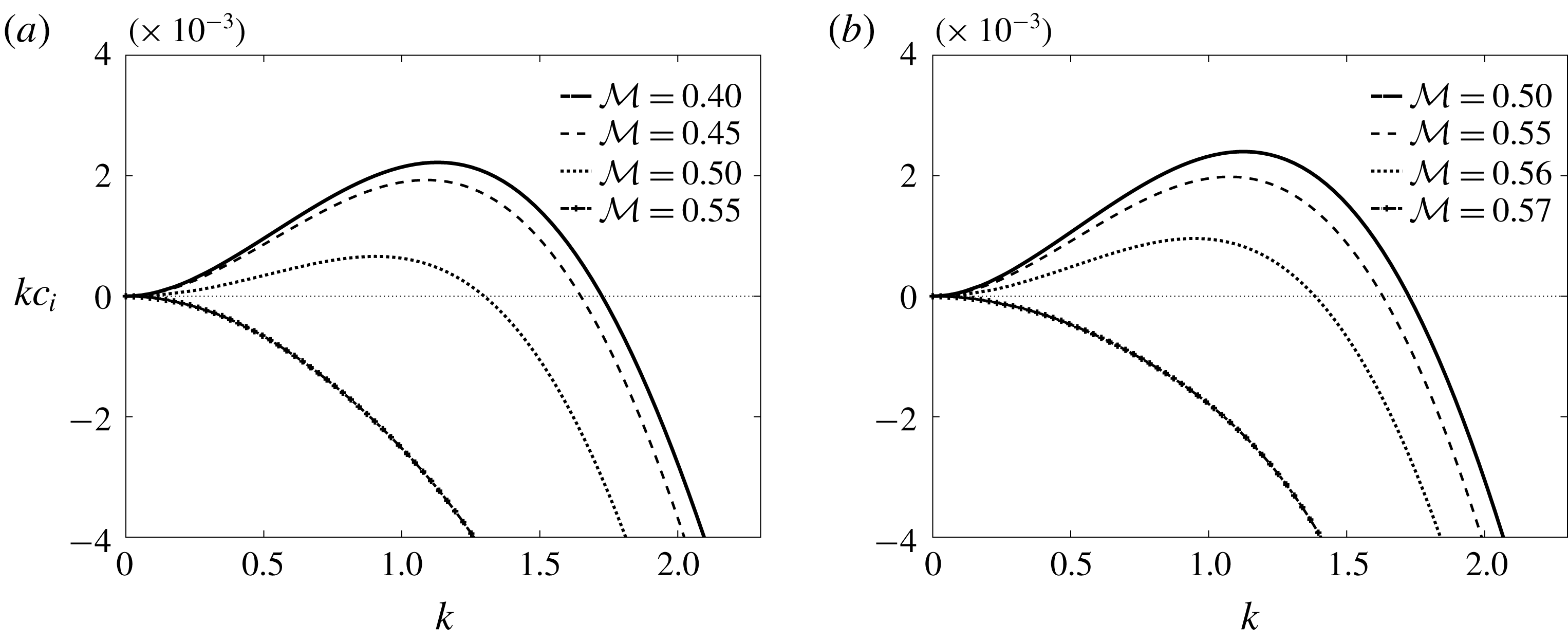
Figure 11 shows the dominant growth rates for various values of the surfactant mass, ${\mathcal{M}}$ , and for two different micelle sizes $N=10$ and $N=50$ (we also set $m=0.5$ , $n=10$ ). While the available mass is relatively small, we find that the growth rate curves are indistinguishable from the corresponding curves found in the absence of micelles; this is physically anticipated as at low mass availability the bulk concentration is small and below the CMC. For the chosen parametric set and $N=10$ , this is true for approximately ${\mathcal{M}}\leqslant 0.3$ . Increasing the mass diminishes the range of unstable wavenumbers and stabilises the system for ${\mathcal{M}}\geqslant 0.519$ (figure 11 a). When the preferred micelle size is larger at $N=50$ , more mass needs to be available to stabilise the interface, as shown in figure 11(b). The growth rate remains identical to the equivalent soluble one (obtained for $\tilde{M}=0$ ) up to ${\mathcal{M}}=0.4$ , but a rather rapid transition to stabilisation is seen as the surfactant mass increases to ${\mathcal{M}}=0.57$ . The final stable growth rate for large ${\mathcal{M}}$ is confirmed to be identical to the growth rate for a clean system without surfactant.

Figure 12.

Equilibrium surfactant concentrations $\bar{\unicode[STIX]{x1D6E4}}$ , $\bar{C}$ , $\bar{M}$ against available mass of surfactant ${\mathcal{M}}$ , found from (3.4) with $N=50$ , $h_{0}=1/11$ , $\unicode[STIX]{x1D6FD}_{b}=1$ , $K_{b}=1$ .

The latter observation is confirmed in figure 12 which illustrates the variation of surfactant concentrations $\bar{\unicode[STIX]{x1D6E4}}$ , $\bar{C}$ , $\bar{M}$ at equilibrium as functions of the total mass ${\mathcal{M}}$ , for micelle size $N=50$ . It is noteworthy that micelles only start to form for mass higher than approximately ${\mathcal{M}}=0.57$ , after which both $\bar{C}$ and $\bar{\unicode[STIX]{x1D6E4}}$ saturate to constant values while $\bar{M}$ keeps increasing (the saturated values are approximately $\bar{C}\rightarrow 1$ and $\bar{\unicode[STIX]{x1D6E4}}\rightarrow 0.5$ ). This implies that as soon as the micellisation starts, the adsorption and desorption processes are suspended, leaving the interface at a constant surface concentration while any additional mass causes the micelle concentration to grow (Burlatsky et al. Reference Burlatsky, Atrazhev, Dmitriev, Sultanov, Timokhina, Ugolkova, Tulyani and Vincitore2013). The stabilising action of micelles is physically associated with the plateau in the interfacial tension for bulk concentrations beyond the CMC (see figure 3), consequently the multi-layer Stokes flow is expected to be stable (similarly to the surfactant-free problem with constant surface tension).

In cases with $m\geqslant n^{2}$ , it is observed that the formation of micelles reduces the range of unstable wavenumbers and drives the growth rates towards zero; this is found to be true even for large values of mass ${\mathcal{M}}$ or micelle size $N$ (data not shown), and was corroborated using the long-wave asymptotic results.