1 Introduction
Coherent structures that span a broad range of length and time scales are common in wall-bounded turbulent flows (Cantwell Reference Cantwell1981; Robinson Reference Robinson1991; Adrian Reference Adrian2007; Jiménez Reference Jiménez2018). These structures play an important role in generating and sustaining turbulence. Near the wall, turbulence is self-sustaining through a regeneration process independent of the outer motions (Hamilton, Kim & Waleffe Reference Hamilton, Kim and Waleffe1995; Waleffe Reference Waleffe1997; Jiménez & Pinelli Reference Jiménez and Pinelli1999; Schoppa & Hussain Reference Schoppa and Hussain2002). In the logarithmic layer and the outer layer, there exist large-scale structures (Adrian Reference Adrian2007; Marusic et al. Reference Marusic, McKeon, Monkewitz, Nagib, Smits and Sreenivasan2010; Smits, McKeon & Marusic Reference Smits, McKeon and Marusic2011; Jiménez Reference Jiménez2018), which are further categorized into large-scale motions, hairpin packets (Kovasznay, Kibens & Blackwelder Reference Kovasznay, Kibens and Blackwelder1970; Brown & Thomas Reference Brown and Thomas1977; Adrian, Meinhart & Tomkins Reference Adrian, Meinhart and Tomkins2000; Ganapathisubramani, Longmire & Marusic Reference Ganapathisubramani, Longmire and Marusic2003; Tomkins & Adrian Reference Tomkins and Adrian2003; Deng et al. Reference Deng, Pan, Wang and He2018; Wang et al. Reference Wang, Gao, Wang, Wang and Pan2019), very-large-scale motions, superstructures (Kim & Adrian Reference Kim and Adrian1999; Guala, Hommema & Adrian Reference Guala, Hommema and Adrian2006; Balakumar & Adrian Reference Balakumar and Adrian2007; Hutchins & Marusic Reference Hutchins and Marusic2007; Lee & Sung Reference Lee and Sung2011; Wang & Zheng Reference Wang and Zheng2016), etc. These outer motions superimpose on top of and modulate the small-scale inner motions (Rao, Narasimha & Narayanan Reference Rao, Narasimha and Narayanan1971; Bandyopadhyay & Hussain Reference Bandyopadhyay and Hussain1984; Abe, Kawamura & Choi Reference Abe, Kawamura and Choi2004; Hutchins & Marusic Reference Hutchins and Marusic2007; Mathis, Hutchins & Marusic Reference Mathis, Hutchins and Marusic2009; Chung & McKeon Reference Chung and McKeon2010; Ganapathisubramani et al. Reference Ganapathisubramani, Hutchins, Monty, Chung and Marusic2012; Dogan et al. Reference Dogan, Örlü, Gatti, Vinuesa and Schlatter2019).
A general objective of turbulence modelling is to understand the statistical behaviours of the coherent motions in the flow. A well-studied phenomenological model is Townsend’s attached eddy hypothesis (AEH). The AEH was proposed by Townsend (Reference Townsend1976) and has received much attention in the recent literature. According to the AEH, the logarithmic layer may be modelled as an assembly of geometrically self-similar and statistically independent eddies that are attached to the wall. Following the AEH to its logical conclusions, the streamwise and spanwise velocity variances are logarithmic functions of the wall-normal distance  $y$ (Townsend Reference Townsend1976), and the wall-normal velocity variance is a constant, i.e.
 $$\begin{eqnarray}\left.\begin{array}{@{}c@{}}\displaystyle \langle u^{2+}\rangle =B_{1}-A_{1}\ln (\,y/\unicode[STIX]{x1D6FF}),\\ \displaystyle \langle w^{2+}\rangle =B_{3}-A_{3}\ln (\,y/\unicode[STIX]{x1D6FF}),\\ \displaystyle \langle v^{2+}\rangle =B_{2},\end{array}\right\}\end{eqnarray}$$
where  $u$,
 $v$ and
 $w$ are the streamwise, wall-normal and spanwise velocity fluctuations and the superscript
 $+$ denotes normalization by the friction velocity
 $u_{\unicode[STIX]{x1D70F}}=\sqrt{\unicode[STIX]{x1D70F}_{w}/\unicode[STIX]{x1D70C}}$ and the kinematic viscosity
 $\unicode[STIX]{x1D708}$. Here
 $\unicode[STIX]{x1D70F}_{w}$ is the wall-shear stress,
 $\unicode[STIX]{x1D70C}$ is the fluid density,
 $\unicode[STIX]{x1D6FF}$ is the outer length scale, i.e. boundary layer thickness, half-channel height or pipe radius, and
 $A_{1}$,
 $A_{3}$ and
 $B_{1,2,3}$ are constants. Empirical evidence of (1.1) was not found until quite recently when high-Reynolds-number data became available (Jiménez & Hoyas Reference Jiménez and Hoyas2008; Hultmark et al. Reference Hultmark, Vallikivi, Bailey and Smits2012; Marusic et al. Reference Marusic, Monty, Hultmark and Smits2013; Yamamoto & Tsuji Reference Yamamoto and Tsuji2018). In addition to the scalings in (1.1), several other scalings were identified by studying the AEH. These scalings include the logarithmic law of even-order moments (Meneveau & Marusic Reference Meneveau and Marusic2013), the power law of moment-generating functions (Yang, Marusic & Meneveau Reference Yang, Marusic and Meneveau2016b), the logarithmic law of two-point correlations (Yang, Marusic & Meneveau Reference Yang, Marusic and Meneveau2016a; Mouri Reference Mouri2017), the logarithmic law of two-point structure functions (Davidson, Nickels & Krogstad Reference Davidson, Nickels and Krogstad2006; De Silva et al. Reference De Silva, Marusic, Woodcock and Meneveau2015; Yang et al. Reference Yang, Baidya, Johnson, Marusic and Meneveau2017) as well as the velocity probability distribution scaling (Ge, Yang & Marusic Reference Ge, Yang and Marusic2019). On the one hand, the presence of these scalings shows the predictive power of the AEH; on the other hand, these scaling can be used to test if the extracted eddies are indeed attached eddies.
Despite the success of the AEH in providing scaling estimates of flow statistics in the logarithmic range, extracting attached eddies, or extracting the part of the velocity field from a flow that is due to attached eddies, is not very straightforward. Depending on the specific criterion to which one resorts, e.g. self-similarity, wall-attachedness, one could get different eddy structures. Del Álamo et al. (Reference Del Álamo, Jiménez, Zandonade and Moser2006) and Lozano-Durán, Flores & Jiménez (Reference Lozano-Durán, Flores and Jiménez2012) identified three-dimensional vortex clusters and quadrant structures that are geometrically self-similar. Hwang & Sung (Reference Hwang and Sung2018) extracted structures that lead to a logarithmic scaling of  $\langle u^{2}\rangle$. Hwang (Reference Hwang2015) isolated wall-attached eddies at a given spanwise length scale. Sharma & McKeon (Reference Sharma and McKeon2013) were able to find wall-attached modes in the framework of resolvent analysis (McKeon & Sharma Reference McKeon and Sharma2010). Hellström, Marusic & Smits (Reference Hellström, Marusic and Smits2016) observed self-similar wall-attached modes from their proper orthogonal decomposition analysis of turbulent pipe flows. Recently, Cheng et al. (Reference Cheng, Li, Lozano-Duran and Liu2019) adopted bidimensional empirical mode decomposition and argued that the third mode corresponds to attached eddies. A shortfall of the above methodologies is that the objective was to identify specific eddies and not to identify a part of the flow whose statistical behaviours are captured by the AEH. In a recent review, Marusic & Monty (Reference Marusic and Monty2019) pointed out that ‘attached eddies are only statistically representative structures and searching for candidate attached eddy shapes from flow visualizations is highly problematic and potentially misleading’. In this work, we will follow Marusic & Monty (Reference Marusic and Monty2019) and focus on extracting the part of the flow whose statistical properties are captured by the AEH.
While the data support the AEH in general, there are definite inconsistencies between the AEH and the data. First, the logarithmic law of the wall is a good working approximation of the mean flow at moderate Reynolds numbers from about  $y^{+}=30$ to about
 $y/\unicode[STIX]{x1D6FF}=0.2$ (Jiménez & Moser Reference Jiménez and Moser2007; Lee & Moser Reference Lee and Moser2015), but the logarithmic law of the streamwise velocity variance, which should be a good working approximation of
 $\langle u^{2}\rangle$ in the same wall-normal distance range at the same Reynolds-number range as the logarithmic law of the wall, is valid only at high Reynolds numbers and in a comparably much more limited wall-normal distance range (Marusic et al. Reference Marusic, Monty, Hultmark and Smits2013; Yamamoto & Tsuji Reference Yamamoto and Tsuji2018). Second, according to the AEH, the attached eddies are Gaussian, but the streamwise flow statistics are in reality sub-Gaussian (Meneveau & Marusic Reference Meneveau and Marusic2013; Woodcock & Marusic Reference Woodcock and Marusic2015; Yang et al. Reference Yang, Marusic and Meneveau2016b). Hence it is safe to say that, in addition to attached eddies and small-scale isotropic eddies, there are other types of energy-containing eddies in the flow.
Admitting that the AEH is not a complete description of wall-bounded flows, some studies have attempted to model eddies that are not wall-attached. Perry & Marusic (Reference Perry and Marusic1995) refined the attached eddy model by incorporating two types of eddies, i.e. type-A and type-B eddies. Type-A eddies are ‘wall structures’ (wall-attached eddies) and type-B eddies are ‘wake structures’ (wall-detached eddies). There is also a small amount of turbulence kinetic energy from type-C eddies, which are Kolmogorov-scale eddies (Perry, Henbest & Chong Reference Perry, Henbest and Chong1986; Perry & Marusic Reference Perry and Marusic1995). Recently, Baars & Marusic (Reference Baars and Marusic2020a) proposed a data-based spectral decomposition method. They followed Perry & Marusic (Reference Perry and Marusic1995) and separated the type-A and type-B eddies using two continuous spectral filters. A log-linear scaling of  $\langle u^{2+}\rangle$ with a Townsend–Perry constant of
 $A_{1}=0.98$ was found, suggesting that type-A eddies might be wall-attached eddies as described in the AEH (Baars & Marusic Reference Baars and Marusic2020b).
The present study shares a similar objective to that of Baars & Marusic (Reference Baars and Marusic2020a,Reference Baars and Marusicb) and Perry & Marusic (Reference Perry and Marusic1995), but as will become clear in the later sections, we take a statistical perspective and our discussion is more closely linked to Townsend (Reference Townsend1976). We decompose the flow field into ‘wall-attached eddies’, ‘wall-detached eddies’ and Kolmogorov-scale eddies. We show that the statistical behaviours of the extracted wall-attached eddies are well described by the AEH. Then, we study the statistical properties of the wall-detached eddies, whose statistical behaviours are not captured by the AEH. Last we study the interaction among the small-scale eddies, the wall-attached eddies and the wall-detached eddies. Recently, Lee & Moser (Reference Lee and Moser2019) decomposed the streamwise velocity by applying a spectral filter that cuts off at  $\unicode[STIX]{x1D706}^{+}=1000$, and studied the interaction between the large and the small scales. They found that the large scales project turbulence energy into the near-wall region and control the small scales, which we verify in our work.
The rest of the paper is organized as follows. Details of the dataset are presented in § 2 along with the decomposition methodology. In § 3, we show that the statistical properties of the extracted part of the flow are captured by the AEH. We study the properties of the detached eddies in § 4, where a phenomenological model for the detached eddies is proposed. Then, we study the interactions between the attached eddies and the detached eddies in § 5. We show the instantaneous flow fields of each type of eddy in § 6, and in § 7 we present our conclusions. Throughout this paper, we use  $x$,
 $y$ and
 $z$ to denote the streamwise, wall-normal and spanwise directions, fluctuating velocity components are denoted using lowercase letters, e.g.
 $u$ is the streamwise velocity fluctuation, and variables in wall units are denoted using superscript
 $+$.
2 Datasets and methodology
2.1 Dataset description
We use three sets of data, i.e. direct numerical simulations of turbulent channel flow (Lee & Moser Reference Lee and Moser2015), hot-wire measurements of zero-pressure-gradient turbulent boundary layers (ZPGTBLs) (Hutchins et al. Reference Hutchins, Nickels, Marusic and Chong2009; Philip et al. Reference Philip, Baidya, Hutchins, Monty and Marusic2013; Baars et al. Reference Baars, Talluru, Hutchins and Marusic2015; Marusic et al. Reference Marusic, Chauhan, Kulandaivelu and Hutchins2015; Baidya Reference Baidya2016) and field measurements of an atmospheric surface layer (ASL) (Wang & Zheng Reference Wang and Zheng2016).
The direct numerical simulations solve the incompressible Navier–Stokes equations in a periodic channel (Lee, Malaya & Moser Reference Lee, Malaya and Moser2013). The computation domain is  $8\unicode[STIX]{x03C0}\times 2\times 3\unicode[STIX]{x03C0}$ in the streamwise (
 $x$), wall-normal (
 $y$) and spanwise (
 $z$) directions, respectively. The half-channel height is unity. The friction Reynolds numbers of the direct numerical simulations are
 $Re_{\unicode[STIX]{x1D70F}}\approx$ 1000, 2000 and 5200. The dataset is maintained by the University of Texas at Austin, and the data at
 $Re_{\unicode[STIX]{x1D70F}}\approx 1000$ and 5200 can be accessed through the Johns Hopkins Turbulence Database (http://turbulence.pha.jhu.edu/) (Graham et al. Reference Graham, Kanov, Yang, Lee, Malaya, Lalescu, Burns, Eyink, Szalay and Moser2016).
The ZPGTBL data are hot-wire measurements in the High Reynolds Number Boundary Layer Wind Tunnel at the University of Melbourne (Hutchins et al. Reference Hutchins, Nickels, Marusic and Chong2009; Marusic et al. Reference Marusic, Chauhan, Kulandaivelu and Hutchins2015). The wind tunnel has a test section of 27 m. The Reynolds numbers are from  $Re_{\unicode[STIX]{x1D70F}}\approx 2800$ to 13 000. We also adopt data of two-point synchronous hot-wire measurement at
 $Re_{\unicode[STIX]{x1D70F}}\approx 15\,000$ (Baars et al. Reference Baars, Talluru, Hutchins and Marusic2015; Baars, Hutchins & Marusic Reference Baars, Hutchins and Marusic2017) and the
 $x$-wire measurements of ZPGTBL flow at
 $Re_{\unicode[STIX]{x1D70F}}\approx 10\,000$ (Philip et al. Reference Philip, Baidya, Hutchins, Monty and Marusic2013; Baidya Reference Baidya2016). The sampling rate is 20 kHz and the non-dimensional sampling interval is
 $\unicode[STIX]{x0394}T^{+}\approx 1.3$. The measurement lasted for about
 $TU_{\infty }/\unicode[STIX]{x1D6FF}=20\,000$.
The ASL data are field measurements at the Qingtu Lake Observation Array (QLOA) site in western China under near-neutral atmospheric stratification conditions (Wang & Zheng Reference Wang and Zheng2016). The Reynolds number is as high as  $Re_{\unicode[STIX]{x1D70F}}\sim O(10^{6})$. Sonic anemometers (Gill Instruments R3-50 and Campbell CSAT3B) were installed to record the three velocity components at a sampling rate of 50 Hz. The raw data are split into multiple one-hour segments for subsequent analysis, and the non-dimensional time duration of each segment is
 $TU_{\infty }/\unicode[STIX]{x1D6FF}=200$–
 $400$, during which the flow is roughly statistically stationary.
2.2 A decomposition scheme
Following the discussion in the introduction, it is known that not all the eddies are wall-attached. In this section, we propose a decomposition scheme that extracts the velocity induced by wall-attached eddies. The scheme follows directly from Townsend (Reference Townsend1976). The objective is to extract the part of the velocity field that is due to wall-attached eddies (rather than to extract specific eddies that are wall-attached). According to Townsend (Reference Townsend1976): first, sizes of wall-attached eddies scale as their distances from the wall; second, the streamwise and the spanwise velocities at a distance from the wall are a superposition of eddy-induced velocities; third, at a distance from the wall, the wall-normal velocity component is solely due to the attached eddy at that distance because of the wall blocking effect. These three statements are discussed in further detail in, for example, Perry & Chong (Reference Perry and Chong1982), Meneveau & Marusic (Reference Meneveau and Marusic2013) and Yang & Meneveau (Reference Yang and Meneveau2019). It follows from the three statements that attached eddies are responsible for the streamwise and spanwise velocities of scale
 $$\begin{eqnarray}\unicode[STIX]{x1D6FC}_{1,3}y<\unicode[STIX]{x1D706}_{x}<\unicode[STIX]{x1D6FD}_{1,3}\unicode[STIX]{x1D6FF},\quad \unicode[STIX]{x1D6FE}_{1,3}<y^{+},\end{eqnarray}$$
where  $\unicode[STIX]{x1D6FC}$,
 $\unicode[STIX]{x1D6FD}$ and
 $\unicode[STIX]{x1D6FE}$ are constants, and the subscripts
 $1$ and
 $3$ denote the streamwise and the spanwise velocity components. Because attached eddies are not isotropic flow structures,
 $\unicode[STIX]{x1D6FC}_{1}$,
 $\unicode[STIX]{x1D6FD}_{1}$ and
 $\unicode[STIX]{x1D6FE}_{1}$ are not necessarily equal to
 $\unicode[STIX]{x1D6FC}_{3}$,
 $\unicode[STIX]{x1D6FD}_{3}$ and
 $\unicode[STIX]{x1D6FE}_{3}$. The constant
 $\unicode[STIX]{x1D6FE}$ is a viscous cutoff, the lower limit
 $\unicode[STIX]{x1D6FC}y$ scales with
 $y$ because attached eddies scale with their distances from the wall and the upper limit scales with
 $\unicode[STIX]{x1D6FF}$ because the largest eddies, which scale with
 $\unicode[STIX]{x1D6FF}$, also contribute to the streamwise velocity at
 $y$. For the wall-normal velocity component, the attached eddies are responsible for the scales
 $$\begin{eqnarray}\unicode[STIX]{x1D6FC}_{2}y<\unicode[STIX]{x1D706}_{x}<\unicode[STIX]{x1D6FD}_{2}y,\quad \unicode[STIX]{x1D6FE}_{2}<y^{+}.\end{eqnarray}$$
The upper limit scales with  $y$ instead of
 $\unicode[STIX]{x1D6FF}$ because the larger scales do not contribute to the local wall-normal velocity.
The velocities of scales in (2.1) and (2.2) are due to wall-attached eddies. This means that a subset of these scales are also induced by wall-attached eddies. A direct implication is that, if a set of constants, i.e.  $\unicode[STIX]{x1D6FC}_{1,2,3}$,
 $\unicode[STIX]{x1D6FD}_{1,2,3}$ and
 $\unicode[STIX]{x1D6FE}_{1,2,3}$, are appropriate for extracting attached eddy-induced flow fields, any
 $\unicode[STIX]{x1D6FC}_{1,2,3}^{\prime }$,
 $\unicode[STIX]{x1D6FD}_{1,2,3}^{\prime }$ and
 $\unicode[STIX]{x1D6FE}_{1,2,3}^{\prime }$ such that
 $$\begin{eqnarray}\unicode[STIX]{x1D6FE}_{1,2,3}^{\prime }>\unicode[STIX]{x1D6FE}_{1,2,3},\quad \unicode[STIX]{x1D6FC}_{1,2,3}^{\prime }>\unicode[STIX]{x1D6FC}_{1,2,3},\quad \unicode[STIX]{x1D6FD}_{1,2,3}^{\prime }<\unicode[STIX]{x1D6FD}_{1,2,3}\end{eqnarray}$$
will also be appropriate for extracting attached eddy-induced flow fields. It is only if we use  $\unicode[STIX]{x1D6FC}_{1,2,3}^{\prime }$,
 $\unicode[STIX]{x1D6FD}_{1,2,3}^{\prime }$ and
 $\unicode[STIX]{x1D6FE}_{1,2,3}^{\prime }$ instead of
 $\unicode[STIX]{x1D6FC}_{1,2,3}$,
 $\unicode[STIX]{x1D6FD}_{1,2,3}$ and
 $\unicode[STIX]{x1D6FE}_{1,2,3}$ that some scales that could have been included as attached eddies would be precluded.
2.3 The pre-multiplied velocity spectra of wall-attached eddies
Following the discussion in the previous section, although we could be conservative in choosing the constants, the idea is to find  $\unicode[STIX]{x1D6FC}_{1,2,3}$,
 $\unicode[STIX]{x1D6FD}_{1,2,3}$ and
 $\unicode[STIX]{x1D6FE}_{1,2,3}$ such that as many scales as possible are included in (2.1) and (2.2). Because our scheme in § 2.2 is a scale decomposition one, it is most natural to start our discussion from the velocity spectra. The spectrum of a single wall-attached eddy is the topic of, for example, Baidya et al. (Reference Baidya, Philip, Hutchins, Monty and Marusic2017). Nonetheless, not too much is known about the spectrum of an assembly of wall-attached eddies. In the following, we will derive the velocity spectra due to an assembly of wall-attached eddies.
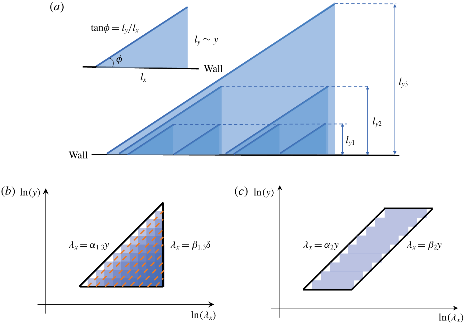
In figure 1(a), we sketch three hierarchies of attached eddies. Here, the inclination angle is  $\unicode[STIX]{x1D719}$. The geometric representation in figure 1(a) is not meant to be taken literally. In general,
 $\tan \unicode[STIX]{x1D719}=l_{y}/l_{x}\approx y/l_{x}$ and
 $l_{x}\approx y/\tan \unicode[STIX]{x1D719}$, where
 $l_{y}$ is the eddy height and
 $l_{x}$ is the streamwise extent of the eddy. Note that
 $y/l_{x}$ could also be regarded as the wall/normal-streamwise aspect ratio of attached eddies. The corresponding pre-multiplied streamwise (spanwise) velocity energy spectrum
 $k_{x}E_{uu}$ (
 $k_{x}E_{ww}$) is sketched in figure 1(b), where
 $k_{x}$ is the streamwise wavenumber and
 $E_{uu}$ (
 $E_{ww}$) is the streamwise (spanwise) energy spectrum. In the following, our discussion will focus on the streamwise velocity component with the understanding that a similar argument applies to the spanwise velocity component. Eddies of height
 $y$ contribute to the pre-multiplied spectrum in
 $\unicode[STIX]{x1D6FC}_{1}y<\unicode[STIX]{x1D706}_{x}<\unicode[STIX]{x1D6FD}_{1}\unicode[STIX]{x1D6FF}$,
 $\unicode[STIX]{x1D6FE}_{1}<y^{+}$ and
 $y<l_{y}$, where
 $\unicode[STIX]{x1D6FD}_{1}\unicode[STIX]{x1D6FF}$ and
 $\unicode[STIX]{x1D6FC}_{1}y$ are the largest and the smallest streamwise (spanwise) velocity length scale at height
 $l_{y}=y$, and
 $\unicode[STIX]{x1D6FE}_{1}\approx 100$ is the viscous cutoff (Perry & Chong Reference Perry and Chong1982). Adding contributions from all wall-attached eddies, the attached eddies are responsible for the region enclosed by the triangle in figure 1(b), in which region the scaling of the contour levels is
 $\unicode[STIX]{x1D706}_{x}\sim y$. Baars, Hutchins & Marusic (Reference Baars, Hutchins and Marusic2017) carried out a similar analysis for the spectral coherence spectrum. In the context of this work, it is more straightforward to do this analysis for the pre-multiplied energy spectra, the integration of which leads to the kinetic energy. Next, let us derive the pre-multiplied wall-normal velocity spectrum. This is comparably simpler because the local wall-normal velocity is solely controlled by the local wall-attached eddies (Townsend Reference Townsend1976; Perry & Chong Reference Perry and Chong1982; Yang et al. Reference Yang, Baidya, Lv and Marusic2018). Figure 1(c) shows the pre-multiplied wall-normal velocity spectrum, where there is no superposition of contributions from eddies of different sizes.
(a) Sketch of three hierarchies of wall-attached eddies. A typical attached eddy is also sketched. (b) The resulting pre-multiplied spectrum of the streamwise/ spanwise velocity due to nine hierarchies of attached eddies. (c) The resulting pre-multiplied spectrum of the wall-normal velocity due to nine hierarchies of attached eddies.

2.4 The velocity spectrum
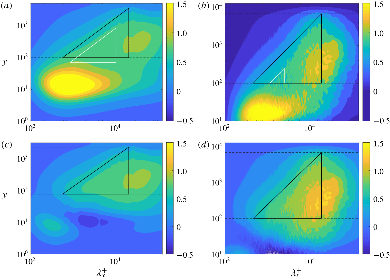
There is no guarantee that the spectral behaviour derived above could be found in reality. In this subsection, we take a look at the measured pre-multiplied velocity spectra, and see if figure 1 is consistent with the data. We show  $k_{x}E_{uu}^{+}$ in a
 $Re_{\unicode[STIX]{x1D70F}}=5200$ channel and a
 $Re_{\unicode[STIX]{x1D70F}}=13\,000$ ZPGTBL in figures 2(a) and 2(b), respectively. Removing the inner-scale motions according to Hu & Zheng (Reference Hu and Zheng2018), the remaining parts of the spectra are shown in figure 2(c,d). The regions enclosed in the black triangles exhibit the predicted behaviour, and, according to our discussion in the previous subsection, these regions represent velocities due to wall-attached eddies.
Pre-multiplied streamwise velocity spectra in (a) a  $Re_{\unicode[STIX]{x1D70F}}=5200$ channel and (b) a
 $Re_{\unicode[STIX]{x1D70F}}=13\,000$ ZPGTBL, and spectra with the inner scales removed in (c) a
 $Re_{\unicode[STIX]{x1D70F}}=5200$ channel and (d) a
 $Re_{\unicode[STIX]{x1D70F}}=13\,000$ ZPGTBL. The thin dashed lines are at the viscous cutoff
 $y^{+}=100$ and the height of the largest attached eddies. The white triangle in (a) corresponds to (2.5) and that in (b) corresponds to (2.4). The black triangles are the present decomposition scheme.

An extensively studied scaling is the  $k_{x}^{-1}$ law of the streamwise velocity spectrum (Perry & Chong Reference Perry and Chong1982; Perry et al. Reference Perry, Henbest and Chong1986), based on which one could also claim a region in the velocity spectrum that represents contributions from wall-attached eddies. These regions are similar to ours in that they enclose a triangular region of the velocity spectrum, although these studies did not make a connection between this triangular region and the behaviour of
 $\langle u^{2}\rangle$. For instance, Nickels et al. (Reference Nickels, Marusic, Hafez and Chong2005) proposed the following region for boundary layers:
 $$\begin{eqnarray}y^{+}>100,\quad \unicode[STIX]{x1D706}_{x}\geqslant 15.7y\quad \text{and}\quad \unicode[STIX]{x1D706}_{x}\leqslant 0.3\unicode[STIX]{x1D6FF},\end{eqnarray}$$
and Hwang (Reference Hwang2015) proposed
 $$\begin{eqnarray}y^{+}>70,\quad \unicode[STIX]{x1D706}_{x}\geqslant 12y\quad \text{and}\quad \unicode[STIX]{x1D706}_{x}\leqslant 2\unicode[STIX]{x1D6FF}\end{eqnarray}$$
for a channel, both of which are shown in figure 2. Depending on the flow quantity at which one looks, the definition of the logarithmic layer, or the scales that are relevant to the logarithmic layer, could be very different. For example, if one looks at the mean flow, one may claim that the logarithmic layer is from  $y^{+}=30$ to
 $y/\unicode[STIX]{x1D6FF}=0.2$, but if one looks at the streamwise velocity variance, one may argue that the logarithmic layer is from
 $y^{+}=3\sqrt{Re_{\unicode[STIX]{x1D70F}}}$ to
 $y/\unicode[STIX]{x1D6FF}=0.15$ (Marusic et al. Reference Marusic, Monty, Hultmark and Smits2013). Compared to the scalings we look at in this work, i.e. the
 $y\sim \unicode[STIX]{x1D706}_{x}$ scaling of the pre-multiplied velocity spectrum, the
 $k^{-1}$ scaling is much more difficult to find (Mouri, Morinaga & Haginoya Reference Mouri, Morinaga and Haginoya2019). Hence, although Hwang (Reference Hwang2015), Nickels et al. (Reference Nickels, Marusic, Hafez and Chong2005) and we are looking for the parts of the velocity spectrum that represent contributions from wall-attached eddies, the claimed regions in Hwang (Reference Hwang2015) and Nickels et al. (Reference Nickels, Marusic, Hafez and Chong2005) and by us will be different.
The remaining parts of the streamwise velocity spectrum, i.e. the parts outside the triangle, are not due to wall-attached eddies. The small-scale eddies, i.e.  $\unicode[STIX]{x1D706}_{x}<\unicode[STIX]{x1D6FC}_{1}y$, are roughly isotropic. Their contributions to the turbulent kinetic energy are usually small at high Reynolds numbers. The larger-scale motions, i.e.
 $\unicode[STIX]{x1D706}_{x}>\unicode[STIX]{x1D6FD}_{1}\unicode[STIX]{x1D6FF}$ in the pre-multiplied spectrum, contribute significantly to the turbulent kinetic energy. For reasons that will be clear in a later section, we will refer to the motions that are responsible for the region
 $\unicode[STIX]{x1D706}_{x}>\unicode[STIX]{x1D6FD}_{1}\unicode[STIX]{x1D6FF}$ in the pre-multiplied spectrum as ‘detached eddies’.
We make a note about the connections and the differences between the present definitions and those in the literature. The type-A eddies in Perry & Marusic (Reference Perry and Marusic1995) are attached eddies. The type-B and type-C eddies are similar to the detached eddies and the small-scale eddies defined herein. The ‘detached eddies’ in Perry & Marusic (Reference Perry and Marusic1995), Katul & Vidakovic (Reference Katul and Vidakovic1996), Jiménez (Reference Jiménez2012) and Agostini & Leschziner (Reference Agostini and Leschziner2017) are Kolmogorov-scale eddies similar to our small-scale eddies.
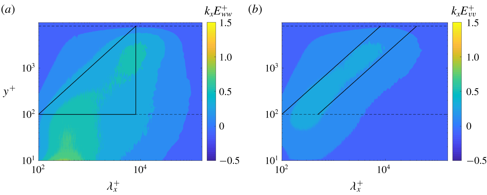
Having looked at the streamwise velocity spectrum, we take a look at the spanwise and the wall-normal velocity spectra. The pre-multiplied spanwise and wall-normal velocity spectra are shown in figures 3(a) and 3(b), respectively, in a  $Re_{\unicode[STIX]{x1D70F}}\approx 10\,000$ ZPGTBL. The predicted behaviours are found in the triangular region (2.1) and parallelogram region (2.2).
Pre-multiplied spectra of the transverse velocity components in ZPGTBL flow at  $Re_{\unicode[STIX]{x1D70F}}\approx 10\,000$: (a) the spanwise velocity; (b) the wall-normal velocity.

2.5 Constants in the decomposition
To extract the wall-attached motions, we need to determine the constants in (2.1) and (2.2). Following the discussion in § 2.2, we could be conservative and leave out some of the attached eddies, but here we hope to include all the scales that represent contributions from attached eddies. Per figure 2,  $\unicode[STIX]{x1D6FC}_{1}=5.7$ and
 $\unicode[STIX]{x1D6FE}_{1}=100$. The viscous cutoff is
 $\unicode[STIX]{x1D6FE}_{1}=100$ as follows from Perry & Chong (Reference Perry and Chong1982). The small-scale cutoff follows from the inclination angle of streamwise velocity signals, i.e.
 $\unicode[STIX]{x1D6FC}_{1}=1/\tan (\unicode[STIX]{x1D719}_{1})$, where
 $\unicode[STIX]{x1D719}_{1}\approx 10^{\circ }$ is the inclination angle of streamwise velocity signals (Brown & Thomas Reference Brown and Thomas1977; Adrian et al. Reference Adrian, Meinhart and Tomkins2000; Christensen & Adrian Reference Christensen and Adrian2001; Marusic & Heuer Reference Marusic and Heuer2007; De Silva, Hutchins & Marusic Reference De Silva, Hutchins and Marusic2016; Liu, Bo & Liang Reference Liu, Bo and Liang2017). The large-scale cutoff is
 $\unicode[STIX]{x1D6FD}_{1}=3$ for boundary layer and
 $\unicode[STIX]{x1D6FD}_{1}=4$ for channel, considering that the large scales in channel are longer than those in boundary layer (Monty et al. Reference Monty, Hutchins, Ng, Marusic and Chong2009). If the same, more conservative constant
 $\unicode[STIX]{x1D6FD}_{1}=3$ is used for both channel and boundary layer, the extracted part of the flow would still be due to wall-attached eddies, but we will miss scales that should have been included in the context of channel flow. Per figure 3,
 $\unicode[STIX]{x1D6FE}_{2,3}=100$,
 $\unicode[STIX]{x1D6FC}_{2,3}=1$,
 $\unicode[STIX]{x1D6FD}_{3}=1$ and
 $\unicode[STIX]{x1D6FD}_{2}=5$. The viscous cutoff for the spanwise and the wall-normal velocity is the same as that for the streamwise velocity. The longitudinal scales of the spanwise and wall-normal velocity components are smaller than the streamwise component (Del Álamo et al. Reference Del Álamo, Jiménez, Zandonade and Moser2004; Jiménez & Hoyas Reference Jiménez and Hoyas2008; Hwang Reference Hwang2015; Hwang & Sung Reference Hwang and Sung2018; Yang & Bo Reference Yang and Bo2018; Cheng et al. Reference Cheng, Li, Lozano-Duran and Liu2019), and hence
 $\unicode[STIX]{x1D6FC}_{2,3}<\unicode[STIX]{x1D6FC}_{1}$. The specific value
 $\unicode[STIX]{x1D6FC}_{2,3}=1$ corresponds to a
 $45^{\circ }$ inclination angle of spanwise and wall-normal velocity signals (Head & Bandyopadhyay Reference Head and Bandyopadhyay1981). According to our discussion in 2.2, the AEH should provide a complete statistical description of the scales in these regions.
3 Wall-attached eddies
In § 2.4, we showed that the AEH is able to predict the behaviour of the pre-multiplied velocity spectrum in the enclosed regions in figures 2 and 3. If the AEH is valid, by applying the spectral decomposition (2.1) to the datasets in § 2.1, we should be able to extract the part of the flow whose statistical properties (including the behaviour of the velocity spectrum but also the behaviour of other statistical flow quantities) are captured by the AEH. In this section, we will carefully test if this is true by comparing statistical properties of the extracted eddies to the predictions of the AEH. We will be able to conclude that the AEH is a good model for the extracted part of the flow if the statistical properties of the extracted scales are captured by the AEH. In the following, we focus on the streamwise velocity component and also show results for the spanwise and the wall-normal velocity components.
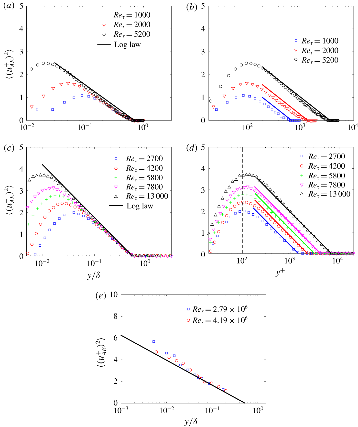
Streamwise velocity variances of the attached eddies in turbulent channel flow (a,b), ZPGTBL flow (c,d) and ASL flow (e). The solid lines correspond to (3.2a.b), with  $C_{1}=0.8$ for turbulent channel flows, and
 $C_{1}=1.0$ for ZPGTBL flows and ASL flows.

3.1 Velocity variances
The logarithmic variation of the streamwise velocity variance is probably the most well-known consequence of the AEH (Townsend Reference Townsend1976):
 $$\begin{eqnarray}\left\langle (u_{AE}^{+})^{2}\right\rangle =D_{1}-C_{1}\ln (\,y/\unicode[STIX]{x1D6FF}).\end{eqnarray}$$
We can rewrite the above equation (3.1) as
 $$\begin{eqnarray}\left\langle (u_{AE}^{+})^{2}\right\rangle =C_{1}\ln (\unicode[STIX]{x1D6FF}_{i}/y),\quad \unicode[STIX]{x1D6FF}_{i}=(\unicode[STIX]{x1D6FD}_{1}/\unicode[STIX]{x1D6FC}_{1})\unicode[STIX]{x1D6FF},\end{eqnarray}$$
where  $\langle (u_{AE}^{+})^{2}\rangle =0$ at
 $y=\unicode[STIX]{x1D6FF}_{i}$. In previous literature, although the logarithmic scaling of the streamwise velocity variance was found, its wall-normal extent and the Reynolds number range of the scaling found are not entirely consistent with the AEH. Figure 4 shows the streamwise velocity variance of the attached eddies in turbulent channel flow, ZPGTBL and ASL. The Reynolds number spans about three decades, i.e.
 $Re_{\unicode[STIX]{x1D70F}}$ from
 $O(10^{3})$ to
 $O(10^{6})$. The logarithmic scaling of
 $\langle (u_{AE}^{+})^{2}\rangle$ starts at
 $y^{+}\sim O(10^{2})$, i.e. the viscous cutoff, and ends at
 $y=\unicode[STIX]{x1D6FF}_{i}$, following precisely the prediction of the AEH. The constant
 $C_{1}$ is 0.8 in channel flow and 1.0 in boundary layer flow. The measurement of Baars & Marusic (Reference Baars and Marusic2020b) shows that
 $C_{1}=0.98$ in boundary layer, which is very close to our measurement here. It is noted that the scaling of streamwise velocity variance was also considered by other approaches (Monkewitz & Nagib Reference Monkewitz and Nagib2015; Vassilicos et al. Reference Vassilicos, Laval, Foucaut and Stanislas2015; Laval et al. Reference Laval, Vassilicos, Foucaut and Stanislas2017; Chen, Hussain & She Reference Chen, Hussain and She2018).
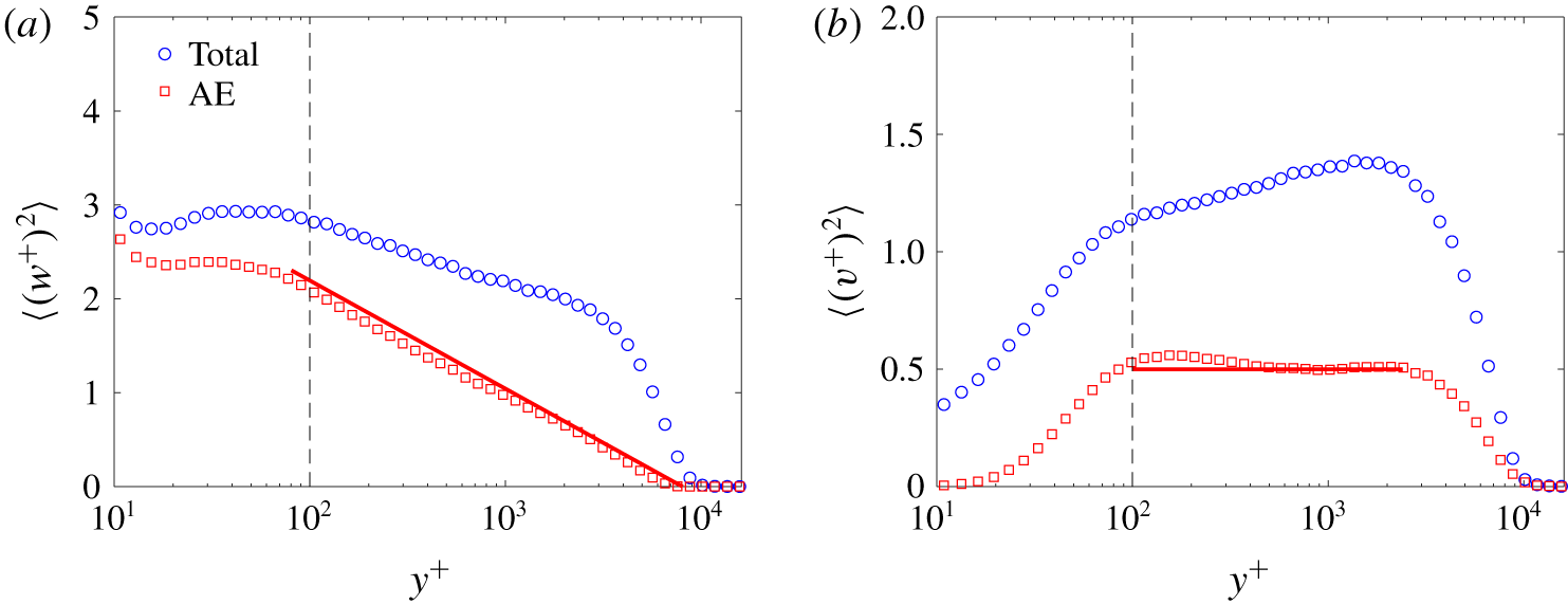
Figure 5 shows the spanwise and wall-normal velocity variances due to the attached eddies in a  $Re_{\unicode[STIX]{x1D70F}}=10\,000$ boundary layer. According to the AEH,
 $$\begin{eqnarray}\left\langle (w_{AE}^{+})^{2}\right\rangle =D_{3}-C_{3}\ln (\,y/\unicode[STIX]{x1D6FF}),\quad \left\langle (v_{AE}^{+})^{2}\right\rangle =D_{2},\end{eqnarray}$$
which are consistent with the data in figure 5.
Variances of transverse velocity components in ZPGTBL flow at  $Re_{\unicode[STIX]{x1D70F}}\approx 10\,000$: (a) spanwise velocity; (b) wall-normal velocity. The solid lines correspond to (3.3), with
 $C_{3}=0.5$ and
 $D_{2}=0.5$. AE, attached eddies.

Several recent studies reported similar results. Ganapathisubramani (Reference Ganapathisubramani2018) applied a high-pass frequency filter  $f^{+}=0.005$ to ZPGTBL measurement data and found a universal logarithmic law of the small-scale streamwise velocity variance. Lee & Moser (Reference Lee and Moser2019) applied a high-pass spectral filter
 $\unicode[STIX]{x1D706}^{+}=1000$ to turbulent channel flow data (Lee & Moser Reference Lee and Moser2015), and found a logarithmic scaling of the small-scale streamwise and spanwise velocity fluctuations. Nonetheless, because the extracted part of the flow in those two studies does not exactly correspond to the triangular region in figure 1(b), in principle, one could not claim that the observed scalings in those two studies are results of attached eddies, and because those two studies did not compare other statistical properties of the extracted eddies to the predictions of the AEH, one probably could not claim with confidence that the extracted eddies are the attached eddies as described in the AEH.
In order to claim that the extracted eddies are wall-attached eddies, every aspect of the statistical properties of the extracted eddies should be captured by the AEH. Next, we will take a look at other statistics.
3.2 High-even-order moments
Meneveau & Marusic (Reference Meneveau and Marusic2013) concluded from the AEH that high-even-order moments behave logarithmically as a function of the wall-normal distance:
 $$\begin{eqnarray}\langle (u^{+})^{2p}\rangle ^{1/p}=B_{1,p}-A_{1,p}\ln (\,y/\unicode[STIX]{x1D6FF}),\end{eqnarray}$$
where  $A_{1,p}=A_{1}[(2p-1)!!]^{1/p}$ because of the presumed Gaussianality of the wall-attached eddies,
 $n!!\equiv n(n-2)(n-4)\ldots 1$ is the double factorial and
 $A_{1}$ is the Townsend–Perry constant (Marusic et al. Reference Marusic, Monty, Hultmark and Smits2013). They argued that because the velocity increment due to each wall-attached eddy is identical and independent, the summation of these velocity increments is Gaussian as per the central limit theorem. This follows directly from Townsend, where he argued that all attached eddies are independent and the flow field is ‘homogeneous’ in terms of the appearance of wall-attached eddies. While the logarithmic scaling was found, the measured slopes
 $A_{p}$ are sub-Gaussian instead of Gaussian.
Following Meneveau & Marusic (Reference Meneveau and Marusic2013), for attached eddies, the even-order moments should follow
 $$\begin{eqnarray}\displaystyle & \displaystyle \langle (u_{AE}^{+})^{2p}\rangle ^{1/p}=C_{1,p}\ln (\unicode[STIX]{x1D6FF}_{i}/y), & \displaystyle\end{eqnarray}$$
 $$\begin{eqnarray}\displaystyle & \displaystyle \langle (w_{AE}^{+})^{2p}\rangle ^{1/p}=C_{3,p}\ln (\unicode[STIX]{x1D6FF}_{i}/y), & \displaystyle\end{eqnarray}$$
where  $C_{1,p}=C_{1}[(2p-1)!!]^{1/p}$ and
 $C_{3,p}=C_{3}[(2p-1)!!]^{1/p}$. We test if that is the case. We can claim success only if (i) the predicted scaling is found and (ii) the pre-factors are Gaussian.
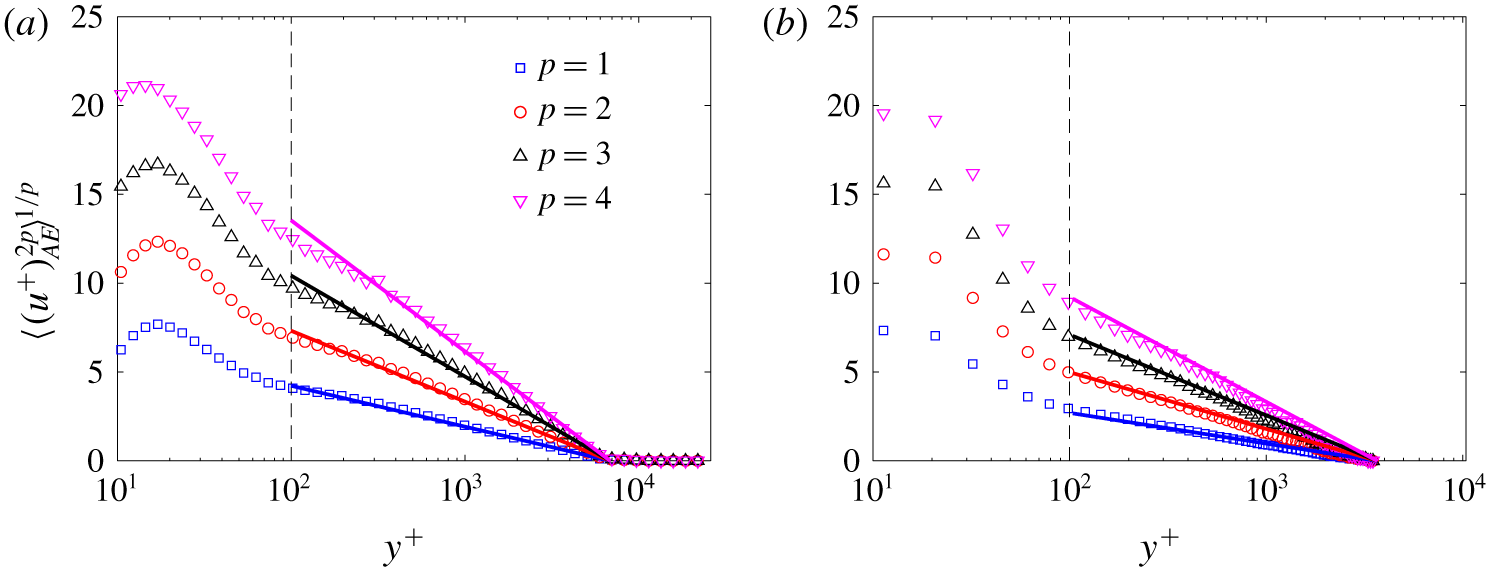
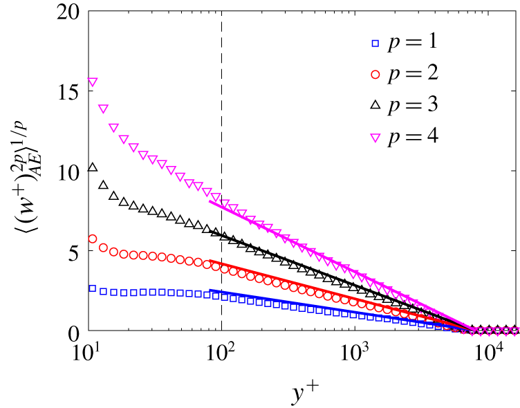
Figure 6 shows the high-even-order moments of streamwise velocity of the attached eddies for  $p=1,2,3,4$ in a ZPGTBL flow at
 $Re_{\unicode[STIX]{x1D70F}}=13\,000$ and turbulent channel flow at
 $Re_{\unicode[STIX]{x1D70F}}=5200$, and figure 7 shows those of the spanwise velocity in a ZPGTBL flow at
 $Re_{\unicode[STIX]{x1D70F}}=10\,000$. The data are compared to (3.5) and (3.6), and reasonably good agreements are found. Note that, as far as the attached eddies are concerned, the data are very much Gaussian.
High-even-order central moments of streamwise velocity due to the attached eddies in (a) turbulent boundary layer flow at  $Re_{\unicode[STIX]{x1D70F}}=13\,000$ and (b) turbulent channel flow at
 $Re_{\unicode[STIX]{x1D70F}}=5200$. The solid lines correspond to (3.5). The slopes of the solid lines correspond to
 $C_{1,p}=C_{1}[(2p-1)!!]^{1/p}$ with
 $C_{1}$
= 1.0 (ZPGTBL) or 0.8 (channel), and are not best fits to the data.

High-even-order central moments of spanwise velocity due to the attached eddies in ZPGTBL flow at  $Re_{\unicode[STIX]{x1D70F}}\approx 10\,000$. The solid lines correspond to
 $C_{3,p}=C_{3}[(2p-1)!!]^{1/p}$ with
 $C_{3}=0.5$, and are not best fits to the data.

3.3 Moment-generating functions
Invoking the AEH, Yang et al. (Reference Yang, Marusic and Meneveau2016b) concluded that the moment-generating functions (MGFs), i.e.  $\langle \exp (qu^{+})\rangle$ (
 $q$ is an arbitrary real number), follow a power-law scaling as follows:
 $$\begin{eqnarray}W(q;y)=\langle \exp (qu^{+})\rangle =\left(\frac{y}{\unicode[STIX]{x1D6FF}_{i}}\right)^{-\unicode[STIX]{x1D70F}(q)},\end{eqnarray}$$
where  $\unicode[STIX]{x1D6FF}_{i}$ is the height of the largest wall-attached eddy in the flow. The scaling exponent
 $\unicode[STIX]{x1D70F}(q)$ is given by
 $$\begin{eqnarray}\unicode[STIX]{x1D70F}(q)=\unicode[STIX]{x1D70E}q^{2}.\end{eqnarray}$$
If the attached eddies are Gaussian, the constant  $\unicode[STIX]{x1D70E}=C_{1}/2$. Similar to Meneveau & Marusic (Reference Meneveau and Marusic2013), the data do not support the assumed Gaussianality, and deviations from (3.8) at large and particularly negative
 $q$ were reported. Here, we compare the MGFs of the extracted attached eddies to the above two scaling predictions. Again, we can claim success only if the predicted power-law scalings are found and if the data are Gaussian.
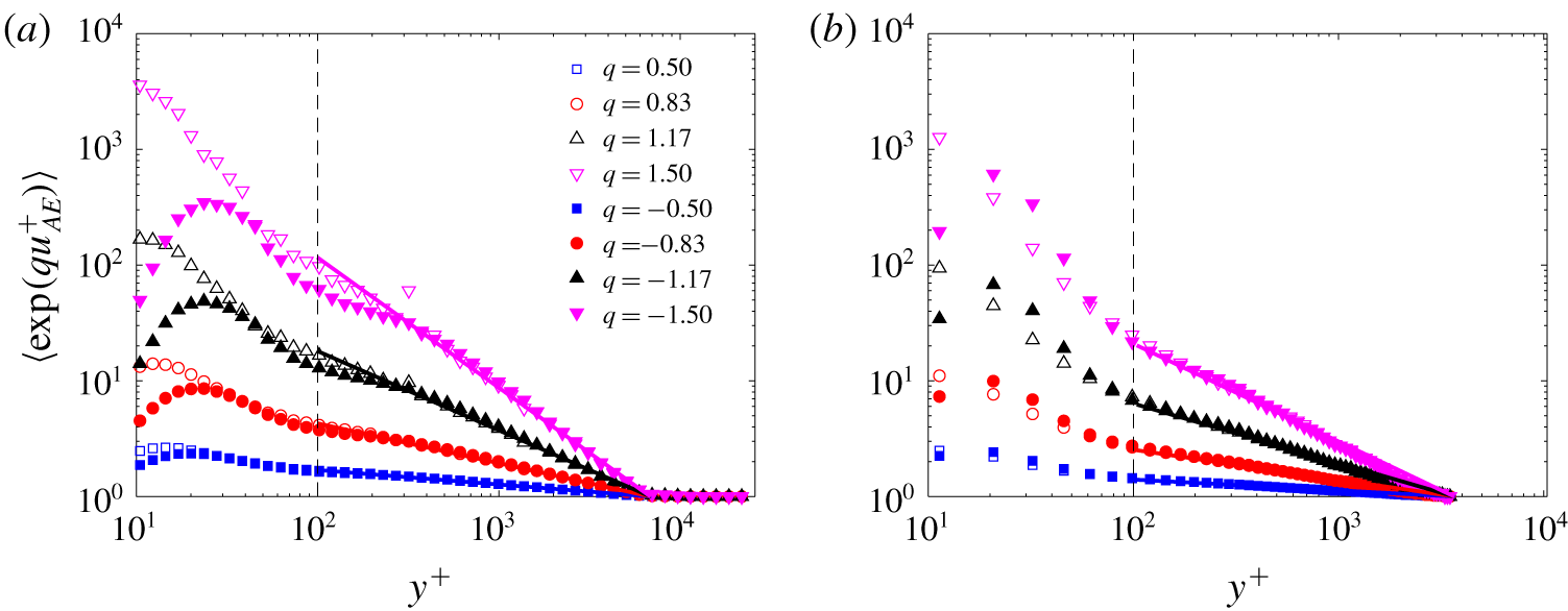
Figure 8 shows the MGFs of the attached eddies in ZPGTBL flow at  $Re_{\unicode[STIX]{x1D70F}}=13\,000$ and turbulent channel flow at
 $Re_{\unicode[STIX]{x1D70F}}=5200$ for
 $q=-1.5$ to
 $1.5$. Power-law scalings are found. The MGFs with
 $\pm q$ collapse in the logarithmic layer (
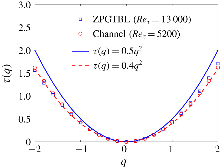
 $y^{+}>100$) and the predicted symmetry in (3.7) is borne out. In figure 9, we compare the measured
 $\unicode[STIX]{x1D70F}(q)$ to (3.8). The data are Gaussian.
Streamwise MGFs of streamwise velocity by the attached eddies in (a) turbulent boundary layer flow at  $Re_{\unicode[STIX]{x1D70F}}=13\,000$ and (b) turbulent channel flow at
 $Re_{\unicode[STIX]{x1D70F}}=5200$. The solid lines correspond to (3.7) and are not fits to the data.

The power-law exponent  $\unicode[STIX]{x1D70F}(q)$ of the MGF in ZPGTBL flow at
 $Re_{\unicode[STIX]{x1D70F}}=13\,000$ and channel flow at
 $Re_{\unicode[STIX]{x1D70F}}=5200$. The solid lines correspond to (3.8).

3.4 Two-point correlation and structure function
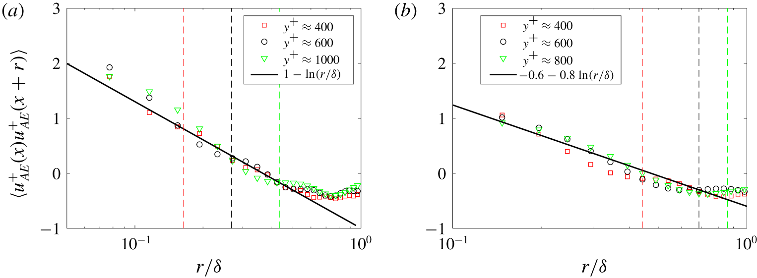
Last, we examine two-point statistics. According to the AEH, the two-point velocity correlation scales as (Yang et al. Reference Yang, Marusic and Meneveau2016a)
 $$\begin{eqnarray}\langle u^{+}(x)u^{+}(x+r)\rangle =B_{1}^{\prime }-C_{1}\ln (\unicode[STIX]{x1D6FF}/r),\end{eqnarray}$$
where  $B_{1}^{\prime }$ is a constant and
 $C_{1}$ is the same constant in (3.2a.b). If the AEH is valid, the above scaling is valid for
 $r\lesssim y/\tan \unicode[STIX]{x1D719}$. Figure 10 shows the streamwise velocity correlation due to the attached eddies in ZPGTBL flow at
 $Re_{\unicode[STIX]{x1D70F}}=13\,000$ and turbulent channel flow at
 $Re_{\unicode[STIX]{x1D70F}}=5200$. The logarithmic scaling in (3.9) is found with the predicted slope in the expected two-point displacement range.
The streamwise correlation functions of streamwise velocity by the attached eddies in (a) ZPGTBL flow at  $Re_{\unicode[STIX]{x1D70F}}=13\,000$ and (b) turbulent channel flow at
 $Re_{\unicode[STIX]{x1D70F}}=5200$. The dashed lines correspond to the upper limits (
 $r_{max}=y/\tan \unicode[STIX]{x1D719}$) of the logarithmic scaling of the two-point correlation function at different heights.

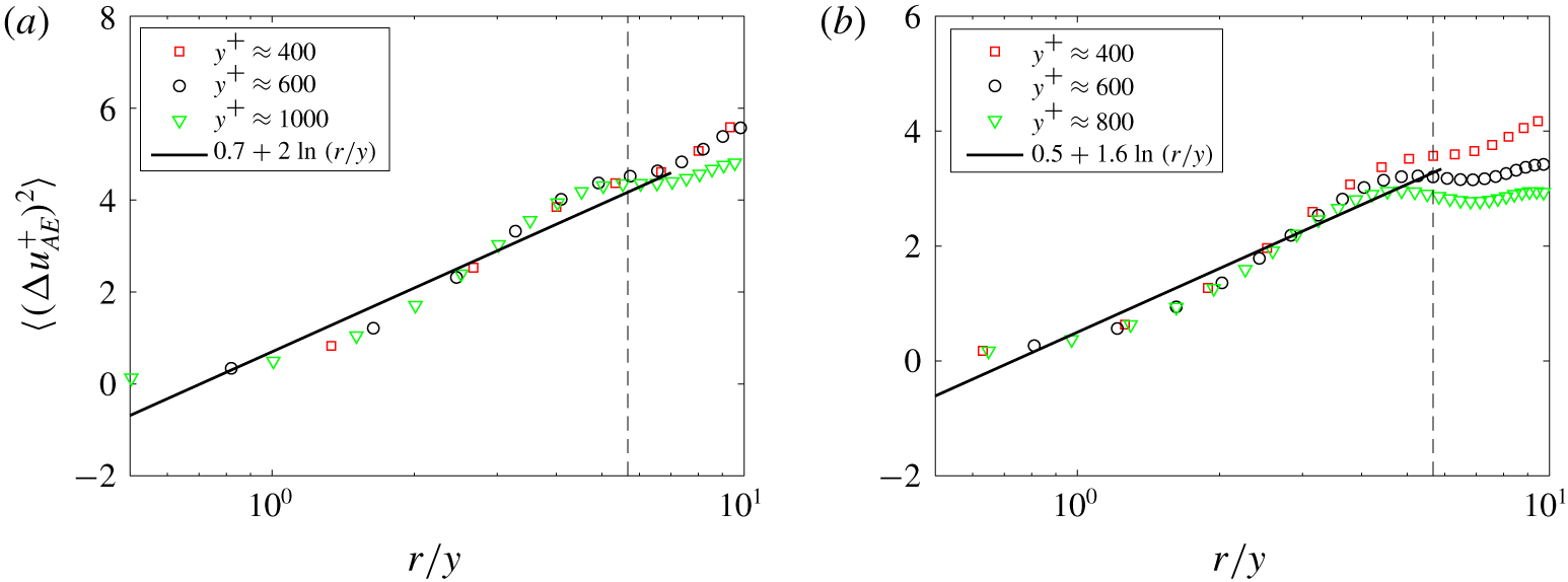
The same exercise could be done for the structure function, which scales as (Davidson et al. Reference Davidson, Nickels and Krogstad2006; Chung et al. Reference Chung, Marusic, Monty, Vallikivi and Smits2015; De Silva et al. Reference De Silva, Marusic, Woodcock and Meneveau2015; Yang et al. Reference Yang, Baidya, Johnson, Marusic and Meneveau2017)
 $$\begin{eqnarray}\langle (\unicode[STIX]{x0394}u^{+})^{2}\rangle =2C_{1}\ln (r/y)+E_{1},\end{eqnarray}$$
where  $E_{1}$ is a constant. Figure 11 shows the structure function in both ZPGTBL and channel flows. Equation (3.10) provides a good working approximation of the statistics in the expected range of two-point displacement.
The streamwise structure functions of the attached eddies in (a) ZPGTBL flow at  $Re_{\unicode[STIX]{x1D70F}}=13\,000$ and (b) turbulent channel flow at
 $Re_{\unicode[STIX]{x1D70F}}=5200$. The dashed line corresponds to the upper limit (
 $r_{max}/y=1/\tan \unicode[STIX]{x1D719}$) of the logarithmic scaling of the two-point structure function at different heights.

3.5 Summary of wall-attached eddies
In summary, we have extracted attached eddies according to the AEH, and the various statistical properties (one-point moments and MGFs, two-point correlation and structure function) of the extracted attached eddies are compared to the predictions of the AEH. Fairly good agreements are found in terms of the scaling, the constants in the scaling and the wall-normal extents of the scalings. Most notably, the extracted part of the flow is Gaussian. Hence, we may conclude that the extracted part of the flow is truly due to wall-attached eddies as described in the AEH, i.e. the eddies are wall-attached, self-similar and Gaussian.
4 Wall-detached eddies
In the previous section, we showed that the AEH is a good model for the extracted part of the flow (according to (2.1) and (2.2)). In this section, we turn our attention to the part of the flow that cannot be modelled by the AEH. Unlike the attached eddies, whose statistical behaviours are well described by the AEH, the detached eddies lack a good phenomenological model. Here, we start by examining the statistical properties of the detached eddies and see if we can get a few insights into their organization.
4.1 Streamwise velocity variance
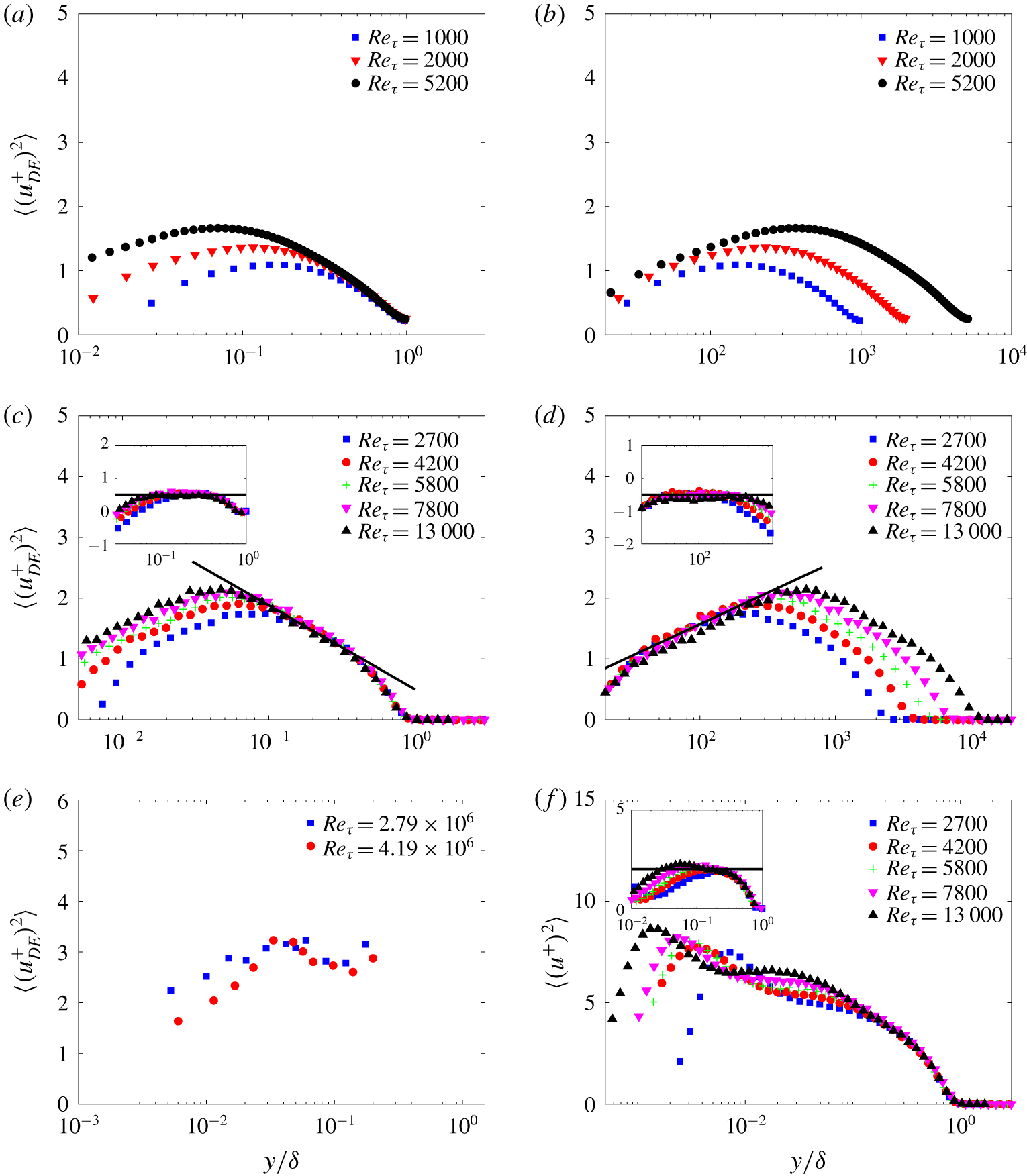
Figure 12 shows the streamwise velocity variances of detached eddies in turbulent channel flow, ZPGTBL flow and ASL flow. Unlike  $\langle (u_{AE}^{+})^{2}\rangle$, which peaks at the wall (
 $y^{+}\sim O(10^{2})$), the streamwise turbulence intensity of the detached eddies
 $\langle (u_{DE}^{+})^{2}\rangle$ peaks at the centre of the logarithmic layer. This suggests that the detached eddies centre at a distance away from the wall, which is why we had referred to these eddies as detached eddies.
Streamwise velocity variances of the detached eddies in turbulent channel flow (a,b), ZPGTBL flow (c,d) and ASL flow (e). (f) The total streamwise velocity variances in ZPGTBL flows. The insets in (c) and (d) plot  $\langle (u_{DE}^{+})^{2}\rangle +0.6\log (\,y/\unicode[STIX]{x1D6FF})$ and
 $\langle (u_{DE}^{+})^{2}\rangle -0.45\log (\,y^{+})$ as a function of
 $y/\unicode[STIX]{x1D6FF}$ and
 $y^{+}$, respectively. The inset in (f) plots
 $\langle (u^{+})^{2}\rangle +1.25\log (\,y/\unicode[STIX]{x1D6FF})$.

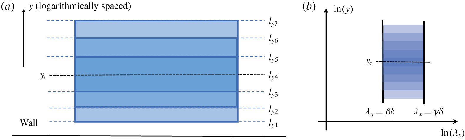
Sketches of (a) three hierarchies of wall-detached eddies;  $l_{yn}=2^{n-1}l_{y1}$. (b) The resulting pre-multiplied spectrum of the streamwise velocity fluctuations due to five hierarchies of detached eddies.

For the boundary layer data, it appears that  $\langle (u_{DE}^{+})^{2}\rangle$ follows approximately logarithmic scalings both to the left and to the right of the peak location of
 $\langle (u_{DE}^{+})^{2}\rangle$. To diagnose the two scalings, we subtract the logarithmic part of the scaling from
 $\langle (u_{DE}^{+})^{2}\rangle$. The compensated plots are shown in the insets of figure 12(c,d), and we see plateaus. We could also compare the quality of these logarithmic scalings to the well-accepted logarithmic law of the total streamwise velocity
 $\langle (u^{+})^{2}\rangle$ in the ZPGTBL flow data. Comparing figures 12(c), 12(d) and 12(f), it should be clear that the quality of the logarithmic scalings in figure 12(f) are equally good (or equally bad) as the ones in figure 12(c,d). Compared to the boundary layer data, the channel flow data are at a moderate Reynolds number and the ASL data are subjected to freestream/thermal effects. Consequently, only hints of these two logarithmic scalings could be found in channel and ASL data.
If we follow Townsend, the two logarithmic scalings in  $\langle u_{DE}^{2}\rangle$ imply that the detached eddies may be modelled as a series of eddies centred at
 $y_{c}$, as sketched in figure 13. If the detached eddies do organize as in figure 13, determining the centre location
 $y_{c}$ is probably the most important. In the absence of viscous effects, the centre location
 $y_{c}$ corresponds to the peak location of
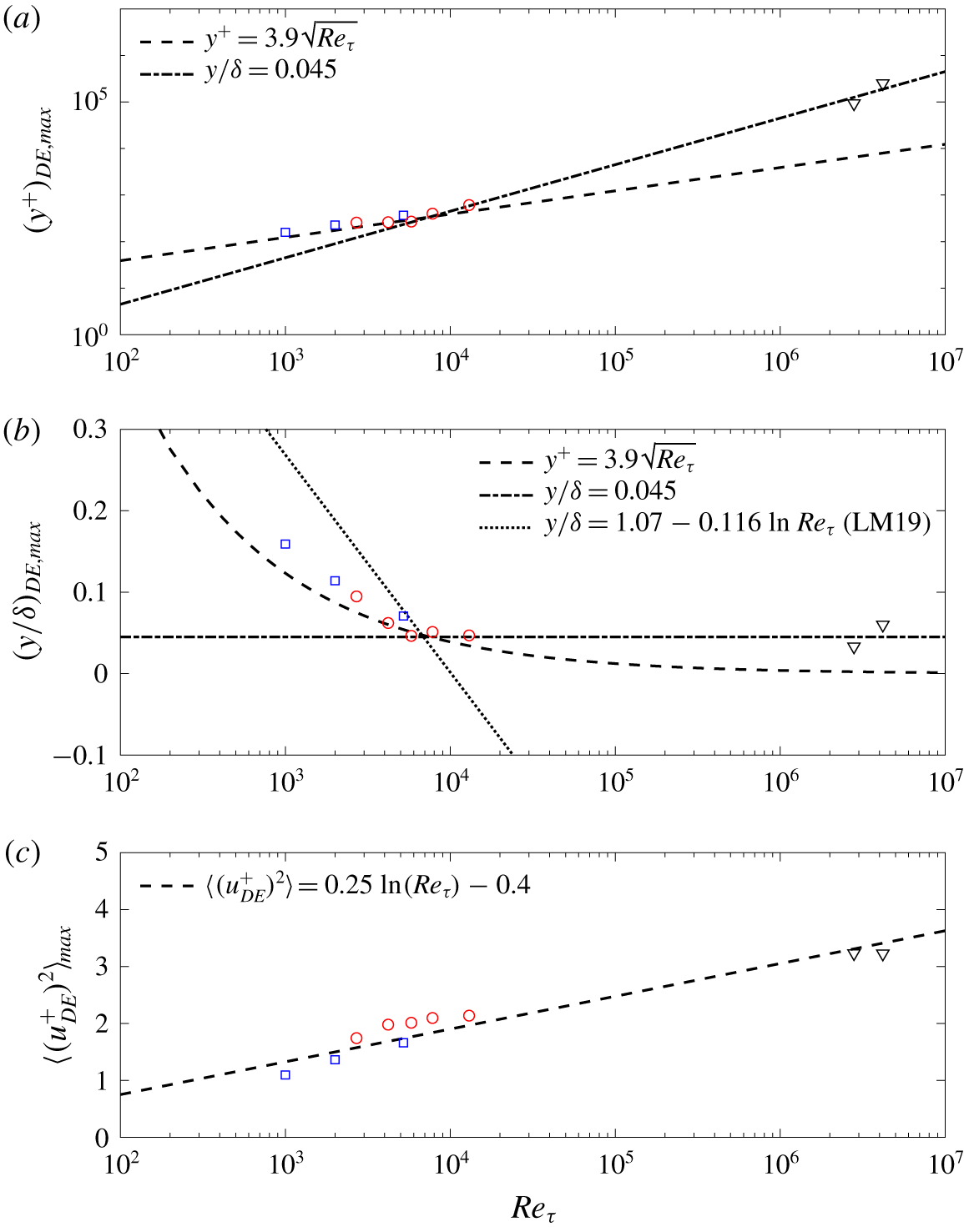
 $\langle (u_{DE}^{+})^{2}\rangle$. Figure 14 shows the wall-normal positions and the magnitudes of
 $\max [\langle (u_{DE}^{+})^{2}\rangle ]$. The Reynolds number dependence of
 $y_{DE,max}$ is unclear from the available data. The results of turbulent channel and ZPGTBL flows seem to suggest that
 $y_{DE,max}^{+}=3.9\sqrt{Re_{\unicode[STIX]{x1D70F}}}$ between
 $Re_{\unicode[STIX]{x1D70F}}\sim O(10^{3})$ and
 $O(10^{4})$, but the ASL data seem to suggest that
 $(\,y/\unicode[STIX]{x1D6FF})_{DE,max}\rightarrow 0.045$. Last, from figure 14(c), we see that the peak value
 $\langle (u_{DE}^{+})^{2}\rangle _{max}$ follows a logarithmic scaling with respect to the Reynolds number, which is consistent with previous studies (Pullin, Inoue & Saito Reference Pullin, Inoue and Saito2013; Vincenti et al. Reference Vincenti, Klewicki, Morrill-Winter, White and Wosnik2013; Vallikivi, Hultmark & Smits Reference Vallikivi, Hultmark and Smits2015).
The wall-normal locations (a,b) and the magnitudes (c) of the maximum streamwise turbulence intensity due to the detached eddies as a function of the Reynolds number. The squares are turbulent channel flow data. The red circles are boundary layer data. The black triangles are ASL data. The Reynolds number variance of the peak location  $y/\unicode[STIX]{x1D6FF}$ with
 $\unicode[STIX]{x1D706}^{+}>1000$ from Lee & Moser (Reference Lee and Moser2019) is indicated by LM19 in (b).

In Lee & Moser (Reference Lee and Moser2019), the authors defined the large scales as  $\unicode[STIX]{x1D706}^{+}>1000$. The streamwise velocity variance due to such defined large scales has a peak. The peak value
 $\langle (u^{+})^{2}\rangle _{LS}$ increases and the peak location
 $y/\unicode[STIX]{x1D6FF}$ decreases as a function of the Reynolds number. In figure 14(b), the location is shown for comparison. The difference is probably expected considering the difference in our definitions.
4.2 High-even-order moments and MGFs
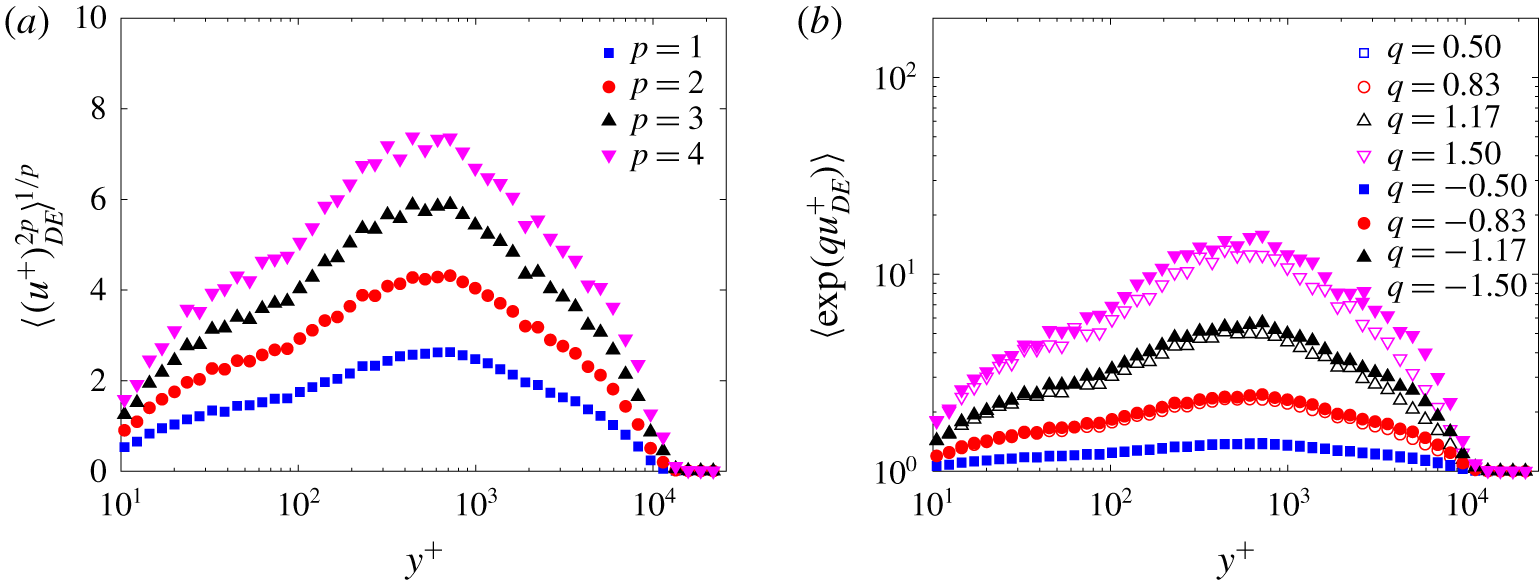
If the organization of the detached eddies is as sketched in figure 13, following the same argument that leads to the logarithmic scaling of the even-order moments, we expect logarithmic scaling of the even-order moments for the detached eddies to the left and to the right of  $y_{c}$. Figure 15 shows the even-order moments and MGFs of the detached eddies. Hints of possible logarithmic scalings as a function of the wall-normal distance are found in Figure 15(a) to the left and to the right of
 $y_{c}$, as well as hints of possible power-law scalings of the MGFs, but because of the limited extents of the scale ranges to the left and to the right of
 $y_{c,DE}$, neither of the two scalings is very conclusive.
Even-order moments (a) and MGFs (b) of streamwise velocity by the detached eddies in turbulent boundary layer flows at  $Re_{\unicode[STIX]{x1D70F}}=13\,000$.

5 Inter-scale interactions
Having looked at the statistical properties of the attached eddies and the detached eddies separately, in this section we study the interactions between the small-scale eddies, the attached eddies and the detached eddies. Here, we focus on the particular inter-scale interaction of amplitude modulation, where the (loosely defined) small-scale eddies are modulated by the (loosely defined) large-scale eddies. This form of inter-scale interaction has received considerable attention in the recent literature (Hutchins & Marusic Reference Hutchins and Marusic2007; Mathis et al. Reference Mathis, Hutchins and Marusic2009; Chung & McKeon Reference Chung and McKeon2010; Guala, Metzger & McKeon Reference Guala, Metzger and McKeon2011; Ganapathisubramani et al. Reference Ganapathisubramani, Hutchins, Monty, Chung and Marusic2012; Agostini & Leschziner Reference Agostini and Leschziner2014; Anderson Reference Anderson2016; Dogan, Hanson & Ganapathisubramani Reference Dogan, Hanson and Ganapathisubramani2016; Pathikonda & Christensen Reference Pathikonda and Christensen2017, Reference Pathikonda and Christensen2019; Howland & Yang Reference Howland and Yang2018; Liu, Wang & Zheng Reference Liu, Wang and Zheng2019).
In anticipation of the results, we briefly review one of the previously used quantifications of amplitude modulation in Mathis et al. (Reference Mathis, Hutchins and Marusic2009):
 $$\begin{eqnarray}R=\frac{\langle u_{L}^{+}E_{L}(u_{S}^{+})\rangle }{\text{STD}(u_{L}^{+})\text{STD}(E_{L}(u_{S}^{+}))},\end{eqnarray}$$
where  $u_{S}$ and
 $u_{L}$ are the (loosely defined) small- and large-scale components of the streamwise velocity,
 $E(\cdot )$ is the envelope of the bracketed signal and STD
 $(\cdot )$ is the standard deviation of the bracketed quantity. Thus-defined
 $R$ behaves similarly to the skewness factor
 $S=\langle (u^{+})^{3}\rangle /\langle (u^{+})^{2}\rangle ^{3/2}$ (Schlatter & Örlü Reference Schlatter and Örlü2010). Mathis et al. (Reference Mathis, Marusic, Hutchins and Sreenivasan2011) compared
 $R$ and
 $S$ and showed that the behaviour of
 $\langle 3u_{L}^{+}u_{S}^{+2}\rangle /\langle (u^{+})^{2}\rangle ^{3/2}$ is similar to that of
 $R$, which may serve as an alternative measure of amplitude modulation. Recently, Duvvuri & McKeon (Reference Duvvuri and McKeon2015) showed that
 $\langle 3u_{L}^{+}u_{S}^{+2}\rangle /\langle (u^{+})^{2}\rangle ^{3/2}$ is proportional to
 $R$ for any statistically stationary signal. Following the previous literature, in the following, we will use the scale-decomposed skewness to quantify amplitude modulation.
In this work, we have decomposed the streamwise velocity fluctuation into SE (small-scale eddies), AE (attached eddies) and DE (detached eddies), and therefore the skewness factor can be decomposed triadically, i.e.
 $$\begin{eqnarray}\displaystyle \langle (u^{+})^{3}\rangle & = & \displaystyle \langle (u_{SE}^{+}+u_{AE}^{+}+u_{DE}^{+})^{3}\rangle \nonumber\\ \displaystyle & = & \displaystyle \langle (u_{SE}^{+})^{3}\rangle +\langle (u_{AE}^{+})^{3}\rangle +\langle (u_{DE}^{+})^{3}\rangle +3\langle (u_{SE}^{+})^{2}u_{AE}^{+}\rangle +3\langle (u_{AE}^{+})^{2}u_{SE}^{+}\rangle \nonumber\\ \displaystyle & & \displaystyle +\,3\langle (u_{SE}^{+})^{2}u_{DE}^{+}\rangle +3\langle (u_{DE}^{+})^{2}u_{SE}^{+}\rangle \nonumber\\ \displaystyle & & \displaystyle +\,3\langle (u_{AE}^{+})^{2}u_{DE}^{+}\rangle +3\langle (u_{DE}^{+})^{2}u_{AE}^{+}\rangle \nonumber\\ \displaystyle & & \displaystyle +\,6\langle u_{SE}^{+}u_{AE}^{+}u_{DE}^{+}\rangle .\end{eqnarray}$$
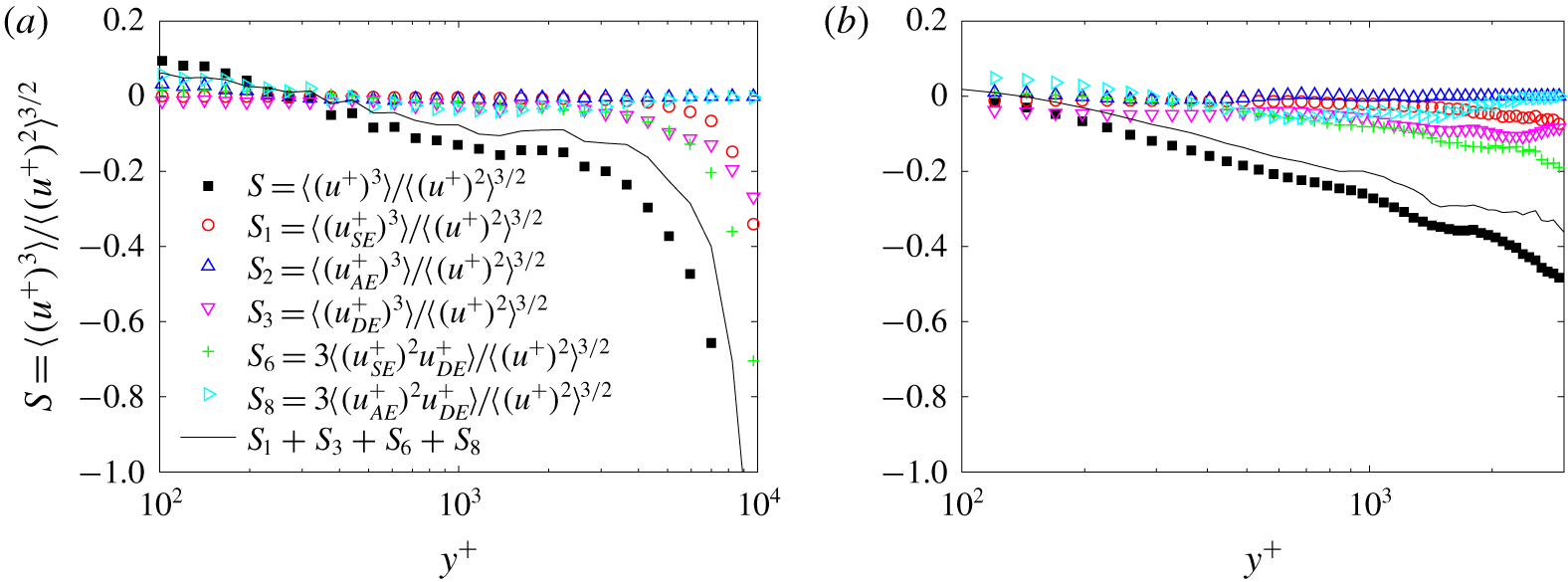
In figure 16, we show the wall-normal dependence of a few dominant components in (5.2) in the ZPGTBL flow at  $Re_{\unicode[STIX]{x1D70F}}=13\,000$ and the channel flow at
 $Re_{\unicode[STIX]{x1D70F}}=5200$. The skewness of the attached eddies, i.e.
 $S_{2}$ in figure 16, is very close to zero in both the ZPGTBL and channel flows. This is consistent with the assumed Gaussian behaviour of the attached-eddy-induced velocities in the AEH. The most significant contributions to
 $S$ come from the detached eddies, the small-scale eddies and their interactions. The interaction between the attached eddies and the detached eddies, i.e.
 $3\langle (u_{SE}^{+})^{2}u_{AE}^{+}\rangle$, is very close to zero and is not shown in figure 16. The results suggest that, at a given wall-normal location, the main inter-scale interaction is among the detached eddies and the small-scale eddies. A recent study using the QLOA dataset also reported a similar one-point multi-scale amplitude-modulation phenomenon (Liu et al. Reference Liu, Wang and Zheng2019).
Skewness of the streamwise velocity in (a) ZPGTBL flow at  $Re_{\unicode[STIX]{x1D70F}}=13\,000$ and (b) turbulent channel flow at
 $Re_{\unicode[STIX]{x1D70F}}=5200$. ▪,
 $S=\langle (u^{+})^{3}\rangle /\langle (u^{+})^{2}\rangle ^{3/2}$; ○,
 $S_{1}=\langle (u_{SE}^{+})^{3}\rangle /\langle (u^{+})^{2}\rangle ^{3/2}$; ▵,
 $S_{2}=\langle (u_{AE}^{+})^{3}\rangle /\langle (u^{+})^{2}\rangle ^{3/2}$; ▿,
 $S_{3}=\langle (u_{DE}^{+})^{3}\rangle /\langle (u^{+})^{2}\rangle ^{3/2}$;
 $+$,
 $S_{6}=3\langle (u_{SE}^{+})^{2}u_{DE}^{+}\rangle /\langle (u^{+})^{2}\rangle ^{3/2}$; ▹,
 $S_{8}=3\langle (u_{AE}^{+})^{2}u_{DE}^{+}\rangle /\langle (u^{+})^{2}\rangle ^{3/2}$; black solid line,
 $S_{1}+S_{3}+S_{6}+S_{8}$.

The above analysis is one-point analysis. Next, we study the modulation of the near-wall turbulence by the attached eddies and the detached eddies. To do that, we use the two-point synchronous measurements in ZPGTBL flow at  $Re_{\unicode[STIX]{x1D70F}}=15\,000$ (Baars et al. Reference Baars, Talluru, Hutchins and Marusic2015) and turbulent channel flow data at
 $Re_{\unicode[STIX]{x1D70F}}=5200$ (one snapshot). We measure the amplitude modulation of the near-wall turbulence by the outer flow using the following correlation coefficient defined in Bernardini & Pirozzoli (Reference Bernardini and Pirozzoli2011):
 $$\begin{eqnarray}C_{AM}(\,y_{1},y_{2})=\langle u_{L}(\,y_{1})E_{L}(u_{S}(\,y_{2}))\rangle\end{eqnarray}$$
in which  $y_{1}$ and
 $y_{2}$ are the wall-normal locations of the traversing and fixed probes, respectively (
 $y_{2}^{+}=4.33$ is fixed),
 $u_{L}$ may be the attached eddies, the detached eddies or the large-scale modes with
 $\unicode[STIX]{x1D706}_{x}^{+}>7000$ and
 $u_{S}(\,y_{2})$ is the near-wall small-scale signal with
 $\unicode[STIX]{x1D706}_{x}^{+}<7000$, following Mathis, Hutchins & Marusic (Reference Mathis, Hutchins and Marusic2011). We apply a time shift at
 $y_{1}$ in (5.3) to account for the inclination of the turbulent eddies. Note that, because the attached eddies are not formally defined at a wall-normal distance smaller than the viscous cutoff, i.e.
 $y^{+}=100$, the near-wall small-scale turbulence, defined as
 $\unicode[STIX]{x1D706}_{x}^{+}<7000$, does not formally overlap with the attached eddies.
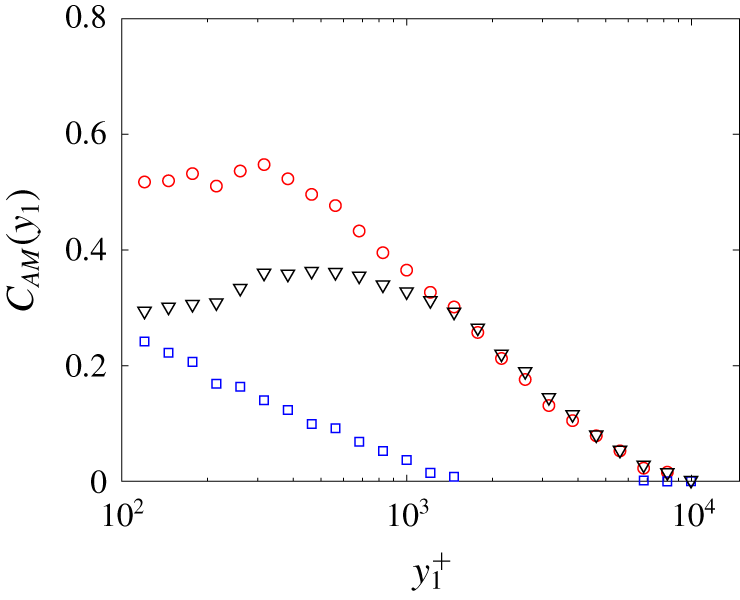
Two-point amplitude-modulation coefficient  $C_{AM}(\,y_{1})$ in ZPGTBL flow at
 $Re_{\unicode[STIX]{x1D70F}}=15\,000$, where
 $u_{L}$ is the the large-scale modes of
 $\unicode[STIX]{x1D706}_{x}^{+}>7000$ (○), the attached eddies (▫) or the detached eddies (▿).

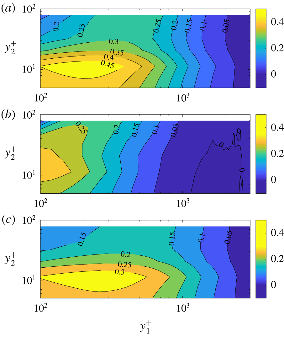
Two-point amplitude-modulation coefficient map  $C_{AM}(\,y_{1},y_{2})$ in turbulent channel flow at
 $Re_{\unicode[STIX]{x1D70F}}=5200$ computed with the velocity signals from the (a) large-scale modes (
 $\unicode[STIX]{x1D706}_{x}^{+}>7000$), (b) attached eddies and (c) detached eddies.

Figure 17 shows the wall-normal variations of  $C_{AM}(\,y_{1})$ with different
 $u_{L}(\,y_{1})$ in ZPGTBL flow. We see that the coefficient calculated with the large-scale modes of
 $\unicode[STIX]{x1D706}_{x}^{+}>7000$ has a peak at
 $y^{+}=300$–
 $400$. The coefficients calculated with the attached or detached eddies are reminiscent of their one-point intensities: the amplitude modulation by the detached eddies has its peak at the centre of the logarithmic region, while that by the attached eddies decreases log-linearly with the wall-normal height. Similar results are obtained in turbulent channel flow at
 $Re_{\unicode[STIX]{x1D70F}}=5200$, which are presented in a two-dimensional
 $C_{AM}(\,y_{1},y_{2})$ map in figure 18. The present results suggest that both the attached and detached eddies contribute to the amplitude modulation of the near-wall small-scale motions. Nonetheless, their contributions are quantitatively different.
6 Instantaneous features of the decomposed eddies
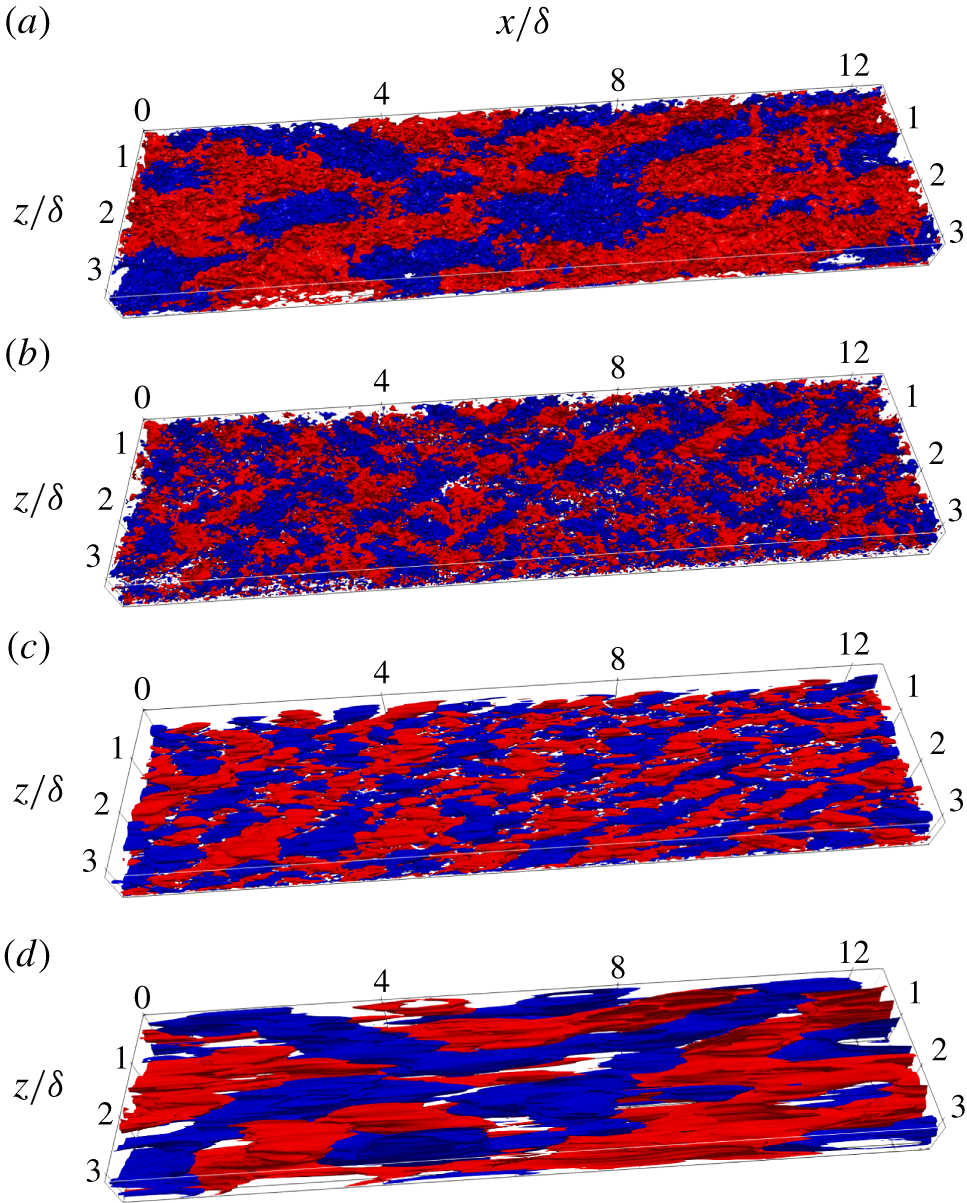
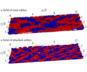
Instantaneous  $|u^{+}|=1$ isosurfaces (red for positive and blue for negative values) from the (a) total eddies, (b) small-scale eddies, (c) attached eddies and (d) detached eddies.

Townsend only defined attached eddies in a statistical sense, without attaching any specific geometry to the attached eddies, nor relating any instantaneous flow features to the attached eddies. So far, we have followed Townsend and have focused on the statistical behaviour of the decomposed eddies. Nonetheless, taking a look at the instantaneous velocity fields that correspond to the decomposed eddies would still be instructive. Figure 19 shows the  $|u^{+}|=1$ isosurfaces of the total velocity, the small-scale eddies, the attached eddies and the detached eddies in channel flow at
 $Re_{\unicode[STIX]{x1D70F}}=5200$. For better presentation, the figure shows the instantaneous velocities in a truncated domain of
 $0\leqslant x\leqslant 4\unicode[STIX]{x03C0}$,
 $100\leqslant y^{+}$,
 $y\leqslant \unicode[STIX]{x1D6FF}_{i}$ and
 $0\leqslant z\leqslant \unicode[STIX]{x03C0}$. We see alternating high- and low-speed regions in every component. Meandering streaks are found in the velocity field due to detached eddies. Both the attached eddies and the small scales show coherence in oblique orientations with respect to the streamwise direction. Considering that attached eddies (and detached eddies) are only defined from a statistical standpoint, we will refrain from discussing details of the instantaneous flow fields.
7 Conclusions
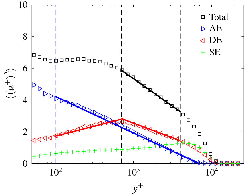
According to Townsend, the attached eddies in the AEH are defined only in a statistical sense, being responsible for part of the scales in the flow field. Following Townsend (Reference Townsend1976), we proposed a scale decomposition scheme and extracted the part of the flow that is due to attached eddies from boundary layer, channel and atmospheric boundary layer flows. By comparing the statistical properties of the extracted eddies to those promised by the AEH, we showed that the AEH is a good model for the extracted part of the flow, and notably that part of the flow is Gaussian. Hence, the reason that the AEH does not capture some of the statistical behaviours of the flow in the logarithmic layer is because there are other energy-containing eddies than the attached eddies, which are the small (Kolmogorov)-scale eddies and the large-scale detached eddies. Unlike the attached eddies whose statistical behaviours are well captured by the AEH, the detached eddies lack a well-validated phenomenological model. In this work, we studied the statistical properties of the detached eddies. Although not conclusive, the statistical behaviour of the detached eddies suggests that these eddies can be modelled as flow structures centred at the midpoint of the logarithmic layer. Finally, we studied the interaction among the small-scale eddies, the attached eddies and the detached eddies. We focused on the particular inter-scale interaction of amplitude modulation. We found first that at a given wall-normal height, the main inter-scale interaction is between the small-scale eddies and the detached eddies, and second that both the attached and detached eddies contribute to the amplitude modulation of the near-wall small-scale motions. Putting together the AEH and our phenomenological model for the detached eddies, we can phenomenologically explain the appearance of the streamwise turbulence kinetic energy plateau in the mesolayer, i.e.  $100<y^{+}<700$, in ZPGTBL flow at
 $Re_{\unicode[STIX]{x1D70F}}=13\,000$ as shown in figure 20. In this region, the streamwise turbulence kinetic energy of the attached eddies decreases as a function of
 $y$ but that of the detached eddies increases as a function of
 $y$. The overall effect is the plateau in the total streamwise turbulence kinetic energy. Last, an interesting but unexplored question is whether we could apply a spanwise filter to extract wall-attached eddies. One difficulty in so doing is the determination of the spanwise extent of wall-attached eddies. While Jiménez & Hoyas (Reference Jiménez and Hoyas2008), Hwang (Reference Hwang2015), Hellström et al. (Reference Hellström, Marusic and Smits2016) and Hwang & Sung (Reference Hwang and Sung2018) looked at the spanwise scale of attached eddies, compared to the streamwise extent, the spanwise extent of the attached eddies is still less well established.
Streamwise velocity variance with decomposition of specific contributions by the attached eddies (AE), the detached eddies (DE) and the small-scale eddies (SE).

Acknowledgements
We express our sincere gratitude to I. Marusic, N. Hutchins, W. J. Baars and R. Baidya for providing the Melbourne wind-tunnel measurement data, G.-H. Wang and H.-H. Gu for providing the QLOA data, M. Lee and R. Moser for making the channel flow database publicly available, Z. Wu for aiding in the access of the channel flow data in the Johns Hopkins Turbulence Database, as well as C. Meneveau and D. Gayme for helpful suggestions. The authors also appreciate the valuable comments made by the anonymous referees which help to improve both the quality and the presentation of this paper. Financial support by grants from the National Natural Science Foundation of China (11490553, 11972175) is gratefully acknowledged. R.H. is grateful for the hospitality of the Department of Mechanical Engineering of the Johns Hopkins University and the financial support of the China Scholarship Council for his visit.
Declaration of interests
The authors report no conflict of interest.
Appendix A. The effect of filter
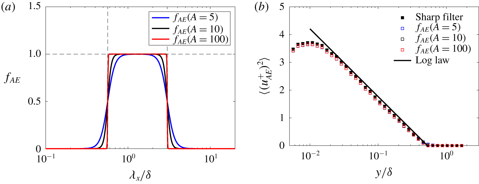
Considering (2.1) and (2.2), a sharp cutoff filter is used to extract the part of the flow that is due to wall-attached eddies. In this appendix, we show that the type of filter does not affect much, if at all, our results. Here, we use a continuous spectral filter comparing the results with those from using a sharp filter. The continuous spectral filter is defined based on a hyperbolic tangent function as
 $$\begin{eqnarray}f_{AE}(\unicode[STIX]{x1D706}_{x},y;A)=H(\unicode[STIX]{x1D706}_{x},y;A)\cdot G(\unicode[STIX]{x1D706};A),\end{eqnarray}$$
in which  $H(\unicode[STIX]{x1D706}_{x},y;A)$ and
 $G(\unicode[STIX]{x1D706},\unicode[STIX]{x1D6FF};A)$ correspond to the small-scale and large-scale cutoffs in (2.1), where
 $$\begin{eqnarray}\displaystyle & \displaystyle H(\unicode[STIX]{x1D706}_{x},y;A)=\frac{1+\tanh \left[A\cdot \ln (\unicode[STIX]{x1D706}_{x}/(\unicode[STIX]{x1D6FC}y))\right]}{2}, & \displaystyle\end{eqnarray}$$
 $$\begin{eqnarray}\displaystyle & \displaystyle G(\unicode[STIX]{x1D706},\unicode[STIX]{x1D6FF};A)=\frac{1+\tanh \left[A\cdot \ln (\unicode[STIX]{x1D706}_{x}/(\unicode[STIX]{x1D6FD}\unicode[STIX]{x1D6FF}))\right]}{2} & \displaystyle\end{eqnarray}$$
and  $A$ is the parameter controlling the sharpness of the filter. In the logarithmic layer, the local wall-normal coordinate provides a local length scale (and in the absence of the viscous effects, that is the only length scale). Hence, the sharpness scales with
 $y$ at the small-scale cutoff and
 $\unicode[STIX]{x1D6FF}$ at the large-scale cutoff.
The effect filter on the statistics of attached eddies. (a) Continuous filters with different values of  $A$. The wall-normal location is
 $y/\unicode[STIX]{x1D6FF}=0.1$. (b) The streamwise velocity variances obtained with different filters in (a). The solid line corresponds to the logarithmic law (3.2a.b).

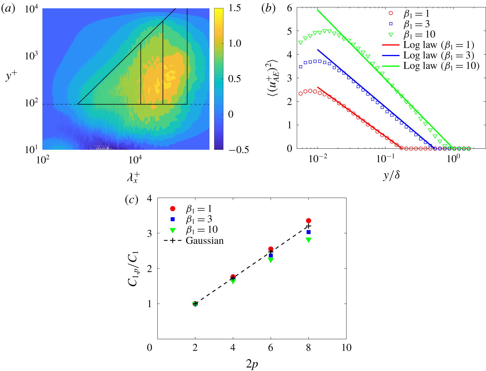
The effect of large-scale cutoff on the extracted statistics due to attached eddies. (a) The region due to attached eddies with different large-scale cutoff ( $\unicode[STIX]{x1D6FD}_{1}=1,3,10$). (b) The streamwise velocity variances due to attached eddies with different large-scale cutoffs as well as the predictions from the AEH, i.e. (3.2a.b). (c) The coefficient ratios
 $C_{1,p}/C_{1}$ of high-even-order moments as a function of moment order
 $2p$ for different large-scale cutoffs.

Figure 21(a) shows the filters with various  $A$ values. The sharpness at the small- and large-scale cutoffs increases as
 $A$ increases. The filter with
 $A=5$ is rather smooth, whereas that with
 $A=100$ is very close to the sharp cutoff filter in (2.1) and (2.2). We apply the continuous filter with various
 $A$ values to the ZPGTBL flow data at
 $Re_{\unicode[STIX]{x1D70F}}=13\,000$, and the resulting streamwise velocity variances of the attached eddies are shown in figure 21(b). The results are essentially the same, indicating that the sharpness of the filter will probably not affect our conclusions.
Appendix B. The effect of large-scale cutoff wavelength
In § 2.2, we argued that using a more conservative cutoff, the extracted part of the flow will still be fully described by the AEH. Here, we show that this statement is true. In addition, we show that an aggressive cutoff will include scales that do not belong to attached eddies and have a negative impact on the results. We choose two different large-scale cutoffs, namely  $\unicode[STIX]{x1D706}_{x}=\unicode[STIX]{x1D6FF}$ (
 $\unicode[STIX]{x1D6FD}_{1}=1$) and
 $\unicode[STIX]{x1D706}_{x}=10\unicode[STIX]{x1D6FF}$ (
 $\unicode[STIX]{x1D6FD}_{1}=10$). In the main text,
 $\unicode[STIX]{x1D706}_{x}=3\unicode[STIX]{x1D6FF}$ (
 $\unicode[STIX]{x1D6FD}_{1}=3$) for ZPGTBL flow. Figure 22(a) shows the enclosed regions. The region is a trapezium for
 $\unicode[STIX]{x1D6FD}_{1}=10$ because it cuts off at
 $y=\unicode[STIX]{x1D6FF}$. As per our discussion in § 2.2, being conservative and using
 $\unicode[STIX]{x1D6FD}_{1}=1$, the extracted part of the flow will still be well modelled by the AEH; however, being very aggressive and using
 $\unicode[STIX]{x1D6FD}_{1}=10$, the statistical properties of the extracted part of the flow would not be captured by the AEH.
The streamwise velocity variances with different  $\unicode[STIX]{x1D6FD}_{1}$ are shown in figure 22(b). The corresponding predictions from the AEH are given by solid lines, i.e. (3.2a.b). The large-scale cutoff shows up in
 $\unicode[STIX]{x1D6FF}_{i}$ hence the end location of the logarithmic scaling. The coefficient
 $C_{1}$ in (3.2a.b) increases as a function of the large-scale cutoff, the values of which are around 0.9, 1.0 and 1.3 for
 $\unicode[STIX]{x1D6FD}_{1}=1$,
 $3$ and
 $10$, respectively. The results for
 $\unicode[STIX]{x1D6FD}_{1}=1$ and
 $3$ agree well with the AEH, whereas the result for
 $\unicode[STIX]{x1D6FD}_{1}=10$ deviates from the expected logarithmic scaling. Figure 22(c) shows the measured
 $C_{1,p}/C_{1}$ for high-even-order moments. The use of
 $\unicode[STIX]{x1D6FD}_{1}=1$ or
 $\unicode[STIX]{x1D6FD}_{1}=3\unicode[STIX]{x1D6FF}$ leads to Gaussian behaviour, which agrees well with the AEH, but
 $\unicode[STIX]{x1D6FD}_{1}=10$ results in sub-Gaussian behaviour, similar to the total velocity (Meneveau & Marusic Reference Meneveau and Marusic2013).