1. INTRODUCTION
Nonlinear filtering and estimation based on Bayesian theory has attracted intensive investigation. However, the optimal Bayesian filter is difficult to solve for state estimation; therefore, it is usually reduced to the problem of how to compute multi-dimensional Gaussian-weighted integrals. The Kalman Filter (KF) is derived in this way and treated as the typical suboptimal method in the Bayesian framework, which is accomplished by assuming that the predictive density of the joint state-measurement vector is Gaussian distributed. Typical filters in the Kalman filter framework are the Extended Kalman Filter (EKF) (Kalman and Bucy, Reference Kalman and Bucy1961; Gelb, Reference Gelb1974), the Unscented Kalman Filter (UKF) (Julier and Uhlmann, Reference Julier and Uhlmann2000; Julier, Reference Julier2002), Centre Difference Kalman Filter (CDKF) (Norgaard et al., Reference Norgaard, Poulsen and Ravn2000a; Reference Norgaard, Poulsen and Ravn2000b), Gauss-Hermite Quadrature Filter (GHQF) (Ito and Xiong, Reference Ito and Xiong2000) and Cubature Kalman Filter (CKF) (Lu et al., Reference Lu, Dong and Xiaoqian2018). The above extended forms of KF are collectively referred to as the Gaussian approximation filters, which have proven to be extremely useful in a wide range of applications, including: noise reduction of signals, trajectory tracking and in the control of linear and nonlinear systems. In recent years, the predictive filter and its extended forms (Lu et al., Reference Lu, Xiaoqian and Arun2015a; Reference Lu, Yu, Xiaoqian and Yong2015b; Reference Lu, Qiang, Xiaoqian and Yong2014; Lu and Hengnian, Reference Lu and Hengnian2016a) have attracted wide attention, and have some abilities to deal with model errors in order to improve filtering performance. In addition, Habibi (Reference Habibi2007) and Gadsden et al. (Reference Gadsden, Al-Shabi, Arasaratnam and Habibi2014) proposed a new type of filter referred as to the Smooth Variable Structure Filter (SVSF). This is a predictor-corrector estimator based on sliding mode concepts and a Kalman filter, and can be applied on both linear or nonlinear systems and measurements. Based on this concept, Lu et al. (Reference Lu, Yongqiang, Zhidong, Hengnian and Arun2017; Reference Lu, Junqiang, Lei and Hengnian2016; Reference Lu, Dong, Han and Wang2018) and Lu and Hengnian (Reference Lu and Hengnian2016b) proposed the Predictive Smooth Variable Structure Filter (PSVSF) based on the sliding mode strategy and predictive filter, which does not have to linearize the measurement model in order to enhance the ability to deal with nonlinear problems.
Among these Gaussian approximation filters, the CKF is proposed based on the third-degree spherical-radial cubature rule, which is shown to be more stable than the UKF by theoretical analysis. In order to obtain higher precision, the High-degree Cubature Kalman Filter (HCKF) has been proposed by Bin et al. (Reference Bin, Ming and Yang2013) with arbitrary degrees of accuracy in computing the spherical and radial integrals. The high-degree CKFs of this class can achieve accuracy and stability performances close to those of the GHQF, but the computational loads associated with them are also very high, and these increase polynomially with the state-space dimensions. Hence, it is difficult to apply these filters on board satellites for higher dimensional problems.
In recent years, Satellite Formation Flying (SFF), endowed with various advantages compared to a single satellite, has become a focus of research (Kristiansen and Nicklasson, Reference Kristiansen and Nicklasson2009; Cao and Misra, Reference Cao and Misra2015). These advantages make SFF an ideal tool to achieve various types of space mission. All SFF missions rely heavily on precise relative position and attitude information. Therefore, relative navigation technology with excellent filtering algorithms is very important for the future use of SFF. According to the existing achievements, the relative navigation of SFF is typically described by a form of Six-Degrees Of Freedom (6-DOF) relative motion model (Xing et al., Reference Xing, Cao, Zhang, Guo and Wang2010; Cao et al., Reference Cao, Chen and Misra2015) with 12 dimension state variables. The performance of relative navigation and attitude estimation is heavily dependent on the estimation methodologies. Hence, the EKF, UKF and Unscented Predictive Filter (UPF) (Tang et al., Reference Tang, Yan and Zhong2010) have been used in the past to obtain good estimation results. However, the above methods can only capture second-degree accuracy for relative navigation due to their theoretical limitations. Instead of traditional methods, the High-degree CKF (HCKF) is employed to obtain better estimation results, which is the purpose of this study. This is in spite of the fact that the calculation burden of HCKF increases polynomially with the dimension for an arbitrary degree of precision.
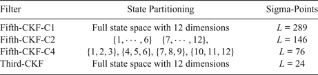
Therefore, a reduction strategy for the HCKF based on partitioning of the state-space is proposed as the main theoretical innovation of this paper, referred to as the Multiple HCKF (MHCKF). For the relative navigation problem, the HCKF needs 289 sigma points by using the equation to capture the fifth-degree estimation accuracy, which is difficult to apply on board. However, if we partition the states into two parts, the number of total sigma points are 146. Similarly, if we partition the states into four parts, the number of sigma points employed can be reduced to 76 for relative navigation estimation. Obviously, the partitioning strategy can greatly reduce the calculation burden for the high-dimensions estimation problem. However, this strategy will damage the coupling relationship between the state variables, which will reduce the estimation precision. Therefore, the sequence orthogonal principle is introduced to improve the robustness of the estimation performance, in order to decrease the effect of the partitioning strategy. To demonstrate this, several forms of MRHCKF are simulated to compare with the traditional fifth-degree CKF for relative navigation, in order to show their advantages and characteristics.
The organisation of this paper is as follows: The 6-DOF relative navigation model of SFF is derived in Section 2. The arbitrary degree-CKF is reviewed in Section 3. Then, the MHCKF is proposed by using the partitioning strategy and sequence orthogonal principle in Section 4. In Section 5, numerical simulations are presented to illustrate the performance of the proposed MHCKF. Some conclusions are drawn in the final section.
2. PROBLEM FORMULATION
In order to describe the relative motion of SFF, the related coordinate frames are defined. The Inertial frame (I) is the J2000 Equatorial Reference Frame. The Relative Motion (RM) frame is a Cartesian right-handed reference frame fixed to the chief satellite's Centre of Mass (CM), with the x-axis directed from the satellite radially outward, the z-axis along the normal to the chief satellite's orbital plane, and the y-axis completing the frame. The Body Fixed (BF) frame is a Cartesian right-handed coordinate system attached to the deputy's CM. In addition, aN denotes the vector a expressed in frame N, and  $ \dot{{{\bi a}}}\vert _{N}$ denotes the time derivative of the vector in frame N. Therefore, the equations governing the relative motion in the presence of J2 are derived in the following subsections.
2.1. Relative rotational dynamics
The quaternion is used to represent the relative attitude between the RM and BF frames. The kinematic differential equation is described by:
 $$\dot{{{\bi q}}} = \displaystyle{1 \over 2} {\brOmega} \lpar {\bi \omega}\rpar {{\bi q}} + {{\bi v}}_{q} = \displaystyle{1 \over 2} {{\bi E}}_{1} \lpar {{\bi q}}\rpar {\bi \omega} + {{\bi v}}_{q} $$
where q = [q 1, q 2, q 3, q 4] T and ω = [ω 1, ω 2, ω 3] T are the attitude quaternion and the angular velocity of the BF frame with respect to the RM frame. q 1 is the scalar part and q 24 is the vector part and Ω(ω), E1(q) can be found in Lu et al. (Reference Lu, Junqiang, Lei and Hengnian2016).
The relative angular velocity of the BF with respect to the RM can be expressed as:
 $${\bi \omega} = {\bi \omega}_{d} - A\lpar {{\bi q}}\rpar {\bi \omega}_{o}^{{RM}} $$
where ω d is the angular velocity of the deputy satellite (BF) with respect to the inertial frame,  $\omega_{o}^{{RM}}$ is the angular velocity of the chief satellite (RM) with respect to the inertial frame with the form of ωo. A(q) is the transformation matrix from the RM frame to the BF frame.
The differentiation of Equation (2) with respect to the Inertial frame (I) is given by:
 $$ \dot{{\bi \omega}}\vert _{I} = \dot{{\bi \omega}}\vert _{{RM}} + {\bi \omega}_{o} \times {\bi \omega} = \dot{{\bi \omega}}_{d}\vert _{I} - A\lpar {{\bi q}}\rpar \lpar \dot{{\bi \omega}}_{o}\vert_{I}\rpar ^{{RM}} $$
Euler's equation describing the rotational motion of the deputy satellite is given by:
 $$ {{\bi J}}_{d}\dot{{\bi \omega}}_{d}\vert _{I} + {\bi \omega}_{d} \times {{\bi J}}_{d}{\bi \omega}_{d} = {{\bi T}}_{d} + {{\bi d}}_{1} $$
where Jd is the inertia tensor of the deputy, Td are the control torques and d1 represents the uncertain model errors of system and environmental perturbations.
Substituting Equation (4) into Equation (3) and expressing it in the BF frame with the superscript and subscript omitted for clarity:
 $$\dot{{\bi \omega}} = {{\bi J}}_{d}^{-1} \lpar {{\bi T}}_{d}\, {-}\, \lpar {\bi \omega}\, {+}\, A\lpar {\bf q}\rpar {\bi \omega}_{o}^{{RM}}\rpar \, {\times}\, {{\bi J}}_{d} \lpar {\bi \omega}\, {+}\, A\lpar {{\bi q}}\rpar {\bi \omega}_{o}^{{RM}}\rpar \!\rpar \, {-}\, A\lpar {{\bi q}}\rpar \dot{{\bi \omega}}_{o}^{{RM}}\, {-}\, \lpar A\lpar {{\bi q}}\rpar {\bi \omega}_{o}^{{RM}}\rpar \, {\times}\, {\bi \omega}\, {+}\, {{\bi J}}_{d}^{-1}{{\bi d}}_{1} $$
The rotational dynamics are given directly with sufficient definitions and given with reference to Cao et al. (Reference Cao, Chen and Misra2015) as follows:
 $$\eqalign{\dot{{{\bi q}}} &= \displaystyle{1 \over 2} {\brOmega}\lpar {\bi \omega}\rpar {{\bi q}} + {{\bi v}}_{q} \cr \dot{{\bi \omega}} &= {{\bi J}}_{d}^{-1} \lpar {{\bi T}}_{d} - \lpar {\bi \omega} + {{\bi A}}\lpar {{\bi q}}\rpar {\bi \omega}_{o}\rpar \times {{\bi J}}_{d} \lpar {\bi \omega} + {{\bi A}}\lpar {{\bi q}}\rpar {\bi \omega}_{o}\rpar \rpar \cr &\quad - {{\bi A}}\lpar {{\bi q}}\rpar \dot{{\bi \omega}}_{o} - \lpar {{\bi A}}\lpar {{\bi q}}\rpar {\bi \omega}_{o}\rpar \times {\bi \omega} + {{\bi v}}_{\omega}} $$
where  ${{\bi v}}_{\omega} = {{\bi J}}_{d}^{-1}{{\bi d}}_{1}$ and
 ${{\bi v}}_{1} = \lsqb {{\bi v}}_{q}^{T}\; {{\bi v}}_{\omega}^{T}\rsqb ^{T}$ represents the model errors with the assumption of Gaussian distributions. For simplicity, the superscript “RM” is omitted in Equation (6).
2.2. Rotational dynamics
The motion of the deputy relative to the chief with J2 is discussed here, which can be derived as follows:
 $$\ddot{{{\bi r}}}_{c} = \displaystyle{\mu \over {r_c^3 }} {{\bi r}}_{c} + {{\bi J}}_{2c}\comma \; \quad \ddot{r}_{d} = \displaystyle{\mu \over {r_d^3 }}{{\bi r}}_{d} + {{\bi J}}_{2d} $$
where rc and rd are the position vectors of the chief and deputy, respectively. μ is the gravitational constant of the Earth. J2c, J2d are the accelerations due to the J2 potential.
Hence, the motion of the deputy relative to the chief can be written as:
 $$\eqalign{\ddot{{\bi \rho}}_{o} &= \ddot{{{\bi r}}}_{d} - \ddot{{{\bi r}}}_{c} = -2{\bi \omega}_{o} \times \dot{{\bi \rho}}_{o} - {\bi \omega}_{o} \times \lpar {\bi \omega}_{o} \times {\bi \rho}_{o}\rpar - \dot{{\bi \omega}}_{o} \times {\bi \rho}_{{\bf o}} - \displaystyle{\mu \over {{\vert {{\bi r} + {\bi \rho}_o} \vert }^3}} \lpar {{\bi r}}_{c} + {\bi \rho}_{o}\rpar \cr & \quad + \displaystyle{\mu \over {r_c^3 }} {{\bi r}}_{c} + \nabla {{\bi J}}_{2} \lpar {{\bi r}}_{c}\rpar {\bi \rho}_{o}} $$
where ρo = rd − rc, and the  $\nabla {{\bi J}}_{2}\lpar {{\bi r}}_{c}\rpar $ is the relative J2 perturbation in Cao et al. (Reference Cao, Chen and Misra2015).
Consider that a vision-based Digital Signal Processor (DSP) is embedded as the navigation measurement sensor (Gunnam et al., Reference Gunnam, Hughes, Junkins and Kehtamavaz2002), which is assumed to be located at P = [P x, P y, P z] T in the BF frame. Hence, the following relationship exists:
 $${\bi \rho} = {\bi \rho}_{o} + {{\bi A}}^{T} \lpar {{\bi q}}\rpar {{\bi P}} $$
where ρ = [x, y, z] T is the position vector of the Position Sensing Diode (PSD) expressed in RM. Then, the first and second time derivatives can be obtained as:
 $$\dot{{\bi \rho}} = \dot{{\bi \rho}}_{o} + {\bi \omega}_{d} \times \lpar {\bf A}^{T} \lpar {{\bi q}}\rpar {{\bi P}}\rpar \comma \; \quad \ddot{{\bi \rho}} = \ddot{{\bi \rho}}_{o} + \dot{{\bi \omega}}_{d} \times \lpar {{\bi A}}^{T} \lpar {{\bi q}}\rpar {{\bi P}}\rpar + {\bi \omega}_{d} \times \lpar {\bi \omega}_{d} \times \lpar {{\bi A}}^{T} \lpar {{\bi q}}\rpar {{\bi P}}\rpar \rpar $$
Substituting Equations (9) and (10) into Equation (8) and simplifying the dynamical mode, we obtain:
 $$\eqalign{\ddot{{\bi \rho}} &= -2{\bf {\bi \omega}}_{o} \times \lpar \dot{{\bi \rho}} - \lpar {{\bi A}}^{T} \lpar {{\bi q}}\rpar {\bi \omega} + {\bi \omega}_{o}\rpar \times \lpar {{\bi A}}^{T} \lpar {{\bi q}}\rpar {{\bi P}}\rpar \rpar - \dot{{\bi \omega}}_{o} \times \lpar {\bi \rho} - {{\bi A}}^{T} \lpar {{\bi q}}\rpar {{\bi P}}\rpar - {\bi \omega}_{o} \cr & \quad \times \lpar {\bi \omega}_{o} \times \lpar {\bi \rho} - {{\bi A}}^{T}\lpar {{\bi q}}\rpar {{\bi P}}\rpar \rpar + \displaystyle{\mu \over {r_c^3 }} \left(\displaystyle{{3x} \over {r_c}} {{\bi r}}_{c} - \lpar {\bi \rho} - {{\bi A}}^{T}\lpar {{\bi q}}\rpar {{\bi P}}\rpar \right)+ \lpar {{\bi A}}^{T}\lpar {{\bi q}}\rpar \dot{{\bi \omega}} + {\bi \omega}_{o}\rpar \times \lpar {{\bi A}}^{T}\lpar {{\bi q}}\rpar {{\bi P}}\rpar \cr &\quad + \lpar {{\bi A}}^{T} \lpar {{\bi q}}\rpar {\bi \omega} + {\bi \omega}_{o}\rpar \times \lpar \lpar {{\bi A}}^{T} \lpar {{\bi q}}\rpar {\bi \omega} + {\bi \omega}_{o}\rpar \times \lpar {{\bi A}}^{T} \lpar {{\bi q}}\rpar {{\bi P}}\rpar \rpar + \nabla {{\bi J}}_{2} \lpar {{\bi r}}_{c}\rpar \lpar {\bi \rho} - {{\bi A}}^{T} \lpar {{\bi q}}\rpar {{\bi P}}\rpar + {\bi \nu}_{{\bf v}}} $$
It is obvious that the relative translational dynamics of the feature point is coupled with the rotational motion.
2.3. Vision-based navigation system model
A measurement model for a vision-based navigation system is now reviewed (Cao et al., Reference Cao, Chen and Misra2015; Crassidis et al., Reference Crassidis, Alonso and Junkins2000). It is assumed that the beacons for a vision-based navigation system are fixed on the chief and their positions are known exactly. The PSD is fixed on the deputy and the sensor focal plane is known within the deputy frame. If the i-th beacon with position (X i, Y i, Z i) is observed in the focal plane at the coordinates  $\lpar \chi_{i}^{\prime}\comma \; \gamma_{i}^{\prime}\rpar $, the object to image space projective transformation can be described as:
 $$\eqalign{\chi_{i}^{\prime} &= \chi_{0}^{\prime} - f^{\prime} \displaystyle{{A_{11}\lpar {X_i-x} \rpar + A_{12}\lpar {Y_i-y} \rpar + A_{13}\lpar {Z_i-z} \rpar } \over {A_{31}\lpar {X_i-x} \rpar + A_{32}\lpar {Y_i-y} \rpar + A_{33}\lpar {Z_i-z} \rpar }}\comma \; \quad i = 1\comma \; 2\comma \; \ldots\comma \; N \cr \gamma_{i}^{\prime} &= \gamma_{0}^{\prime} - f^{\prime} \displaystyle{{A_{21}\lpar {X_i-x} \rpar + A_{22}\lpar {Y_i-y} \rpar + A_{23}\lpar {Z_i-z} \rpar } \over {A_{31}\lpar {X_i-x} \rpar + A_{32}\lpar {Y_i-y} \rpar + A_{33}\lpar {Z_i-z} \rpar }}\comma \; \quad i = 1\comma \; 2\comma \; \ldots\comma \; N} $$
where  $\lpar \chi_{0}^{\prime}\comma \; \gamma_{0}^{\prime}\rpar $ is the optical axis offset, f ′ is the focal length, N is the total number of beacons and A mn are the coefficients of the attitude matrix A(q). The ideal observation can be expressed in unit vector form as:
 $${{\bi b}}_{i} = {{\bi Ar}}_{i}\comma \; \quad i = 1\comma \; 2\comma \; \ldots\comma \; N $$
where bi and ri are the unit vectors expressed in the sensor BF and RM frames and can be given by:
 $$\eqalign{{{\bi b}}_{i} &= \displaystyle{1 \over {\sqrt {f^{^{\prime}2} + {\lpar {\chi_i-\chi_0} \rpar }^2 + {\lpar {\gamma_i-\gamma_0} \rpar }^2} }} \left[\matrix{-\lpar \chi_{i} - \chi_{0}\rpar \cr -\lpar \gamma_{i} - \gamma_{0}\rpar \cr f^{\prime}}\right]\comma \; \cr {{\bi r}}_{i} &= \displaystyle{1 \over {\sqrt {{\lpar {X_i-x} \rpar }^2 + {\lpar {Y_i-y} \rpar }^2 + {\lpar {Z_i-z} \rpar }^2} }} \left[\matrix{\lpar X_{i} - x\rpar \cr \lpar Y_{i} - y\rpar \cr \lpar Z_{i} - z\rpar }\right]} $$
Therefore, the real measurement with observation noise can be expressed as:
 $$\eqalign{&\tilde{{{\bi b}}}_{i} = {{\bi Ar}}_{i} + {\bi \varepsilon}_{i}\comma \; \quad i = 1\comma \; 2\comma \; \ldots\comma \; N \cr & E\lpar {\bi \varepsilon}_{{\bf i}}\rpar = 0\comma \; \quad E\lpar {\bi \varepsilon}_{{\bf i}} {\bi \varepsilon}_{{\bf j}}^{T}\rpar = {{\bi R}}} $$
where  $\tilde{{{\bi b}}}_{i}$ denotes the i-th measurement and the measurement noise is assumed as the Gaussian white noise.
The observation model with several beacons is as follows:
 $${{\bi y}} = {{\bi h}}\lpar X\rpar + {{\bi v}} = \left[\matrix{{{\bi Ar}}_{1} \cr {{\bi Ar}}_{2} \cr \vdots \cr {{\bi Ar}}_{N}}\right]+ \left[\matrix{{{\bi v}}_{1} \cr {{\bi v}}_{2} \cr \vdots \cr {{\bi v}}_{N}}\right]\comma \; \quad i = 1\comma \; 2\comma \; \cdots\comma \; N $$
with  ${{\bi y}} = \left[\matrix{\tilde{{{\bi b}}}_{1}^{T} &\tilde{{{\bi b}}}_{2}^{T} &\cdots &\tilde{{{\bi b}}}_{N}^{T}}\right]^{T}$, which is used for the estimation algorithm in the numerical simulations.
3. THE HIGH-DEGREE CUBATURE KALMAN FILTER
In this section, the high-degree cubature Kalman filter is briefly reviewed, which is the basis for the MHCKF. Consider that a class of nonlinear discrete-time dynamical system can be expressed as:
 $$\eqalign{{{\bi x}}_{k} &= {{\bi f}}\lpar {{\bi x}}_{k - 1}\rpar + {{\bi v}}_{k - 1} \cr {{\bi y}}_{k} &= {{\bi h}}\lpar {{\bi x}}_{k}\rpar + {{\bi n}}_{k}} $$
where x k ∈ ℝn is the hidden state vector of the system, y k ∈ ℝm is the measurement vector and f(.) and h(.) are the known, possibly nonlinear, functions of the states and measurements, respectively. vk and nk are referred to as process noise and measurement noise, both with zero-mean Gaussian distribution of covariance Qk and Rk.
Under the Bayesian framework, the marginal distribution p(x k|y 1 : k) gathers all the information about the system contained in the available observations, which can be recursively updated in two steps:
Prediction: In this step, the prior probability density
distribution p(x k|y1 : k−1) is obtained by using the Chapman-Kolmogorov equation:
 $$p\lpar {{\bi x}}_{k}\vert {{\bi y}}_{1\colon k - 1}\rpar = \vint p\lpar {{\bi x}}_{k}\vert {{\bi x}}_{k - 1}\rpar p\lpar {{\bi x}}_{k - 1}\vert {{\bi y}}_{1\colon k - 1}\rpar \, d{{\bi x}}_{k - 1} $$
Update: The new measurements yk and the prior density distribution are used to obtain the posterior probability density distribution using Bayes' rule.
 $$p\lpar {{\bi x}}_{k}\vert {{\bi y}}_{1\colon k}\rpar = \displaystyle{{p\lpar {{\bi y}}_{k}\vert {{\bi x}}_{k}\rpar p\lpar {{\bi x}}_{k}\vert {{\bi y}}_{1\colon k - 1}\rpar }\over{\vint p\lpar {{\bi y}}_{k}\vert {{\bi x}}_{k}\rpar p\lpar {{\bi x}}_{k}\vert {{\bi y}}_{1\colon k - 1}\rpar dx_{k}}} $$
Until now, there has been no effective method to obtain the solution of Equations (18) and (19) for a nonlinear system with a non-Gaussian distribution. Therefore, the Gaussian distribution assumption is introduced to the above system. In other words, the state transition density and measurement likelihood distribution are assumed as Gaussian posterior density; therefore, the prior and posterior probability distributions can be expressed as:
 $$\eqalign{p\lpar {{\bi x}}_{k}\vert {{\bi y}}_{1\colon k - 1}\rpar &= {{\bi N}} \lpar \hat{x}_{k/k - 1}\comma \; {{\bi P}}_{k/k - 1}\rpar \cr p\lpar {{\bi x}}_{k}\vert {{\bi y}}_{1\colon k}\rpar &= {{\bi N}}\lpar \hat{{{\bi x}}}_{k/k}\comma \; {{\bi P}}_{k/k}\rpar } $$
where  $\hat{{{\bi x}}}_{k/k - 1}$ and
 $\hat{{{\bi x}}}_{k/k}$ are the prior and posterior state estimates, respectively. Pk/k−1 and Pk/k are the corresponding covariance matrices of the estimation error. N(.,.) represents the normal distribution. Based on the above assumptions and achievements, the arbitrary-degree cubature Kalman filter is introduced in detail.
3.1. Basic theory
In the cubature rule, the focus is first confined to an integral of the form (Lu et al., Reference Lu, Dong, Han and Wang2018):
 $${{\bi I}}\lpar {{\bi f}}\rpar = \vint_{{\open R}^n} {{\bi f}}\lpar {{\bi x}}\rpar {exp} \lpar -{{\bi x}}^{T} {{\bi x}}\rpar d{{\bi x}} $$
The numerical integral Equation (21) can be converted into a spherical-radial integration form by the variable substitution of x = r s with sTs = 1, so that xTx = r2 for r ∈ [0, ∞). Afterwards, the integral Equation (21) can be transformed in the spherical-radial coordinate system as:
 $${{\bi I}}\lpar {{\bi f}}\rpar = \vint_{0}^{\infty} \vint_{U_{n}} {{\bi f}}\lpar r{{\bi s}}\rpar r^{n - 1} {exp}\lpar -r^{2}\rpar d\sigma \lpar {{\bi s}}\rpar dr $$
where U n is the surface of the sphere with the definition of U n = {s ∈ ℝn|sTs = 1} and s = [s 1, s 2, · · · s n] T. σ (.) is the spherical surface measure or the area element on U n.
It is obvious that Equation (22) can be divided into two types of integrals. The first is the radial integral expressed as:
 $${{\bi I}}\lpar {{\bi f}}\rpar = \vint_{0}^{\infty} {{\bi S}}\lpar r\rpar r^{n - 1} {exp}\lpar -r^{2}\rpar dr \approx \sum_{i = 1}^{N_{r}} \omega_{r\comma i} {{\bi S}}_{r} \lpar r_{i}\rpar $$
where S(r) is defined by the spherical integral with the unit weighting function, ω r = r n−1exp( − r 2) which can be approximated by an N r-point radial rule.
The spherical integral can also be approximated by an N s-point spherical rule with the weighting function ω s = 1.
 $${{\bi S}}\lpar r\rpar = \vint_{U_{n}} {{\bi f}}\lpar r{{\bi s}}\rpar d\sigma \lpar {{\bi s}}\rpar \approx \sum_{j = 1}^{N_{s}} \omega_{s\comma j} {{\bi f}}\lpar r{{\bi s}}_{j}\rpar $$
Then, Equation (22) can be approximated by:
 $$\eqalign{{{\bi I}}\lpar {{\bi f}}\rpar &= \vint_{0}^{\infty} r^{n - 1} {exp} \lpar -r^{2}\rpar \vint_{U_{n}} {{\bi f}}\lpar r{{\bi s}}\rpar d\sigma \lpar {{\bi s}}\rpar dr \cr &\approx \vint_{0}^{\infty} r^{n - 1} {exp} \lpar -r^{2}\rpar \sum_{j = 1}^{N_{s}} \omega_{s\comma j} {{\bi f}}\lpar r{{\bi s}}_{j}\rpar dr \approx \sum_{i = 1}^{N_{r}} \sum_{j = 1}^{N_{s}} \omega_{r\comma i}\omega_{s\comma j}{{\bi f}}\lpar r_i {{\bi s}}_j\rpar } $$
where r i, sj and ω r,i, ω s,j are the sampling points and weights for calculating the radial integral and spherical integral, respectively.
3.2. Spherical rules
In this subsection, a high-degree spherical rule proposed by Genz (Reference Genz2003) is introduced to calculate Equation (24) with arbitrary accuracies, which is given by the following formulae.
From Equation (24), the general spherical integral is expressed as:
 $${{\bi I}}_{U_{n}} \lpar {{\bi S}}_{r}\rpar \vint \vint_{U_{n}} {{\bi f}}\lpar r{{\bi s}}\rpar d \sigma \lpar {{\bi s}}\rpar $$
Then,
 $$\eqalign{&{{\bi I}}_{u_{n}\comma 2m + 1} \lpar {{\bi S}}_{r}\rpar = \sum_{\vert P\vert = m} \omega_{p} {{\bi G}}\lcub {{\bi u}}_{p}\rcub \cr &\omega_{p}\ \vint {{\bi I}}_{U_{n}} \left(\prod_{i = 1}^{n} \prod_{j = 0}^{p_i - 1} \displaystyle{{s_i^2 -u_j^2 } \over {u_{p_i}^2 -u_j^2 }}\right)\comma \; \quad {{\bi G}}\lcub {{\bi u}}_{p}\rcub \vint 2^{-c\lpar u_p\rpar } \sum\limits_{v} {{\bi S}}_{r} \lpar v_1 u_{p_1}\comma \; v_2 u_{p_2}\comma \; \cdots v_{n} u_{p_{n}}\rpar } $$
is a (2m + 1) th-degree rule.  ${{\bi I}}_{U_{n}}$ denotes a spherical integral and
 ${{\bi I}}_{U_{n}\comma 2m + 1}$ denotes the (2m + 1)th-degree spherical rule used to approximate the integral. In Equation (27), s i is the integral variable. The subscripts p i denote the nonnegative integers with p = [ p 1, p 2, · · · p n] with |p| = p 1 + p 2 + · · · + p n. The superscript c(up) denotes the number of nonzero entries in up. The sampling points of the spherical rule
 $I_{U_{n}\comma 2m + 1}$ are generated by
 $\lsqb v_{1} u_{P_{1}}\comma \; v_{2} u_{P_{2}}\comma \; \cdots v_{n} u_{P_{n}}\rsqb $ with v i = ±1.
From the theoretical analysis in Gadsden et al. (Reference Gadsden, Al-Shabi, Arasaratnam and Habibi2014), the (2m + 1)th-degree spherical rule constructed is verified as fully symmetric, which is exact for any Sr of odd degrees. Now, the fifth-degree CKF is considered. The fifth-degree spherical rule is given with the final results as follows:
 $$\eqalign{\vint_{U_{n}\comma 5} {{\bi f}}\lpar r{{\bi s}}\rpar d\sigma \lpar {{\bi s}}\rpar &= \omega_{s1} \sum_{j = 1}^{n\lpar n - 1\rpar /2} \lpar {{\bi f}}\lpar r{{\bi s}}_{j}^{+}\rpar + {{\bi f}}\lpar -r{{\bi s}}_{j}^{+}\rpar + {{\bi f}}\lpar r{{\bi s}}_{j}^{-}\rpar + f\lpar -r{{\bi s}}_{j}^{-}\rpar \rpar \cr &\quad \omega_{s2} \sum_{j = 1}^{n/2} \lpar {{\bi f}}\lpar r{{\bi e}}_{j}\rpar + {{\bi f}}\lpar -r{{\bi e}}_{j}\rpar \rpar } $$
where ω s1 and ω s2 are the weights calculated in Equation (29). The symbol Γ (.) is the gamma function defined by the integral  $\Gamma \lpar z\rpar = \vint_{0}^{\infty} {exp}\lpar -\lambda\rpar \lambda^{z - 1}d\lambda$.
 $$\omega_{s1} = \displaystyle{{A_n} \over {n\lpar n + 2\rpar }}\comma \; \quad \omega_{s2} = \displaystyle{{\lpar 4-n\rpar A_n} \over {2n\lpar n + 2\rpar }}\comma \; \quad A_{n} = 2\sqrt{\pi^{n}}/\Gamma \lpar n/2\rpar $$
The sampling point sets of  $s_{j}^{+}$ and
 $s_{j}^{-}$ are given by Equation (30):
 $$\eqalign{&\lcub s_{j}^{+}\rcub \dagger \left\{\sqrt{\displaystyle{1 \over 2}} \lpar {{\bi e}}_{k} + {{\bi e}}_{l}\rpar \colon k < 1\comma \; k\comma \; l = 1\comma \; 2\comma \; \cdots\comma \; n\right\}\cr &\lcub s_{j}^{-}\rcub \dagger \left\{\sqrt{\displaystyle{1 \over 2}} \lpar {{\bi e}}_{k} + e_{l}\rpar \colon k < l\comma \; k\comma \; l = 1\comma \; 2\comma \; \cdots\comma \; n\right\}} $$
The fifth-degree spherical rule has 2n 2 points and shares 2n points with the third-degree spherical rule.
3.3. Radial rules
To transform the integral Equation (23) into an integral for numerical computing the generalised Gauss-Laguerre quadrature rule (GGLQ) is adopted. This can be used to obtain the points and weights of the radial rule efficiently. With the change of variable via t = r 2, the radial integral Equation (23) can be updated as:
 $${{\bi I}}\lpar {{\bi f}}\rpar = \vint_{0}^{\infty} {{\bi S}}\lpar r\rpar r^{n - 1}\ {exp}\lpar -r^2\rpar dr = \displaystyle{1 \over 2} \vint_{0}^{\infty} \tilde{{{\bi S}}}_{r} \lpar t\rpar t^{\lpar n - 1\rpar /2} {exp}\lpar -t\rpar dt = \sum_{i = 1}^{N_{r}} \omega_{t\comma i} \tilde{{{\bi S}}}_{r} \lpar r_{t\comma i}\rpar $$
where  $\tilde{{{\bi S}}}_{r}\lpar t\rpar = {{\bi S}}_{r}\left(\sqrt{t}\right)$ and the weighting function is ω t(t) = t (n−1)/2exp( − t). In addition, r t,i, ω t,i are quadrature points and weights for the (2N r − 1)th degree GGLQ rule, which can approximate for the monomials 1, t, t 2, · · · t 2N,−1. It is obvious that Equation (31) can also capture the 2(2N r − 1)th degree exactly for even-degree monomials
 $1\comma \; r^{2}\comma \; r^{4}\comma \; \cdots\comma \; r^{2\lpar 2N_{r} - 1\rpar }$ due to t = r 2. Hence, the general points and weights for the radial rule can be achieved by:
 $$r_{i} = \sqrt{r_{t\comma i}}\comma \; \omega_{r\comma i} = \displaystyle{1 \over 2}\omega_{t\comma i}\comma \; i = 1\comma \; 2\comma \; \cdots\comma \; N\comma \; $$
The moment matching method is employed to determine the sampling points and weights, which needs to satisfy the following equation of the form:
 $$\sum_{i = 1}^{N_{r}} \omega_{r\comma i} {{\bi S}}_{r} \lpar r_i\rpar = \vint_{0}^{\infty} {{\bi S}}\lpar r\rpar r^{n - 1} {exp}\lpar -r^2\rpar dr $$
For the fifth-degree radial rule, the above formula can be rewritten by the following three equations using the moment matching method with the minimum number of sampling points:
 $$\left\{\matrix{\omega_{r\comma 1}r_1^{0} + \omega_{r\comma 2}r_{2}^{0} = \displaystyle{1 \over 2}\Gamma \left(\displaystyle{1 \over n}n\right)\hfill \cr \omega_{r\comma 1}r_1^{2} + \omega_{r\comma 2}r_2^{2} = \displaystyle{1 \over 2} \Gamma \left(\displaystyle{1 \over 2}n + 1\right)\cr \omega_{r\comma 1}r_1^{4} + \omega_{r\comma 2}r_2^4 = \displaystyle{1 \over 2} \Gamma \left(\displaystyle{1 \over 2}n + 2\right)}\right. \Rightarrow \left\{\matrix{r_1 = 0 \cr r_2 = \sqrt{\displaystyle{1 \over 2}n + 1}}\right.\ and\ \left\{\matrix{\omega_{r\comma 1} = \displaystyle{1 \over {\lpar n + 2\rpar }} \Gamma \left(\displaystyle{1 \over 2}n\right)\cr \omega_{r\comma 2} = \displaystyle{n \over {2\lpar n + 2\rpar }} \Gamma \left(\displaystyle{1 \over 2}n\right)}\right. $$
As a result, the high-degree cubature rule can be achieved by combining the arbitrary spherical and radial rules. Taking the fifth-degree cubature rule for example, the general integral system with the Gaussian distribution  ${{\bi N}}\lpar {{\bi x}}\semicolon \; \hat{{{\bi x}}}\comma \; {{\bi P}}\rpar $ is given by:
 $$\eqalign{&\vint_{{\open R}_{n}} {{\bi f}}\lpar {{\bi x}}\rpar {{\bi N}}\lpar {{\bi x}}\semicolon \; \hat{{{\bi x}}}\comma \; {{\bi P}}\rpar d{{\bi x}} = \vint_{{\open R}_{n}} {{\bi f}}\lpar {{\bi x}}\rpar \displaystyle{1 \over {\sqrt {\vert 2\pi {\bi P}\vert } }} {exp}\left(-\displaystyle{1 \over 2} \lpar {{\bi x}} - \hat{{{\bi x}}}\rpar^{T} {{\bi P}}^{-1} \lpar {{\bi x}} - \hat{{{\bi x}}}\rpar \right)\, dx \cr &\quad = \vint_{{\open R}_{n}} {{\bi f}}\lpar {{\bi x}}\rpar \displaystyle{1 \over {\sqrt {\vert 2\pi {\bi P}\vert } }} {exp} \left(-\left[\left(\sqrt{2{{\bi P}}}\right)^{-1} \lpar {{\bi x}} - \hat{{{\bi x}}}\rpar \right]^{T} \times \left[\left(\sqrt{2{{\bi P}}}\right)^{-1} \lpar {{\bi x}} - \hat{{{\bi x}}}\rpar \right]\right)\, dx} $$
Making a change of variable via  ${{\bi x}} = \left(\sqrt{2{{\bi P}}}y + \hat{{\bf x}}\right)$ yields:
 $$\eqalign{&\vint_{{\open R}_{n}} {{\bi f}}\lpar {{\bi x}}\rpar {{\bi N}}\lpar {{\bi x}}\semicolon \; \hat{{{\bi x}}}\comma \; {{\bi P}}\rpar d{{\bi x}} = \vint_{{\open R}_{n}} {{\bi f}}\left(\sqrt{2{{\bi P}}}{{\bi y}} + \hat{{{\bi x}}}\right)\displaystyle{1 \over {\sqrt {2\pi {\bi P}} }} {exp}\lpar -{{\bi y}}^{T} {{\bi y}}\rpar \left\vert \sqrt{2{{\bi P}}}\right\vert\, dy \cr & \quad = \vint_{{\open R}_{n}} {{\bi f}}^{\prime} \lpar {{\bi y}}\rpar {{\bi N}}\lpar {{\bi y}}\semicolon \; {{\bi 0}}\comma \; {{\bi I}}\rpar \, d{{\bi y}} = \vint_{{\open R}_{n}} {{\bi f}}^{\prime}\lpar {{\bi x}}\rpar {{\bi N}}\lpar {{\bi x}}\semicolon \; {{\bi 0}}\comma \; {{\bi I}}\rpar \, d{{\bi x}}} $$
where  ${{\bi f}}^{\prime}\lpar {{\bi y}}\rpar = {{\bi f}}\left(\sqrt{2{{\bi P}}}{{\bi y}} + \hat{{{\bi x}}}\right)$. Based on Equation (36), the fifth-degree spherical and radial rule is introduced to extend as follows:
 $$\eqalign{&\vint_{{\open R}_{n}} {{\bi f}}\lpar {{\bi x}}\rpar {{\bi N}}\lpar {{\bi x}}\semicolon \; \hat{{{\bi x}}}\comma \; {{\bi P}}\rpar \, d{{\bi x}} = \vint_{{\open R}_{n}} {{\bi f}}^{\prime}\lpar {{\bi x}}\rpar {{\bi N}}\lpar {{\bi x}}\semicolon \; {{\bi 0}}\comma \; {{\bi I}}\rpar \, d{{\bi x}} \approx \displaystyle{1 \over {\pi ^{n/2}}} \sum_{i = 1}^{N_{r}} \sum_{j = 1}^{N_{s}} \omega_{r\comma i} \omega_{s\comma j} {{\bi f}}^{\prime} \left(\sqrt{2}{{\bi r}}_{i}{{\bi s}}_{j}\right)\cr & \quad = \displaystyle{2 \over {n + 2}} {{\bi f}}^{\prime}\lpar 0\rpar + \displaystyle{1 \over {{\lpar n + 2\rpar }^2}} \sum_{j = 1}^{n\lpar n - 1\rpar /2} \left({{\bi f}}^{\prime} \left(\sqrt{n + 2}.{{\bi s}}_{j}^{+}\right)+ {{\bi f}}^{\prime} \left(-\sqrt{n + 2}.{{\bi s}}_{j}^{+}\right)\right)\cr & \qquad + \displaystyle{1 \over {{\lpar n + 2\rpar }^2}} \sum_{j = 1}^{n\lpar n - 1\rpar /2} \left({{\bi f}}^{\prime} \left(\sqrt{n + 2}.{{\bi s}}_{j}^{-}\right)+ {{\bi f}}^{\prime} \left(-\sqrt{n + 2}.{{\bi s}}_{j}^{-}\right)\right)\cr & \qquad + \displaystyle{{4-n} \over {2{\lpar n + 2\rpar }^2}} \sum_{j = 1}^{n} \left({{\bi f}}^{\prime} \left(\sqrt{n + 2}.{{\bi e}}_{j}\right)+ {{\bi f}}^{\prime} \left(-\sqrt{n + 2}.{{\bi e}}_{j}\right)\right)} $$
It is obvious that the total number of sampling points of the fifth-degree cubature rule is 2n 2 + 1. The basic theory of an arbitrary-degree cubature Kalman filter has now been reviewed, and this is preparation for the following multiple higher-order cubature Kalman filter.
4. MULTIPLE ROBUST HIGH-DEGREE CUBATURE KALMAN FILTER
In this section, the multiple state-space partitioning technique is introduced to combine with the high-degree cubature Kalman filter, which can decrease the computational cost compared with the traditional cubature Kalman filter. In addition, the sequence orthogonal principle is employed to improve the estimation performance and robustness of the HCKF with a partitioning strategy.
4.1. State-space partitioning
The state-space Equation (17) can be partitioned into different subspaces with the same or different dimensions; therefore, it can be equivalently expressed as (Closas et al., Reference Closas, Fermandez-Prades and Vila-Valls2012; Rahul et al., Reference Rahul, Abhinoy, Shovan and Nutan2016):
 $$\left(\matrix{{{\bi x}}_{k}^{\lpar 1\rpar } \cr {{\bi x}}_{k}^{\lpar 2\rpar } \cr \vdots \cr {{\bi x}}_{k}^{\lpar C\rpar }}\right)= \left(\matrix{f_{k - 1}^{\lpar 1\rpar } \lpar {{\bi x}}_{k - 1}^{\lpar 1\rpar }\comma \; {{\bi x}}_{k - 1}^{\lpar -1\rpar }\rpar \cr f_{k - 1}^{\lpar 2\rpar } \lpar {{\bi x}}_{k - 1}^{\lpar 2\rpar }\comma \; {{\bi x}}_{k - 1}^{\lpar -2\rpar }\rpar \cr \vdots \cr f_{k - 1}^{\lpar C\rpar } \lpar {{\bi x}}_{k - 1}^{\lpar C\rpar }\comma \; {{\bi x}}_{k - 1}^{\lpar -C\rpar }\rpar }\right)+ \left(\matrix{{{\bi v}}_{k - 1}^{\lpar 1\rpar } \cr {{\bi v}}_{k - 1}^{\lpar 2\rpar } \cr \vdots \cr {{\bi v}}_{k - 1}^{\lpar C\rpar }}\right)$$
where  $f_{k - 1}^{\lpar C\rpar } \lpar {{\bi x}}_{k - 1}\rpar \colon {\open R}^{n} \mapsto {\open R}^{n^{c}}$ represents the dimension of each partitioned subspace with c ∈ C = {1, · · · , C} such that
 $\sum_{c = 1}^{C} n^{c} = n$. For simplicity, we consider
 ${{\bi f}}_{k - 1}^{\lpar C\rpar } \lpar {{\bi x}}_{k - 1}^{\lpar C\rpar }\comma \; {{\bi x}}_{k - 1}^{\lpar -C\rpar }\rpar $ instead of
 ${{\bi f}}_{k - 1}^{\lpar C\rpar }\lpar {{\bi x}}_{k - 1}\rpar $ to make the subspace partitioning more explicit. Along with this assumption, the c-th process noise is also distributed as
 ${{\bi v}}_{k - 1}^{C} -{{\bi N}}\lpar {{\bi 0}}\comma \; {{\bi Q}}_{k - 1}^{C}\rpar $, where
 ${{\bi Q}}_{k - 1}^{C}$ can be extracted from Qk−1 with the entries corresponding to the c-th subspace. This strategy neglects the possible cross-correlations among the subspace process noise vectors, which may lead to information deficiency.
Thus, c-th subspace process equation from Equation (17) can be obtained as:
 $${{\bi x}}_{k}^{\lpar C\rpar } = {{\bi f}}_{k - 1}^{\lpar C\rpar }\lpar {{\bi x}}_{k - 1}^{\lpar C\rpar }\rpar + {{\bi v}}_{k - 1}^{\lpar C\rpar } $$
where  ${{\bi x}}_{k - 1}^{\lpar C\rpar }$ denotes the c-th element in a vector x k−1 and
 $x_{k - 1}^{\lpar -C\rpar }$ denote the complement of the vector of
 ${{\bi x}}_{k - 1}^{\lpar C\rpar }$.
According to the general Bayesian framework, the marginal posterior probability of each subspace is described as  $p\lpar {{\bi x}}_{k}^{\lpar C\rpar }\vert {{\bi x}}_{k}^{\lpar -C\rpar }\comma \; y_{1\colon k}\rpar $. Hence, the Bayesian recursive solution to propagate this distribution in Equations (18) and (19) can be modified as:
 $$\eqalign{{{\bi p}}\lpar x_{k}^{\lpar C\rpar }\vert {{\bi x}}_{k - 1}^{\lpar -C\rpar }\comma \; y_{1\colon k - 1}\rpar &= \vint p\lpar {{\bi x}}_{k}^{\lpar C\rpar }\vert {{\bi x}}_{k - 1}^{-\lpar C\rpar }\comma \; {{\bi x}}_{k - 1}^{\lpar C\rpar }\rpar {{\bi p}} \lpar {{\bi x}}_{k - 1}^{\lpar C\rpar }\vert {{\bi x}}_{k - 1}^{\lpar -C\rpar }\comma \; y_{1\colon k - 1}\rpar \, d{{\bi x}}_{k - 1}^{\lpar C\rpar } \cr {{\bi p}}\lpar {{\bi x}}_{k}^{\lpar C\rpar }\vert {{\bi x}}_{k}^{\lpar -C\rpar }\comma \; y_{1\colon k}\rpar &\propto {{\bi p}}\lpar {{\bi y}}_{k}\vert {{\bi x}}_{k}^{\lpar C\rpar } \comma \; {{\bi x}}_{k}^{\lpar -C\rpar }\rpar {{\bi p}}\lpar {{\bi x}}_{k}^{\lpar C\rpar }\vert {{\bi x}}_{k - 1}^{\lpar -C\rpar }\comma \; {{\bi y}}_{1\colon k - 1}\rpar } $$
In the Gaussian domain, the prior and posterior probability distributions can be rewritten as:
 $$\eqalign{&{{\bi p}}\lpar {{\bi x}}_{k}^{\lpar C\rpar }\vert {{\bi x}}_{k - 1}^{\lpar -C\rpar }\comma \; {{\bi y}}_{1\colon k - 1}\rpar = {{\bi N}} \lpar \hat{{{\bi x}}}_{k/k - 1}^{\lpar C\rpar }\comma \; {{\bi P}}_{k/k - 1}^{\lpar C\rpar }\rpar \cr &{{\bi p}}\lpar {{\bi x}}_{k}^{\lpar C\rpar }\vert {{\bi x}}_{k}^{\lpar -C\rpar }\comma \; y_{1\colon k}\rpar = {{\bi N}}\lpar \hat{{{\bi x}}}_{k/k}^{\lpar C\rpar }\comma \; {{\bi P}}_{k/k}^{\lpar C\rpar }\rpar } $$
respectively. The key problem is to propagate the prior state and its covariance  $\lcub \hat{{{\bi x}}}_{k/k - 1}^{\lpar C\rpar }\comma \; {{\bi P}}_{k/k - 1}^{\lpar C\rpar }\rcub $ to the posterior state and covariance
 $\lcub \hat{{{\bi x}}}_{k/k}^{\lpar C\rpar }\comma \; {{\bi P}}_{k/k}^{\lpar C\rpar }\rcub $ with the new measurement y k, which can be summarised and implemented by the following set of equations:
Prediction:
 $$\eqalign{\hat{{{\bi x}}}_{k/k - 1}^{\lpar C\rpar } &= E\lcub {{\bi x}}_{k}^{\lpar C\rpar }\vert {{\bi x}}_{k - 1}^{\lpar -C\rpar }\comma \; {{\bi y}}_{1\colon k - 1}\rcub = \vint {{\bi f}} \lpar {{\bi x}}_{k - 1}^{\lpar C\rpar }\comma \; {{\bi x}}_{k - 1}^{\lpar -C\rpar }\rpar {{\bi p}}\lpar {{\bi x}}_{k - 1}^{\lpar C\rpar }\vert {{\bi x}}_{k - 1}^{\lpar -C\rpar }\comma \; y_{1\colon k - 1}\rpar \, d{{\bi x}}_{k - 1}^{\lpar C\rpar } \cr \hat{{{\bi P}}}_{k/k - 1}^{\lpar C\rpar } &= E\lcub \lpar {{\bi x}}_{k}^{\lpar C\rpar } - \hat{{{\bi x}}}_{k/k - 1}^{\lpar C\rpar }\rpar^{2}\vert {{\bi x}}_{k - 1}^{\lpar C\rpar }\comma \; {{\bi y}}_{1\colon k - 1}\rcub \cr &= \vint {{\bi f}}^{2} \lpar {{\bi x}}_{k - 1}^{\lpar C\rpar }\comma \; {{\bi x}}_{k - 1}^{\lpar -C\rpar }\rpar {{\bi p}}\lpar {{\bi x}}_{k - 1}^{\lpar C\rpar }\vert {{\bi x}}_{k - 1}^{\lpar -C\rpar }\comma \; {{\bi y}}_{1\colon k - 1}\rpar \, d{{\bi x}}_{k - 1}^{\lpar C\rpar } - \lpar \hat{{{\bi x}}}_{k/k - 1}^{\lpar C\rpar }\rpar ^{2} + {{\bi Q}}_{k - 1}^{\lpar C\rpar }} $$
Update:
 $$\eqalign{\hat{{{\bi x}}}_{k/k}^{\lpar C\rpar } &= \hat{{{\bi x}}}_{k/k - 1}^{\lpar C\rpar } + {{\bi K}}_{k}^{\lpar C\rpar } \lpar {{\bi y}}_{k} - \hat{{{\bi y}}}_{k/k - 1}^{\lpar C\rpar }\rpar \cr {{\bi P}}_{k/k}^{\lpar C\rpar } &= {{\bi P}}_{k/k - 1}^{\lpar C\rpar } + {{\bi K}}_{k}^{\lpar C\rpar } {{\bi P}}_{yy\comma k/k - 1}^{\lpar C\rpar } \lpar {{\bi K}}_{k}^{\lpar C\rpar }\rpar ^{T}} $$
where the Kalman gain  ${{\bi K}}_{k}^{\lpar C\rpar }$, measurement prediction, innovation covariance and cross-covariance are obtained as:
 $$\eqalign{{{\bi K}}_{k}^{\lpar C\rpar } &= {{\bi P}}_{xy\comma k/k - 1}^{\lpar C\rpar } \lpar {{\bi P}}_{yy\comma k/k - 1}^{\lpar C\rpar }\rpar ^{-1} \cr {{\bi y}}_{k/k - 1}^{\lpar C\rpar } &= \vint {{\bi h}}\lpar {{\bi x}}_{k}^{\lpar C\rpar }\comma \; {{\bi x}}_{k}^{\lpar -C\rpar }\rpar {{\bi p}}\lpar {{\bi x}}_{k}^{\lpar C\rpar }\vert {{\bi x}}_{k}^{\lpar -C\rpar }\comma \; {{\bi y}}_{1\colon k - 1}\rpar \, d{{\bi x}}_{k}^{\lpar C\rpar } \cr {{\bi P}}_{yy\comma k}^{\lpar C\rpar } &= \vint {{\bi h}}^{2} \lpar {{\bi x}}_{k}^{\lpar C\rpar }\comma \; {{\bi x}}_{k}^{\lpar -C\rpar }\rpar {{\bi p}} \lpar {{\bi x}}_{k}^{\lpar C\rpar }\vert {{\bi x}}_{k}^{\lpar -C\rpar }\comma \; {{\bi y}}_{1\colon k - 1}\rpar \, d{{\bi x}}_{k}^{\lpar C\rpar } - \lpar \hat{{{\bi y}}}_{k/k - 1}^{\lpar C\rpar }\rpar ^{2} + {{\bi R}}_{k} \cr {{\bi P}}_{xy\comma k}^{\lpar C\rpar } &= \vint {{\bi x}}_{k}^{\lpar C\rpar } {{\bi h}}^{T} \lpar {{\bi x}}_{k}^{\lpar C\rpar }\comma \; {{\bi x}}_{k}^{\lpar -C\rpar }\rpar {{\bi p}}\lpar {{\bi x}}_{k}^{\lpar C\rpar }\vert {{\bi x}}_{k}^{\lpar -C\rpar }\comma \; {{\bi y}}_{1\colon k - 1}\rpar \, d{{\bi x}}_{k}^{\lpar C\rpar } - \hat{{{\bi x}}}_{k/k - 1}^{\lpar C\rpar } \lpar \hat{{{\bi y}}}_{k/k - 1}^{\lpar C\rpar }\rpar ^{T}} $$
Under the Gaussian assumption, the integrals in the above equations can be solved by the general Gaussian filters with the Gaussian distribution expressed in Equation (41). In addition, conditional distributions upon  ${{\bi x}}_{k - 1}^{\lpar -C\rpar }$ and
 ${{\bi x}}_{k}^{\lpar -C\rpar }$ are not available due to the above integrals; therefore, it is proposed to use the following assumptions:
 $$\eqalign{{{\bi x}}_{k - 1}^{\lpar -C\rpar } = \hat{{{\bi x}}}_{k - 1/k - 1}^{\lpar -C\rpar }\comma \; \quad {{\bi x}}_{k}^{\lpar -C\rpar } = \hat{{{\bi x}}}_{k/k - 1}^{\lpar -C\rpar }} $$
It should be noted that these approximations will bring some errors, which corroborate the integrity of the proposed algorithm.
4.2. Introduction of robust strategy
Obviously, the above partitioning strategy damages the coupling relationship between the estimate variables, which will reduce the robustness and estimate precision. Therefore, the sequence orthogonal principle is adopted to solve this above problem with a lower computation burden. First of all, the mathematical expression of the sequence orthogonal principle is given as follows for different subspaces (Zhou et al., Reference Zhou, Sun and Xi1993):
 $$\eqalign{& E\lpar {\bi \varepsilon}_{k + j}^{\lpar C\rpar } {\bi \varepsilon}_{k}^{\lpar C\rpar T}\rpar = 0\comma \; k = 1\comma \; 2\comma \; \cdots\comma \; j = 1\comma \; 2\comma \; \cdots \cr &{\bi \varepsilon}_{k}^{\lpar C\rpar } = {{\bi y}}_{k}^{\lpar C\rpar } - \hat{{{\bi y}}}_{k/k - 1}^{\lpar C\rpar }} $$
It is obvious that any estimation errors can be shown in the output residual sequence  $\varepsilon_{k}^{\lpar C\rpar }$. Then, the output residual is used to adjust the gain matrix by satisfying Equation (46). The sequence orthogonal principle is applied by introducing the fading factors into the a priori state error covariance, which can reduce the effects of old observations and enhance the use efficiency of new observations in order to improve the filtering robustness. Thus, the a priori state error covariance with the fading factor is updated as:
 $$\eqalign{{{\bi P}}_{k/k - 1}^{\lpar C\rpar } &= {\bi \lambda}_{k}^{\lpar C\rpar } {{\bi F}}_{k - 1}^{\lpar C\rpar } {{\bi P}}_{k - 1}^{\lpar C\rpar } {{\bi F}}_{k - 1}^{\lpar C\rpar T} + {{\bi Q}}_{k}^{\lpar C\rpar } \cr {{\bi F}}_{k - 1}^{\lpar C\rpar } &= \left.\displaystyle{{\partial {{\bi f}}^{\lpar C\rpar }}\over{\partial {{\bi x}}^{\lpar C\rpar }}}\right\vert_{{{\bi x}}^{\lpar C\rpar } = \hat{{{\bi x}}}_{k - 1}^{\lpar C\rpar }}} $$
where  ${\bi \lambda}_{k}^{\lpar C\rpar } = {diag}\lsqb \lambda_{k}^{\lpar C\rpar 1}\comma \; \lambda_{k}^{\lpar C\rpar 2}\comma \; \cdots\comma \; \lambda_{k}^{\lpar C\rpar n}\rsqb $ is the multiple fading factor matrix for the different subspaces and
 $\lambda_{k}^{\lpar C\rpar i} \geq 1 \lpar i - 1\comma \; 2\comma \; \cdots\comma \; n\rpar $ is the single fading factor coinciding with the different state variables.
 ${{\bi F}}_{k - 1}^{\lpar C\rpar }$ and
 ${{\bi Q}}_{k}^{\lpar C\rpar }$ are the Jacobian matrix and white-noise Gaussian process noise for the different subspaces.
If the condition  $\hbox{O} \lsqb \vert \hat{{{\bi x}}}_{k}^{\lpar C\rpar }\vert^{2}\rsqb \leq \hbox{O} \lsqb \vert \tilde{{{\bi x}}}_{k}^{\lpar C\rpar }\vert \rsqb $ is satisfied, then the following equation holds for the residual series:
 $$\eqalign{&{{\bi E}}\lpar {\bi \varepsilon}_{k + j}^{\lpar C\rpar } {\bi \varepsilon}_{k}^{\lpar C\rpar T}\rpar \approx {{\bi H}}_{k + j}^{\lpar C\rpar } {{\bi F}}_{k + j\comma k + j - 1}^{\lpar C\rpar } \lpar {{\bi I}} - {{\bi K}}_{k + j - 1}^{\lpar C\rpar } {{\bi H}}_{k + j - 1}^{\lpar C\rpar }\rpar . \cdots \cr &. {{\bi F}}_{k + 3\comma k + 2}^{\lpar C\rpar } \lpar {{\bi I}} - {{\bi K}}_{k + 2}^{\lpar C\rpar } {{\bi H}}_{k + 2}^{\lpar C\rpar }\rpar {{\bi F}}_{k + 2\comma k + 1}^{\lpar C\rpar } \lpar {{\bi I}} - {{\bi K}}_{k + 1}^{\lpar C\rpar } {{\bi H}}_{k + 1}^{\lpar C\rpar }\rpar {{\bi F}}_{k + 1\comma k}^{\lpar C\rpar } E \lsqb \lpar {{\bi x}}_{k}^{\lpar C\rpar } - \hat{{{\bi x}}}_{k}^{\lpar C\rpar }\rpar {\bi \varepsilon}_{k}^{\lpar C\rpar T}\rsqb } $$
The estimate errors of system state and measurement for the different subspaces can be described as:
 $$\eqalign{&{{\bi x}}_{k}^{\lpar C\rpar } - \hat{{{\bi x}}}_{k}^{\lpar C\rpar } = {{\bi x}}_{k}^{\lpar C\rpar } - \hat{{{\bi x}}}_{k/k - 1}^{\lpar C\rpar } - {{\bi K}}_{k}^{\lpar C\rpar } {\bi \varepsilon}_{k}^{\lpar C\rpar } = \tilde{{{\bi x}}}_{k/k - 1}^{\lpar C\rpar } - {{\bi K}}_{k}^{\lpar C\rpar } {\bi \varepsilon}_{k}^{\lpar C\rpar } \cr &{\bi \varepsilon}_{k}^{\lpar C\rpar } = {{\bi y}}_{k}^{\lpar C\rpar } - \hat{y}_{k/k - 1}^{\lpar C\rpar } = {{\bi H}}_{k}^{\lpar C\rpar } \hat{{{\bi x}}}_{k/k - 1}^{\lpar C\rpar } + {{\bi v}}_{k}^{\lpar C\rpar }} $$
Substituting Equation (49) into Equation (48) and rearranging the terms yields an equation with the assumption that is uncorrelated for any subspace, as follows:
 $$\eqalign{&{{\bi E}}\lsqb \lpar {{\bi x}}_{k}^{\lpar C\rpar } - \hat{{{\bi x}}}_{k}^{\lpar C\rpar }\rpar {\bi \varepsilon}_{k}^{\lpar C\rpar T}\rsqb = E\lsqb \lpar \tilde{{{\bi x}}}_{k/k - 1}^{\lpar C\rpar } - {{\bi K}}_{k}^{\lpar C\rpar } \varepsilon_{k}^{\lpar C\rpar }\rpar {\bi \varepsilon}_{k}^{\lpar C\rpar T}\rsqb \cr &= E\lsqb \tilde{{{\bi x}}}_{k/k - 1}^{\lpar C\rpar } \lpar {{\bi H}}_{k}^{\lpar C\rpar } \hat{{{\bi x}}}_{k/k - 1}^{\lpar C\rpar } + {\bi \nu}_{k}^{\lpar C\rpar }\rpar^{T}\rsqb - {{\bi K}}_{k}^{\lpar C\rpar } E\lsqb {\bi \varepsilon}_{k}^{\lpar C\rpar } {\bi \varepsilon}_{k}^{\lpar C\rpar T}\rsqb \cr &= {{\bi P}}_{k/k - 1}^{\lpar C\rpar } {{\bi H}}_{k}^{\lpar C\rpar T} - {{\bi K}}_{k}^{\lpar C\rpar }{{\bi V}}_{k}^{\lpar C\rpar } \cr &{{\bi V}}_{k}^{\lpar C\rpar } = E\lpar {\bi \varepsilon}_{k}^{\lpar C\rpar } {\bi \varepsilon}_{k}^{\lpar C\rpar T}\rpar } $$
Considering the sequence orthogonal principle in Equation (46), the above sufficient condition can be formulated as:
 $$\eqalign{E\lsqb \lpar {{\bi x}}_{k}^{\lpar C\rpar } - \hat{{{\bi x}}}_{k}^{\lpar C\rpar }\rpar \varepsilon_{k}^{\lpar C\rpar T}\rsqb = {{\bi P}}_{k/k - 1}^{\lpar C\rpar } {{\bi H}}_{k}^{\lpar C\rpar T} - {{\bi K}}_{k}^{\lpar C\rpar } {{\bi V}}_{k}^{\lpar C\rpar } = 0} $$
It is clear that if there the perturbations or model errors, the residual  ${\bi \varepsilon}_{k}^{\lpar C\rpar }$ will not converge to zero and can be exhibited in
 ${{\bi V}}_{k}^{\lpar C\rpar }$ to break the balance in Equation (51). In other words, the existing residual
 $\varepsilon_{k}^{\lpar C\rpar }$ will disturb the orthogonal condition in Equation (46). Hence, the multiple fading factor matrix needs to be introduced to adjust the gain matrix
 ${{\bi K}}_{k}^{\lpar C\rpar }$, which can be described in the traditional Kalman filter form as follows:
 $$\eqalign{{{\bi K}}_{k}^{\lpar C\rpar } = {{\bi P}}_{k/k - 1}^{\lpar C\rpar } {{\bi H}}_{k}^{\lpar C\rpar T} \lpar {{\bi H}}_{k}^{\lpar C\rpar } {{\bi P}}_{k/k - 1}^{\lpar C\rpar } {{\bi H}}_{k}^{\lpar C\rpar T} + {{\bi R}}_{k}^{\lpar C\rpar }\rpar ^{-1}} $$
Next, substitute Equation (52) into Equation (51) and rearrange the terms as follows:
 $$\eqalign{&{{\bi P}}_{k/k - 1}^{\lpar C\rpar } {{\bi H}}_{k}^{\lpar C\rpar T} - {{\bi P}}_{k/k - 1}^{\lpar C\rpar } {{\bi H}}_{k}^{\lpar C\rpar T} \lpar {{\bi H}}_{k}^{\lpar C\rpar } {{\bi P}}_{k/k - 1}^{\lpar C\rpar } {{\bi H}}_{k}^{\lpar C\rpar T} + {{\bi R}}_{k}^{\lpar C\rpar }\rpar ^{-1} {{\bi V}}_{k}^{\lpar C\rpar } \cr &\quad = {{\bi P}}_{k/k - 1}^{\lpar C\rpar } {{\bi H}}_{k}^{\lpar C\rpar T} \lpar {{\bi I}} - \lpar {{\bi H}}_{k}^{\lpar C\rpar } {{\bi P}}_{k/k - 1}^{\lpar C\rpar } {{\bi H}}_{k}^{\lpar C\rpar T} + {{\bi R}}_{k}^{\lpar C\rpar }\rpar^{-1} {{\bi V}}_{k}^{\lpar C\rpar }\rpar = 0} $$
The new equivalent condition can be obtained from the above equation as:
 $${{\bi I}} - \lpar {{\bi H}}_{k}^{\lpar C\rpar } {{\bi P}}_{k/k - 1}^{\lpar C\rpar } {{\bi H}}_{k}^{\lpar C\rpar T} + {{\bi R}}_{k}^{\lpar C\rpar }\rpar ^{-1} {{\bi V}}_{k}^{\lpar C\rpar } = {\bf 0} $$
The a priori state error covariance Equation (47) can be added into the above equation and the following relationship is obtained:
 $${{\bi H}}_{k}^{\lpar C\rpar } \lambda_{k}^{\lpar C\rpar } {{\bi F}}_{k - 1}^{\lpar C\rpar } {{\bi P}}_{k - 1}^{\lpar C\rpar } {{\bi F}}_{k - 1}^{\lpar C\rpar T} {{\bi H}}_{k}^{\lpar C\rpar T} = {{\bi V}}_{k}^{\lpar C\rpar } - {{\bi R}}_{k}^{\lpar C\rpar } - {{\bi H}}_{k}^{\lpar C\rpar } {{\bi Q}}_{k}^{\lpar C\rpar } {{\bi H}}_{k}^{\lpar C\rpar T} $$
The trace on the both sides of Equation (55) needs to be calculated and rearranged, yielding new equations as follows:
 $$\eqalign{& tr \lsqb {\bi \lambda}_{k}^{\lpar C\rpar } {{\bi M}}_{k}^{\lpar C\rpar }\rsqb = {tr} \lsqb {{\bi N}}_{k}^{\lpar C\rpar }\rsqb \cr &{{\bi N}}_{k}^{\lpar C\rpar } = {{\bi V}}_{k}^{\lpar C\rpar } - {{\bi R}}_{k}^{\lpar C\rpar } - {{\bi H}}_{k}^{\lpar C\rpar } {{\bi Q}}_{k}^{\lpar C\rpar } {{\bi H}}_{k}^{\lpar C\rpar T} \cr &{{\bi M}}_k^{\lpar C\rpar } = {{\bi F}}_{k - 1}^{\lpar C\rpar } {{\bi P}}_{k - 1}^{\lpar C\rpar } {{\bi F}}_{k - 1}^{\lpar C\rpar T} {{\bi H}}_{k}^{\lpar C\rpar T} {{\bi H}}_{k}^{\lpar C\rpar }} $$
The multiple fading factors can be designed based on the a priori knowledge of the research object as:
 $$\eqalign{&\lambda_{k}^{\lpar C\rpar 1}\colon \lambda_{k}^{\lpar C\rpar 2} \colon \cdots \colon \lambda_{k}^{\lpar C\rpar n} = \alpha_{1} \colon \alpha_{2} \colon \cdots \colon \alpha_{n} \cr &\lambda_{k}^{\lpar C\rpar i} = \alpha_{i} C_{k}\comma \; \quad i = 1\comma \; 2\comma \; \cdots\comma \; n} $$
where α i ≥ 1 is a constant chosen by experience. The parameter c k is an undetermined factor. Hence, the multiple fading factors can be updated by:
 $$\lambda_{k}^{\lpar C\rpar i} = \left\{\matrix{\alpha_{i} c_{k}\comma \; & \alpha_{i} c_{k} > 1 \hfill \cr 1 \hfill & \alpha_{i} c_{k} \leq 1}\right. $$
inserting into Equation (56), we can extend this expression in detail as:
 $$\eqalign{{tr} \lsqb {\bi \lambda}_{k}^{\lpar C\rpar } {{\bi M}}_{k}^{\lpar C\rpar }\rsqb &= {tr}\ \left\{\left[\matrix{\lambda_{k}^{\lpar C\rpar 1} &0 &\cdots &0 \cr 0 &\lambda_{k}^{\lpar C\rpar 2} &\cdots &0 \cr \vdots &\vdots &\ddots &\vdots \cr 0 &0 &\cdots &\lambda_{k}^{\lpar C\rpar n}}\right]{{\bi M}}_{k}^{\lpar C\rpar }\right\}\cr &= {tr}\ \left\{\left[\matrix{\alpha_{1} c_{k} &0 &\cdots &0 \cr 0 &\alpha_{2} c_{k} &\cdots &0 \cr \vdots &\vdots &\ddots &\vdots \cr 0 &0 &\cdots &\alpha_{n} c_{k}}\right]{{\bi M}}_{k}^{\lpar C\rpar }\right\}= {tr} \lsqb {{\bi N}}_{k}^{\lpar C\rpar }\rsqb } $$
Thus, the undetermined factor c k can be calculated as:
 $$c_{k} = \displaystyle{{{tr}\lsqb {{\bi N}}_{k}^{\lpar C\rpar }\rsqb }\over{\sum\limits_{i = 1}^{N} \alpha_{i} {{\bi M}}_{k}^{\lpar C\rpar ii}}} $$
As the actual values of residual matrix  ${{\bi V}}_{k}^{\lpar C\rpar }$ cannot be obtained directly, the following formula is adopted for calculation:
 $${{\bi V}}_{k}^{\lpar C\rpar } = \left\{\matrix{{\bi \varepsilon}_{1}^{\lpar C\rpar } {\bi \varepsilon}_{1}^{\lpar C\rpar T} \hfill & k = 1 \hfill \cr \displaystyle{{\rho {{\bi V}}_{k - 1}^{\lpar C\rpar } + {\bi \varepsilon}_{k}^{\lpar C\rpar } {\bi \varepsilon}_{k}^{\lpar C\rpar T}\comma \; }\over{1 + \rho}} \hfill & k \geq 2 \hfill \cr }\right. $$
where ρ is the forgetting factor with the limitation of 0 < ρ≤ 1.
4.3. Extension of robust strategy for MHCKF
The above subsection discusses the orthogonal principle and its application for the general Kalman filter with different subspaces. In this part, we will consider the extension of this robust strategy for the proposed MHCKF. For simplicity, all the covariances are given the symbol “′” before the introduction of the fading factor. Therefore, the a priori state error covariance  ${{\bi P}}_{k/k - 1}^{\lpar C\rpar }$, the a priori measurement error covariance
 ${{\bi P}}_{yy\comma k}^{\prime \lpar C\rpar }$ and the cross covariance
 ${{\bi P}}_{xy\comma k}^{\prime \lpar C\rpar }$ are expressed as:
 $$\eqalign{{{\bi P}}_{k/k - 1}^{\prime \lpar C\rpar } &= E \lcub \lsqb {{\bi x}}_{k}^{\lpar C\rpar } - \hat{{{\bi x}}}_{k/k - 1}^{\lpar C\rpar }\rsqb \lsqb {{\bi x}}_{k}^{\lpar C\rpar } - \hat{x}_{k/k - 1}^{\lpar C\rpar }\rsqb^{T}\rcub \cr {{\bi P}}_{yy\comma k}^{\prime \lpar C\rpar } &= E \lcub \lsqb {{\bi y}}_{k}^{\lpar C\rpar } - \hat{{{\bi y}}}_{k/k - 1}^{\lpar C\rpar }\rsqb \lsqb {{\bi y}}_{k}^{\lpar C\rpar } - \hat{{{\bi y}}}_{k/k - 1}^{\lpar C\rpar }\rsqb^{T}\rcub \cr {{\bi P}}_{xy\comma k}^{\prime \lpar C\rpar } &= E \lcub \lsqb {{\bi x}}_{k}^{\lpar C\rpar } - \hat{{{\bi x}}}_{k/k - 1}^{\lpar C\rpar }\rsqb \lsqb {{\bi y}}_{k}^{\lpar C\rpar } - \hat{{{\bi y}}}_{k/k - 1}^{\lpar C\rpar }\rsqb^{T}\rcub \cr {{\bi P}}_{k/k - 1}^{\prime \lpar C\rpar } &= {{\bi F}}_{k -1}^{\lpar C\rpar } {{\bi P}}_{k - 1}^{\lpar C\rpar } {{\bi F}}_{k - 1}^{\lpar C\rpar T} + {{\bi Q}}_{k}^{\lpar C\rpar }} $$
The estimate error of state  $\tilde{{{\bi x}}}_{k/k - 1}^{\lpar C\rpar }$ is assumed to be uncorrelated with the noise
 ${{\bi v}}_{k}^{\lpar C\rpar }$; therefore, the covariance
 ${{\bi P}}_{yy\comma k}^{\prime \lpar C\rpar }$ and
 ${{\bi P}}_{xy\comma k}^{\prime \lpar C\rpar }$ can be expressed, respectively:
 $$\eqalign{{{\bi P}}_{yy\comma k}^{\prime \lpar C\rpar } &= E \lcub \lsqb {{\bi y}}_{k}^{\lpar C\rpar } - \hat{{{\bi y}}}_{k/k - 1}^{\lpar C\rpar }\rsqb \lsqb {{\bi y}}_{k/k - 1}^{\lpar C\rpar }\rsqb^{T}\rcub \cr &= E \lcub \lsqb {{\bi H}}_{k}^{\lpar C\rpar } \lpar {{\bi x}}_{k}^{\lpar C\rpar } - \hat{{{\bi x}}}_{k/k - 1}^{\lpar C\rpar }\rpar + {{\bi v}}_{k}^{\lpar C\rpar }\rsqb \lsqb {{\bi H}}_{k}^{\lpar C\rpar } \lpar {{\bi x}}_{k}^{\lpar C\rpar } - \hat{{{\bi x}}}_{k/k - 1}^{\lpar C\rpar }\rpar + {{\bi v}}_{k}^{\lpar C\rpar }\rsqb^{T}\rcub \cr &= {{\bi H}}_{k}^{\lpar C\rpar } E \lcub \lsqb {{\bi x}}_{k}^{\lpar C\rpar } - \hat{{{\bi x}}}_{k/k - 1}^{\lpar C\rpar }\rsqb \lsqb {{\bi x}}_{k}^{\lpar C\rpar } - \hat{{{\bi x}}}_{k/k - 1}^{\lpar C\rpar }\rsqb^{T}\rcub {{\bi H}}_{k}^{\lpar C\rpar T} + E \lsqb {{\bi v}}_{k}^{\lpar C\rpar } {{\bi v}}_{k}^{\lpar C\rpar T}\rsqb \cr &= {{\bi H}}_{k}^{\lpar C\rpar } {{\bi P}}_{k/k - 1}^{\lpar C\rpar } {{\bi H}}_{k}^{\lpar C\rpar T} + {{\bi R}}_{k}^{\lpar C\rpar } \cr {{\bi P}}_{xy\comma k}^{\prime \lpar C\rpar } &= E \lcub \lsqb {{\bi x}}_{k}^{\lpar C\rpar } - \hat{{{\bi x}}}_{k/k - 1}^{\lpar C\rpar }\rsqb \lsqb {{\bi y}}_{k}^{\lpar C\rpar } - \hat{{{\bi y}}}_{k/k - 1}^{\lpar C\rpar }\rsqb^{T}\rcub \cr &= E \lcub \lsqb {{\bi x}}_{k}^{\lpar C\rpar } - \hat{{{\bi x}}}_{k/k - 1}^{\lpar C\rpar }\rsqb \lsqb {{\bi H}}_{k}^{\lpar C\rpar } \lpar {{\bi x}}_{k}^{\lpar C\rpar } - \hat{{{\bi x}}}_{k/k - 1}^{\lpar C\rpar }\rpar + {{\bi v}}_{k}^{\lpar C\rpar }\rsqb^{T}\rcub \cr &= {{\bi P}}_{k/k - 1}^{\prime \lpar C\rpar } {{\bi H}}_{k}^{\lpar C\rpar T}} $$
Now, we can consider that the covariance  ${{\bi P}}_{k/k - 1}^{\lpar C\rpar }$ stands for the a priori state error covariance with fading factor
 ${\bi \lambda}_{k}^{\lpar C\rpar }$, and the matrix
 ${{\bi P}}_{k/k - 1}^{\prime \lpar C\rpar }$ can be replaced by
 ${{\bi P}}_{k/k - 1}^{\lpar C\rpar }$ and the related covariance can also be redefined as:
 $${{\bi P}}_{yy\comma k}^{\lpar C\rpar } = {{\bi H}}_{k}^{\lpar C\rpar } {{\bi P}}_{k/k - 1}^{\lpar C\rpar } {{\bi H}}_{k}^{\lpar C\rpar T} + {{\bi R}}_{k}^{\lpar C\rpar }\comma \; \quad {{\bi P}}_{xy\comma k}^{\lpar C\rpar } = {{\bi P}}_{k/k - 1}^{\lpar C\rpar } {{\bi H}}_{k}^{\lpar C\rpar T} $$
Due to the positive definite symmetric matrix  ${{\bi R}}_{k}^{\lpar C\rpar }$, the covariance matrices
 ${{\bi P}}_{k/k - 1}^{\lpar C\rpar }$ and
 ${{\bi P}}_{k/k - 1}^{\lpar C\rpar }$ can be inversed. Furthermore, the Jacobi matrix
 $H_{k}^{\lpar C\rpar }$ cannot be propagated by multiple high-order cubature points, which can be equivalently described by the covariance matrices
 ${{\bi P}}_{k/k - 1}^{\lpar C\rpar }$ and
 ${{\bi P}}_{k/k - 1}^{\prime \lpar C\rpar }$. Therefore, it can be updated by:
 $${{\bi H}}_{k}^{\lpar C\rpar } = \lsqb {{\bi P}}_{xy\comma k}^{\prime \lpar C\rpar }\rsqb ^{T} \lsqb {{\bi P}}_{k/k - 1}^{\prime \lpar C\rpar }\rsqb ^{-1}\comma \; \quad {{\bi H}}_{k}^{\lpar C\rpar } = \lsqb {{\bi P}}_{xy\comma k}^{\lpar C\rpar }\rsqb ^{T} \lsqb {{\bi P}}_{k/k - 1}^{\lpar C\rpar }\rsqb ^{-1} $$
Then, Equation (65) can be substituted into Equation (52) and rearranging all the terms, the adjusted gain matrix  ${{\bi K}}_{k}^{\lpar C\rpar }$ and the a posteriori state error covariance
 ${{\bi P}}_{k}^{\lpar C\rpar }$ can be obtained, which have the same expressions as Equations (43) and (44):
 $${{\bi K}}_{k}^{\lpar C\rpar } = {{\bi P}}_{xy\comma k}^{\lpar C\rpar } {{\bi P}}_{yy\comma k}^{\lpar C\rpar -1}\comma \; \quad {{\bi P}}_{k}^{\lpar C\rpar } = {{\bi P}}_{k/k - 1}^{\prime \lpar C\rpar } - {{\bi K}}_{k}^{\lpar C\rpar }{{\bi P}}_{k/k - 1}^{\prime \lpar C\rpar }{{\bi K}}_{k}^{\lpar C\rpar T} $$
Similarly, the matrices  ${{\bi N}}_{k}^{\lpar C\rpar }$ and
 ${{\bi M}}_{k}^{\lpar C\rpar }$ for updating the fading factor can be reformulated with respect to the above results as:
 $$\eqalign{{{\bi N}}_{k}^{\lpar C\rpar } &= {{\bi V}}_{k}^{\lpar C\rpar } - {{\bi R}}_{k}^{\lpar C\rpar } - \lsqb {{\bi P}}_{xy\comma k}^{\prime \lpar C\rpar }\rsqb ^{T} \lsqb {{\bi P}}_{k/k - 1}^{\prime \lpar C\rpar }\rsqb ^{-1} {{\bi Q}}_{k}^{\lpar C\rpar } \lsqb {{\bi P}}_{k/k - 1}^{\prime \lpar C\rpar }\rsqb ^{-1} \lsqb {{\bi P}}_{xy\comma k}^{\prime \lpar C\rpar }\rsqb \cr {{\bi M}}_{k}^{\lpar C\rpar } &= {{\bi F}}_{k - 1}^{\lpar C\rpar } {{\bi P}}_{k - 1}^{\lpar C\rpar } {{\bi F}}_{k - 1}^{\lpar C\rpar T} {{\bi H}}_{k}^{\lpar C\rpar T} {{\bi H}}_{k}^{\lpar C\rpar } = {{\bi H}}_{k}^{\lpar C\rpar } \lsqb {{\bi P}}_{k/k - 1}^{\prime \lpar C\rpar } - {{\bi Q}}_{k}^{\lpar C\rpar }\rsqb {{\bi H}}_{k}^{\lpar C\rpar T} \cr &= {{\bi H}}_{k}^{\lpar C\rpar } {{\bi P}}_{k/k - 1}^{\prime \lpar C\rpar } {{\bi H}}_{k}^{\lpar C\rpar T} - {{\bi H}}_{k}^{\lpar C\rpar } {{\bi Q}}_{k}^{\lpar C\rpar } {{\bi H}}_{k}^{\lpar C\rpar T} = {{\bi H}}_{k}^{\lpar C\rpar } {{\bi P}}_{k/k - 1}^{\prime \lpar C\rpar } {{\bi H}}_{k}^{\lpar C\rpar T} + {{\bi R}}_{k}^{\lpar C\rpar } - {{\bi V}}_{k}^{\lpar C\rpar } + {{\bi N}}_{k}^{\lpar C\rpar } \cr &= {{\bi P}}_{yy\comma k}^{\prime \lpar C\rpar } - {{\bi V}}_{k}^{\lpar C\rpar } + {{\bi N}}_{k}^{\lpar C\rpar }} $$
All the variable matrices can be computed by different covariance or gain matrices for different subspaces, which are used for the extension of the proposed multiple high-order cubature points.
5. NUMERICAL SIMULATIONS
In this section, the proposed algorithm is used for relative SFF navigation, which is a typical high-dimensions relative estimation problem with 12 dimensions. Relative navigation with high precision plays an important role in SFF for space missions and is employed here as the simulation example for demonstrating the proposed algorithm with different partitioned subspaces. Simulations were carried out to evaluate the performance of the MRHCKF for relative position and attitude estimation. For comparison, fifth-CKF and third-CKF are chosen as the basis for the multiple designs. According to the relative position and attitude, multiple robust fifth-CKF and third-CKF were designed as shown in Table 1.
Different subspace partitioning and the corresponding sigma-points

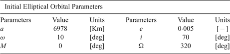
For the numerical simulations, the initial orbit parameters of the chief satellite are given in Table 2.
Initial elliptical orbital parameters

The inertia tensor of the deputy satellite is assumed to be J2d = diag([49, 55, 63] kg · m 2), and the position of the Position Sensing Diode sensor (feature point) is assumed to be P′ = [0 · 3, 0 · 3, 0 · 3] T metres in the BF frame. The sampling interval is set as Δt = 0 · 5s. In addition, the initial conditions for true/estimated position and velocity of the deputy's CM relative to the chief's CM are given, respectively:
 $$\eqalign{\rho_{o}\lpar t_{0}\rpar &= \lsqb 200\comma \; 200\comma \; 100\rsqb ^{T}\ m\comma \; \ v_{o} \lpar t_{0}\rpar = \lsqb 0{\cdot}01\comma \; v_{y} \lpar t_{0}\rpar \comma \; 0{\cdot}01\rsqb ^{T}\comma \; \ v_{y} \lpar t_0\rpar = \displaystyle{{-\dot{\theta }\lpar 2 + e\rpar } \over {\sqrt {\lpar 1 + e\rpar {\lpar 1-e\rpar }^3} }}\, x\lpar t_0\rpar \cr \tilde{\rho}_{o} \lpar t_{0}\rpar &= \lsqb 205\comma \; 205\comma \; 105\rsqb ^{T}\ m\comma \; \ \tilde{v}_{0} \lpar t_{0}\rpar \, {=}\, \lsqb 0{\cdot}011\comma \; \tilde{v}_{y} \lpar t_0\rpar \comma \; 0{\cdot}011\rsqb ^{T}\comma \; \ \tilde{v}_{y}\lpar t_0\rpar \, {=}\, \displaystyle{{-\dot{\theta }\lpar 2 + e\rpar } \over {\sqrt {\lpar 1 + e\rpar \lpar 1-e\rpar } }}\, \tilde{x}\lpar t_0\rpar } $$
The four beacons fixed on the chief are assumed (Lu et al., Reference Lu, Xiaoqian and Arun2015a) at:
 $$\eqalign{B1 &= \lsqb 0{\cdot}5\semicolon \; 0{\cdot}5\semicolon \; 0{\cdot}5\rsqb m\comma \; B2 = \lsqb -0{\cdot}5\semicolon \; -0{\cdot}5\semicolon \; 0{\cdot}5\rsqb m \cr B3 &= \lsqb -0{\cdot}5\semicolon \; 0{\cdot}5\semicolon \; -0{\cdot}5\rsqb m\comma \; B4 = \lsqb 0{\cdot}5\semicolon \; -0{\cdot}5\semicolon \; -0{\cdot}5\rsqb m} $$
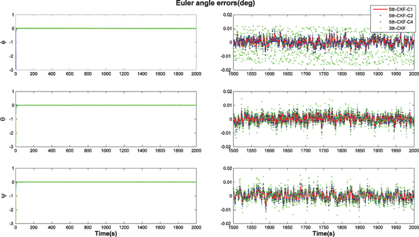
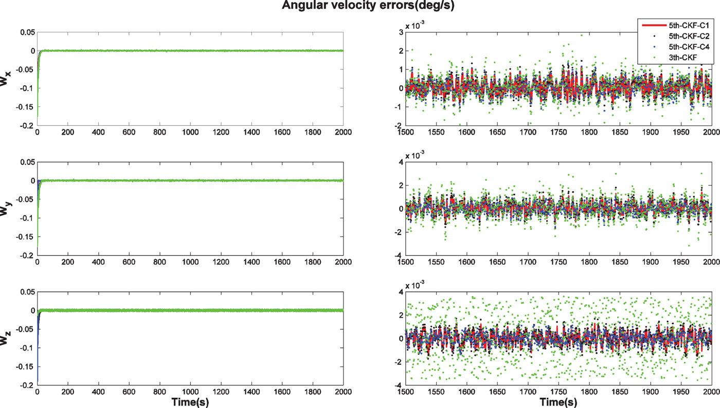
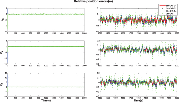
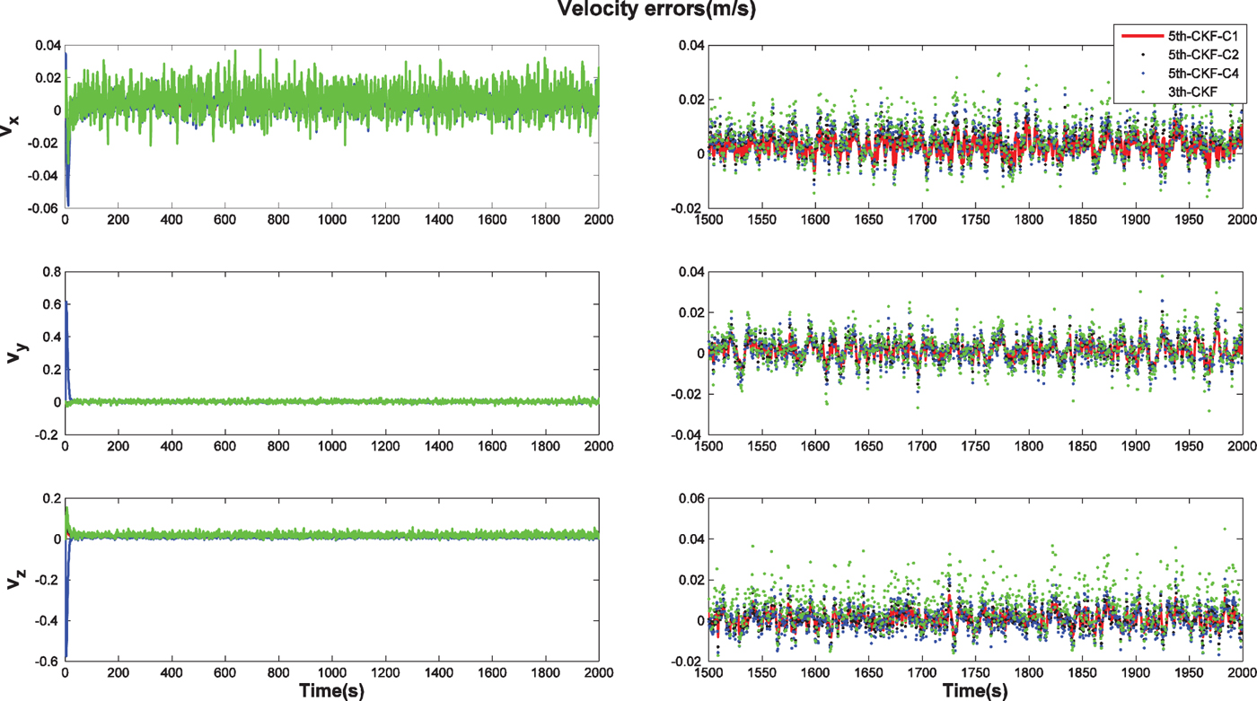
The simulation results of the proposed MRHCKF with fifth-degree/third-degree accuracy are depicted in Figures 1–4, showing the comparison between several MRHCKF, such as fifth-CKF-C1, fifth-CKF-C2 and fifth-CKF-C4 and third-CKF in all aspects of relative position and attitude. It is obvious that the original fifth-CKF with full state space has the best filtering performance for convergent accuracy. However, it has to use the largest number of sigma points at 289, which is its obvious disadvantage.
Relative Euler angular estimation errors.

Relative angular velocity estimation errors.

Relative position estimation errors.

Relative velocity estimation errors.

By introducing the multiple strategy to partition the state space, the fifth-CKF-C2, fifth-CKF-C4 and third-CKF has been also simulated to compare with the fifth-CKF-C1, which use 146 and 76 sigma-points, respectively. Evidently, the calculation burdens are reduced by factors of two and four times by the different partitioned subspaces, respectively, but, the performance degradations of estimation accuracy for the fifth-CKF-C2 and fifth-CKF-C4 are relatively limited. This characteristic can balance the filtering precision and computation burden for different requirements. In addition, the robust MRHCKF still has a better estimation performance than the traditional third-CKF, which also shows the advantages and application values of this work.
6. CONCLUSIONS
A series of Multiple Robust High-degree Cubature Kalman Filters (MRHCKF) are proposed by using the strategy of partitioning state space and the orthogonal principle, which can reduce the calculation burden for a high-dimension state system with high estimation accuracy. Then, a 6-DOF coupled dynamic model of relative position and attitude was reviewed and employed as the example for comparison between a traditional fifth-degree/third-degree CKF and the proposed MRHCKF. Finally, simulation results show that the proposed the MRHCKF can significantly reduce the amount of calculation with acceptable estimation accuracy, which could work well for relative state estimation of a spacecraft formation. It is clear that the method could be extended to other applications.
ACKNOWLEDGMENTS
This work was supported in part by the National Natural Science Foundation of China (51507140/51277150/51307140), the State Key Laboratory of Electrical Insulation and Power Equipment (EIPE17209), the Natural science special of Shaanxi Provincial Education Department (15JK1508), the Xi'an Beilin District Science and Technology Project (GX1622), the Guangdong Key Laboratory of Clean Energy Technology (2008A060301002), the Open Research Fund of Jiangsu Collaborative Innovation Center for Smart Distribution Network, the Nanjing Institute of Technology (XTCX201703) and the Specialized Research Fund for the Doctoral Program of Xi'an University of Technology (103-400211421).