




1 Introduction
It is believed that the lower mantle influences the Earth’s magnetic field by controlling the pattern of convection in the planet’s liquid core (Jones Reference Jones1977). The high-latitude patches of magnetic flux in the present-day field (Jackson, Jonkers & Walker Reference Jackson, Jonkers and Walker2000) suggest that lateral inhomogeneities in the heat flux at the lower mantle (Cox & Doell Reference Cox and Doell1964; Bloxham & Gubbins Reference Bloxham and Gubbins1987) possibly arising from mantle convection on long time scales (Yuen et al. Reference Yuen, Cadek, Chopelas and Matyska1993; Labrosse Reference Labrosse2002) can localize convection within the core. If the heat flux across the core–mantle boundary (CMB) is spatially inhomogeneous, core motions would be organized along preferred longitudes (e.g. Sumita & Olson Reference Sumita and Olson1999), in turn concentrating the inductively generated magnetic field.
The lateral variations in heat flux at the CMB can be correlated to variations in seismic shear wave velocity in the lower mantle (Williams, Revenaugh & Garnero Reference Williams, Revenaugh and Garnero1998; Masters et al. Reference Masters, Laske, Bolton, Dziewonski, Karato, Forte, Liebermann, Masters and Stixrude2000). The high-velocity zones of the mantle are considered to be denser than the regions of low velocity. Assuming a purely thermal origin for the density variation and a linear mapping of the velocity anomaly to heat flux variations, the resulting CMB thermal heterogeneity map shows a dominant twofold pattern in the spatial distribution of the heat flow (Willis, Sreenivasan & Gubbins Reference Willis, Sreenivasan and Gubbins2007), placing the lowest heat fluxes under the central Pacific and Africa, thought to be the sites of the mantle superplumes (Bréger & Romanowicz Reference Bréger and Romanowicz1998; Ritsema, van Heijst & Woodhouse Reference Ritsema, van Heijst and Woodhouse1999).
Mantle convection models (Nakagawa & Tackley Reference Nakagawa and Tackley2008; Olson et al. Reference Olson, Deguen, Rudolph and Zhong2015) indicate that the lateral variations in heat flux across the CMB can be at least twice the mean value at the boundary. Although geodynamo simulations (Olson & Christensen Reference Olson and Christensen2002; Takahashi et al. Reference Takahashi, Tsunakawa, Matsushima, Mochizuki and Honkura2008) suggest that large variations in CMB heat flux inhibit dynamo action, rapid rotation and weak core stratification (Sreenivasan & Gubbins Reference Sreenivasan and Gubbins2008) might alleviate this constraint.
Numerical models using lateral variation patterns described by spherical harmonics  $Y_{l}^{m}$ (Sun, Schubert & Glatzmaier Reference Sun, Schubert and Glatzmaier1994; Amit & Choblet Reference Amit and Choblet2009; Sahoo & Sreenivasan Reference Sahoo and Sreenivasan2017) have been extensively used to study thermal core–mantle coupling. With weak background rotation given by a relatively large Ekman number
 $E$, lateral variations arrest the motion of convection rolls that would otherwise drift eastwards (Zhang & Gubbins Reference Zhang and Gubbins1993). Here, the wavenumber of convection closely follows that of the applied lateral variation. When the wavenumber of convection is substantially larger than the wavenumber of the boundary heterogeneity, convection would likely be organized in localized clusters that satisfy the competing conditions set by rapid rotation and the lateral variation (Davies, Gubbins & Jimack Reference Davies, Gubbins and Jimack2009; Sreenivasan Reference Sreenivasan2009; Sahoo & Sreenivasan Reference Sahoo and Sreenivasan2017). A systematic study of rapidly rotating and strongly driven convection subject to large lateral variations in boundary heat flux is beyond the reach of present-day computers (although see Mound & Davies Reference Mound and Davies2017), and this provides the motivation to explore the problem through simplified laboratory experiments.
The centrifugal acceleration in rotating laboratory experiments resembles the component of planetary gravity perpendicular to the axis of rotation, but with opposite sign. Therefore, planetary core convection can be modelled in the laboratory by using the centrifugal acceleration with a reversed temperature gradient (Busse & Carrigan Reference Busse and Carrigan1976). The baroclinic flows that arise from the interaction between the Earth’s gravity  $\boldsymbol{g}$ and the mean horizontal temperature gradient has been noted in early experiments of rotating convection (Hide Reference Hide1958); however, the generation of these secondary flows can be minimized through rapid rotation (Boisson et al. Reference Boisson, Cébron, Moisy and Cortet2012). There are two obvious physical advantages of using a cylindrical annulus with sloping endwalls rather than a spherical annulus in the laboratory simulation of planetary convection. First, while the centrifugal acceleration of a spherical annulus interacts with the mean radial temperature gradient
 $\unicode[STIX]{x2202}T_{0}/\unicode[STIX]{x2202}r$ to produce azimuthal winds that are non-existent in the Earth’s core (Carrigan & Busse Reference Carrigan and Busse1983), these spurious flows are absent in a radially heated, rotating cylindrical annulus. Second, as we shall see in § 3.2, the quasi-geostrophic approximation used to model spherical shell convection outside the tangent cylinder (Busse Reference Busse1986; Gillet & Jones Reference Gillet and Jones2006) is satisfied even in strongly driven convection in a cylindrical annulus where the mean axial temperature gradient is
 $\unicode[STIX]{x2202}T_{0}/\unicode[STIX]{x2202}z=0$.
Because the component of gravity perpendicular to the axis of rotation makes the dominant contribution to buoyancy (Busse & Carrigan Reference Busse and Carrigan1976) and the heat flux variation on the Earth’s CMB is predominantly symmetric about the equator (e.g. Masters et al. Reference Masters, Laske, Bolton, Dziewonski, Karato, Forte, Liebermann, Masters and Stixrude2000), it is apparent that the azimuthal variation of the equatorial heat flux would control the structure of convection in the core. Motivated by this argument, a simplified experimental model is considered wherein convection in a rotating right cylindrical annulus is subject to purely azimuthal variations in outer boundary heat flux. The ratio of the centrifugal acceleration to Earth’s gravity, measured by the rotational Froude number, is  $9.26$, ensuring that the effective gravity is aligned with the radial temperature gradient. Owing to the absence of sloping endwalls, however, the Rossby wave-like drift of convection rolls (e.g. Azouni, Bolton & Busse Reference Azouni, Bolton and Busse1985) is absent in our experiment. Furthermore, the azimuthal wavenumber at convective onset in a spherical shell,
 $m_{c}\sim E^{-1/3}$ (where
 $E$ is the Ekman number that measures the ratio of viscous to Coriolis forces) (Carrigan & Busse Reference Carrigan and Busse1983; Cordero & Busse Reference Cordero and Busse1992), is independent of rotation in a cylindrical annulus (Zhang & Greed Reference Zhang and Greed1998). Despite the above differences between our annulus model and a spherical shell model, it is thought that the present experiment would be useful in understanding the patterns of convection formed at a fixed rotation rate and progressively increasing thermal forcing.
Laboratory experiments of rotating convection in a hemispherical shell with a heat source at the outer boundary (Sumita & Olson Reference Sumita and Olson1999, Reference Sumita and Olson2002) suggested that lower-mantle heterogeneities could substantially influence supercritical convection in the Earth’s core. A localized boundary heat source as used by Sumita & Olson could potentially produce large regions of stable stratification, a regime thought to be relevant to the core (Olson, Landeau & Reynolds Reference Olson, Landeau and Reynolds2017). The present study, on the other hand, confines itself to the regimes of unstable and neutrally stable stratification while focusing on the response of rotating convection to large-scale lateral variations in boundary heat flux.
The present experiment is further motivated by the probable role of the lower mantle in aiding the early geodynamo (Sahoo, Sreenivasan & Amit Reference Sahoo, Sreenivasan and Amit2016) as well as in the seismic anisotropy of the present-day inner core (e.g. Morelli, Dziewonski & Woodhouse Reference Morelli, Dziewonski and Woodhouse1986; Tanaka & Hamaguchi Reference Tanaka and Hamaguchi1997). The absence of chemical convection in early Earth’s core and the large estimates of the outer-core thermal conductivity (Pozzo et al. Reference Pozzo, Davies, Gubbins and Alfè2012; Hirose, Labrosse & Hernlund Reference Hirose, Labrosse and Hernlund2013) suggest that the thermal gradient may have been close to the adiabat. In our experiment, the influence of outer boundary heterogeneity on convection is understood from (a) the power input required for convective onset as a function of the magnitude of the heterogeneity ( $q^{\ast }$, defined by the ratio of variation in heat flux to the mean heat flux at the outer boundary), and (b) kinetic energy of the convective motions in the sectors of enhanced heat flux (see §§ 3.1 and 3.2). Furthermore, if the heterogeneity of the lower mantle is coupled with that of the inner core through the outer-core flow (Aubert et al. Reference Aubert, Amit, Hulot and Olson2008; Gubbins et al. Reference Gubbins, Sreenivasan, Mound and Rost2011), heat can flow into the inner core and cause localized melting while the average dominance of inner-core freezing would keep the dynamo active. In strongly supercritical convection, one would expect radial buoyancy to swamp the effect of the lateral variations (Sreenivasan & Gubbins Reference Sreenivasan and Gubbins2008), although a large
 $q^{\ast }$ can restore the coupling between the lower mantle and the inner core. As the regime of highly supercritical convection subject to large lateral variations has not received much attention in numerical simulations, we address the problem in § 3.4 by measuring the heat flux distribution at the inner boundary of the annulus in strongly driven convection at
 $q^{\ast }\approx 2$.
This paper is organized as follows. In § 2, the experimental set-up, the measurement plan and the relevant dimensionless parameters are presented. Then § 3 describes the experimental results, consisting of studies on the onset of convection, supercritical convection, generation of steady baroclinic flows with homogeneous and heterogeneous outer boundary heat flux, and the inner boundary heat flux variation. The implications of the results for planetary cores are discussed where appropriate. The main findings are summarized in § 4.
2 Experimental set-up
The experimental apparatus consists of a right circular cylindrical annulus of height 370 mm rotating about its vertical axis of symmetry. The schematic and photograph of the assembled set-up are shown in figure 1. The inner cylinder (IC) of radius  $r_{i}=50$ mm is made of 3 mm thick aluminium. The outer cylinder (OC) is made of 13 mm thick transparent poly(methyl methacrylate) (PMMA). The outer boundary of the annulus is at a radius
 $r_{o}=142$ mm. The gap width
 $L=92$ mm is taken as the characteristic length scale. To enable optical visualization, the 50 mm thick flat discs at the top and bottom are made of transparent PMMA; these discs also help to satisfy approximately insulating conditions at the two ends. A pair of axisymmetric grooves with rubber O-rings hold the outer and inner cylinders in place and prevents leakage of water, which is used as the working fluid in the experiment.
A coaxial stainless-steel shaft of 25 mm diameter, supported by a thrust bearing, rotates the experimental assembly. The shaft is driven by a 750 W direct-current servo-motor. The motor is controlled using a digitally operated electronic drive and has a feedback loop to maintain the rotation rate to within  $0.2\,\%$ of the set value. Thermal convection is produced by maintaining a temperature gradient across the annulus in the radial direction such that the IC is colder than the OC. The IC is maintained at a temperature of
 $22\,^{\circ }\text{C}$ with an accuracy of
 $0.1\,^{\circ }\text{C}$ by circulating water through it from a temperature-controlled bath using a fluid rotary union. A predetermined heat flux distribution is produced on the OC by passing a direct electric current via slip rings into an array of 0.4 mm Ni–Cr wires of resistance
 $30~\unicode[STIX]{x03A9}~\text{m}^{-1}$ wound on this cylinder. Figure 2 shows the heating circuit on the unfolded OC. The wire array is divided into four equal parts such that different currents can be passed through any of them, giving azimuthally varying heat flux. The difference in the currents is set by controlling the resistances R1 and R2 of the rheostats. To produce a onefold (approximately square-wave) pattern of heat flux heterogeneity, two adjacent parts are paired together to form a sector. For a twofold heterogeneity, two alternate parts are paired together so that diametrically opposite sectors have the same heat flux.
(a) Schematic and (b) photograph of the experimental set-up showing the important parts. All dimensions are in millimetres.

2.1 Instrumentation and data logging
The fluid velocity is measured by two-dimensional particle image velocimetry (PIV). The PIV system is co-rotated with the experiment in order to obtain velocities in the rotating frame. Water in the annulus is seeded with neutrally buoyant, silver-coated glass spheres (diameter 50  $\unicode[STIX]{x03BC}\text{m}$). As no radial motion of the particles is observed under rapid rotation, it is understood that there is no particle centrifugation. A horizontal cross-section of the annulus, whose plane is perpendicular to the rotation axis, is illuminated by a light sheet produced from an array of eight continuously driven solid-state diode lasers of power 1 W and wavelength 515–520 nm.
Two digital (GoPro 5) cameras each providing a  $180^{\circ }$ azimuthal field of view are used for image acquisition at a frame rate of 30 Hz and a pixel resolution of
 $1440\times 1080$ over an area
 ${\approx}300~\text{mm}\times 150~\text{mm}$. The hemispherical visual distortion in the recorded images is eliminated by fish-eye correction provided in the GoPro Studio software. The open-source software PIVlab (Thielicke & Stamhuis Reference Thielicke and Stamhuis2014) analyses the digital images to yield the velocity field. In this process, a digital image is first divided into coarse interrogation areas of
 $96\times 96$ pixels. Each interrogation area gives a single velocity vector derived from the cross-correlation of pixel intensity values for two consecutive images. Thus,
 $15\times 11$ vectors of
 $\boldsymbol{V}(x,y)$ are obtained over the entire area.
Schematic of the electrical system for generating azimuthally varying heat flux on the outer cylinder (OC). The array of Ni–Cr wires is divided into four sectors for twofold heating, each covering an azimuthal angle  $\unicode[STIX]{x1D719}=90^{\circ }$. The positive electrical terminals are denoted by P and the negative terminals are denoted by N. To obtain a onefold heating pattern, terminals N1 and N2 are disconnected from the Ni–Cr wires and terminals N3 and N4 are connected to N. Further, terminals P3 and P4 are disconnected from the slip ring and joined together. The higher current passes through the solid red wire and the lower current passes through the dotted blue wire. All dimensions are in millimetres.

The inner cylinder (IC) temperature is monitored using two temperature sensors (four-wire,  $100~\unicode[STIX]{x03A9}$ platinum resistance temperature detectors with an accuracy of
 $0.1\,^{\circ }\text{C}$) situated in the circulating fluid pipes just before the inlet and after the outlet (see figure 1). The measured temperature difference between the inlet and outlet does not exceed
 $0.2\,^{\circ }\text{C}$, implying an almost isothermal condition on the IC. To measure the heat flux into the annulus, 16 gSKIN thermopile sensors (of sensitivity
 $1.5~\unicode[STIX]{x03BC}\text{V}$ per
 $\text{W}~\text{m}^{-2}$) are affixed to the inside surface of the OC (
 $r=142~\text{mm}$). The lowest measurable difference in voltage of
 $0.6~\unicode[STIX]{x03BC}\text{V}$ gives a resolution of
 $0.41~\text{W}~\text{m}^{-2}$ for the measured heat flux. Data acquisition is done on-board via two PICOlog data loggers that convert the analogue signal to digital data at a frequency of 1 Hz. The distribution of the heat flux sensors on the OC surface is shown in figure 3(a,b). The measured heat flux is nearly uniform over the area on which it is imposed. The average heat flux is calculated by taking the spatial and temporal average of the measured heat flux values
 $$\begin{eqnarray}\frac{1}{N}\mathop{\sum }_{i=1}^{N}\langle Q_{i}\rangle _{t},\end{eqnarray}$$
where  $\langle \cdot \rangle _{t}$ denotes average over time and
 $N$ is the number of sensors. The variations of heat flux in time and space are given by the respective standard deviations,
 $\unicode[STIX]{x1D70E}_{x}$ and
 $\unicode[STIX]{x1D70E}_{t}$, from the mean surface heat flux
 $Q_{M}$, defined by
 $$\begin{eqnarray}\unicode[STIX]{x1D70E}_{x}=\sqrt{\frac{1}{N}\mathop{\sum }_{i}(Q_{i}-Q_{M})^{2}},\quad \unicode[STIX]{x1D70E}_{t}=\sqrt{\langle (Q_{i}-Q_{M})^{2}\rangle _{t}}.\end{eqnarray}$$
The relative deviations,
 $$\begin{eqnarray}\frac{\unicode[STIX]{x1D70E}_{x}}{Q_{M}}\times 100\,\%,\quad \frac{\unicode[STIX]{x1D70E}_{t}}{Q_{M}}\times 100\,\%,\end{eqnarray}$$
are within 1 % for input voltages in the range 0–80 V and do not exceed 5 % for voltages in the range 80–160 V. For inhomogeneous boundary heating, the mean heat flux  $Q_{M}$ in (2.3) is replaced by the sectoral mean heat flux (the quantities
 $Q_{A}$ and
 $Q_{B}$ in figure 3).
Figure 3(b) gives contours of the interpolated deviation of heat flux from the mean ( $\unicode[STIX]{x0394}Q=Q-Q_{M}$) for the onefold heterogeneity. The evolution in time of the measured heat flux (figure 3c) shows its bifurcation on the application of different electric currents to each sector at
 $t\approx 4500$ s, indicating the transition from the homogeneous to the heterogeneous heating pattern.
(a) Contours of the measured heat flux distribution  $Q$ for the case of homogeneous boundary heating. The mean surface heat flux,
 $Q_{M}=34.4~\text{W}~\text{m}^{-2}$. (b) Deviation of heat flux from the mean (
 $\unicode[STIX]{x0394}Q=Q-Q_{M}$) for a onefold heterogeneity pattern. The spatial locations of heat flux sensors are shown as black dots and the height
 $z$ is in millimetres. (c) Evolution of the measured heat flux with time (s) showing the transition from the homogeneous (a) to heterogeneous (b) states.

If  $Q_{A}$ and
 $Q_{B}$ are the average heat fluxes in two sectors, then the following conditions are satisfied in the experiment:
 $$\begin{eqnarray}\displaystyle & \displaystyle Q_{A}+Q_{B}=2Q_{M}, & \displaystyle\end{eqnarray}$$
 $$\begin{eqnarray}\displaystyle & \displaystyle |Q_{M}-Q_{A}|=|Q_{M}-Q_{B}|, & \displaystyle\end{eqnarray}$$
which ensure that (i) the mean heat flux is the same for both homogeneous and heterogeneous cases, and (ii) equal deviations from the mean heat flux are achieved in the two sectors. The magnitude of the heat flux heterogeneity is defined by the dimensionless number
 $$\begin{eqnarray}q^{\ast }=\frac{|Q_{A}-Q_{B}|}{Q_{M}}.\end{eqnarray}$$
From this definition, it is clear that the maximum value of  $q^{\ast }$ is 2, which for the onefold variation means that one of the sectors does not produce any heat flux (
 $Q_{A}=0$) while the other sector produces twice the mean heat flux (
 $Q_{B}=2Q_{M}$).
For homogeneous heating cases, the mean heat flux obtained from measurements lies below the ideal value estimated from Joule heating of the resistive wires (figure 4a), which indicates some loss of heat into the surroundings. For the onefold heterogeneity pattern, the equal deviations of the sectoral heat flux relative to the mean heat flux is evident from figure 4(b) and (c); notably, for  $q^{\ast }=2$, one of the sectors has approximately zero heat flux while the other has twice the mean heat flux. Values of
 $q^{\ast }>2$ necessitate strong stratification by controlled heat extraction from one or more sectors at the OC, which is not currently implemented in the experiment.
(a) Measured boundary heat flux averaged over space and time versus input voltage (green line) compared with the ideal values derived from Joule heating (black line) for homogeneous boundary heating ( $q^{\ast }=0$). The difference represents heat loss to the ambient air. (b) Average heat flux over the entire surface (green line), over the sector with heat flux higher than average (red line) and over the sector with heat flux lower than average (blue line) for onefold heterogeneity of magnitude
 $q^{\star }\approx 0.7$. (c) Plot similar to (b) for
 $q^{\star }\approx 2$.

2.2 Dimensionless parameters
Based on the scalings given in appendix A, the main dimensionless parameters in the experiment are the Ekman number  $E$, Rayleigh number
 $Ra$, rotational Froude number
 $Fr$ and Prandtl number
 $Pr$, defined as follows:
 $$\begin{eqnarray}E=\frac{\unicode[STIX]{x1D708}}{2\unicode[STIX]{x1D6FA}L^{2}},\quad Ra=\frac{\unicode[STIX]{x1D6FA}^{2}\unicode[STIX]{x1D6FC}\unicode[STIX]{x1D6FD}L^{5}}{\unicode[STIX]{x1D708}\unicode[STIX]{x1D705}},\quad Fr=\frac{\unicode[STIX]{x1D6FA}^{2}L}{g},\quad Pr=\frac{\unicode[STIX]{x1D708}}{\unicode[STIX]{x1D705}},\end{eqnarray}$$
where  $\unicode[STIX]{x1D708}$ is the kinematic viscosity,
 $\unicode[STIX]{x1D705}$ is the thermal diffusivity,
 $\unicode[STIX]{x1D6FC}$ is the thermal expansion coefficient,
 $\unicode[STIX]{x1D6FA}$ is the rotation rate,
 $L$ is the annulus width,
 $g$ is Earth’s gravity and
 $\unicode[STIX]{x1D6FD}$ is the temperature gradient at the outer boundary, determined by
 $$\begin{eqnarray}\unicode[STIX]{x1D6FD}=\left(\frac{\unicode[STIX]{x2202}T}{\unicode[STIX]{x2202}r}\right)_{r=r_{o}}=-\frac{Q_{M}}{k},\end{eqnarray}$$
with  $k$ being the thermal conductivity of water at 295 K. The experiments are performed at an Ekman number of
 $1.8\times 10^{-6}$ and a rotational Froude number of 9.26. The values (or ranges) of the main dimensionless parameters in the experiment are given in table 1.
Summary of the operating parameters in the experiment.

3 Experimental results
An experimental run begins by setting up rapid rotation of the annulus at constant angular velocity. Water from the constant-temperature bath is circulated through the IC so that its temperature remains approximately constant at 295 K. A heat flux pattern with the desired lateral variation is then applied on the exterior of the OC by controlling the electric current through the two rheostats (figure 2). When the measured heat flux becomes quasi-steady, flow visualization is done by illuminating a horizontal section by eight equispaced lasers. For a given  $q^{\ast }$,
 $Ra$ is increased in steps by increasing the mean heat flux through an enhanced voltage supplied to the heating element on the OC. For convection in a rotating cylindrical annulus, the horizontal (
 $r,\unicode[STIX]{x1D719}$) velocity is approximately invariant in the axial (
 $z$) direction (Zhang & Greed Reference Zhang and Greed1998; Alonso et al. Reference Alonso, Net, Mercader and Knobloch1999), which justifies the use of a two-dimensional planar PIV. We begin the study by examining the onset of convection in the annulus.
3.1 Onset of convection
Plots of horizontal velocity vectors (arrows) superposed on shaded contours of the  $z$ vorticity (
 $\text{s}^{-1}$) on a horizontal (
 $r,\unicode[STIX]{x1D719}$) plane at
 $z=180~\text{mm}$ for homogeneous outer boundary heat flux. (a) Experimentally obtained onset of convection with
 $Re_{peak}=59$,
 $Re_{rms}=14$,
 $Pe_{peak}=393$ and
 $Pe_{rms}=93$, where
 $Re$ and
 $Pe$ are the Reynolds and Péclet numbers. (b) Moderately supercritical convection with
 $Re_{peak}=127$,
 $Re_{rms}=65$,
 $Pe_{peak}=846$ and
 $Pe_{rms}=433$. (c) Numerically obtained convection near onset using temperature-dependent fluid properties
 $\unicode[STIX]{x1D708}$,
 $\unicode[STIX]{x1D705}$ and
 $\unicode[STIX]{x1D6FC}$ with
 $Re_{peak}=54$,
 $Re_{rms}=13$,
 $Pe_{peak}=361$ and
 $Pe_{rms}=86$. (d) Numerically obtained convection near onset using constant fluid properties with
 $Re_{peak}=49$,
 $Re_{rms}=34$,
 $Pe_{peak}=328$ and
 $Pe_{rms}=223$. The maximum velocity denoted by the longest arrow is
 $6.2\times 10^{-4}~\text{m}~\text{s}^{-1}$,
 $1.3\times 10^{-3}~\text{m}~\text{s}^{-1}$,
 $5.7\times 10^{-4}~\text{m}~\text{s}^{-1}$ and
 $5.1\times 10^{-4}~\text{m}~\text{s}^{-1}$ for plots (a), (b), (c) and (d), respectively.

Figure 5(a) shows the flow at onset of convection in the experiment with homogeneous outer boundary heat flux. The onset is determined by the minimum amount of heat flux required to obtain structures of the  $z$ vorticity that persist even when averaged over the entire period of measurement (360 s). Below this threshold, vortices may appear on short time scales, but do not show up on the time average. The structure of convection is that of small-scale cyclonic and anticyclonic columns, which appear close to the outer cylinder (figure 5a). Because these columns do not drift azimuthally, the flow at onset would be visible on long-time averages.
The three-dimensional direct numerical simulation of convective onset in the annulus, performed using a spectral element code (appendix B), is compared with the experimental onset. The no-slip condition for the velocity is imposed on all boundaries. As in the experiment, the heat flux is kept fixed at the outer cylinder and the inner cylinder is kept isothermal. For constant properties of the fluid, convection rolls extend across the annulus (figure 5d), in line with previous studies (King & Wilson Reference King and Wilson2005). However, the variation of the temperature along the radius  $r$ causes variation of the fluid properties
 $\unicode[STIX]{x1D708}$,
 $\unicode[STIX]{x1D6FC}$ and
 $\unicode[STIX]{x1D705}$, the variation of viscosity
 $\unicode[STIX]{x1D708}$ being the most appreciable. When a known empirical variation of these properties (Ahlers et al. Reference Ahlers, Brown, Araujo, Funfschilling, Grossmann and Lohse2006; Sugiyama et al. Reference Sugiyama, Calzavarini, Grossmann and Lohse2009; Horn & Shishkina Reference Horn and Shishkina2014) is included in the numerical model, the pattern of convective onset (figure 5c) matches closely with that in the experiment, suggesting that convection is preferentially excited at the periphery of the annulus where the viscosity is smallest. For the temperature difference at onset, the viscosity at the OC is estimated to be
 ${\approx}8\,\%$ lower than that at the IC. The peripheral onset is also noted for the onefold heat flux variation at the outer boundary (see figure 7a below), except that the convection is confined to the sector
 $\unicode[STIX]{x1D719}=[0,\unicode[STIX]{x03C0}]$ where the heat flux is higher than the mean. If the lowest measurable velocity in the experiment (
 ${\approx}1~\text{mm}~\text{s}^{-1}$) is set as the minimum onset velocity in the simulation, the onset Rayleigh numbers are in close agreement with each other. For comparison with the experiment, the Rayleigh number in the simulations (figure 5c,d) is set to the experimental value near onset,
 $3.9\times 10^{8}$. As
 $Ra$ is increased to
 $3\times Ra_{c}$ (
 $Ra_{c}$ being the critical Rayleigh number for onset) by enhancing the input heat flux, convection penetrates deep into the annulus (figure 5b), indicating improved homogeneity of temperature along the radius. The nearly axisymmetric anticyclonic flow and the accompanying ring of positive (red) vorticity near the IC (figure 5a) occur in the steady state from a thermal wind balance (see (3.5) below), irrespective of the presence or absence of convection. With deep convection, these thermal winds are present but not visible due to their relatively low magnitudes. The steady flows generated under homogeneous and heterogeneous outer boundary heat flux conditions are discussed in § 3.3.
An important issue is the value of the critical Rayleigh number for onset of convection, marked by the appearance of small-scale vortices, with heterogeneous boundary heat flux. Table 2 shows that the onset of convection for  $q^{\ast }>0$ requires much lower power input to the heating element than that for the case with homogeneous heat flux (
 $q^{\ast }=0$). The decrease in
 $Ra_{c}$ relative to its homogeneous value
 $Ra_{c,h}$ is measured by
 $$\begin{eqnarray}R^{\ast }={\displaystyle \frac{Ra_{c,h}-Ra_{c}}{Ra_{c,h}}}\times 100\,\%,\end{eqnarray}$$
which is given in table 2. The decrease in  $Ra_{c}$ with increasing
 $q^{\ast }$ is likely to result from the localized enhancement of the steady-state heat flux in the heterogeneous case relative to the homogeneous case (Sahoo & Sreenivasan Reference Sahoo and Sreenivasan2017). Therefore, we examine this deviation using the basic state solutions, obtained numerically by imposing a onefold heterogeneity pattern on the outer boundary (figure 19, appendix B) in subcritical (although unstably stratified) simulations at
 $Ra\ll Ra_{c}$ and different
 $q^{\ast }$. The heat flux deviation, shown in figure 6(a), is measured by
 $$\begin{eqnarray}R_{e}^{\ast }=\left\langle {\displaystyle \frac{Q(r,\unicode[STIX]{x1D719})-Q_{h}(r)}{Q_{h}(r)}}\right\rangle \times 100\,\%,\end{eqnarray}$$
where the subscript  $h$ refers to the homogeneous case and
 $\langle \cdot \rangle$ represents a horizontal surface average over the sector
 $[0,\unicode[STIX]{x03C0}]$ with inward heat flux greater than the mean value. Figure 6(b) shows a good agreement between
 $R_{e}^{\ast }$ with
 $R^{\ast }$, indicating that the decrease in the onset Rayleigh number for
 $q^{\ast }>0$ is adequately explained by the basic state heat flux deviation only (without convection). Table 2 also gives a local onset Rayleigh number (
 $Ra_{l}$) defined for the sector with enhanced heat flux, which does not decrease much with increasing
 $q^{\ast }$. The inference here is that the lowering of the threshold for onset is not experienced locally.
(a) Contour plot of the deviation in mean heat flux in the numerical basic state solution obtained by imposing a onefold heterogeneity pattern at the outer boundary. (b) Comparison of the experimental value  $R^{\star }$ given by (3.1) with the computed value
 $R_{e}^{\star }$ given by (3.2) for the onefold heterogeneity.

Experimental values of the total power input (W), critical Rayleigh number for onset of convection ( $Ra_{c}$), local Rayleigh number in the sector with heat flux higher than the mean (
 $Ra_{l}$), the decrease in percentage of the critical Rayleigh number relative to the homogeneous onset value (
 $R^{\ast }$), the estimated relative decrease in critical Rayleigh number (
 $R_{e}^{\ast }$) given by the heat flux deviation in the computed basic state (3.2), Reynolds number based on the peak velocity (
 $Re_{peak}$), Reynolds number based on the root-mean-square (r.m.s.) velocity (
 $Re_{rms}$) and Reynolds number based on the radial velocity component (
 $Re_{rms}^{rad}$).

3.2 Supercritical convection with laterally varying boundary heat flux
The measured velocity and vorticity fields for the onefold boundary heat flux pattern with a moderate variation  $q^{\ast }=0.7$ is given in figure 7. The plots are averaged over 360 s, which ensures reproducibility of the flow over realizations. (This period is
 ${\sim}20$ turnover times for the experiment, using the length scale 0.092 m and a characteristic peak velocity
 ${\sim}5\times 10^{-3}~\text{m}~\text{s}^{-1}$ for the range of Rayleigh numbers considered.) As for the case with homogeneous boundary heat flux, the onset rolls appear near the outer cylinder, but entirely in the sector with higher-than-average heat flux,
 $\unicode[STIX]{x1D719}=[0,\unicode[STIX]{x03C0}]$ (figure 7a). With higher power input, the rolls penetrate deeper into the annulus, but remain confined to the above sector (figure 7b). Further increase of the power input causes convection to start and then intensify in the sector of lower heat flux (figure 7c,d). The onset of convection in this sector occurs when the local Rayleigh number exceeds the critical value for the homogeneous case,
 $Ra_{c,h}$. Convection sets in near
 $\unicode[STIX]{x1D719}=0$ and
 $\unicode[STIX]{x1D719}=\unicode[STIX]{x03C0}/2$ only at higher
 $Ra$, probably because the radial temperature gradients at these locations are diminished by the azimuthal thermal winds that advect temperature from the sector with lower-than-average heat flux (see figure 15 below). For
 $Ra\approx 9Ra_{c}$, the effect of the lateral variation in the boundary heat flux is practically absent, indicating that the radial buoyancy has overcome the influence of the lateral variation.
Plots of the measured horizontal velocity vectors (arrows) superposed on shaded contours of the  $z$ vorticity (
 $\text{s}^{-1}$) on a horizontal (
 $r,\unicode[STIX]{x1D719}$) plane at
 $z=170~\text{mm }$ for the onefold heterogeneous heat flux pattern (
 $q^{\ast }\approx 0.7$). The boundary heat flux in the sector
 $\unicode[STIX]{x1D719}=[0,\unicode[STIX]{x03C0}]$ is higher than the mean value. The plots are averaged over a run time of 360 s. The onefold boundary heat flux pattern is indicated in panel (a), with the orange (green) outline showing higher (lower) heat flux than the average. The values of
 $Re_{peak}$,
 $Re_{rms}$,
 $Pe_{peak}$ and
 $Pe_{rms}$, in that order, are as follows: (a) 72, 20, 477, 131; (b) 98, 36, 648, 242; (c) 180, 76, 1194, 502; and (d) 216, 116, 1431, 773. The maximum velocity denoted by the longest arrow is
 $7.5\times 10^{-4}~\text{m}~\text{s}^{-1}$,
 $1\times 10^{-3}~\text{m}~\text{s}^{-1}$,
 $1.9\times 10^{-3}~\text{m}~\text{s}^{-1}$ and
 $2.2\times 10^{-3}~\text{m}~\text{s}^{-1}$ for (a), (b), (c) and (d), respectively.

For the onefold pattern with a high variation  $q^{\ast }\approx 2$, one sector
 $\unicode[STIX]{x1D719}=[0,\unicode[STIX]{x03C0}]$ has twice the mean heat flux, whereas the other sector
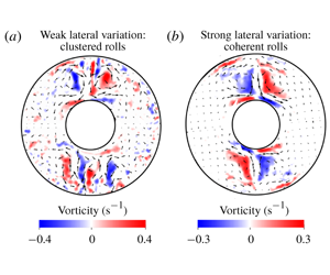
 $\unicode[STIX]{x1D719}=[\unicode[STIX]{x03C0},2\unicode[STIX]{x03C0}]$ has approximately zero heat flux and is therefore neutrally stable. Here, the clustered rolls at onset (figure 8a) give way to a coherent cyclone–anticyclone vortex pair slightly above onset (figure 8b). These coherent structures persist for still supercritical runs, the strongest forcing applied for this case being
 $Ra\approx 55.3Ra_{c}$. There is, however, no sign of convection in the neutrally stable sector.
Plots of the measured horizontal velocity vectors (arrows) superposed on shaded contours of the  $z$ vorticity (
 $\text{s}^{-1}$) on a horizontal (
 $r,\unicode[STIX]{x1D719}$) plane at
 $z=170$ mm for the onefold heterogeneous heat flux pattern (
 $q^{\ast }\approx 2$). The boundary heat flux in the sector
 $\unicode[STIX]{x1D719}=[0,\unicode[STIX]{x03C0}]$ is higher than the mean value. The plots are averaged over a run time of 360 s. The values of
 $Re_{peak}$,
 $Re_{rms}$,
 $Pe_{peak}$ and
 $Pe_{rms}$, in that order, are as follows: (a) 85, 25, 561, 164; (b) 125, 43, 833, 285. The maximum velocity denoted by the longest arrow is
 $8.8\times 10^{-4}~\text{m}~\text{s}^{-1}$ and
 $1.3\times 10^{-3}~\text{m}~\text{s}^{-1}$ for plots (a) and (b), respectively.

The coherent structures that form in supercritical convection are columns aligned with the rotation axis. A spatial correlation of  $z$ vorticity, defined by
 $$\begin{eqnarray}\frac{\overline{\unicode[STIX]{x1D714}_{1}\unicode[STIX]{x1D714}_{2}}}{\sqrt{\overline{\unicode[STIX]{x1D714}_{1}^{2}}\;\overline{\unicode[STIX]{x1D714}_{2}^{2}}}},\end{eqnarray}$$
between the two horizontal sections in figure 9 is 0.96. (Here,  $\unicode[STIX]{x1D714}_{1}$ and
 $\unicode[STIX]{x1D714}_{2}$ are the time-averaged vorticities measured at points on the two sections.) Even for the highest
 $Ra$ considered at this
 $q^{\ast }$ of 1.4 (
 $Ra=7.6\times 10^{9}$;
 ${\approx}38Ra_{c}$), the vorticity correlation is 0.85. The approximate axial invariance of the vorticity is understood from the
 $z$ component of the curl of the vorticity equation in the quasi-steady, inertia-free limit
 $$\begin{eqnarray}\frac{\unicode[STIX]{x2202}\unicode[STIX]{x1D714}_{z}}{\unicode[STIX]{x2202}z}={\displaystyle \frac{Ra\,E}{Fr}}\unicode[STIX]{x1D6FB}_{H}^{2}T+Ra\,E\left[2\frac{\unicode[STIX]{x2202}T}{\unicode[STIX]{x2202}z}+r\frac{\unicode[STIX]{x2202}^{2}T}{\unicode[STIX]{x2202}r\unicode[STIX]{x2202}z}\right]+E\unicode[STIX]{x1D6FB}^{4}u_{z},\end{eqnarray}$$
where  $\unicode[STIX]{x1D6FB}_{H}^{2}$ is the horizontal Laplacian. Since
 $\unicode[STIX]{x2202}T/\unicode[STIX]{x2202}z\approx 0$ in the experiment, the second term on the right-hand side of (3.4) is small. Furthermore, the small Ekman number
 $E$ and large rotational Froude number
 $Fr$ that result from rapid rotation ensure
 $\unicode[STIX]{x2202}\unicode[STIX]{x1D714}_{z}/\unicode[STIX]{x2202}z\approx 0$, which is the quasi-geostrophic approximation (Busse Reference Busse1986; Gillet & Jones Reference Gillet and Jones2006), often used to model rotating convection in spherical shells outside the tangent cylinder (Calkins Reference Calkins2018; Gastine Reference Gastine2019).
Plots of horizontal velocity vectors (arrows) superposed on  $z$ vorticity contours on two horizontal (
 $z$) sections located 100 mm above and below the midplane (
 $z=185$ mm). The lateral variation pattern is onefold of magnitude
 $q^{\ast }=1.4$ and
 $Ra=7.75\times 10^{8}$ (
 $3.9\times Ra_{c}$). The values of
 $Re_{peak}$,
 $Re_{rms}$,
 $Pe_{peak}$ and
 $Pe_{rms}$, in that order, are as follows: (a) 157, 66, 1041, 437; and (b) 164, 67, 1092, 448. The maximum velocity denoted by the longest arrow is
 $1.63\times 10^{-3}~\text{m}~\text{s}^{-1}$ and
 $1.71\times 10^{-3}~\text{m}~\text{s}^{-1}$ for plots (a) and (b), respectively.

The formation of the isolated downwelling between the coherent cyclone–anticyclone pair (figure 8b and figure 9) is reminiscent of the jet development noted at large  $q^{\ast }$ by Sumita & Olson (Reference Sumita and Olson1999, Reference Sumita and Olson2002) in their hemispherical shell experiments. However, the formation of a spiralling front that spans the annulus is prevented by the presence of the steady baroclinic flows of opposite sign, seen below in figure 15(b) (see also the spherical shell numerical simulations of Mound & Davies (Reference Mound and Davies2017)).
For the twofold pattern of heat flux variation at the outer boundary (figure 10), sectors A and C (orange outline) have enhanced heat flux while sectors B and D (green outline) have reduced heat flux relative to the mean value at the OC,  $Q_{M}$. The case
 $q^{\ast }\approx 1$ presents a series of convection patterns with increasing
 $Ra$. Convection sets in as a cluster of rolls near the outer boundary in the sectors of enhanced heat flux (figure 10a,b), as noted earlier for the onefold pattern. With increased heat input, convection penetrates radially inwards, and for
 $Ra\approx 2.5Ra_{c}$, two clusters of small-scale rolls elongated in the radial direction are produced (figure 10c). With further increase in
 $Ra$, the clusters give way to coherent pairs of cyclonic and anticyclonic vortices, which produce strong downwellings between them (figure 10d). These structures persist for a range of
 $Ra$ before the homogenization of convection begins at
 $Ra\approx 11.3Ra_{c}$, accompanied by the breakup of the coherent structures (figure 10e). Complete homogenization of convection occurs at
 $Ra\approx 23Ra_{c}$ (figure 10f), where there is no preferred azimuthal orientation of convection.
Plots of the measured horizontal velocity vectors (arrows) superposed on shaded contours of the  $z$ vorticity (
 $\text{s}^{-1}$) on a horizontal (
 $r,\unicode[STIX]{x1D719}$) plane at
 $z=180$ mm for the twofold heterogeneous heat flux pattern (
 $q^{\ast }\approx 1$) at progressively increasing
 $Ra$. The plots are averaged over a run time of 360 s. The twofold pattern is indicated in (a) with the orange (green) outline showing higher (lower) heat flux than the average. The values of
 $Re_{peak}$,
 $Re_{rms}$,
 $Pe_{peak}$ and
 $Pe_{rms}$ are, in that order, as follows: (a) 83, 26, 550, 169; (b) 132, 50, 875, 331; (c) 178, 84, 1179, 559; (d) 206, 106, 1370, 704; (e) 220, 128, 1460, 847; and (f) 226, 147, 1502, 976. The maximum velocity denoted by the longest arrow is
 $8.6\times 10^{-4}~\text{m}~\text{s}^{-1}$,
 $1.4\times 10^{-3}~\text{m}~\text{s}^{-1}$,
 $1.8\times 10^{-3}~\text{m}~\text{s}^{-1}$,
 $2.1\times 10^{-3}~\text{m}~\text{s}^{-1}$,
 $2.3\times 10^{-3}~\text{m}~\text{s}^{-1}$ and
 $2.4\times 10^{-3}~\text{m}~\text{s}^{-1}$ for plots (a)–(f), respectively.

For the twofold pattern with  $q^{\ast }\approx 2$, onset occurs as in figure 10(a); however, coherent cyclone–anticyclone vortex pairs appear in marginally supercritical convection and persist for a wide range of
 $Ra$ (figure 11a,b). At
 $Ra\approx 25Ra_{c}$, convection spills over to the neutrally stable sectors (figure 11c). At
 $Ra\approx 36Ra_{c}$, convection is completely homogenized in the annulus (figure 11d). For
 $q^{\ast }>2$, one would expect homogenization to occur at much higher
 $Ra$.
While it has been suggested that lateral thermal inhomogeneities that vary on the length scale of convection are not likely to affect the flow in the interior (Calkins et al. Reference Calkins, Hale, Julien, Nieves, Driggs and Marti2015), here we examine whether lateral variations of large magnitude wipe out convection at much smaller scales. By examining the flow averaged over a shorter time window of 54 s ( ${\sim}$3 turnover times), it is clear that the coherent structures are indeed accompanied by small scales (figure 12a,b) whose contribution to the dynamo process cannot be overlooked. While the long-lived coherent vortices concentrate magnetic flux in preferred longitudes (Willis et al. Reference Willis, Sreenivasan and Gubbins2007), the small scales continually generated by radial buoyancy can support the large-scale mean magnetic field (Moffatt Reference Moffatt1978; Sreenivasan & Gopinath Reference Sreenivasan and Gopinath2017).
Plots of the measured horizontal velocity vectors (arrows) superposed on shaded contours of the  $z$ vorticity (
 $\text{s}^{-1}$) on a horizontal (
 $r,\unicode[STIX]{x1D719}$) plane at
 $z=180$ mm for the twofold heterogeneous heat flux pattern (
 $q^{\ast }\approx 2$) at progressively increasing
 $Ra$. The plots are averaged over a run time of 360 s. The values of
 $Re_{peak}$,
 $Re_{rms}$,
 $Pe_{peak}$ and
 $Pe_{rms}$ are, in that order, as follows: (a) 171, 52, 1136, 343; (b) 237, 84, 1573, 560; (c) 312, 162, 2074, 1077; and (d) 327, 194, 2170, 1286. The maximum velocity denoted by the longest arrow is
 $1.8\times 10^{-3}~\text{m}~\text{s}^{-1}$,
 $2.5\times 10^{-3}~\text{m}~\text{s}^{-1}$,
 $3.2\times 10^{-3}~\text{m}~\text{s}^{-1}$ and
 $3.4\times 10^{-3}~\text{m}~\text{s}^{-1}$ for plots (a)–(d), respectively.

Plots of the measured horizontal velocity vectors (arrows) superposed on shaded contours of the  $z$ vorticity (
 $\text{s}^{-1}$) on a horizontal (
 $r,\unicode[STIX]{x1D719}$) plane at
 $z=180$ mm for the twofold heterogeneous heat flux pattern. The plots are averaged over a reduced time period of 54 s. The operating conditions (
 $q^{\ast },Ra$) are indicated above each panel. The values of
 $Re_{peak}$,
 $Re_{rms}$,
 $Pe_{peak}$ and
 $Pe_{rms}$, in that order, are as follows: (a) 244, 127, 1618, 845; and (b) 253, 91, 1679, 605. The maximum velocity denoted by the longest arrow is
 $2.5\times 10^{-3}~\text{m}~\text{s}^{-1}$ and
 $2.6\times 10^{-3}~\text{m}~\text{s}^{-1}$ for plots (a) and (b), respectively.

Figure 13 shows the r.m.s. value of the  $z$ vorticity calculated over the sector with enhanced heat flux. On time average, the persistence of convection rolls close to OC is reliably obtained when the vorticity intensity is
 ${\approx}0.1~\text{s}^{-1}$. This threshold is marked by the dashed horizontal line in the plots. The onset states, denoted by the filled symbols, indicate that the critical Rayleigh number decreases with increasing
 $q^{\ast }$. The ratio of r.m.s. values of the vorticities in the sectors with enhanced and diminished heat flux (
 $H$) is plotted against
 $Ra$ in figure 13(c,d). The regime
 $Ra\sim Ra_{c}$ is that for the occurrence of clustered rolls. The range of
 $Ra$ in which
 $H$ remains practically constant at a relatively small value is that of the coherent cyclone–anticyclone vortex pairs; notably, these vortices form for
 $q^{\ast }>1$. The start of homogenization is marked by the sharp increase in the value of
 $H$, which tends to unity for large
 $Ra$. The case
 $q^{\ast }=2$ for the onefold heterogeneity (blue line, figure 13c) is an exception, for convection does not homogenize here even at
 $Ra\approx 55Ra_{c}$.
(a,b) Variation of the r.m.s.  $z$ vorticity (
 $\widetilde{\unicode[STIX]{x1D714}}_{z}$, in
 $\text{s}^{-1}$) with Rayleigh number (
 $Ra$) in the sector with heat flux higher than the mean value. The case with homogeneous outer boundary heat flux (
 $q^{\ast }=0$) is also given. (c,d) The homogenization factor
 $H$, defined by the ratio of the r.m.s.
 $z$ vorticities in the sectors with enhanced and reduced heat flux.

The localization of convection by the inhomogeneous boundary heat flux may result in considerable enhancement of the kinetic energy in the sectors with higher heat flux than the average. The ratio  $E_{i}/E_{h}$ (where the subscripts i and h denote the inhomogeneous and homogeneous cases, respectively) of the kinetic energies has a high value
 ${\sim}$10–100 in moderately supercritical convection, but falls to a value
 ${\sim}$1 in the strongly driven regime (figure 14). However, for large lateral variations (
 $q^{\ast }>1$), a modest enhancement in local kinetic energy is noted even for high
 $Ra$.
It is notable that the presence of the coherent structures in the regime  $2\times 10^{8}<Ra<2\times 10^{9}$ and
 $q^{\ast }=2$ (figure 13b,d) corresponds to the regime of significant enhancement in the kinetic energy relative to the case of homogeneous outer boundary heat flux (figure 14b), along the lines of that found in the spherical shell simulation of Mound & Davies (Reference Mound and Davies2017) at
 $E\sim 10^{-4}$ and
 $q^{\ast }=5$, where the isolated narrow downwelling forms. Furthermore, their simulation shows an increase in the Nusselt number relative to the homogeneous case, which indicates that the regime of the coherent vortices is more efficient in the transport of heat across the shell than that of the roll clusters or that of homogenized convection.
Ratio of the total kinetic energy in the sector of enhanced heat flux to the respective energy in the homogeneous state ( $q^{\ast }=0$) plotted against Rayleigh number for the two patterns of heat flux heterogeneity (onefold and twofold) used in the experiment. The vertical line indicates the Rayleigh number where the ratio
 $E_{i}/E_{h}\approx 2$.

3.3 Steady mean flows with and without laterally varying boundary heat flux
In a thermally driven system, a no-flow steady state occurs when the temperature gradient is aligned with gravity. In the present experiment, this state, consisting of radial heating with the centrifugal acceleration acting as gravity, is violated by two factors: (i) Earth’s gravity acting in the negative  $z$ direction, and (ii) the imposed
 $\unicode[STIX]{x1D719}$ variation in boundary heat flux. In either case, the angle between the applied temperature gradient and gravity generates a baroclinic flow, also called the thermal wind.
The steady axisymmetric flow arising from the interaction between the radial temperature gradient and Earth’s gravity is described by (equation (A 8), appendix A)
 $$\begin{eqnarray}\frac{\unicode[STIX]{x2202}u_{\unicode[STIX]{x1D719}0}}{\unicode[STIX]{x2202}z}\approx {\displaystyle \frac{Ra\,E}{Fr}}\,\frac{\unicode[STIX]{x2202}T_{0}}{\unicode[STIX]{x2202}r},\end{eqnarray}$$
since  $\unicode[STIX]{x1D714}_{\unicode[STIX]{x1D719}}\approx 0$ in the experiment. As the mean inward heat flux decreases as
 $r^{-1}$, the value of
 $\unicode[STIX]{x2202}T_{0}/\unicode[STIX]{x2202}r$ peaks at the IC and decreases outwards. On a horizontal section below the cylinder midplane (
 $z=185$ mm), the baroclinic flow
 $u_{\unicode[STIX]{x1D719}0}$ is anticyclonic and is most prominent near the IC (figure 15a) in an experiment performed at
 $Ra=2.9\times 10^{8}$ (
 ${\approx}0.75Ra_{c}$). The numerical simulation at the same
 $Ra$ shows an identical mean flow near the IC (figure 15c). The ring of positive (red) mean
 $z$ vorticity seen in both the experiment and the simulation essentially follows the sign of
 $\unicode[STIX]{x2202}u_{\unicode[STIX]{x1D719}0}/\unicode[STIX]{x2202}r$.
Steady baroclinic flow field shown by horizontal velocity vectors (arrows) superposed on shaded contours of the  $z$ vorticity on a horizontal (
 $r,\unicode[STIX]{x1D719}$) section just below the midplane of the cylinder. (a) Experiment at
 $Ra=2.9\times 10^{8}$ (
 ${\approx}0.75Ra_{c}$) with homogeneous outer boundary heat flux. Here,
 $Re_{peak}=27$,
 $Re_{rms}=16$,
 $Pe_{peak}=179$ and
 $Pe_{rms}=104$. (b) Experiment at
 $Ra=9.7\times 10^{9}$ (
 ${\approx}55Ra_{c}$) with the onefold pattern of boundary heat flux at
 $q^{\ast }\approx 2$, averaged over a period of 900 s. Here,
 $Re_{peak}=33$,
 $Re_{rms}=24$,
 $Pe_{peak}=221$ and
 $Pe_{rms}=162$. (c) Numerical simulation at
 $Ra=2.9\times 10^{8}$ with homogeneous outer boundary heat flux. Here,
 $Re_{peak}=24$,
 $Re_{rms}=13$,
 $Pe_{peak}=158$ and
 $Pe_{rms}=89$. (d) Numerical simulation at
 $Ra=1.7\times 10^{7}$ with the onefold pattern of boundary heat flux. Here,
 $Re_{peak}=28$,
 $Re_{rms}=21$,
 $Pe_{peak}=188$ and
 $Pe_{rms}=136$. The maximum velocity denoted by the longest arrow is
 $2.8\times 10^{-4}~\text{m}~\text{s}^{-1}$,
 $3.5\times 10^{-4}~\text{m}~\text{s}^{-1}$,
 $2.5\times 10^{-4}~\text{m}~\text{s}^{-1}$ and
 $3.0\times 10^{-4}~\text{m}~\text{s}^{-1}$ for plots (a), (b), (c) and (d), respectively.

The case of the onefold heat flux heterogeneity at the outer boundary gives rise to a two-cell (cyclone–anticyclone) mean flow pattern (figure 15b). As remarked earlier, the oppositely signed mean flow cells sandwich the radial downwelling between them. This mean flow is too weak to be detected below onset (due to the inherent noise) as well as in supercritical regimes dominated by the coherent structures, so a highly supercritical state ( $Ra=9.7\times 10^{9}$) consisting of small-scale fluctuating convection needs to be averaged over a long time period of 900 s in order to recover the steady baroclinic flow. The numerical simulation with the onefold boundary pattern (figure 15d), on the other hand, produces a qualitatively similar flow field at a relatively small Rayleigh number (
 $Ra=1.7\times 10^{7}$) below onset. To understand the pattern of the mean
 $z$ vorticity
 $\unicode[STIX]{x1D714}_{z0}$ that peaks on either side of
 $\unicode[STIX]{x1D719}=\unicode[STIX]{x03C0}/2$, the evolution of
 $\unicode[STIX]{x2202}T_{0}/\unicode[STIX]{x2202}\unicode[STIX]{x1D719}$ in the simulation is tracked from its initial state (figure 16a), derived from the solution of
 $\unicode[STIX]{x1D6FB}^{2}T_{0}=0$. The mean flow, shown by the arrows in figure 15(d), advects this temperature field, so that the steady-state structure of
 $\unicode[STIX]{x2202}T_{0}/\unicode[STIX]{x2202}\unicode[STIX]{x1D719}$ (figure 16b) is closely followed by
 $\unicode[STIX]{x1D714}_{z0}$. The growth of vorticity is fed by the azimuthal variation in temperature and limited by viscous diffusion, yielding the steady-state balance
 $$\begin{eqnarray}Ra{\displaystyle \frac{\unicode[STIX]{x2202}T_{0}}{\unicode[STIX]{x2202}\unicode[STIX]{x1D719}}}+\unicode[STIX]{x1D6FB}^{2}\unicode[STIX]{x1D714}_{z0}=0,\end{eqnarray}$$
which is different from the buoyancy–Coriolis force balance expected for the steady state in rotating spherical shells.
Plots of the azimuthal variation in the mean temperature,  $\unicode[STIX]{x2202}T_{0}/\unicode[STIX]{x2202}\unicode[STIX]{x1D719}$, at the starting and saturated states of the numerical simulation of the basic state with the onefold heterogeneity pattern in boundary heat flux. The Rayleigh number in the simulation,
 $Ra=1.7\times 10^{7}$, is well below the onset value.

3.4 Heat flux variation on the inner cylinder
Over a wide range of  $Ra$, the convection at large
 $q^{\ast }$ is characterized by cyclone–anticyclone vortex pairs and their attendant downwellings beneath regions of enhanced heat flux. Motivated by the idea that outer-core convection can cause inhomogeneity in heat flux at the inner-core boundary (ICB), the heat flux distribution at the IC is measured by affixing heat flux sensors to its surface. Figure 17 shows the inward heat flux map at the IC for the twofold heterogeneity pattern at
 $q^{\ast }\approx 2$. The region
 $\unicode[STIX]{x03C0}/4\leqslant \unicode[STIX]{x1D719}\leqslant 5\unicode[STIX]{x03C0}/4$ is shown, which encompasses two adjacent sectors, one of enhanced heat flux and the other of diminished (nearly zero) heat flux at the OC. In order to obtain a well-resolved heat flux distribution at the IC, 16 heat flux sensors are placed on two adjacent sectors at a time. Below onset of convection (figure 17a), the heat flux is approximately that derived from the steady basic state temperature distribution in the annulus. Here, the peak IC heat flux of
 ${\approx}32~\text{W}~\text{m}^{-2}$ is greater than the peak OC flux of
 ${\approx}12~\text{W}~\text{m}^{-2}$ by the geometric factor
 $r_{o}/r_{i}$ (equation (B 1), appendix B). Above onset, the dichotomy between the two sectors is pronounced: the narrow downwellings concentrate the patch of enhanced heat flux while regions of reversed heat flux develop in the sector of low heat flux (figure 17b,c). As
 $Ra$ is increased further, a narrow band of intense (red) heat flux and a broad region of reversed (blue) heat flux form (figure 17d) and persist until
 $Ra\approx 20Ra_{c}$. This local intensification of heat flux on the inner boundary is caused by the impingement of the jet-like downwelling concentrated at this azimuthal location, also indicated by spherical shell dynamo simulations at marginally supercritical convection and
 $q^{\ast }<1$ (Gubbins et al. Reference Gubbins, Sreenivasan, Mound and Rost2011). Because the direction of gravity and that of the heat flow in the experiment are both opposite to that in Earth, it is apparent that the narrow red band would represent regions that favour inner-core freezing, whereas the broad region of reversed flux may cause melting. For
 $Ra>20Ra_{c}$, convection spills over into the neutrally stable sector (see figure 11c), which eventually leads to the homogenization of the IC heat flux (figure 17e,f). For
 $q^{\ast }>2$, one would expect the regime of strong heat flux dichotomy to last for much higher
 $Ra$ (
 $Ra/Ra_{c}\gg 10$) before homogenization sets in.
At this point, we recall that the organization of core convection in preferred longitudes may give rise to the high-latitude flux lobes in present-day Earth’s magnetic field (Gubbins, Willis & Sreenivasan Reference Gubbins, Willis and Sreenivasan2007; Willis et al. Reference Willis, Sreenivasan and Gubbins2007). Therefore, supercritical convection at large  $q^{\ast }$ can account for the high-latitude CMB magnetic flux patches as well as the lateral variations in seismic P-wave velocity in the outermost inner core (e.g. Bergman Reference Bergman1997). A previous study (Aubert, Finlay & Fournier Reference Aubert, Finlay and Fournier2013) relates the mass flux heterogeneity on Earth’s ICB to the concentration of CMB magnetic flux through a numerical model having
 $E\sim 10^{-5}$ and an imposed inner boundary heterogeneity of magnitude 0.8. The present study, on the other hand, proposes that a large azimuthal variation in the CMB heat flux by itself can produce the inner-core heterogeneity via inhomogeneous outer-core convection.
Shaded contours of the measured heat flux at the IC for the twofold heat flux heterogeneity pattern at  $q^{\ast }\approx 2$. The region
 $\unicode[STIX]{x03C0}/4\leqslant \unicode[STIX]{x1D719}\leqslant 5\unicode[STIX]{x03C0}/4$ is shown, which consists of two adjacent sectors of enhanced and diminished (
 ${\approx}$0) OC heat flux. The Rayleigh number for each run is given above the respective panel. The location of the 16 heat flux sensors (black dots) are shown in (a). A similar pattern of the heat flux is obtained over the other two sectors.

Figure 18 gives the extremum values of the measured IC heat flux in the sectors of enhanced (red) and diminished (blue) heat input. Computations using Nek5000 (appendix B) of the steady basic state for Rayleigh numbers below onset indicate that the basic state heat flux would scale linearly with  $Ra$; therefore, its value in supercritical experiments is estimated by linearly scaling up the measured IC heat flux for the lowest
 $Ra$. In the sector of enhanced heat input, the measured IC heat flux is consistently higher than the basic state value. Curiously, in the sector of nearly zero heat input, the measured IC heat flux falls below the basic state and even reverses direction, as noted earlier in figure 17(d). The measured heat flux exceeds the basic state only for
 $Ra>4\times 10^{9}$, when homogenization sets in (see figure 11c). Figure 18 shows that convection markedly amplifies the dichotomy in IC heat flux between the two sectors, thus providing a regime conducive to localized melting and freezing of the Earth’s inner core. For values of
 $q^{\ast }>2$, one would reasonably expect higher magnitudes of the reversed IC heat flux over a wider range of
 $Ra$, resulting in a stronger dichotomy in the sectoral heat flux.
Extremum (peak) values of the measured IC heat flux for the twofold heat flux heterogeneity pattern at  $q^{\ast }\approx 2$. The sectors with enhanced heat input (red symbols) and diminished (
 ${\approx}0$) heat input (blue symbols) are shown separately. The solid lines give the linearly scaled estimate of the steady basic state heat flux for comparison.

4 Conclusion
The present study of rotating convection subject to lateral variations in boundary heat flux is largely motivated by the influence of the lower mantle on outer-core convection in the Earth. The cylindrical geometry and the purely azimuthal variation in the applied boundary heat flux ensure that the experiments satisfy the quasi-geostrophic approximation even in highly supercritical states. Although the azimuthal length scale at convective onset in a cylindrical annulus is independent of rotation (Zhang & Greed Reference Zhang and Greed1998), the patterns of convection in strongly driven, approximately geostrophic states are obtained in the experiment. Convection at onset or in mildly supercritical states takes the form of roll clusters confined to the sectors of enhanced heat flux, provided  $q^{\ast }\lesssim 1$ (figure 10). The long-lived structure of convection at
 $q^{\ast }>1$ is that of coherent cyclone–anticyclone vortex pairs, which produce narrow downwellings between them. The occurrence of coherent vortices has been noted in rotating plane layer convection models (see Guervilly & Hughes Reference Guervilly and Hughes2017; Julien, Knobloch & Plumley Reference Julien, Knobloch and Plumley2018; Favier, Guervilly & Knobloch Reference Favier, Guervilly and Knobloch2019). Our experiments with
 $q^{\ast }>1$ show that the coherent vortices coexist with organized small-scale convection beneath regions of enhanced boundary heat flux (figure 12) on short time scales. On the other hand, our experiments with
 $q^{\ast }<1$ show the confinement of small-scale convection rolls (figure 7), supported by spherical shell numerical models with
 $q^{\ast }<1$ (Davies et al. Reference Davies, Gubbins and Jimack2009; Dietrich, Hori & Wicht Reference Dietrich, Hori and Wicht2016).
The input power requirement for onset of convection (also measured by the critical Rayleigh number  $Ra_{c}$) for
 $q^{\ast }=2$ decreases by
 ${\sim}50\,\%$ relative to its value with homogeneous boundary heat flux (table 2), which can be explained by the deviations of the basic state (steady) heat flux from the mean value (see Sahoo & Sreenivasan (Reference Sahoo and Sreenivasan2017) for a comparable result in spherical shells).
For  $q^{\ast }\approx 2$, convection does not occur via the onset route in the neutrally stable sector (of zero OC heat flux) even in the strongly supercritical experiments. With the twofold heterogeneity pattern, convection is fully homogenized at
 $Ra\approx 36Ra_{c}$ probably via advection of the temperature perturbations by the mean flow into the ‘quiescent’ sectors of zero OC heat flux, a process that does not seem to occur with the onefold pattern. Here, the baroclinic flow arising from the interaction between the steady-state temperature gradient
 $\unicode[STIX]{x2202}T_{0}/\unicode[STIX]{x2202}\unicode[STIX]{x1D719}$ and the centrifugal acceleration is weak in the quiescent sector
 $\unicode[STIX]{x1D719}=[\unicode[STIX]{x03C0},2\unicode[STIX]{x03C0}]$ (figure 15b,d) and is therefore unable to carry convection into this sector. If the high-latitude magnetic flux patches in the present-day geomagnetic field are taken to be the signature of an inhomogeneously convecting core, one might argue that the value of
 $q^{\ast }$ at the CMB should be much higher than 2. However, further investigation in the high-
 $Ra$, high-
 $q^{\ast }$ regime in spherical shells is needed to adequately support this hypothesis.
If the mean heat flux at the Earth’s CMB is close to the adiabatic heat flux (Anufriev, Jones & Soward Reference Anufriev, Jones and Soward2005; Pozzo et al. Reference Pozzo, Davies, Gubbins and Alfè2013), the value of  $q^{\ast }$ can be very large. Here, lateral variations in the heat flux would likely produce regions of subadiabatic heat flux beneath the CMB (e.g. Olson et al. Reference Olson, Landeau and Reynolds2017), which have not been simulated in the present experiment. As the adiabatic reference state is close to that of uniform temperature in the Boussinesq limit, any measured heat flux in the experiment may be considered to be superadiabatic. Values of
 $q^{\ast }>2$ require controllable heat sinks on the OC, which would be implemented as part of a future study.
The occurrence of localized coherent vortices at  $Ra\gg Ra_{c}$ and
 $q^{\ast }\approx 2$ led to the exploration of the inner boundary heat flux heterogeneity in this parameter regime. The measured heat flux variation at the IC is considerably larger compared to that at the OC. The heat flux map derived from the seismic shear wave velocity variation in the lower mantle shows deviations from the idealized twofold pattern of heat flux near the equator: for example, the fluxes beneath Central America and south India are not equal. Because the interaction between the lateral buoyancy and Earth’s gravity is maximum at the equator, the variations in core flow produced by these differences in heat flux are probably well understood from cylindrical annulus experiments.
In the light of this study, it would be interesting to explore the following phenomena in spherical shell dynamo models: (a) the homogenization of convection at  $Ra\gg Ra_{c}$ and with large values of
 $q^{\ast }$ that would produce subadiabatic regions beneath the CMB, (b) generation of the axial dipole magnetic field at large
 $q^{\ast }$ and low
 $E$, which would otherwise be inhibited due to loss of geostrophy of the convection, and (c) the natural occurrence of the
 $m=1$ heterogeneity pattern on the ICB due to the lower-mantle heat flux heterogeneity derived from the seismic shear wave velocity variation.
Acknowledgements
B.S. was awarded a SwarnaJayanti fellowship by the Department of Science and Technology (India) during this project. This study was supported in part by Research Grant no. 5307-1 awarded by the Indo-French Centre for the Promotion of Advanced Research (IFCPAR). The authors acknowledge the help of Ghanesh Narasimhan in designing the experimental set-up.
Appendix A. Governing equations for convection in a rotating cylindrical annulus
The dimensional equations of momentum, energy and mass conservation are given by
 $$\begin{eqnarray}\displaystyle & \displaystyle \frac{\unicode[STIX]{x2202}\boldsymbol{u}}{\unicode[STIX]{x2202}t}+(\boldsymbol{u}\boldsymbol{\cdot }\unicode[STIX]{x1D735})\boldsymbol{u}+2\unicode[STIX]{x1D6FA}\,\hat{\boldsymbol{e}}_{z}\times \boldsymbol{u}=-\frac{\unicode[STIX]{x1D735}p}{\unicode[STIX]{x1D70C}}+g\unicode[STIX]{x1D6FC}\,T\hat{\boldsymbol{e}}_{z}-\unicode[STIX]{x1D6FA}^{2}\unicode[STIX]{x1D6FC}\,T\boldsymbol{r}+\unicode[STIX]{x1D735}\boldsymbol{\cdot }(\unicode[STIX]{x1D708}\,\unicode[STIX]{x1D735}\boldsymbol{u}), & \displaystyle\end{eqnarray}$$
 $$\begin{eqnarray}\displaystyle & \displaystyle \unicode[STIX]{x1D70C}c_{p}\left(\frac{\unicode[STIX]{x2202}T}{\unicode[STIX]{x2202}t}+\boldsymbol{u}\boldsymbol{\cdot }\unicode[STIX]{x1D735}T\right)=\unicode[STIX]{x1D735}\boldsymbol{\cdot }(\unicode[STIX]{x1D705}\unicode[STIX]{x1D735}T), & \displaystyle\end{eqnarray}$$
 $$\begin{eqnarray}\displaystyle & \displaystyle \unicode[STIX]{x1D735}\boldsymbol{\cdot }\boldsymbol{u}=0, & \displaystyle\end{eqnarray}$$
where  $\unicode[STIX]{x1D6FA}$ is the rotation rate,
 $\unicode[STIX]{x1D708}$ is the kinematic viscosity,
 $\unicode[STIX]{x1D705}$ is the thermal diffusivity,
 $c_{p}$ is the specific heat at constant pressure and
 $\unicode[STIX]{x1D6FC}$ is the coefficient of thermal expansion. For constant diffusivities, the equations in dimensionless form are obtained by scaling lengths by the annulus width
 $L$, velocity
 $u$ by
 $\unicode[STIX]{x1D705}/L$, time
 $t$ by
 $L^{2}/\unicode[STIX]{x1D705}$, pressure
 $p$ by
 $\unicode[STIX]{x1D70C}u^{2}$ and temperature
 $T$ by
 $\unicode[STIX]{x1D6FD}L$, where
 $\unicode[STIX]{x1D6FD}$ is the radial temperature gradient at the outer boundary:
 $$\begin{eqnarray}\displaystyle & \displaystyle \frac{E}{Pr}\left(\frac{\unicode[STIX]{x2202}\boldsymbol{u}}{\unicode[STIX]{x2202}t}+(\unicode[STIX]{x1D735}\times \boldsymbol{u})\times \boldsymbol{u}\right)+\hat{\boldsymbol{e}}_{z}\times \boldsymbol{u}=-\unicode[STIX]{x1D735}p^{\ast }+\frac{Ra\,E}{Fr}\,T\,\hat{\boldsymbol{e}}_{z}\,-Ra\,E\,T\boldsymbol{r}+E\,\unicode[STIX]{x1D6FB}^{2}\boldsymbol{u}, & \displaystyle \nonumber\\ \displaystyle & & \displaystyle\end{eqnarray}$$
 $$\begin{eqnarray}\displaystyle & \displaystyle \frac{\unicode[STIX]{x2202}T}{\unicode[STIX]{x2202}t}+(\boldsymbol{u}\boldsymbol{\cdot }\unicode[STIX]{x1D735})T=\unicode[STIX]{x1D6FB}^{2}T, & \displaystyle\end{eqnarray}$$
 $$\begin{eqnarray}\displaystyle & \displaystyle \unicode[STIX]{x1D735}\boldsymbol{\cdot }\boldsymbol{u}=0, & \displaystyle\end{eqnarray}$$
where  $p^{\ast }=p+\frac{1}{2}E\,Pr^{-1}|\boldsymbol{u}|^{2}$ and the non-dimensional numbers are defined by
 $$\begin{eqnarray}E=\frac{\unicode[STIX]{x1D708}}{2\unicode[STIX]{x1D6FA}L^{2}},\quad Ra=\frac{\unicode[STIX]{x1D6FA}^{2}\unicode[STIX]{x1D6FC}\unicode[STIX]{x1D6FD}L^{5}}{\unicode[STIX]{x1D708}\unicode[STIX]{x1D705}},\quad Fr=\frac{\unicode[STIX]{x1D6FA}^{2}L}{g},\quad Pr=\frac{\unicode[STIX]{x1D708}}{\unicode[STIX]{x1D705}}.\end{eqnarray}$$
Of particular interest in this study is the inertia-free limit that results from rapid rotation, where the steady (basic state) flow is governed by the time-averaged vorticity equation
 $$\begin{eqnarray}-\frac{\unicode[STIX]{x2202}\boldsymbol{u}_{0}}{\unicode[STIX]{x2202}z}=\frac{Ra\,E}{Fr}\,(\unicode[STIX]{x1D735}\times T_{0}\,\hat{\boldsymbol{e}}_{z})-Ra\,E\,(\unicode[STIX]{x1D735}\times T_{0}\,\boldsymbol{r})+E\,\unicode[STIX]{x1D6FB}^{2}\unicode[STIX]{x1D74E}_{0},\end{eqnarray}$$
where  $\unicode[STIX]{x1D74E}$ is the vorticity and the subscript ‘0’ refers to the basic state.
Appendix B. Numerical model
A numerical model that mimics the laboratory experiment is set up using the code Nek5000 (Fischer, Lottes & Kerkemeier Reference Fischer, Lottes and Kerkemeier2008). The domain is a cylindrical annulus with flat top and bottom ends, the spatial dimensions of which are the same as that for the experiment. The dimensional equations (A 1)–(A 3) are solved using the variable properties  $\unicode[STIX]{x1D708}$,
 $\unicode[STIX]{x1D6FC}$ and
 $\unicode[STIX]{x1D705}$ whose temperature dependence is known (Ahlers et al. Reference Ahlers, Brown, Araujo, Funfschilling, Grossmann and Lohse2006; Sugiyama et al. Reference Sugiyama, Calzavarini, Grossmann and Lohse2009; Horn & Shishkina Reference Horn and Shishkina2014). The inner cylinder is isothermal while the outer cylinder has a known heat flux imposed on it.
The Nek5000 code uses a spectral element method to discretize the governing equations. The annular computational domain is divided into  $N_{E}$ = 13 440 hexahedral elements with 28, 32 and 15 elements in the
 $r$,
 $\unicode[STIX]{x1D719}$ and
 $z$ directions, respectively. Within each element, the velocity and temperature are represented as the tensor-product Lagrange polynomials of orders
 $N_{p}$ located at the Gauss–Lobatto–Legendre points, while pressure is represented by
 $N_{p}-2$ polynomials based at Gauss–Legendre points. The degrees of freedom scale as
 $N_{E}\times N_{p}^{3}$. The numerical convergence is algebraic with the number of elements
 $N_{E}$ and exponential with the polynomial order
 $N_{p}$. A third-order implicit backward differencing scheme is used for spatial discretization. The spectral order
 $N_{p}=8$ and the 3/2 dealiasing rule are used to accurately compute the nonlinear terms. The code is MPI-parallelized and has been shown to scale efficiently for up to
 $10^{6}$ processors (Offermans et al. Reference Offermans, Marin, Schanen, Gong, Fischer, Schlatter, Obabko, Peplinski, Hutchinson and Merzari2016). The simulations were performed on the SahasraT, the supercomputer at IISc Bangalore on typically 1680 processors.
The numerical model was benchmarked against the results from Alonso et al. (Reference Alonso, Net, Mercader and Knobloch1999). In their model, a vertically rotating cylindrical annulus is heated radially in the presence of an imposed constant radial gravity. The properties of the fluid are assumed to be independent of temperature. The case for Taylor number  $Ta=E^{-2}=10^{7}$,
 $\unicode[STIX]{x1D702}=r_{i}/r_{o}=0.35$ and
 $Pr=0.7$ is considered with no-slip boundaries (figure 5a in their paper). The critical parameters for the onset of convection obtained in the simulation (with their values in brackets) are the Rayleigh number
 $Ra_{c}=2640$ (
 ${\approx}2600$) and wavenumber
 $n=3$ (
 $3$).
For  $Ra<Ra_{c}$, the code reproduces the basic state temperature profile with homogeneous outer boundary heat flux
 $Q_{M}$,
 $$\begin{eqnarray}T(r)=T_{i}+\unicode[STIX]{x1D6FD}r_{o}\ln (r/r_{i}),\end{eqnarray}$$
where
 $$\begin{eqnarray}\unicode[STIX]{x1D6FD}=\left(\frac{\unicode[STIX]{x2202}T}{\unicode[STIX]{x2202}r}\right)_{r=r_{o}}=-\frac{Q_{M}}{k}.\end{eqnarray}$$
The pattern of onefold boundary heat flux variation in the experiment is approximated by the following distribution (figure 19):
 $$\begin{eqnarray}Q=\tanh \left(\frac{\sin \unicode[STIX]{x1D719}}{\unicode[STIX]{x1D6FF}}\right),\end{eqnarray}$$
where  $\unicode[STIX]{x1D6FF}=0.2$.
Boundary heat flux condition in the numerical simulation that approximates the onefold (approximately square-wave) heterogeneity pattern in the experiment.



