
1. Introduction
Experimental and numerical investigations of the aerodynamic behaviour of bodies that in reality operate in unconfined environments often carry errors due to wall interference effects. The presence of walls in a wind tunnel, or domain boundaries in a numerical simulation, leads to local flow acceleration that affects both local and integral flow quantities (e.g. drag). The magnitude and significance of wall effects are determined by the blockage ratio  $b$, defined as the ratio of projected body area to the wind tunnel or computational domain cross-sectional area. The effects of confinement are especially important in wind energy applications, where the requirement for large Reynolds numbers often leads to high tunnel blockage. Measured quantities (i.e. power, thrust, tip speed ratio, wake size, velocities, tip vortex breakdown location) thus need to be corrected so that their full-scale behaviour can be assessed (Garrett & Cummins Reference Garrett and Cummins2007; Chen & Liou Reference Chen and Liou2011; McTavish, Feszty & Nitzsche Reference McTavish, Feszty and Nitzsche2014; Segalini & Inghels Reference Segalini and Inghels2014; Ryi et al. Reference Ryi, Rhee, Hwang and Choi2015; Sarlak et al. Reference Sarlak, Nishino, Martínez-Tossas, Meneveau and Sørensen2016; Zaghi, Muscari & Di Mascio Reference Zaghi, Muscari and Di Mascio2016; Kinsey & Dumas Reference Kinsey and Dumas2017; Ross & Polagye Reference Ross and Polagye2020b). Additionally, the generation of local blockage due to the close proximity of turbines (not to be confused with the ‘global’ blockage induced by the whole farm) has been found to be a way of increasing the power output of turbines beyond normal limits (see, for instance, Garrett & Cummins Reference Garrett and Cummins2007; Nishino & Draper Reference Nishino and Draper2015; Dehtyriov et al. Reference Dehtyriov, Schnabl, Vogel, Draper, Adcock and Willden2021).
Given the importance of blockage effects, a large number of models that attempt to predict and correct the operation of turbines and other porous objects in confined conditions have been developed over the past decades. The bulk of them are based on the actuator disk analogy of Rankine–Froude theory, in which the turbine is represented as a porous plate/disk (Barnsley & Wellicome Reference Barnsley and Wellicome1990; Mikkelsen & Sørensen Reference Mikkelsen and Sørensen2002; Sørensen, Shen & Mikkelsen Reference Sørensen, Shen and Mikkelsen2006; Bahaj et al. Reference Bahaj, Molland, Chaplin and Batten2007; Houlsby, Draper & Oldfield Reference Houlsby, Draper and Oldfield2008; Whelan, Graham & Peiro Reference Whelan, Graham and Peiro2009; Werle Reference Werle2010) and blockage is isotropic. A recent review of blockage correction models for wind energy applications can be found in Ross & Polagye (Reference Ross and Polagye2020a). While these models are reliable in conventional wind turbine operation regimes, their use is deemed questionable when the effective solidity of the turbine increases beyond a certain limit (Whelan et al. Reference Whelan, Graham and Peiro2009; Kinsey & Dumas Reference Kinsey and Dumas2017; Ross & Polagye Reference Ross and Polagye2020a) due to the well-known failure of the Rankine–Froude theory in high-solidity regimes (Hansen Reference Hansen2015; Ayati et al. Reference Ayati, Steiros, Miller, Duvvuri and Hultmark2019; Bempedelis & Steiros Reference Bempedelis and Steiros2022). Blockage correction is customarily not applied in such cases (Apelt & West Reference Apelt and West1975; Ayati et al. Reference Ayati, Steiros, Miller, Duvvuri and Hultmark2019; Steiros et al. Reference Steiros, Kokmanian, Bempedelis and Hultmark2020; Miller, Duvvuri & Hultmark Reference Miller, Duvvuri and Hultmark2021), an exception being the fully solid body case with vortex shedding, where the semi-empirical model of Maskell (Reference Maskell1963) is used. Moreover, low-porosity corrections to the Rankine–Froude theory, like the well-known Glauert's correction (Hansen Reference Hansen2015), rely on data fitting, and do not yield the necessary information to develop a blockage correction model.
This work presents an analytical model for the prediction of characteristic flow quantities (e.g. drag, near wake velocities, wake width) of porous plates of arbitrary solidity in isotropic blockage conditions. The model is subsequently used to correct measurements from confined wind turbines of arbitrary loading. The model builds on a generalised version of the Rankine–Froude theory proposed by Steiros & Hultmark (Reference Steiros and Hultmark2018), which is valid even in low-porosity regimes, by incorporating the effects of pressure in the near wake.
The structure of the paper is as follows. Section 2 presents the derivation of the theoretical model. Section 3 describes the numerical and experimental set-ups that are used to validate the model. Section 4 validates the proposed theory using porous plate and wind turbine data, from this work and the literature. Finally, § 5 draws the conclusions of this work.
2. Flow model
2.1. Unconfined plate
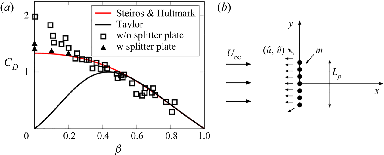
The current model is based on the work of Taylor (Reference Taylor1944), in which the wake is assumed to be described by potential flow theory at the initial expansion region near the plate. The porous plate is then represented by a distribution of sources of strength  $m$ and width
 $L_p$ (see figure 1). The sources induce the streamwise and crosswise velocities
 \begin{equation} \hat{u} = \frac{m}{2{\rm \pi}} \left( \arctan{\frac{y+L_p/2}{x}} - \arctan{\frac{y-L_p/2}{x}} \right) \end{equation}
and
 \begin{equation} \hat{v} = \frac{m}{4{\rm \pi}} \left( \ln{\frac{(y+L_p/2)^2 + x^2}{(y-L_p/2)^2 + x^2}} \right), \end{equation}
respectively. The flow velocity may then be computed by superposing the above velocities to the unperturbed flow  $\boldsymbol {U} = (U_0,0 )$ which, for this flow case, is equal to the free-stream velocity
 $U_\infty$. Using this flow representation, Taylor (Reference Taylor1944) obtained the following prediction for the drag coefficient of an unconfined porous plate:
 \begin{equation} C_D = 4 u^* (1-u^*), \end{equation}
where  $u^* = u/U_\infty$, with
 $u$ being the velocity through the porous plate. The above prediction is identical to the one obtained using the Rankine–Froude theory (Hansen Reference Hansen2015), which constitutes the basis of most blockage correction models for porous plates and wind turbines. Figure 1 shows the well-known failure of the Rankine–Froude–Taylor theory when porosity becomes small, which limits the applicability of blockage correction models to high-porosity regimes (Apelt & West Reference Apelt and West1975; Ross & Polagye Reference Ross and Polagye2020a; Miller et al. Reference Miller, Duvvuri and Hultmark2021). Appendix A presents a relation that connects
 $u^*$ with
 $\beta =A_p/A$ (where
 $A_p$ and
 $A$ are the porous and gross areas of the plate, respectively), proposed by Taylor & Davies (Reference Taylor and Davies1944).
(a) Comparison of the predictions of Taylor (Reference Taylor1944) and Steiros & Hultmark (Reference Steiros and Hultmark2018) with drag measurements of plates of varying porosity  $\beta$. In certain low-porosity cases, a splitter plate is used to suppress vortex shedding. Data are taken from Steiros & Hultmark (Reference Steiros and Hultmark2018). (b) Superposition of a distribution of sources of strength
 $m$ on a free stream, corresponding to the Taylor model.

The above limitation can be corrected by refining the Taylor model so that (i) continuity is imposed across the plate (Koo & James Reference Koo and James1973), and (ii) the wake pressure can assume lower than ambient values, which are calculated implicitly using momentum theory (Steiros & Hultmark Reference Steiros and Hultmark2018). This representation then yields the revised prediction
 \begin{equation} C_D = \frac{4}{3}\,\frac{(1-u^*)(2+u^*)}{2-u^*}, \end{equation}
which, as shown in figure 1, is in much better agreement with experimental data for small plate porosities, as long as vortex shedding is absent or suppressed via the use of a splitter plate. A blockage correction model based on the refined theory of Steiros & Hultmark (Reference Steiros and Hultmark2018) could thus offer increased accuracy in high-solidity regimes.
2.2. Confined plate kinematics
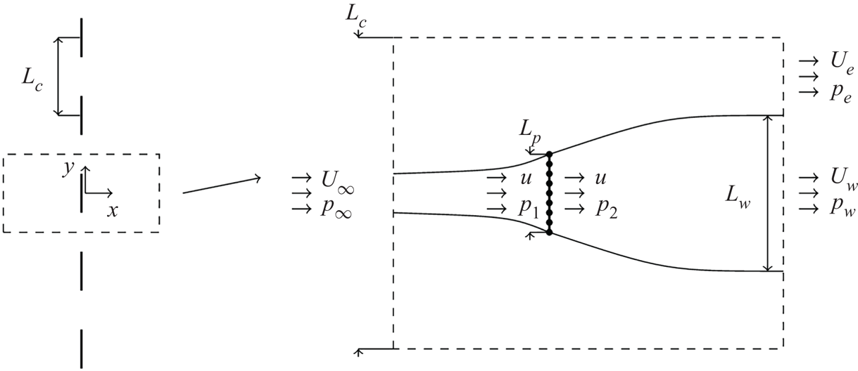
Following Koo & James (Reference Koo and James1973), the effect of channel walls in the above flow representation is introduced via the method of mirror images. An infinite number of plates are positioned side by side, with the distance between their centres being equal to the channel width  $L_c$ (see figure 2). The induced velocities from each plate are then
 \begin{equation} \hat{u}_n = \frac{m}{2{\rm \pi}} \left( \arctan{\frac{y+L_p/2-n L_c}{x}} - \arctan{\frac{y-L_p/2-n L_c}{x}} \right) \end{equation}
and
 \begin{equation} \hat{v}_n = \frac{m}{4{\rm \pi}} \left( \ln{\frac{(y+L_p/2 -n L_c)^2 + x^2}{(y-L_p/2 -n L_c )^2 + x^2}} \right), \end{equation}
where  $n \in \{\ldots, -2, -1, 0, 1, 2,\ldots \}$ and
 $n=0$ is the original plate. To calculate the velocity of the fluid, we need to sum the contribution of all plates, and on top of that add the unperturbed velocity of the stream if no plates were present,
 $(U_0,0)$.
Schematic of the flow model. An infinite number of plates, positioned side by side at a distance  $L_c$, represent the flow around a porous plate inside a channel.

It can be checked readily that the addition of the image plates does not alter the axial velocity through the plate  $u$, which retains its unconfined value (see Steiros & Hultmark Reference Steiros and Hultmark2018):
 \begin{equation} u = U_0 - \frac{m}{2}. \end{equation}
Far upstream or downstream from the plate, however, the induced velocities of the images add up to a non-negligible axial velocity contribution. In particular, the velocity at the centreline  $y=0$ becomes
 \begin{equation} u_{x \rightarrow \pm\infty} = U_0 \pm \lim_{x\rightarrow \pm\infty}{ \sum_{n={-}\infty}^{\infty} \hat{u}_n (x,0 )}, \end{equation}
where the minus corresponds to upstream, and plus to downstream. For large distances from the plate  $|x|$, we have
 $|\hat {u}_{n+1} (x,0 ) - \hat {u}_{n} (x,0 ) | \ll |\hat {u}_{n} (x,0 )|$, and thus
 $\sum _{n=-\infty }^{\infty } \hat {u}_n (x,0 )$ can to a good approximation be considered a continuous function of the continuous variable
 $\tilde {n}$. The series can therefore be replaced by an integral, i.e. (note that (2.7) is also used)
 \begin{equation} u_{x \rightarrow \pm \infty} = U_0 \pm \lim_{x\rightarrow \pm \infty}{ \int_{-\infty}^{\infty} \hat{u}_{\tilde{n}} (x,0 ) \,{\rm d} \tilde{n} } = U_0 \pm (U_0-u) b, \end{equation}
where  $b = {L_p}/{L_c}$. This yields an expression for the free-stream velocity in the channel
 $U_\infty = u_{x \rightarrow - \infty }$, i.e.
 \begin{equation} \frac{U_\infty}{U_0} = 1 - \left(1-\frac{u}{U_0} \right)b = \frac{1-b}{1-u^*b}, \end{equation}
where  $u^* = u/U_\infty$. Expression (2.10) shows that the free-stream velocity depends on the level of blockage. For instance, when a plate is fully blocking the channel (
 $b=1$), the free-stream velocity will be equal to the velocity through the plate, i.e.
 $U_\infty = u$, even if the ‘nominal’ channel velocity
 $U_0$ is larger than that.
The wake velocity can be obtained from  $u_{x \rightarrow \infty }$ after applying a correction to it. In particular, as Koo & James (Reference Koo and James1973) first noted, the source representation produces a discontinuity at the plate location
 $(x,y)=(0,0)$, as the velocity immediately upstream of the plate
 $u^{-}=U_0 - m/2$ is different to the velocity immediately downstream of the plate
 $u^{+}=U_0 + m/2$, violating the conservation of mass and momentum. To impose continuity across the plate, Koo & James (Reference Koo and James1973) proposed a rescaling of the velocities of the whole wake by a factor
 $E = u^{-}/u^{+}$. Using (2.7) and (2.10),
 $E$ becomes in our case
 \begin{equation} E = \frac{U_0 - m/2}{U_0 + m/2} = \frac{u^*}{2U_0/U_\infty-u^*} = \frac{u^*(1-b)}{2 - u^* - u^*b} , \end{equation}
and thus the far wake velocity after the rescaling becomes
 \begin{equation} \frac{U_w}{U_\infty} = \frac{Eu_{x \rightarrow \infty} }{U_\infty} = E \left ( \frac{U_0}{U_\infty} + \left(\frac{U_0}{U_\infty} - u^* \right) b \right) = \frac{u^*(1-2 u^*b +b)}{2 - u^* - u^*b} . \end{equation}
This equation shows that by increasing the tunnel blockage  $b=L_p/L_c$ (i.e. by narrowing the channel), the wake velocities are also increased. Then conservation of mass dictates that the wake would be squeezed, as expected.
Finally, we consider the square crosswise velocity  $v_1^2$ at the neighbourhood of the plate, i.e. at
 $x\to 0$. This varies along
 $y$, but for simplicity we consider it constant, and equal to its average value
 $\overline {v_1^2}$. Appendix B shows that the latter can be approximated by
 \begin{equation} \overline{v_1^2} \approx \frac{(U_\infty-u)^2}{3}. \end{equation}
2.3. Conservation laws
Given the above description of the flow kinematics, we may apply conservation of mass, momentum and energy in the control volume shown in figure 2 to calculate the drag and wake pressure coefficients of the confined plate, given the normalised velocity through the plate  $u^*=u/U_\infty$ and the blockage ratio
 $b=L_p/L_c$. Conservation of mass within the wake and channel regions yields
 \begin{gather} L_p u = L_w U_w , \end{gather}
 \begin{gather}L_c U_\infty = L_w U_w + U_e (L_c-L_w ) . \end{gather}
Conservation of momentum in the channel yields
 \begin{equation} D - p_\infty L_c + p_w L_w + p_e (L_c - L_w ) = \rho L_c U_\infty^2 - \rho L_w U_w^2 - \rho (L_c - L_w ) U_e^2 , \end{equation}
where  $D= (p_1-p_2 ) L_p$ is the drag per unit length. We note that after the end of the control volume, turbulent stresses are assumed to emerge, balancing the vertical pressure gradient (see Tennekes & Lumley Reference Tennekes and Lumley1972). In the inviscid control volume, on the other hand, turbulent stresses are neglected, even though in reality they will exist in small magnitudes. We may thus expect a slight imbalance of the pressure gradient in the crosswise momentum equation.
Applying Bernoulli's equation upstream, downstream and around the plate, we obtain
 \begin{gather} p_\infty + 0.5\rho U_\infty^2 = p_1 + 0.5\rho (u^2+v_1^2 ) , \end{gather}
 \begin{gather}p_2 + 0.5\rho (u^2 + v_2^2 ) = p_w + 0.5\rho U_w^2 , \end{gather}
 \begin{gather}p_\infty + 0.5\rho U_\infty^2 = p_e + 0.5\rho U_e^2 , \end{gather}
where  $v_1^2$ is given by (2.13),
 $v_2=E v_1$, and
 $U_w$ comes from (2.12). By solving the system (2.14)–(2.19), the following analytical expressions of the flow quantities of interest can be derived, given as functions of
 $u^*$ and
 $b$:
 \begin{gather} C_D = \frac{4 (u^*b-1)(1-u^*)}{(1-b)(2-u^*-u^*b)} \left( \frac{1-u^*}{3} - \frac{1-2u^*b+b}{1-b}\right), \end{gather}
 \begin{gather}u_e^* = \frac{U_e}{U_\infty} = \frac{ 1-2u^*b + b }{1 - b}, \end{gather}
 \begin{gather}\frac{L_w}{L_c} = \frac{\left(2-u^* - u^*b \right)b}{1-2u^*b + b}, \end{gather}
 \begin{gather}Cp_w ={-} C_D + \frac{4 (1-u^*)(u^*b-1)}{(2-u^*-u^*b)^2} \left( \frac{(1-u^*)^2}{3} - (1-u^{*2}b)\right), \end{gather}
which reduce to the unconfined plate expressions of Steiros & Hultmark (Reference Steiros and Hultmark2018) for  $b=0$.
2.4. Blockage correction method
The above theoretical framework can be used to convert the flow quantities from one level of blockage (i.e. experimental conditions) to another (typically unconfined conditions). Similar to most existing blockage correction models (see e.g. Barnsley & Wellicome Reference Barnsley and Wellicome1990; Mikkelsen & Sørensen Reference Mikkelsen and Sørensen2002; Houlsby et al. Reference Houlsby, Draper and Oldfield2008; Werle Reference Werle2010), we achieve that following the rationale of Glauert (Reference Glauert1935), i.e. we seek the ‘corrected’ free-stream velocity  $U_\infty ^c$ that would produce the same values of thrust
 $T$, through-velocity
 $u$, and angular velocity
 $\omega$ (if turbines are considered) of the blocked model, but in unconfined conditions, i.e.
 \begin{equation} T^c = T^m,\quad u^c = u^m,\quad \omega^c = \omega^m, \end{equation}
where the superscripts  $c$ and
 $m$ denote corrected/unconfined data and measured/confined data, respectively. Using the actuator disk relation for power
 $P= T u$, the above also yield
 $P^c=P^m$. Expressed in non-dimensional form, the correction model consists of a set of expressions for the ‘corrected’ flow quantities as functions of the confined flow data and the free-stream velocity ratio
 $R_V={U_\infty ^m}/{U_\infty ^c}$:
 \begin{gather} \lambda^{c} = \lambda^{m} R_V , \end{gather}
 \begin{gather}C_T^c = C_T^m R_V^2 , \end{gather}
 \begin{gather}C_P^c = C_P^m R_V^3 , \end{gather}
where  $\lambda = \omega R/U_\infty$ is the turbine tip speed ratio,
 $R$ is the turbine radius, and
 $C_T = 2T/(\rho U_\infty ^2 {\rm \pi}R^2)$,
 $C_P = 2P/(\rho U_\infty ^3 {\rm \pi}R^2)$ are the turbine thrust and power coefficients, respectively. The blockage correction thus rests on the determination of the free-stream velocity ratio
 $R_V$. The latter is calculated using potential flow theory, i.e. the Rankine–Froude theory in existing models, and the framework of §§ 2.2 and 2.3 in the current work. The necessary inputs are the blockage ratio and one confined flow property, typically the thrust/drag coefficient, even though other quantities can also be used (e.g. flow-through velocity, wake width). Summarising, the blockage correction process rests on the calculation of
 $R_V = {U_\infty ^m}/{U_\infty ^c} = u^{*,c}/u^{*,m}$ and consists of the following steps.
1. Given the measured thrust coefficient
 $C_T^m$ and blockage ratio $b_m$, solve (2.20) to obtain $u^{*,m}$.
2. Solve (2.26) for
$u^{*,c}$, where $C_T^c$ is given by (2.20) and $b=b_c$ is the target blockage ratio (typically zero).3. Compute the free-stream velocity ratio
$R_V = u^{*,c}/u^{*,m}$.4. Compute the ‘blockage-corrected’ rotor/plate performance using (2.25)–(2.27).


The above described blockage correction method is expected to work for two-dimensional plates (strips) of arbitrary porosity, as long as vortex shedding is suppressed or absent. When considering turbines, the additional complexity of three-dimensionality appears, i.e. horizontal axis turbines are circular, while vertical axis turbines have a finite aspect ratio. Therefore, the current blockage model can be thought strictly appropriate for correcting rows of closely spaced turbines (Draper et al. Reference Draper, Nishino, Adcock and Taylor2016). However, in § 4.3 we show that the current model produces accurate corrections for the thrust and power of single horizontal axis wind turbines of any porosity, while it yields results almost identical to those from conventional correction models at high effective porosities, despite the conceptual differences of two- and three-dimensional flows.
3. Validation methodology
3.1. Experimental set-up
To validate the predictions of (2.20)–(2.22), experiments were carried out in the aerodynamics flume of the Aeronautics Department at Imperial College London. The facility has a test section that is  $L_c=0.6$ m wide with variable water height, which can achieve flow speed up to
 $0.8$ m s
 $^{-1}$, with free-stream turbulence intensities below 1.5 % (Cicolin et al. Reference Cicolin, Buxton, Assi and Bearman2021). The experiments were performed at the speed range from 0.2 to 0.5 m s
 $^{-1}$, leading to a variation in the Reynolds number based on the plate width,
 $Re = U_\infty L_p / \nu$, between
 $9 \times 10^3$ and
 $5.5 \times 10^4$; all porosity/blockage combinations (see below) were tested at two different Reynolds numbers (different by a factor of
 $\simeq 1.5\unicode{x2013}1.7$). The variation in the measured quantities was found to be negligible.
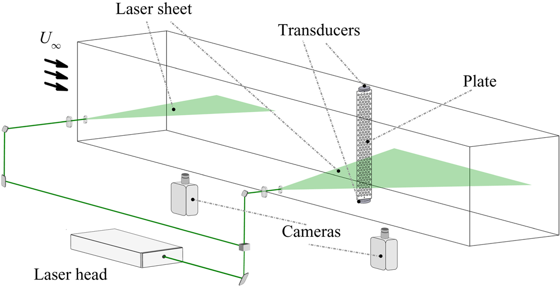
Force measurements were made using two force transducers (see figure 3), one attached to the bottom of the plates (i.e. submerged in the water), and the other attached to the top of the plates (outside the water). Each transducer (model ATI Mini 40) measures forces up to 80 N with resolution 0.005 N. The sum of the values from the two transducers yielded the total drag  $D$ acting on the plate. The drag coefficient was then calculated as
 $C_D = 2D/(\rho U_\infty ^2 A)$, with
 $A$ the gross wetted area of the plate (i.e. without subtracting the perforations). Particle image velocimetry (PIV) measurements were acquired at two different positions. The illumination source was a high-speed Litron LDY 304 Nd:YLF laser, which operated at constant frequency 1 kHz. An optical system split the laser beam into two components. One illuminated a small field of view upstream, intended to measure the incoming flow speed, while the second laser sheet illuminated the wake of the plate, as illustrated in figure 3. The images were captured and recorded by two cameras, model Phantom v641, with a maximum resolution
 $2460\times 1600$ px and internal storage memory for 5700 images at the highest resolution. The laser pulse and each camera operated at different acquisition rates, and their synchronisation was performed through an external pulse generator (Stanford DG645).
Schematic of the experimental apparatus and measurement techniques.

In total, 16 plates of 5 mm thickness aluminum were tested, where circular holes were water jetted leading to porosity ratios  $\beta$ of 0 %, 15 %, 30 % and
 $50\,\%$. The plates spanned the whole height of the flume (with the exception of a small area underneath the plates where the force sensor was positioned). Each porosity ratio was applied to four different plate widths
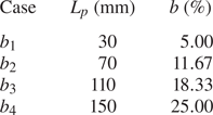
 $L_p$, leading to four blockage ratios for each porosity case (see table 1). For the
 $\beta$ cases of
 $0\,\%$ and
 $15\,\%$, a 450 mm long splitter plate was positioned in the wake of the plates, in order to suppress vortex shedding, which otherwise appears in low porosities (Steiros, Bempedelis & Ding Reference Steiros, Bempedelis and Ding2021). Acquisition started after the flow was stabilised, typically after two minutes from the moment the flume speed was set up. Force and PIV measurements were acquired simultaneously. The forces were acquired at constant frequency 100 Hz, whereas the PIV acquisition varied from 4 to 20 Hz, depending on the temporal scale of the model. The acquisition period was chosen to be sufficient to obtain at least 100 cycles of vortex shedding, considering the reference case of the solid plate. The field of view was constant in all experiments, covering an area
 $340\times 210$ mm
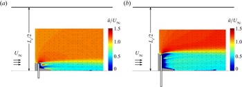
 $^2$, as shown in figure 4. The wake width
 $L_w$ was calculated as the maximum distance from the centreline reached by the streamline of the mean flow starting from the tip of the plate. The velocity between the channel wall and the wake border
 $U_e$ was calculated as the asymptotic value of the streamwise velocity away from the plate.
Details of experimental configurations. Channel width is  $L_c=600$ mm,
 $L_p$ is the plate width, and
 $b=L_p/L_c$ is the blockage ratio.

Mean velocity fields for two plates of  $\beta =50\,\%$ at different blockage ratios obtained using PIV: (a)
 $b=11.67\,\%$, (b)
 $b=25\,\%$.

3.2. Numerical simulations
Large-eddy simulations (LES) of the flow around model wind turbines were performed using Xcompact3d, a finite-difference framework that uses sixth-order compact schemes to solve the incompressible Navier–Stokes equations (Laizet & Lamballais Reference Laizet and Lamballais2009; Laizet & Li Reference Laizet and Li2011; Bartholomew et al. Reference Bartholomew, Deskos, Frantz, Schuch, Lamballais and Laizet2020; Deskos, Laizet & Palacios Reference Deskos, Laizet and Palacios2020). In the present work, the wind turbines were modelled by the actuator line method, the standard Smagorinsky model was used to model the effects of the unresolved fluid motions, and a third-order Adams–Bashforth method was used for time integration.
The considered configurations were based loosely on the experiments of the ‘Blind Test 1’ (BT1) workshop (Krogstad & Eriksen Reference Krogstad and Eriksen2013). Xcompact3d has been used previously to study this particular problem, showing very good agreement with the experimental results (Deskos, Laizet & Piggott Reference Deskos, Laizet and Piggott2019; Bempedelis & Steiros Reference Bempedelis and Steiros2022). In this work, we considered the high-solidity six-bladed variant of the BT1 turbine. Two square channels, a small one of two turbine diameters width, and a large one of five diameters width, allowed the simulation of blockage ratios of  $\simeq 19.6\,\%$ and
 $\simeq 3.1\,\%$, respectively. The turbines were positioned at the centre of the square channel, creating close to isotropic blockage. The channel length in both cases was 12 turbine diameters. Slip conditions were used at the lateral domain boundaries, and laminar inflow (
 $U_\infty =10$ m s
 $^{-1}$, yielding
 $Re=U_\infty D / \nu = 5.95 \times 10^5$) was considered at the inlet. (Very low turbulence levels,
 $I \simeq 0.3\,\%$, were present in the experiments; Krogstad & Eriksen Reference Krogstad and Eriksen2013.) A uniform grid consisting of 32 fluid mesh points per turbine radius was used, resulting in meshes of size
 $\simeq 13$ and
 $\simeq 79 \times 10^6$ points, respectively; such a resolution has been shown to be sufficient for the purposes of this study through comparisons with experimental data (Deskos et al. Reference Deskos, Laizet and Piggott2019; Bempedelis & Steiros Reference Bempedelis and Steiros2022). Each blade/actuator line was discretised with 52 elements, and the tower and nacelle were omitted. After an initialisation period, time series of thrust
 $T$ and power
 $P$ were extracted over
 $\simeq 64\unicode{x2013}128$ rotations, depending on the angular velocity of the turbine
 $\omega$. The thrust and power coefficients were subsequently calculated as
 $C_T = 2T/(\rho U_\infty ^2 {\rm \pi}R^2)$ and
 $C_P = 2P/(\rho U_\infty ^3 {\rm \pi}R^2)$, respectively, with
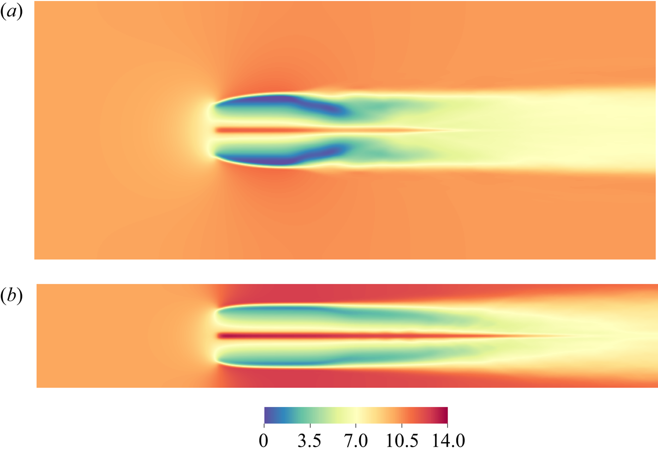
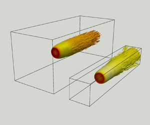
 $R$ being the turbine radius. An example view of the mean streamwise velocity of the same wind turbine in the two different channels is shown in figure 5.
Mean streamwise velocity contours at a horizontal cut through the turbine centreline,  $\lambda =6$, for two channels of different sizes: (a)
 $b=3.1\,\%$, (b)
 $b=19.6\,\%$.

4. Results
The accuracy of the proposed framework is first assessed by comparing the predictions of (2.20)–(2.22) with the experimental measurements for the porous plates, as described in § 3.1. We subsequently test the validity of the blockage correction method that builds on the theoretical model, using wind turbine data. Comparisons against existing blockage correction models are also performed.
4.1. Flow model validation
The predictions of the model for the drag coefficient  $C_D$, bypass velocity
 $u_e^* = U_e / U_\infty$ and wake size
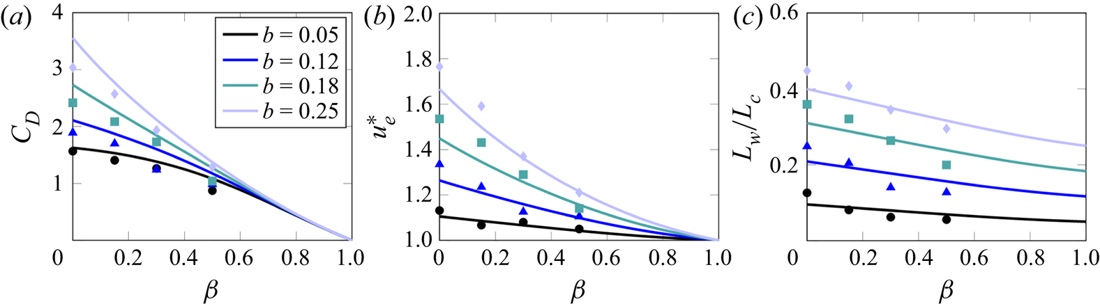
 $L_w/L_c$ at different levels of confinement (given by (2.20)–(2.22)) are shown in figure 6, where they are compared with the data measured in the porous plate experiments. The flow quantities are plotted as functions of the plate porosity
 $\beta$ instead of the normalised velocity through the plate
 $u^*$, as the latter is not easy to determine experimentally. The relation that was used to link
 $u^*$ and
 $\beta$ is given in Appendix A. The proposed model demonstrates, in general, convincing agreement with the experimental results, showing an intensification of blockage effects as porosity is decreased. It is noted, however, that there is a deterioration of the model accuracy as blockage and solidity increase. This could perhaps be attributed to the gradual emergence of viscous phenomena, which are not taken into account by the potential flow analysis. For instance, the effect of boundary layers on the flow field is not modelled by the slip condition of the method of images. This effect will be negligible when the plate is far from the channel walls (low blockage), but will increase in relevance as the blockage grows. Another possibility is the emergence of shear layer instabilities that mix the wake. Potential flow models assume that these become significant only far enough from the plate and do not directly affect the inviscid near wake. However, the increasing velocity gradients at higher blockages might cause them to appear earlier, introducing additional uncertainties.

4.2. Comparison with confined Rankine–Froude theory
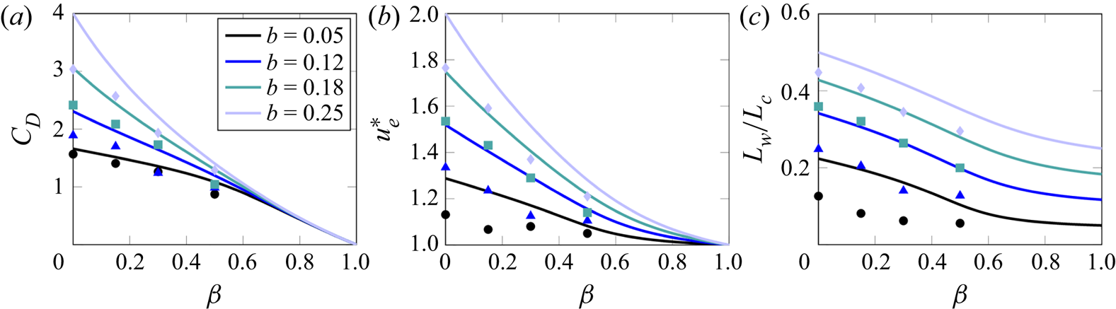
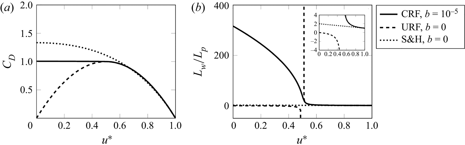
Figure 7 compares the predictions of the Rankine–Froude theory, derived for confined conditions by a number of authors (e.g. Garrett & Cummins Reference Garrett and Cummins2007), with the porous plate data. Though agreement is worse than that of the currently proposed theory (see figure 6), especially regarding the channel velocity and wake width, the confined Rankine–Froude theory captures qualitatively the trends of the experimental measurements. This result might seem a bit counter-intuitive, given the complete failure of the unconfined Rankine–Froude theory at low porosities (for instance, a solid plate is predicted to produce zero drag; see figure 1). To understand what changes with the introduction of confinement, we consider the wake width prediction of Rankine–Froude theory in unconfined conditions (Hansen Reference Hansen2015),
 \begin{equation} \frac{L_w}{L_p} = \frac{u^*}{2u^* - 1}, \end{equation}
which yields an infinite wake width at  $u^* = 0.5$ (corresponding to
 $\beta \approx 0.5$), and unrealistic wakes of negative width for smaller porosities. We note that
 $0 \leq \beta <0.5$ is the range of porosities where the unconfined drag predictions depart from observations (see figure 1). This unrealistic expansion occurs because Rankine–Froude theory assumes a strict equalisation of pressures (
 $p_w = p_\infty$) at the end of the control volume. Given that turbulent mixing is not included in the inviscid analysis, the only mechanism that enables pressure recovery is the initial expansion of the wake. As porosities decrease, the necessary expansion becomes larger, and eventually infinite at
 $u^*=0.5$.
Predictions of the confined Rankine–Froude theory for flow quantities at different levels of confinement (solid lines). Symbols show experimental measurements.

In confined conditions, on the other hand, the outer pressure  $p_e$ is not fixed to
 $p_\infty$. Similar to the unconfined case, the wake has to expand in order for
 $p_w$ to become equal to
 $p_e$. As a result, the outer flow is squeezed, leading to an increase in
 $u_e$ and a decrease in
 $p_e$. Therefore,
 $L_w$ will tend to approach the channel (driven by the unrealistic wake expansion) but will never reach it, because the limit
 $L_w \to L_c$ would lead to
 $p_e \to - \infty$, and the wake pressure will be equalised with
 $p_e$ before that happens. It is perhaps instructive to consider the limit
 $b \to 0$ (but not exactly zero), shown in figure 8. (Note that the confined Rankine–Froude theory may admit multiple solutions; here, we choose the most realistic one, i.e. the one yielding positive wake sizes.) In that case,
 $L_w$ will assume unrealistically large values at
 $u^*=0.5$, as in the unconfined case (see (4.1)). For lower
 $u^*$, however, the wake size will not become negative, as in the unconfined case, but will continue to tend to infinity. As a result, the predicted drag will reach
 $C_D=1$ at
 $u^* = 0.5$, as in the unconfined case, and will then plateau at that value for lower porosities. It may then be concluded that, despite giving the impression of correct modelling, at least for the drag, the imposition of channel walls may result in a behaviour that is equally unphysical compared to the unconfined case.
Predictions of the confined Rankine–Froude theory (CRF) for  $\beta \to 0$, the unconfined Rankine–Froude theory (URF), and the Steiros & Hultmark (Reference Steiros and Hultmark2018) (S&H) theory for (a) drag and (b) wake size. Also shown is a zoomed-in plot of the wake size.

A more physical approach is to assume that the eventual pressure recovery will be partly due to the initial wake expansion, and partly due to turbulent mixing, the latter assumed to occur after the end of the inviscid control volume. The assumption  $p_w=p_\infty$ is thus relaxed to
 $p_w$ assuming arbitrary values, which have to be determined using additional information (e.g. experimental data (Roshko Reference Roshko1954), or the source description in the current work). Such treatment is known to considerably improve the model predictions (see figure 1), and has been employed in numerous studies (see, for instance, Yeung & Parkinson (Reference Yeung and Parkinson2000) and references therein), including the current paper. A purely inviscid pressure recovery can be considered a valid approximation only for highly porous plates, where the pressure is only minimally perturbed and turbulent mixing is negligible. In that case, the Rankine–Froude theory indeed produces reliable and consistent results.
4.3. Blockage correction
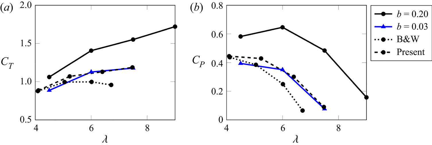
Having validated the flow model, we proceed to assess the accuracy of the blockage correction method that builds on it. Figure 9 plots the thrust and power coefficients of the simulated high-solidity turbines presented in § 3.2 as functions of the tip speed ratio  $\lambda = \omega R/U_\infty$. As expected, a smaller computational domain contributes to significantly larger thrust and power, underlining the need for blockage corrections. The corrections of the present method (i.e. § 2.4) and from Barnsley & Wellicome (Reference Barnsley and Wellicome1990) (described in Ross & Polagye Reference Ross and Polagye2020a) are also plotted in figure 9. Note that the method of Barnsley & Wellicome (Reference Barnsley and Wellicome1990) is similar to that described in Bahaj et al. (Reference Bahaj, Molland, Chaplin and Batten2007), and was among the best-performing ones in Ross & Polagye (Reference Ross and Polagye2020a). The two methods produce comparable results that agree with the negligible blockage simulation data at low tip speed ratios, as the induction factor (and thus the effective solidity of a turbine) is expected to be analogous to
 $\lambda$. However, as the latter increases, the method of Barnsley & Wellicome (Reference Barnsley and Wellicome1990) becomes increasingly more inaccurate compared with the current method, due to the failure of the Rankine–Froude theory at high solidities.
Application of the corrections by Barnsley & Wellicome (Reference Barnsley and Wellicome1990) (B&W) and the present model to the simulated high induction factor (i.e. solidity) wind turbines.

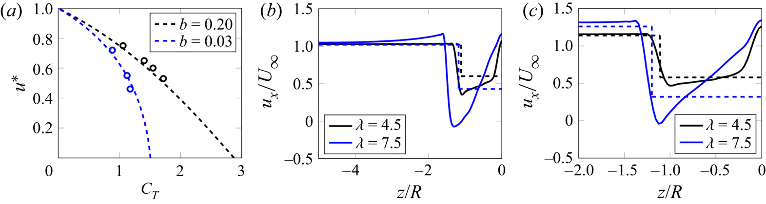
Figure 10 provides an inspection of the changes in the velocity field induced by the increase in blockage. First, we plot the relation between the velocity through the rotor  $u^*$ and the thrust coefficient for the simulated turbines. The calculation of
 $u^*$ was performed by integrating the mean streamwise velocity immediately upstream of the turbine rotor. The model predictions are in good agreement with the turbine data at both low and high blockage conditions. However,
 $u^*$ is an integrated quantity, and as seen in figure 5, the velocity can vary along the turbine radius. Figure 10 also shows the numerically predicted near wake velocity profiles in the two channels, along a horizontal cut (i.e. along the
 $z$ direction) from the turbine centreline to the domain edge. The profiles are extracted at a location where the streamlines passing from the rotor tip achieve their maximum width. Also plotted are the predictions of the model, which assumes a top hat profile for all quantities. The model captures qualitatively the wake deficit, size and channel velocity, as well as their trends with increasing blockage and induction factor. However, similar to the plate data, it underestimates the channel velocities as blockage increases. The top hat assumption of the model is shown to be more relevant for small induction factors, as strong gradients appear at higher induction factors. However, these gradients are to a large degree manifest in the simulations due to the omission of the nacelle (see § 3.2), which leads to the formation of a high-speed jet at the centre of the turbine, which would not appear in realistic configurations.
(a) Rotor through velocity  $u^*$ versus thrust coefficient. Streamwise velocity
 $u_x$ profiles at different blockage levels: (b)
 $b=0.03$, (c)
 $b=0.20$. Model predictions are shown by dashed lines, numerical simulations by symbols and solid lines.

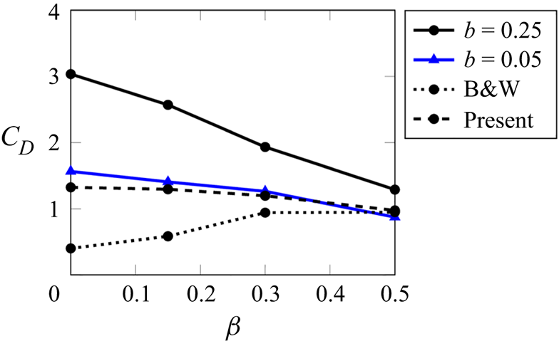
Figure 10 shows that the smallest simulated  $u^*$ was approximately 0.46, i.e. the turbine operates in a regime where the predictions of the Rankine–Froude theory for the thrust are not significantly inaccurate (see figure 8). In higher solidity regimes, the departure of classical blockage models is expected to be larger. This is verified by applying the two corrective methods to the porous plate data for the highest tested blockage ratio,
 $b=25\,\%$ (see figure 11). The predictions of the proposed correction display good agreement with the ‘near-unconfined’ data,
 $b=5\,\%$. On the other hand, the deviation in the predictions of the Barnsley & Wellicome (Reference Barnsley and Wellicome1990) correction becomes quite significant as porosity (and thus
 $u^*$) tends to zero.
Predictions of the blockage correction model (dashed line) against experimental measurements (solid lines). Also shown is the correction of the Barnsley & Wellicome (Reference Barnsley and Wellicome1990) model (dotted line).

The above results suggest that the present model is indeed appropriate for correcting blockage effects in high-solidity turbines and plates. A natural question is then: how does the current model fare in low-solidity wind turbine regimes, where conventional models are still accurate? To answer that, we use the publicly available experimental data of Ross & Polagye (Reference Ross and Polagye2020a), who tested the performance of low-induction turbines at two facilities of different sizes (under high blockage,  $b=35\,\%$, and negligible blockage,
 $b=2\,\%$). The reader is referred to Ross & Polagye (Reference Ross and Polagye2020a) for details of the experimental configurations.
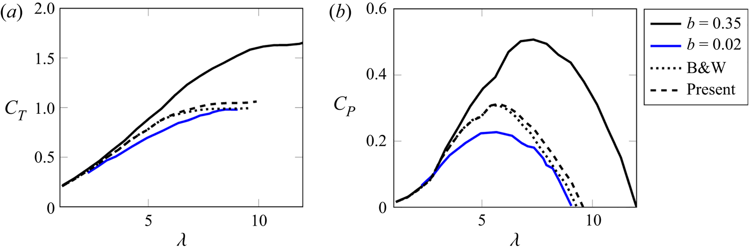
Figure 12 compares the results of the proposed theory with the axial flow turbine data of Ross & Polagye (Reference Ross and Polagye2020a), as well as with the predictions of the method of Barnsley & Wellicome (Reference Barnsley and Wellicome1990) (also extracted from Ross & Polagye Reference Ross and Polagye2020a). The two methods produce almost identical predictions for both thrust and power coefficients, showing that potentially, the current model can replace standard ones at any induction factor. It is noteworthy to mention that at high tip speed ratios ( $\lambda >7$), the current model predicts unconfined thrust coefficients that exceed unity, departing slightly from the method of Barnsley & Wellicome (Reference Barnsley and Wellicome1990), which plateaus at unity as soon as it reaches this value. The latter behaviour is problematic, and reflects the limitations of the Rankine–Froude–Taylor theory, where drag coefficients may not exceed unity.
Application of the corrections by Barnsley & Wellicome (Reference Barnsley and Wellicome1990) and the present model to the low induction factor (i.e. solidity) axial flow turbine data of Ross & Polagye (Reference Ross and Polagye2020a). Both corrective models show comparable accuracy.

5. Summary and conclusions
By combining the potential flow representation of Steiros & Hultmark (Reference Steiros and Hultmark2018) for porous plates with the method of images to simulate channel walls, a novel blockage correction model for wind turbines and porous plates of arbitrary solidity/induction factor was developed. The steps of the correction algorithm are presented in § 2. High fidelity laboratory and numerical experiments with porous plates and wind turbines indicated that the proposed correction performs equally as well as conventional ones in low-solidity regimes, but becomes more accurate as the solidity/induction factor increases. The applicability of the current model might be somewhat limited in conventional horizontal axis wind turbines, as they tend to operate in low-solidity regimes, but might become especially relevant when considering blockage effects in high-solidity configurations such as many-bladed vertical axis wind turbines, tidal turbines, and more generally bluff bodies of arbitrary porosity, including the fully solid limit in which splitter plates are used to suppress vortex shedding, and where no blockage correction model is currently available (see, for instance, Apelt & West Reference Apelt and West1975; Chapman et al. Reference Chapman, Masters, Togneri and Orme2013; Miller et al. Reference Miller, Duvvuri and Hultmark2021).
Acknowledgements
The authors would like to thank Mr Edward O'Brien for his help with preliminary numerical simulations.
Funding
K.S. was supported by Imperial College London via a Junior Research Fellowship. N.B. was supported by EPSRC, grant no. EP/V000942/1.
Declaration of interests
The authors report no conflict of interest.
Appendix A. Connection between $u^*$ and $\beta$


The current theoretical framework uses the variable  $u^*=u/U_\infty$ as its input. However, in many cases, the latter is difficult to measure, and it is more convenient to express all quantities as functions of the porosity ratio
 $\beta$. To connect the two, Taylor & Davies (Reference Taylor and Davies1944) proposed the following expression when friction losses are negligible:
 \begin{equation} C_D \approx u^{*2}\left(\frac{1}{\beta^2}-1\right). \end{equation}
The main assumptions behind this expression are that the surplus kinetic energy, due to acceleration of the fluid that enters the plate pores, becomes heat irreversibly, and that the effect of the vena contracta is negligible. Taylor & Davies (Reference Taylor and Davies1944) provide experimental validation for the above formula (see Steiros & Hultmark (Reference Steiros and Hultmark2018) for a reproduction of their validation plot). This formula has been used repeatedly in previous works (see, for instance, Castro Reference Castro1971; Graham Reference Graham1976). Combination of the above equation with (2.20) yields an expression linking  $\beta$ and
 $u^*$.
Appendix B. Crosswise velocity at the vicinity of the plate
Using the method of images described in § 2.2, we obtain the following crosswise velocity for  $x\to 0$:
 \begin{equation} v_1 = \frac{m}{4 {\rm \pi}} \sum_{n={-}\infty}^{+\infty} \left[ \ln \left( \frac{y' + 1 - n/b}{y' - n/b} \right) \right], \end{equation}
where  $y'=y/L_p - 1/2$. At the unconfined limit,
 $b\to 0$, the above yields the unconfined plate velocity (2.2), whose average square value, as shown in Steiros & Hultmark (Reference Steiros and Hultmark2018), is
 \begin{equation} \overline{v_1^2} = m^2/12 = (U_0 - u)^2/3 = (U_\infty - u)^2/3 . \end{equation}
In the above, we have used (2.7) and the fact that at  $b=0$,
 $U_\infty = U_0$ from (2.10). On the other hand, at the fully confined limit,
 $b=1$, the velocity
 $v_1$ becomes
 \begin{equation} v_1 = \frac{m}{4 {\rm \pi}} \ln \frac{\displaystyle\prod_{n={-}\infty}^{+\infty} (y' + 1 - n )}{\displaystyle\prod_{n={-}\infty}^{+\infty} (y' - n)} = 0 , \end{equation}
i.e. if the plate spans the channel fully, then there cannot be any crosswise velocity. In that case as well, then, the average square crosswise velocity is
 \begin{equation} \overline{v_1^2} = 0 = (U_\infty - u)^2/3 , \end{equation}
where we used the fact that  $U_\infty = u$ when
 $b=1$ (see (2.10)). Given the above, we use the approximation
 $\overline {v_1^2} \approx (U_\infty - u)^2/3$ for any level of blockage
 $0 \leq b \leq 1$. This expression is strictly valid only at the two limits
 $b=0$ and
 $b=1$, while it can be shown readily that it expresses a linear approximation of the velocity
 $v_1$ for the in-between blockage values, i.e.
 $v_1^{conf} \approx v_1^{unc} (1-b)$, where
 $v_1^{conf}$ and
 $v_1^{unc}$ are the confined and unconfined crosswise velocities at the vicinity of the plate, respectively.