1 Introduction
The transition of the shear layers which form on bluff bodies is an essential subject in fluid mechanics. The mechanisms which govern shear layer transition are comparable to plane mixing layers and include the amplification of disturbances, the formation of Kelvin–Helmholtz (KH) vortices and vortex pairing. These phenomena are a profound exhibition of the evolving dynamic behaviour of fluids. For bluff-body flow, a distinguishing feature is that shear layer transition takes place as a part of an extended flow field and therefore is considerably more complex than the two-dimensional mixing layer. Nonetheless, substantial attention has been directed towards documenting the characteristics of bluff-body shear layer transition; however, within the literature, virtually all endeavours are concerned with the circular cylinder (‘cylinder’) (Bloor Reference Bloor1964; Prasad & Williamson Reference Prasad and Williamson1997; Rajagopalan & Antonia Reference Rajagopalan and Antonia2005). A hallmark of these studies is the consideration of the nonlinear scaling of the KH instability frequency,
 $f_{KH}$
, normalised by the von Kármán (VK) frequency,
 $f_{VK}$
, with Reynolds number,
 $Re_{D}=U_{\infty }D/\unicode[STIX]{x1D708}$
, where
 $D$
is the body diameter and
 $U_{\infty }$
is the free-stream velocity. The debate over the detail of the power-law dependence of
 $f_{KH}/f_{VK}$
on
 $Re_{D}$
and the physical defence of its origin is now more than a half-century old and remains ongoing. In spite of these undertakings, there are only a few investigations to have probed the nature of shear layer transitioning from sharp-edged bluff bodies, such as a square prism (‘prism’). Indeed, there are presently no studies that have systematically reported the shear layer frequencies for the prism over a broad range of
 $Re_{D}$
. This study seeks to furnish the literature with some measurements and analysis in response to this need.
For the cylinder, Bloor (Reference Bloor1964) first proposed a power-law scaling by dimensional considerations. That is, the shear layer frequency is proportional to a velocity scale over a length scale. A frequency ratio scaling argument for the bluff-body shear layer was therefore
 $$\begin{eqnarray}\displaystyle \frac{f_{KH}}{f_{VK}}\propto \frac{U_{KH}}{L_{KH}}\frac{L_{VK}}{U_{VK}}. & & \displaystyle\end{eqnarray}$$
According to Bloor,
 $L_{VK}=D$
while both
 $U_{KH}=U_{VK}=U_{\infty }$
. The length
 $L_{KH}$
was the boundary layer thickness at separation, which was dependent on the free-stream velocity according to
 $\unicode[STIX]{x1D6FF}_{sep}\propto 1/U_{\infty }^{1/2}$
. Thus only
 $L_{KH}$
exhibited nonlinear behaviour and her final argument was
 $$\begin{eqnarray}\displaystyle \frac{f_{KH}}{f_{VK}}\propto Re_{D}^{1/2}. & & \displaystyle\end{eqnarray}$$
Prasad & Williamson (Reference Prasad and Williamson1997) contended for an exponent larger than
 $1/2$
because parameters unacknowledged by Bloor also exhibit
 $Re_{D}$
dependence. Their argument championed the momentum thickness at the ‘transition point’ as the appropriate length scale of the shear layer. Therefore, they introduced an
 $Re_{D}$
dependence on the shear layer thickness and the distance to the point of transition. Furthermore, they also observed and acknowledged the slight influence of
 $Re_{D}$
on
 $U_{KH}=U_{sep}$
and
 $St_{D}=f_{VK}D/U_{\infty }$
. Their refined physical arguments, which captured important features of shear layer transition, produced an exponent of 0.69 in the frequency ratio scaling. This value was in good agreement with their measurements and reanalysis of the data in the literature for the cylinder.
Such considerations for the prism are absent in the literature, as are attendant measurements. Of course, the scaling argument for the prism proceeds similarly to the cylinder, as proposed by Bloor (Reference Bloor1964). Indeed, it is only a matter of identifying the significant length and velocity scales for the shear layer and the wake. However, there are compelling and significant differences for the class of bluff bodies with sharp edges, which warrant consideration. For example, the salient edges of the prism fix the separation location for all
 $Re_{D}$
and control the condition of the boundary layer at separation. As the flow accelerates around the leading edges, the surface pressure on the front face near separation asymptotically decreases. In comparison, the shear layer of the cylinder separates in the presence of an adverse pressure gradient. Sigurdson (Reference Sigurdson1986) estimated the thickness of the boundary layer on the front face of a coaxially aligned blunt-faced cylinder using the semi-empirical Thwaites method. In contrast to the circular cylinder, the front-face boundary layer exponentially thinned with increased radial distance from stagnation. Furthermore, Sigurdson (Reference Sigurdson1986) also found that the front-face boundary layer is stable up to
 $Re_{\unicode[STIX]{x1D6FF}}=(\unicode[STIX]{x1D6FF}U)_{sep}/\unicode[STIX]{x1D708}\simeq 10^{9}$
(
 $Re$
based on boundary layer thickness and velocity at separation). The prism will also have a thinning boundary layer, as the front-face pressure gradient is similar. This characteristic will impact the dynamics of shear layer transition on the prism and therefore influence features of the scaling argument.
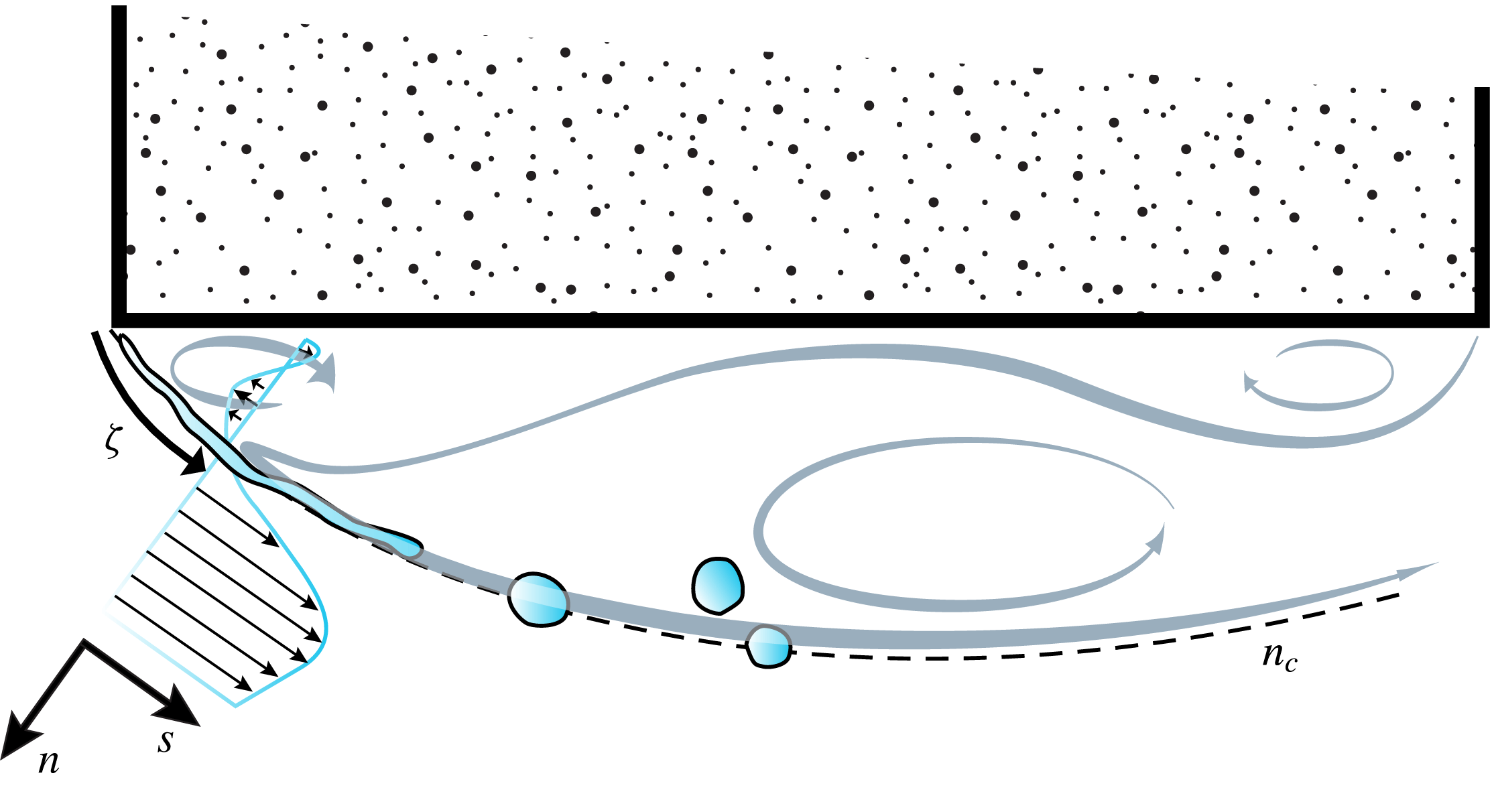
Furthermore, for a prism with no angle of incidence to the flow, beyond separation, the shear layer separates with its local axis initially perpendicular to the free stream, and therefore features a short length with high curvature, as illustrated in figure 1. It follows that the alignment between the axis of the time-averaged shear layer centre and the Cartesian coordinate system changes along its length. Therefore, one must consider the appropriate reference frame to observe the development of the prism shear layer. Mignot et al. (Reference Mignot, Vinkovic, Doppler and Riviere2014) adopted a curvilinear coordinate system referenced to the time-averaged position of a shear layer formed at a three-branch T-junction. This coordinate system aligns the velocity components orthogonal to the time-averaged streamlines. Additionally, the transformation aligns the reference frame with the highest gradients in the flow and permits observation of the local conditions leading to the KH instability.
With these considerations, this investigation seeks to observe and understand some features of the mechanisms of transition in the shear layers of a prism, explicitly considering the influences of the prism geometry. In particular, our goal is to document the evolution of the dominant shear layer instability frequency as a function of
 $Re_{D}$
and the scaling properties which buttress this frequency. In the following, § 2 presents the experimental set-up, § 3 presents results while § 4 summarises and concludes.
Schematic of the square-prism shear layer. The grey arrows are based on time-averaged streamlines to accentuate the three distinct regions of recirculation. The definition of the local coordinate system:
 $(s,n)$
are tangential and normal to the time-averaged position of the shear layer centre,
 $n_{c}$
. The arclength of the shear layer is
 $\unicode[STIX]{x1D701}$
.

2 Experimental set-up
Experiments were performed in the subsonic tunnel at the Center for Flow Physics and Control at Rensselaer Polytechnic Institute. The blow-down, open return tunnel is driven by a 100 horsepower electric motor with a centrifugal blower. A
 $9:1$
contraction with flow conditioning honeycomb and three meshes separate the settling chamber from the test section, which has a 0.8 m by 0.8 m cross-section and is 5 m long. Air density was compensated for local temperature and barometric pressure. Flow homogeneity across the middle 0.5 m of the test section was within
 $\pm 0.1$
% of the mean wind speed. The corresponding longitudinal free-stream turbulence was measured to be less than 0.3 %, decreasing slightly with increasing wind speed.
A two-dimensional square prism of
 $D=76.2$
mm and
 $H=508$
mm (
 $H/D=6.67$
) was placed horizontally between endplates in the middle of the test section, 2.5 m downstream of the main contraction. Endplates extended
 $2D$
upstream,
 $7D$
downstream and
 $5D$
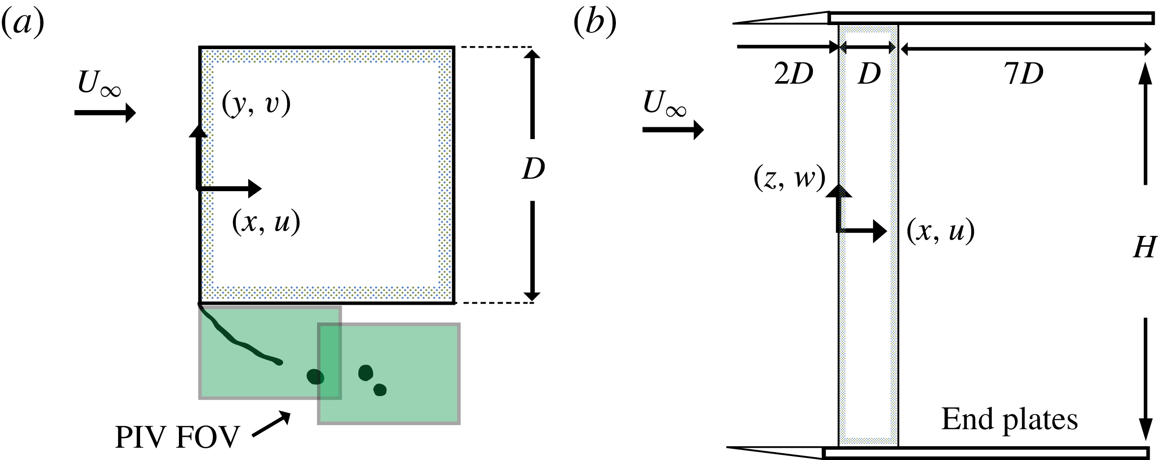
in both cross-stream directions. According to Blackburn & Melbourne (Reference Blackburn and Melbourne1996), a short upstream extension aids in minimising the endplate boundary layer thickness, thus limiting the interaction of horseshoe vortices with the wake vortical structures. Based on the area between the endplates, the blockage ratio was 9.1 %. A schematic of the model in plan and elevation is shown in figure 2.
Experimental set-up: (a) model section indicating the positions of the two particle image velocimetry fields of view (PIV FOV); (b) model plan illustrating the model endplates.

Time-averaged surface pressure measurements were made on the circumference of the prism at centre span (
 $z=0$
) with 12 taps/face using Scanivalve DSA-3217 scanners. The scanners have a sensor range of
 $\pm 10$
inches
 $\text{H}_{2}\text{O}$
(
 $\pm$
0.2 % full-scale static accuracy). One-dimensional velocity measurements were made using a Dantec MiniCTA hot-wire system, sampling at 10 kHz. A single sensor wire probe was used with straight type-55p11,
 $5~\unicode[STIX]{x03BC}\text{m}$
diameter, 1.25 mm long plated tungsten wire. The wire and probe were mounted to a two-axis Velmex BiSlide positioning stage with straight-line positional accuracy of 0.076 mm. Measurements were made at numerous transverse locations through the shear layer in the range
 $0.01<x/D<0.3$
.
As shown in figure 2, two-component particle image velocimetry (PIV) was used at two fields of view (FOV) in the shear layer region. PIV data were obtained in the range
 $16\,700\leqslant Re_{D}\leqslant 148\,000$
. Images were acquired at a sampling rate of
 ${\sim}15$
Hz using a single LaVision Imager LX camera with a
 $1608~\text{pixel}\times 1208~\text{pixel}$
resolution and 12-bit ADC sensor. A Nikon AF Micro-Nikkor 200 mm lens was employed. This resulted in FOV with a spatial extent of
 $0.55D\times 0.41D$
. Seeding particles were vaporised glycol/water-based liquid with mean particle diameter of
 $1~\unicode[STIX]{x03BC}\text{m}$
. Particles were introduced at the tunnel blower inlet, ensuring good mixing and uniformity across the test section. Illumination was provided by a New Wave Solo PIV 120 mJ/pulse per frame Nd:YLF (
 $532~\unicode[STIX]{x03BC}\text{m}$
) dual-head laser. The camera and lasers were controlled and timed using the LaVision Programmable Timing Unit (PTU8). An articulated optical arm was used to guide the laser beam to the required position, where focal and optical lenses spread the beam into a
 ${\sim}1~\text{mm}$
thick sheet.
Estimates of velocities in the FOV were obtained by performing cross-correlations of acquired image pairs. The acquisition timing between images pairs,
 $\unicode[STIX]{x0394}t$
, was based on an eight-pixel shift at the outer edge of the time shear layer, near separation. This resulted in smaller pixel shift within the shear layer and recirculation region; nonetheless, these regions exhibited a single dominant peak in the cross-correlation maps. One thousand image pairs were acquired for each set of operating conditions; with this quantity, convergence of the root mean square of the velocity fluctuations was achieved. A multi-pass correlation setting was employed consisting of a single-pass 32 pixel
 $\times$
32 pixel interrogation window with 50 % overlap followed by a dual-pass 16 pixel
 $\times$
16 pixel interrogation window with 50 % overlap. Post-processing algorithms eliminated spurious vectors and interpolated across them. The post-processed data had a spatial resolution of 0.21 mm/vector.
As noted in Christensen & Scarano (Reference Christensen and Scarano2015), the quality of PIV data is what defines the validity of a subsequent analysis and discussion. It follows that considerations as to the error within a PIV measurement become an integral part of the experiment. Specifically, areas where the error is of a similar order as the measurement itself ought to be avoided. In the current set-up, special attention is paid to the velocity field adjacent to the leading-edge corner. The resulting flow fields captured using the PIV system described above demonstrate the extreme spatial dependence of the velocity, especially close to the leading edge. Past investigations from Neal et al. (Reference Neal, Sciacchitano, Smith and Scarano2015) have shown that the steep spatial velocity gradients within shear layers represent an obstacle for traditional laboratory PIV systems. It is worth noting that the resulting error in shearing regions is larger compared to errors calculated in relatively uniform flows.
Measurement error in PIV represents the difference between a measured velocity vector and the true velocity. Without knowledge of the true value itself, confidence intervals are specified and defined to be an uncertainty (Coleman & Steele Reference Coleman and Steele2009). The error then has a statistical probability of residing within the uncertainty. Methods such as the correlation statistics method, discussed in Wieneke (Reference Wieneke2015), formulate an algorithm to define the uncertainty within an instantaneous PIV snapshot. However, the uncertainty of time-averaged parameters using the definitions in Sciacchitano, Neal & Smith (Reference Sciacchitano, Neal and Smith2015) are more relevant to the analysis at hand and are employed in the following sections. In particular, the uncertainty of the mean velocity field follows the relation
 $U_{\overline{U}}=\unicode[STIX]{x1D70E}_{\overline{U}}/\sqrt{N}$
, where
 $U_{\overline{U}}$
,
 $\unicode[STIX]{x1D70E}_{\overline{U}}$
and
 $N$
are the uncertainty field, the standard deviation of the velocity field and the number of independent samples, respectively. From this form it was found that the highest uncertainties within the velocity fields existed along the centreline of the shear layer. Within a 95 % confidence interval, the mean velocity was everywhere found to have uncertainties less than
 $\pm 4\,\%$
of the free stream,
 $U_{\infty }$
, for all Reynolds numbers tested, and substantially lower uncertainties in areas less affected by shear. Intrinsic to this analysis is the assumption that the individually acquired samples are statistically independent. Furthermore, errors contributing to the uncertainty of the measurement are assumed to be precision based instead of biased. This allows the uncertainty analysis to demonstrate the property of approaching zero with a sufficiently large sample size,
 $N\rightarrow \infty$
. Systematic errors such as camera focus and peak locking were monitored carefully during data acquisition but were not taken into account quantitatively.
3 Results
Results from experiments and simulations are presented in this section. Firstly, § 3.1 presents the frequency ratio scaling obtained from the hot-wire measurements. Subsequently, § 3.2 presents and discusses the spatial evolution of scaling parameters derived from the time-averaged velocity fields. In § 3.3, considerations are made of the development of the front-face boundary layer and the implications for the frequency ratio scaling are considered. In § 3.4 the development of the fluctuating quantities, which demarcate transition characteristics, are observed and discussed. Finally, in § 3.6, some brief considerations are made of scaling at high Reynolds numbers.
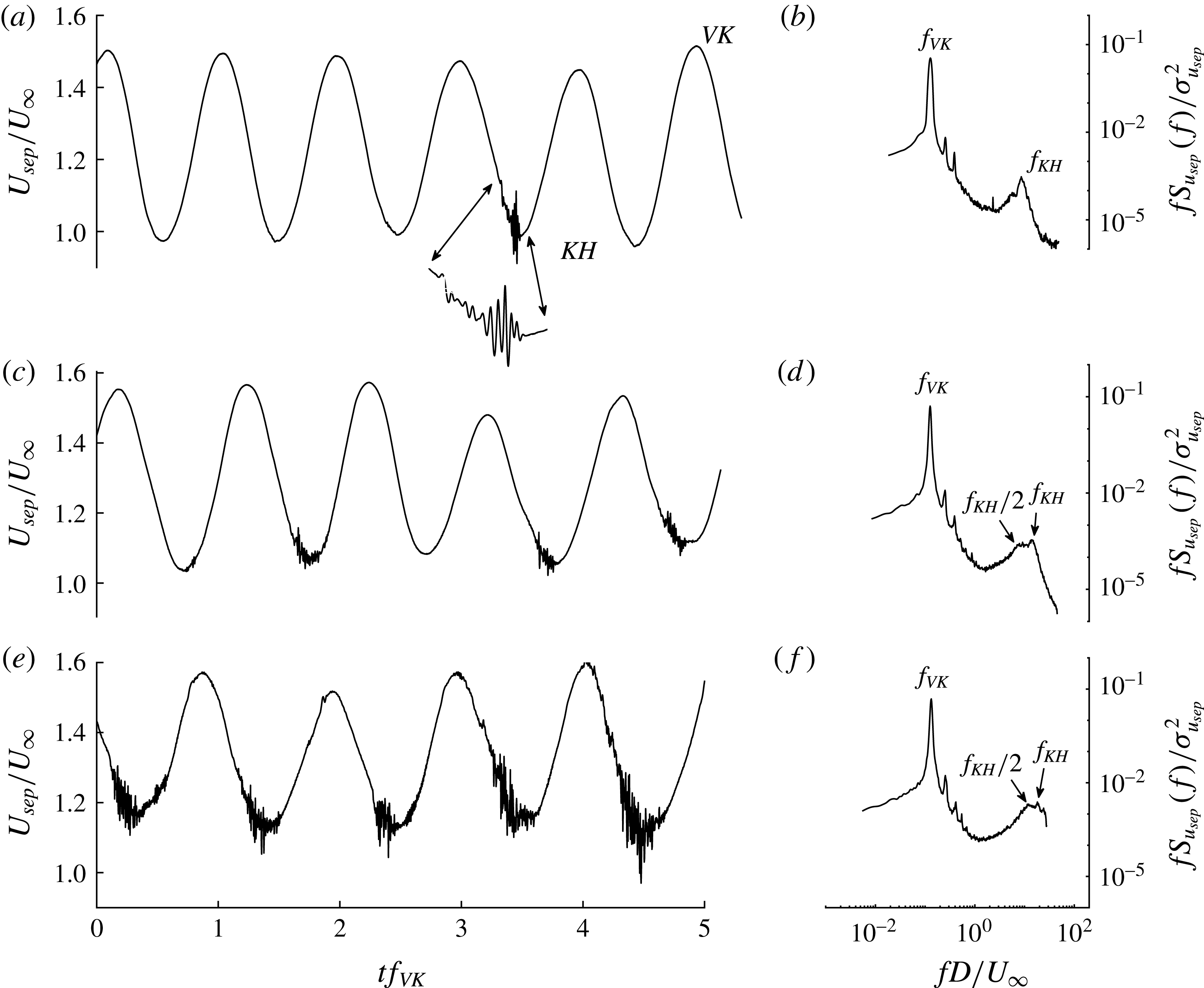
Instantaneous velocity at separation,
 $U_{sep}/U_{\infty }$
, measured in the domain
 $x/D\in \{0.000,0.025\}$
and range
 $y/D\in \{-0.500,-0.505\}$
with a hot wire. Five periods of von Kármán shedding are presented with the corresponding pre-multiplied distributions of power spectral density of the fluctuating velocities,
 $fS_{u_{sep}}(f)/\unicode[STIX]{x1D70E}_{u_{sep}}^{2}$
where
 $\unicode[STIX]{x1D70E}_{u_{sep}}^{2}$
is the variance of the signal. Three Reynolds numbers are presented: (a,b)
 $Re_{D}=21\,400$
; (c,d)
 $Re_{D}=41\,300$
; and (e,f)
 $Re_{D}=71\,000$
.

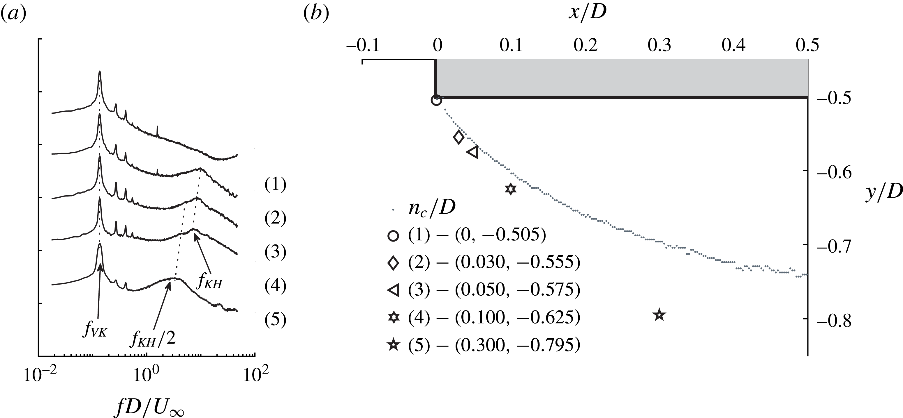
(a) Distributions of pre-multiplied power spectral density of velocity fluctuations near separation,
 $fS_{u_{sep}}(f)/\unicode[STIX]{x1D70E}_{u_{sep}}^{2}$
, where
 $\unicode[STIX]{x1D70E}_{u_{sep}}^{2}$
is the variance of the hot-wire signal presented along the axis of the shear layer at
 $Re_{D}=21\,500$
. Spectral density amplitudes have been linearly shifted on the ordinate to permit the comparison of the energy distribution between cases (1) and (5). (b) The positions of the acquisition in relation to the time-averaged shear layer position,
 $n_{c}$
.

3.1 Frequency ratio scaling
Figure 3 presents time histories and power spectral densities of the velocity near separation, acquired in the domain
 $x/D\in \{0.000,0.025\}$
and range
 $y/D\in \{-0.500,-0.505\}$
for reasons to be explained presently. Three increasing
 $Re_{D}$
cases are presented. The large oscillations in the time traces are caused by the transverse flapping motion of the shear layer, induced by the formation and convection of VK vortices in the wake. The peaks of the VK oscillations occur when the shear layer is laterally closest to the body. Figure 3 demonstrates that the velocity fluctuations at
 $f_{KH}$
appear on the troughs of the VK oscillations; that is, when the shear layer is farthest from the body. The hot wire was intentionally positioned at the outer edge of the shear layer, as this substantially increased the prominence of the spectral peaks at
 $f_{KH}$
. With the hot wire further embedded into the shear layer, the
 $f_{KH}$
peak broadened and became difficult to discern. Examples of the spectrum used to identify
 $f_{KH}$
and
 $f_{VK}$
are shown for each
 $Re_{D}$
in figure 3(b,d,f). At
 $Re_{D}=21\,500$
, the fluctuations at
 $f_{KH}$
appear on one of five troughs, while at
 $Re_{D}=41\,300$
they appear on three. The streamwise variation of the instability inception point, imposed on transverse motion of the shear layer, is the cause of this intermittent appearance, as observed by a stationary pointwise measurement. Prasad & Williamson (Reference Prasad and Williamson1997) addressed the relative energy of peaks corresponding to
 $f_{VK}$
and
 $f_{KH}$
, noting that the intermittency of
 $f_{KH}$
in the hot-wire signal reduced its magnitude, compared to the value which would be expected were it measured continuously. Distributions of power spectral density like that in figure 3(b,d,f) were used to identify
 $f_{KH}$
and
 $f_{VK}$
over the range
 $16\,700\leqslant Re_{D}\leqslant 101\,000$
. However, for
 $Re_{D}>75\,600$
, the magnitude and prominence associated with the KH energy reduced such that there were difficulties identifying a precise frequency. Therefore, the frequency ratio scaling is only presented up to
 $Re_{D}=75\,600$
.
Figure 4(a) presents the development of spectral components at
 $Re_{D}=21\,500$
along the axis of the shear layer at positions indicated in figure 4(b). The spectral density amplitudes have been shifted on the ordinate to permit the comparison of the frequency components. In each acquisition, the hot wire is positioned at the outer edge of the shear layer. Very close to the separation point, the spectrum at (1) has no sign of
 $f_{KH}$
while
 $f_{VK}$
is clearly observed. Traversing to location (2) reveals that spectral energy at
 $f_{KH}$
is now present. At stations farther downstream,
 $f_{KH}$
subharmonics grow in strength until location (5) where
 $f_{KH}/2$
dominates the primary instability due to the pairing process. A distinctive feature of figure 4(a) is that the spectral peaks at
 $f_{KH}$
and
 $f_{KH}/2$
shift to lower frequencies with increasing distance along the shear layer. This is expected to be associated with a slight reduction in the convection speed of the KH vortices as they encounter the region of high curvature beyond separation. The reverse flow on the inner side of the shear layer may also contribute to this reduction. To avoid this migration, for the data presented in figure 3 and in the subsequent analysis, the hot wire was positioned as close to separation as possible where a distinct
 $f_{KH}$
peak could be identified.
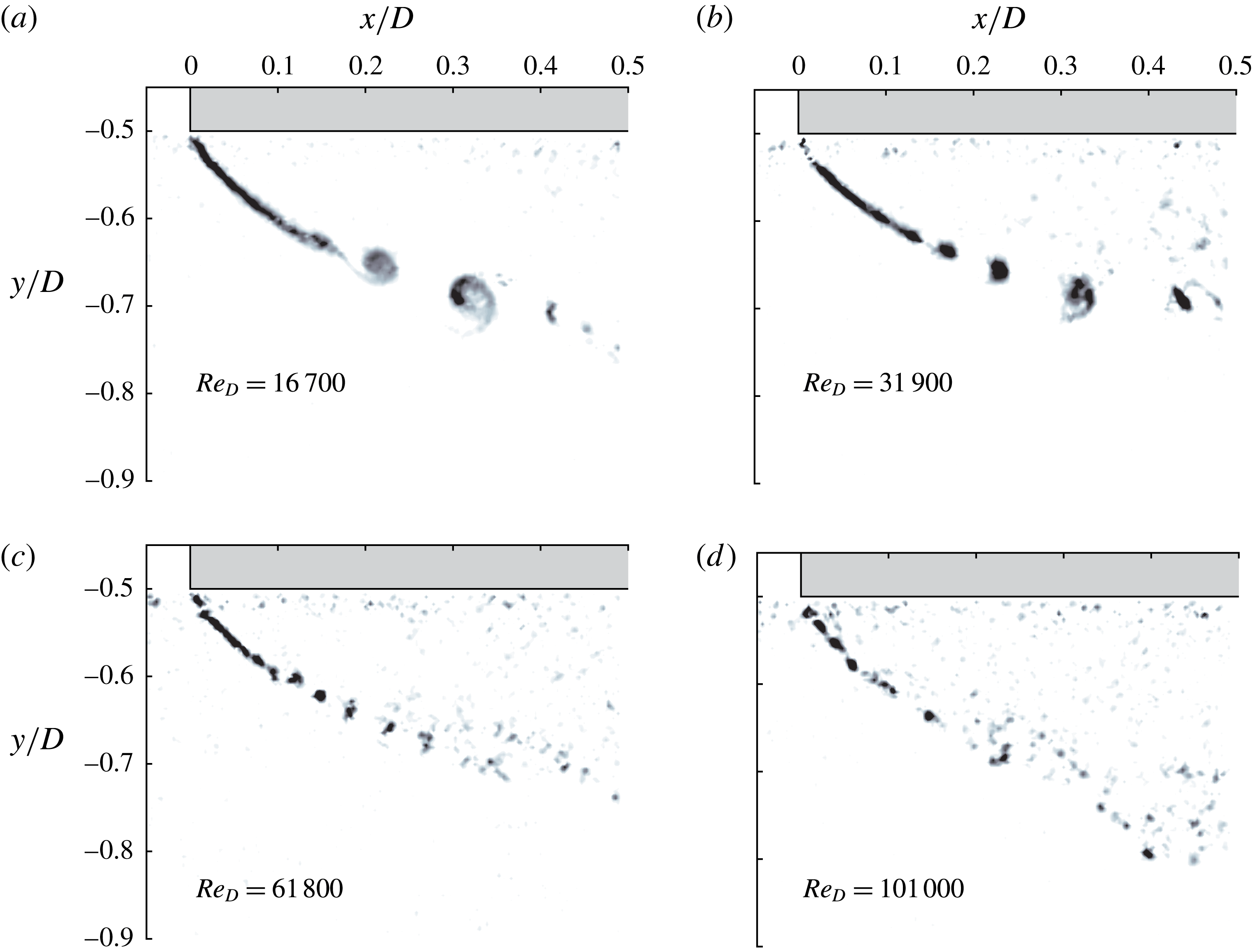
Instantaneous Q criterion for increasing
 $Re_{D}$
.

To complement the above pointwise, time-resolved accounts of the shear layer transition, figure 5(a–d) presents several instantaneous field measurements from the PIV. Here, renderings of Q criterion are presented for increasing
 $Re_{D}$
. In figure 5(a) the evolution of the shear layer transition mechanics are captured with elegance. The KH instability induces an undulation in the laminar shear layer. With increasing distance from separation, the disturbance amplifies before rolling up to form discrete vortices. The structures advance with coherence as they entrain fluid and diffuse vorticity. With farther distance from separation, large deformations in the vorticity distributions cause a breakdown into random eddies. With increasing
 $Re_{D}$
, the transition process moves closer to separation and the size of the vortices forming decreases while the spatial frequency of vortices increases, as shown in figure 5(b–d).
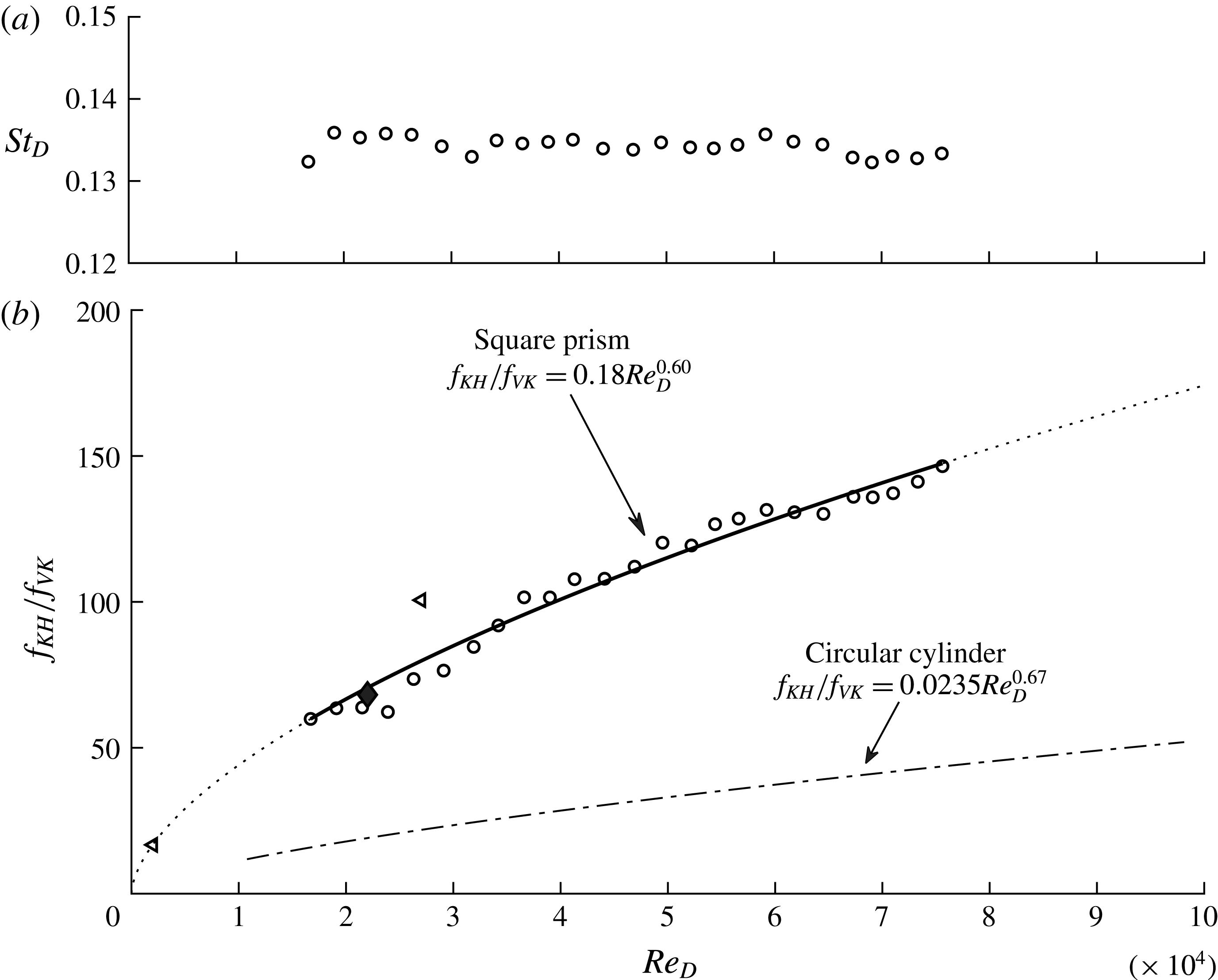
(a) Strouhal-number data. (b) Frequency ratio scaling,
 $f_{KH}/f_{VK}$
, estimated from hot-wire measurements as a function of
 $Re_{D}$
for both the prism (——) and cylinder (— ⋅ —), Prasad & Williamson (Reference Prasad and Williamson1997). Also presented are data of Brun et al. (Reference Brun, Aubrun, Goossens and Ravier2008) (◃), and Trias, Gorobets & Oliva (Reference Trias, Gorobets and Oliva2015) (♦).

Figure 6(a,b) displays the Strouhal number and frequency ratio
 $f_{KH}/f_{VK}$
, respectively, as a function of
 $Re_{D}$
. Figure 6(b) presents data for the prism and the cylinder, according to Prasad & Williamson (Reference Prasad and Williamson1997). In the range
 $16\,700\leqslant Re_{D}\leqslant 75\,600$
,
 $f_{VK}$
increased linearly with
 $U_{\infty }$
such that
 $St_{D}=0.134$
, as presented in figure 6(a), in good agreement with other studies of prisms for
 $Re_{D}>1000$
(Norberg Reference Norberg1993). A robust nonlinear least-squares regression fit to the data was employed which used a least absolute residual method to minimise the effect of outliers. The frequency ratio scaling on the square prism obeys the power-law relation
 $$\begin{eqnarray}\displaystyle \frac{f_{KH}}{f_{VK}}=0.18\,Re_{D}^{0.6}. & & \displaystyle\end{eqnarray}$$
Also presented in figure 6(b) are the data of Brun et al. (Reference Brun, Aubrun, Goossens and Ravier2008) and Trias et al. (Reference Trias, Gorobets and Oliva2015), which are the only data points available in the literature for the prism. These data are at
 $Re_{D}=2000$
(large eddy simulation, LES),
 $Re_{D}=22\,000$
(direct numerical simulation, DNS) and
 $Re_{D}=27\,000$
(laser Doppler velocimetry). At
 $Re_{D}=2000$
, the data agree, while at
 $Re_{D}=27\,000$
, Brun’s data overestimate the current data by 24 %. The present estimation agrees very well with the DNS data of Trias et al. (Reference Trias, Gorobets and Oliva2015), taken at
 $(x/D,y/D)=(0.05,-0.63)$
. Trias et al. (Reference Trias, Gorobets and Oliva2015) report a relatively broadband frequency peak at the shear layer frequency around
 $f_{KH}/f_{VK}=60$
; close inspection of their spectral density distributions reveals that this peak is actually closer to
 $f_{KH}/f_{VK}=68$
, which is the value that has been reported in figure 6. Using LES, Brun et al. (Reference Brun, Aubrun, Goossens and Ravier2008) also noted the presence of a KH vortex at
 $Re_{D}=1000$
, but it was absent at
 $Re_{D}=500$
, which led them to conclude that the onset Reynolds number is within this range for the prism. For parallel shedding conditions on the circular cylinder, the shear layer first manifests at
 $Re_{D}\approx 1200$
(Prasad & Williamson Reference Prasad and Williamson1997).
The magnitude of the frequency ratio of the prism exceeds that for the cylinder for all
 $Re_{D}$
presented in figure 6. As noted in § 1, the aggressive favourable pressure gradient on the front face of the prism creates a thinning boundary layer and therefore a relatively thin initial shear layer. Moreover, the ‘bluffness’ of the square prism increases the wake width and lowers the VK instability frequency by more than 50 %, compared to the cylinder (Roshko Reference Roshko1955). Each of these effects influences the relative magnitudes in figure 6. The exponent of the power law is less for the prism than for the cylinder. Considerations of the physical origins of this parameter are made in subsequent sections. The following section presents the spatial development of parameters relevant to the shear layer scaling which are derived from the time-averaged flow field.
3.2 Development of time-averaged quantities
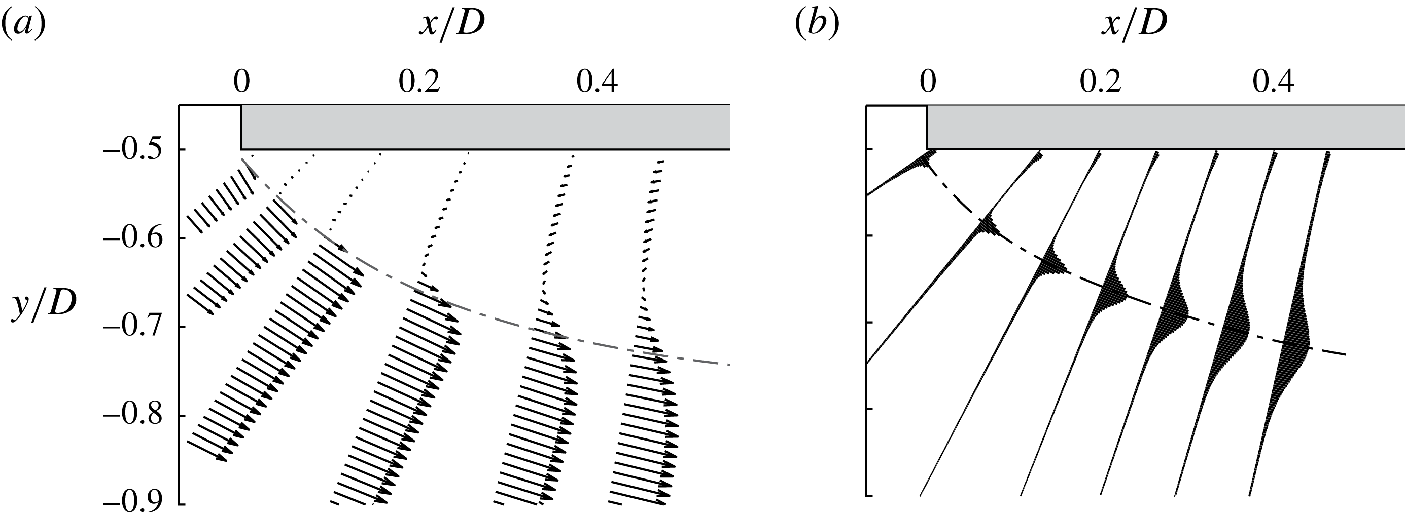
For a prism with no angle of incidence to the flow, the shear layer separates with its axis orthogonal to the free-stream direction. Therefore, a length dominated by pronounced curvature is a unique characteristic of the square-prism shear layer. Accordingly, the axis of the shear layer changes relative to the Cartesian coordinate system as it matures; this feature is in contrast to the plane mixing layer and shear layer of a cylinder, where the time-averaged position naturally develops in the streamwise direction. The time-averaged flow gradients also align with this local axis. Orientation to these local gradients is essential for accurate estimation of parameters such as the momentum thickness, on which the scaling of the KH instability will depend. Accordingly, the present study employs a coordinate system similar to that in Mignot et al. (Reference Mignot, Vinkovic, Doppler and Riviere2014); that is, one locally oriented to the time-averaged shear layer position. Velocity components are interpolated onto profiles which are locally tangential and normal,
 $(s,n)$
, to the time-averaged position of the shear layer centre,
 $n_{c}$
, defined as the trajectory of the maximum fluctuation,
 $(\overline{u^{2}}+\overline{v^{2}})_{max}/2$
. Figure 7(a,b) presents examples of the coordinate system transformation, where the locally tangential profiles of velocity and turbulent kinetic energy are shown. In figure 7(a), the local alignment of velocity vectors to the curved time-averaged shear layer position is apparent. Note the large transverse velocity component on the profile nearest separation. In figure 7(b), the growth and diffusion of fluctuating energy along the axis of the shear layer are apparent.
Locally tangential profiles of velocity (a) and turbulent kinetic energy (b).

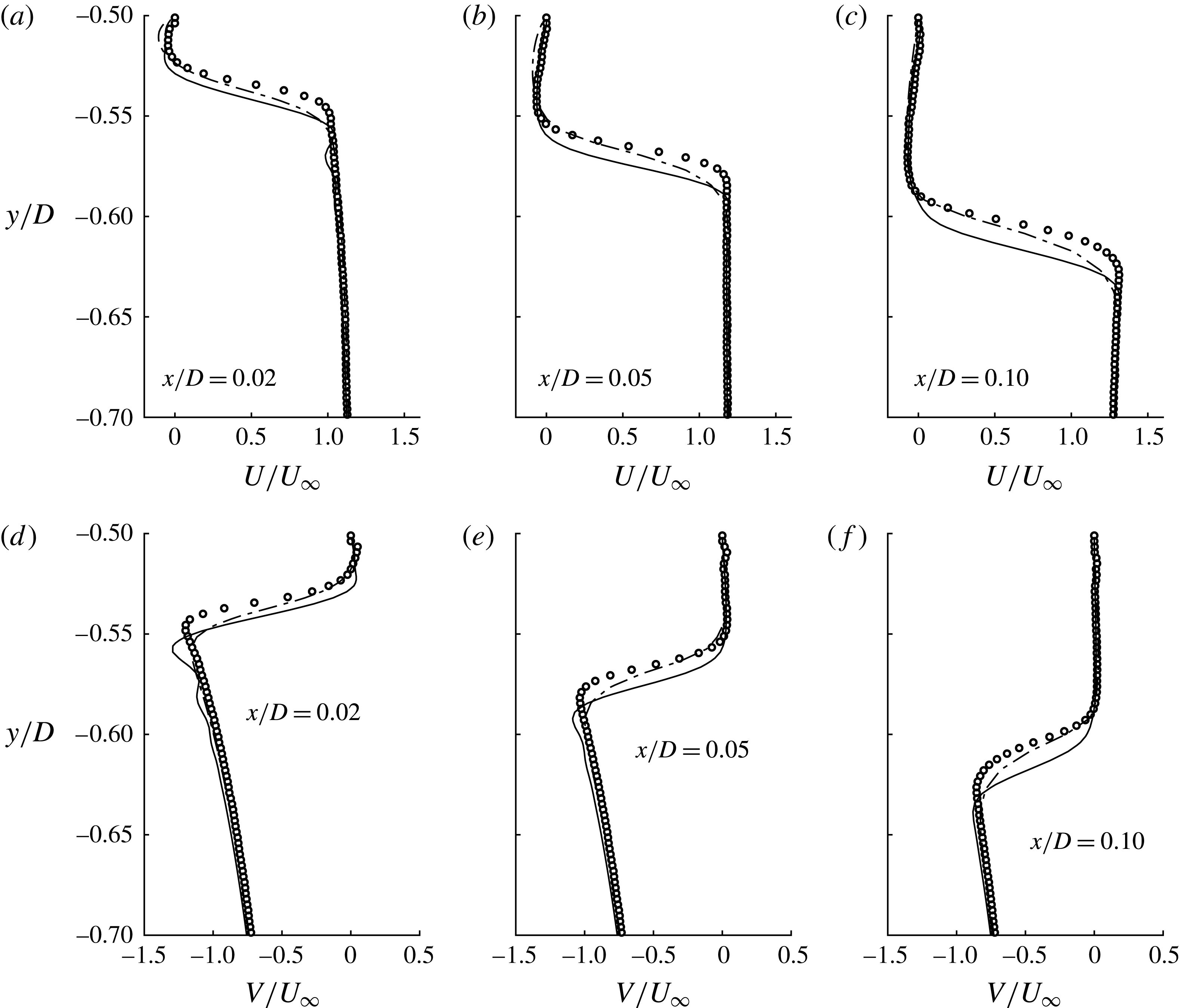
Time-averaged velocity profiles at
 $Re_{D}=21\,500$
at three locations between separation and
 $x/D=0.1$
. (a–c) Streamwise data presented in the Cartesian coordinate system and (d–f) transverse velocity in the same coordinates. Also presented are data of the two DNS studies, Alves Portela, Papadakis & Vassilicos (Reference Alves Portela, Papadakis and Vassilicos2017),
 $Re_{D}=3900$
(— ⋅ —), and Trias et al. (Reference Trias, Gorobets and Oliva2015),
 $Re_{D}=22\,000$
(——).

Figure 8(a–c) presents profiles of time-averaged streamwise velocity at three locations between separation and
 $x/D=0.1$
. Similarly, figure 8(d–f) presents time-averaged transverse velocity on the same profiles. Note that, for ease of comparison, the profiles are presented in the Cartesian coordinate system, while subsequent analysis is conducted in the local system. Also presented in figure 8 are data of two DNS; the data of Alves Portela et al. (Reference Alves Portela, Papadakis and Vassilicos2017) at
 $Re_{D}=3900$
were provided by private communication, while the data of Trias et al. (Reference Trias, Gorobets and Oliva2015) at
 $Re_{D}=22\,000$
are available from a database listed in ref. [36] of their paper. Data from the current study in figure 8 are at
 $Re_{D}=21\,500$
.
Streamwise development of time-averaged flow parameters in the shear layer region. (a) The time-averaged streamlines with shear layer position,
 $n_{c}$
, and the trajectories of maximum inner (
 $i$
) and outer (
 $o$
) tangential velocities,
 $U_{s}$
. (b) The development of
 $U_{s_{o}}$
and
 $U_{s_{i}}$
in the streamwise direction; and (c) the velocity ratio,
 $R$
, for two Reynolds numbers. These data are calculated from the local coordinate system.

For both profiles of the streamwise and transverse velocity components, the experiments and simulations agree, with some notable differences. The DNS of Trias et al. (Reference Trias, Gorobets and Oliva2015), which is at comparable Reynolds number, has its maximum velocity gradient,
 $\unicode[STIX]{x2202}U/\unicode[STIX]{x2202}y$
, farther from the wall, compared to the experimental data. The different position of maximum
 $\unicode[STIX]{x2202}U/\unicode[STIX]{x2202}y$
asserts that the DNS data predict that the time-averaged location of the shear layer is further from the body. Differences in blockage ratio (9 %, present; 2 %, Trias et al. (Reference Trias, Gorobets and Oliva2015)), levels of free-stream turbulence (0.3 %, present; 0 %, Trias et al. (Reference Trias, Gorobets and Oliva2015)) and geometric model imperfections at the leading edge may explain why the time-averaged position of the experimental data track closer to the body. It is also apparent that the transverse velocity of Trias et al. (Reference Trias, Gorobets and Oliva2015) is slightly larger than the present observations outside the shear layer; this discrepancy decreases farther into the free stream. At each streamwise position, the data of Alves Portela et al. (Reference Alves Portela, Papadakis and Vassilicos2017) appear to have a less severe gradient,
 $\unicode[STIX]{x2202}U/\unicode[STIX]{x2202}y$
, in the region of shear, indicating slight
 $Re_{D}$
effects within the shear layer.
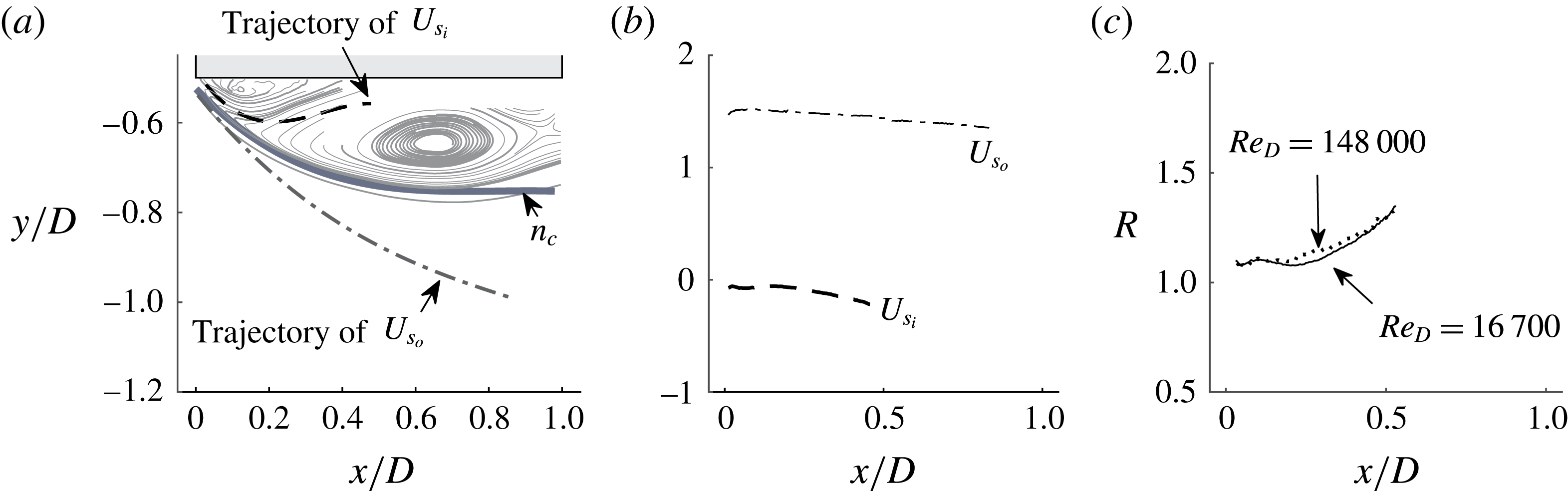
Figure 9(a) presents the location of the time-averaged shear layer position,
 $n_{c}$
, over streamlines. The position of the shear layer undergoes large unsteady ‘flapping’ around the time-averaged position at the VK frequency (Lyn & Rodi Reference Lyn and Rodi1994; Lander et al.
Reference Lander, Letchford, Amitay and Kopp2016). Trajectories of the time-averaged local maximum tangent velocities,
 $U_{s}$
, on the inner (
 $i$
) and outer (
 $o$
) sides of the shear layer are also presented. The path of
 $U_{s_{i}}$
is over the outer edge of a small clockwise-rotating leading-edge recirculation bubble and between the main anticlockwise-rotating recirculation region and the prism side face. Figure 9(b) presents the variation of the maximum outer and inner velocities with downstream distance at
 $Re_{D}=16\,700$
. The maximum outer velocity,
 $U_{s_{o}}$
, follows a trajectory into the free stream and is almost constant at
 $U_{s_{o}}/U_{\infty }\simeq 1.45$
. The inner tangential velocity is negative, varying between 7 % and 21 % of the free stream over the observable domain. In figure 9(c), the velocity ratio
 $R=\unicode[STIX]{x0394}U_{s}/2\overline{U}_{s}$
is presented, where the mean velocity difference is
 $\unicode[STIX]{x0394}U_{s}=U_{s_{o}}-U_{s_{i}}$
and the average velocity across the shear layer is
 $\overline{U}_{s}=(U_{s_{o}}+|U_{s_{i}}|)/2$
. The velocity ratio increases from 1.09 to 1.35 with increasing distance from separation. The velocity ratio varies only slightly over the range of Reynolds numbers tested. When
 $R>1$
there is reverse flow; moreover, when
 $R>1.315$
, the plane mixing layer becomes absolutely unstable (Huerre & Monkewitz Reference Huerre and Monkewitz1985). This is in contrast to coflowing stream mixing layers and shear layers (
 $R<1$
) where the KH instability develops spatially as a convective instability. For cases with large reverse flow, Huerre & Monkewitz (Reference Huerre and Monkewitz1985) reported that the mixing layer should be described in terms of a temporally growing disturbance, rather than a convective one. Furthermore, Monkewitz & Nguyen (Reference Monkewitz and Nguyen1987) discuss the suppressing influence of curvature on the growth rates of the KH instability. Exploration of these characteristics from a stability orientation is beyond the scope of this investigation; nonetheless, they are mentioned to elucidate the complex environment in which instability of the square-prism shear layer arises.
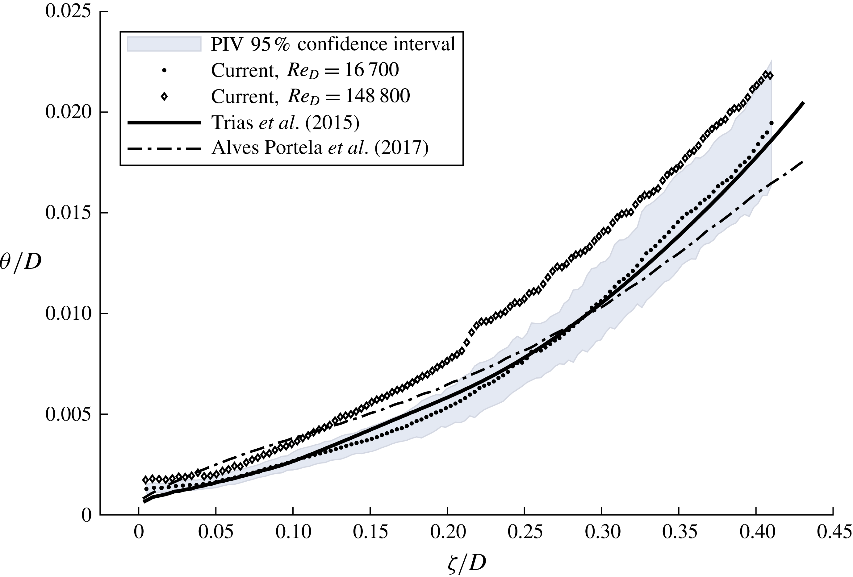
Growth of the momentum thickness along the arclength,
 $\unicode[STIX]{x1D701}$
, of the shear layer at
 $Re_{D}=16\,700$
and 148 000. DNS data of Trias et al. (Reference Trias, Gorobets and Oliva2015) at
 $Re_{D}=22\,000$
and Alves Portela et al. (Reference Alves Portela, Papadakis and Vassilicos2017) at
 $Re_{D}=3900$
are also presented. The 95 % confidence intervals on
 $\unicode[STIX]{x1D703}$
at
 $Re_{D}=16\,700$
are shaded.

Figure 10 presents the momentum thickness of the shear layer at
 $Re_{D}=16\,700$
and
 $148\,000$
as a function of the arclength,
 $\unicode[STIX]{x1D701}/D$
. The DNS data of Trias et al. (Reference Trias, Gorobets and Oliva2015) and Alves Portela et al. (Reference Alves Portela, Papadakis and Vassilicos2017) are also presented in figure 10. The momentum thickness is defined for a shear layer in the local coordinate system as
 $$\begin{eqnarray}\displaystyle \unicode[STIX]{x1D703}=\int \frac{U_{s}(n)-U_{s_{i}}}{U_{s_{o}}-U_{s_{i}}}\left(1-\frac{U_{s}(n)-U_{s_{i}}}{U_{s_{o}}-U_{s_{i}}}\right)\text{d}n. & & \displaystyle\end{eqnarray}$$
The integration limits are adjusted to the position of the maximum inner and outer velocity, on the local profile. This form of the momentum thickness accounts for the reverse flow, which is an important feature of the prism shear layer. Additionally, the uncertainty band defining the 95 % confidence interval is displayed for
 $Re_{D}=16\,700$
in figure 10. This is generated by propagating the highest uncertainties found in the velocity field through (3.2) using the general uncertainty methods in Coleman & Steele (Reference Coleman and Steele2009). The sensitivity variables in that analysis are each of the terms in (3.2) with the exception of the spatial coordinate which is assumed to have uncertainties much less than that of the velocity. In figure 10, the 95 % confidence interval of
 $\unicode[STIX]{x1D703}$
is
 $\pm 18.2\,\%$
of the estimated value at each
 $\unicode[STIX]{x1D701}/D$
. Near separation, where
 $\unicode[STIX]{x1D70E}_{\overline{U}}$
is small compared to farther along the shear layer, these uncertainty bounds are very conservative. The uncertainty band for
 $Re_{D}=148\,800$
has a similar width, but has been omitted for visual clarity.
As shown in figure 8, velocity profiles in the region
 $\unicode[STIX]{x1D701}/D<0.1$
exhibit asymmetry around an inflection point at the shear layer centre. The outer flow is accelerated above
 $U_{\infty }$
and contains a ‘knee’ feature, while the inner flow takes a trajectory through the recirculation region. The velocity profile in figure 1 schematically illustrates these features. Where velocity profiles fit the hyperbolic tangent function, it is easily shown that the ratio of the vorticity to momentum thickness is
 $\unicode[STIX]{x1D6FF}_{\unicode[STIX]{x1D714}}/\unicode[STIX]{x1D703}=4$
(Monkewitz Reference Monkewitz1982); for profiles with asymmetry, this factor is other than 4 and dependent on the shape of the profile. For the present data, when
 $0<\unicode[STIX]{x1D701}/D\lesssim 0.5$
, the ratio is initially larger than 4, but subsequently decays with increasing streamwise distance; for
 $\unicode[STIX]{x1D701}/D\gtrsim 0.5$
,
 $\unicode[STIX]{x1D6FF}_{\unicode[STIX]{x1D714}}/\unicode[STIX]{x1D703}=4$
. It follows that, in the initial region of the shear layer, one cannot interchange
 $\unicode[STIX]{x1D6FF}_{\unicode[STIX]{x1D714}}$
and
 $\unicode[STIX]{x1D703}$
and expect a consistent scaling argument. We maintain that the momentum thickness is the more robust length scale, as it is an integral parameter which implicitly includes the influence of the asymmetry of the velocity profile.
In figure 10, the comparison between the experimental data at
 $Re_{D}=16\,700$
and the DNS at
 $Re_{D}=22\,000$
is noteworthy, as both data exhibit similar trends of nonlinear growth. A power law with an exponent larger than one describes this growth for
 $\unicode[STIX]{x1D701}/D>0.05$
. For the DNS of Trias et al. (Reference Trias, Gorobets and Oliva2015), at
 $\unicode[STIX]{x1D701}/D<0.05$
, there appears to be a region of nonlinear growth with an exponent less than one, indicative of an initial length of laminar growth, where the width should increase like
 $\unicode[STIX]{x1D701}^{1/2}$
(Winant & Browand Reference Winant and Browand1974). This observation is corroborated by the DNS of Alves Portela et al. (Reference Alves Portela, Papadakis and Vassilicos2017) at
 $Re_{D}=3900$
where the laminar growth region is extended farther downstream. Nonetheless, by
 $\unicode[STIX]{x1D701}/D\approx 0.25$
, the growth of this low-Reynolds-number case also inflects upwards. Such growth characteristics are more complex than those observed in plane mixing layers, where the initial laminar growth region is followed by a linear turbulent growth region.
In figure 10 the momentum thickness near separation,
 $\unicode[STIX]{x1D703}_{sep}$
, approaches an asymptotic value for
 $\unicode[STIX]{x1D701}/D<0.05$
for both experimental cases presented. This contradicts physical scaling requirements of laminar flows. Conversely, for both DNS cases,
 $\unicode[STIX]{x1D703}_{sep}$
continues thinning to the leading edge. Inspection of the velocity profiles very close to the leading edge clarifies several differences between the measurements and simulations. An underestimation of the velocity gradient by the PIV is the primary cause of the discrepancy. Further attention reveals that the position of
 $U_{s_{i}}$
on the profile, the maximum inner velocity, is closer to the body (farther away from the shear layer centre) in the experiments, compared to the DNS. That is, the region of shear is broader and is attributable to an underestimation of the velocity gradient on the inner side. Since the limits of integration of (3.2) adjust to the local position of
 $U_{s_{i}}$
and
 $U_{s_{o}}$
, the effect is an integration performed over an extended width and an overestimation of
 $\unicode[STIX]{x1D703}_{sep}$
, as observed in figure 10.
Experimental constraints such as beam reflection and inadequate seeding of the low-speed side of the shear layer are suspected to limit the PIV in ways concomitant with the above discussion. Nonetheless, the confidence intervals presented in figure 10 do not fully account for the discrepancy between PIV and DNS. Differences between numerical and experimental set-ups may also contribute; for example, effects related to free-stream turbulence levels and differences in the leading-edge corner radii may contribute to the observed differences. Furthermore, the most severe shear observed in the DNS of Trias et al. (Reference Trias, Gorobets and Oliva2015) at
 $Re_{D}=22\,000$
acts over a distance of
 $0.0044D$
while the resolution of the PIV is only
 $0.0028D$
. Clearly, the spatial resolution obtained using the 16 pixel
 $\times$
16 pixel interrogation window is insufficient to resolve the severe gradients immediately downstream of separation. One also recognises that
 $\unicode[STIX]{x1D703}_{sep}$
is slightly larger for the measured case at
 $Re_{D}=148\,000$
compared to
 $Re_{D}=16\,700$
, although both exhibit the same asymptotic behaviour. Assuming that the front-face boundary layer remains laminar at all tested
 $Re_{D}$
, as argued by Sigurdson (Reference Sigurdson1986), the momentum thickness at separation must decrease in width with increasing
 $Re_{D}$
. Thus, the observed differences of
 $\unicode[STIX]{x1D703}_{sep}$
between the two experimental cases are probably due to experimental difficulties, exacerbated by more severe gradients at larger
 $Re_{D}$
. In comparison, between the two DNS cases,
 $Re_{D}$
shows a sustained influence on the thickness of
 $\unicode[STIX]{x1D703}_{sep}$
.
Returning to the scaling argument, as discussed in § 1, the parameter driving the nonlinearity of
 $f_{KH}/f_{VK}$
proposed by Bloor (Reference Bloor1964) was the boundary layer thickness at separation. The implications of the above observations make clear that experimental limitations preclude the use of
 $\unicode[STIX]{x1D703}_{sep}$
as a scaling parameter of
 $f_{KH}/f_{VK}$
in the present study. However, the sustained influence of
 $Re_{D}$
on
 $\unicode[STIX]{x1D703}_{sep}$
observed in the two DNS studies suggest, similarly to the cylinder, that the nonlinear scaling of
 $f_{KH}/f_{VK}$
must originate in the boundary layer, before separation. Therefore, the following section considers the development of the front-face boundary layer in an effort to understand its influence on the physical origins of the
 $f_{KH}/f_{VK}$
scaling.
3.3 Front-face boundary layer
In this section, the development of the front-face boundary layer is explored with the data of Trias et al. (Reference Trias, Gorobets and Oliva2015) and Alves Portela et al. (Reference Alves Portela, Papadakis and Vassilicos2017). In addition, the data of Sigurdson (Reference Sigurdson1986), who estimated the momentum thickness of the front-face boundary layer,
 $\unicode[STIX]{x1D703}_{BL}$
, for a coaxially aligned blunt-faced cylinder, are presented. Sigurdson (Reference Sigurdson1986) employed the semi-empirical axisymmetric Thwaites method in conjunction with the notched-hodograph theory of Roshko (Reference Roshko1954) which employed the experimental data of Koenig (Reference Koenig1978).
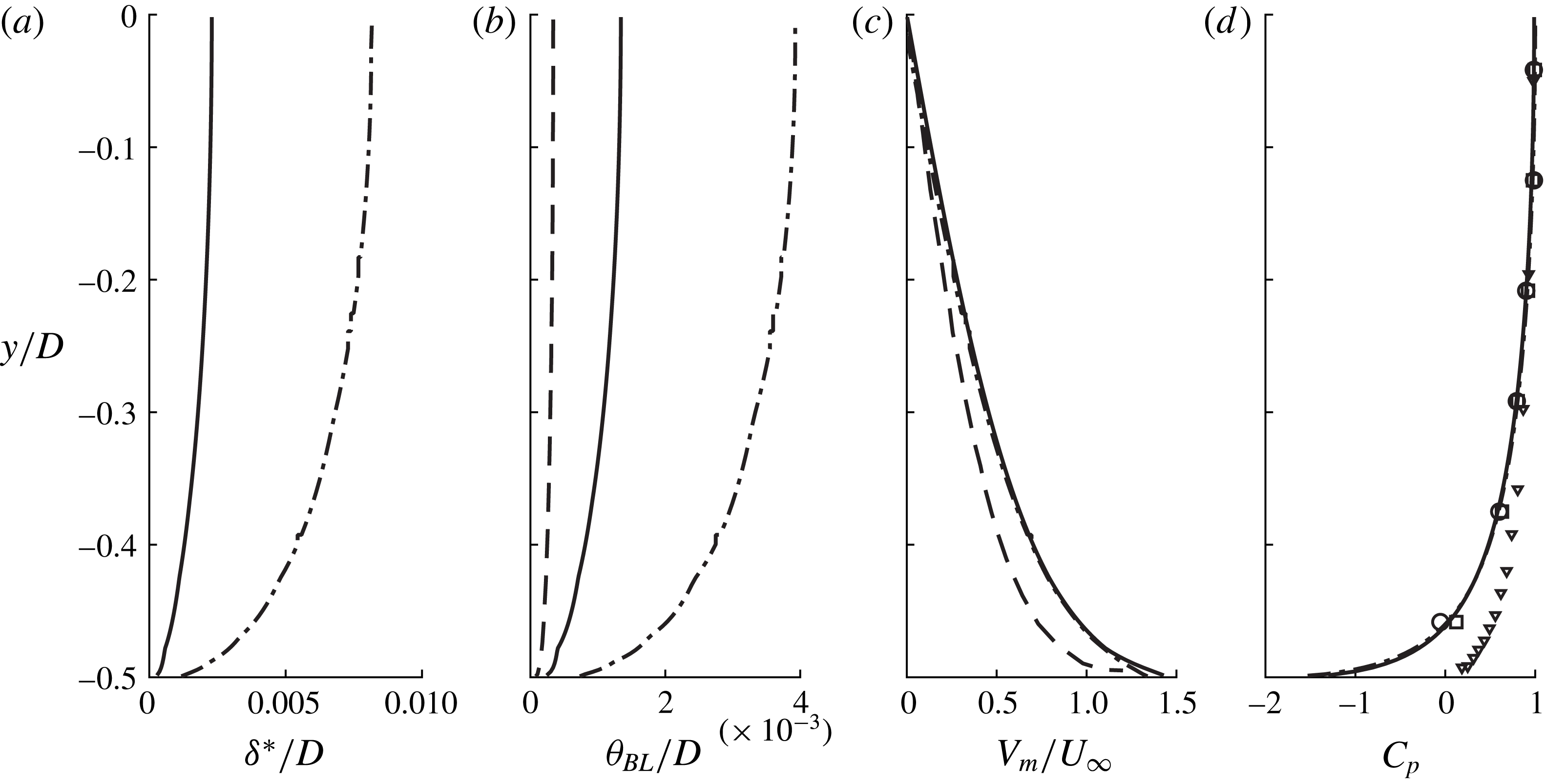
Development of parameters relevant to the front-face boundary layer presented between stagnation (
 $y=0$
) and separation (
 $y=-0.5$
): (a) the boundary layer displacement thickness,
 $\unicode[STIX]{x1D6FF}^{\ast }$
; (b) the boundary layer momentum thickness,
 $\unicode[STIX]{x1D703}_{BL}$
; (c) the maximum transverse velocity,
 $V_{m}$
; and (d) the pressure coefficient on the front face. Data presented are of Trias et al. (Reference Trias, Gorobets and Oliva2015),
 $Re_{D}=22\,000$
(——); Alves Portela et al. (Reference Alves Portela, Papadakis and Vassilicos2017),
 $Re_{D}=3900$
(— ⋅ —); Sigurdson (Reference Sigurdson1986),
 $Re_{D}=500\,000$
(– – –); Koenig (Reference Koenig1978),
 $Re_{D}=500\,000$
(▿); present,
 $Re_{D}=16\,700$
(○); and present,
 $Re_{D}=148\,000$
(▫).

Figure 11 presents several parameters of the front-face boundary layer. The front-face boundary layer develops between stagnation (
 $y=0$
) and separation (
 $y=-0.5$
) as the free-stream flow impinges on the body. Accordingly, the appropriate estimations of the boundary layer parameters are those for a wall jet, rather than a regular boundary layer. Figure 11(a) presents the development of
 $\unicode[STIX]{x1D6FF}^{\ast }$
, the boundary displacement layer thickness between stagnation, near
 $y/D=0$
, and separation at
 $y/D=-0.5$
. The boundary layer displacement thickness is calculated as
 $$\begin{eqnarray}\displaystyle \unicode[STIX]{x1D6FF}^{\ast }=\int _{0}^{\unicode[STIX]{x1D6FF}}\left(1-\frac{V(x)}{V_{m}}\right)\text{d}x, & & \displaystyle\end{eqnarray}$$
where
 $V_{m}$
is the maximum transverse velocity of the impinging flow and
 $\unicode[STIX]{x1D6FF}$
is its distance from the wall. Only the DNS data are presented in figure 11(a). Between stagnation and separation, as predicted analytically by Sigurdson (Reference Sigurdson1986), the boundary layer is observed to thin to a very small width. Furthermore, the influence of
 $Re_{D}$
is starkly observable; the size of
 $\unicode[STIX]{x1D6FF}^{\ast }$
for the high-
 $Re_{D}$
case is much thinner than for the low Reynolds number, corroborating the observed influence of
 $Re_{D}$
on
 $\unicode[STIX]{x1D703}_{sep}$
in the previous section. Figure 11(b) presents the development of
 $\unicode[STIX]{x1D703}_{BL}$
, the boundary layer momentum thickness, which is calculated as
 $$\begin{eqnarray}\displaystyle \unicode[STIX]{x1D703}_{BL}=\int _{0}^{\unicode[STIX]{x1D6FF}}\frac{V(x)}{V_{m}}\left(1-\frac{V(x)}{V_{m}}\right)\text{d}x. & & \displaystyle\end{eqnarray}$$
Figure 11(b) also includes the estimation of Sigurdson (Reference Sigurdson1986) which is based on the data of Koenig (Reference Koenig1978) at
 $Re_{D}=500\,000$
. The
 $Re_{D}$
value maintains influence on the front-face boundary to large values. Figure 11(c,d) presents the maximum transverse velocity,
 $V_{m}$
, and pressure on the front face, respectively. Geometric differences of the square prism and coaxial blunt cylinder are accentuated by the evolution of
 $V_{m}$
in figure 11(c) and pressure in figure 11(d). Indeed, despite sharing the bluff front face and salient leading edges, the pressure gradient and maximum transverse velocities differ increasingly with proximity to separation. The pressure on the coaxial cylinder decreases at a slower rate than the prism; according to the experimental observations of Koenig (Reference Koenig1978), the front-face pressure never falls below the static pressure of the free stream. However, presumably, a precipitous drop in pressure occurs very close to separation, beyond the spatial resolution of the pressure measurements. The maximum transverse velocities estimated by Sigurdson (Reference Sigurdson1986) exhibit agreeable differences, with
 $\unicode[STIX]{x2202}V_{m}/\unicode[STIX]{x2202}y$
increasing more aggressively with proximity to separation. Pressure data of the present study at
 $Re_{D}=16\,700$
and
 $Re_{D}=148\,000$
presented in figure 11(d) exhibit excellent agreement with the DNS data of Trias et al. (Reference Trias, Gorobets and Oliva2015) and Alves Portela et al. (Reference Alves Portela, Papadakis and Vassilicos2017). Here,
 $C_{p}$
decreases abruptly on the front face near separation; indeed, the pressure gradient,
 $\unicode[STIX]{x2202}(C_{p})/\unicode[STIX]{x2202}y$
, and even higher-order derivatives maintain aggressively changing magnitudes with proximity to separation. Accordingly, the production of vorticity in this region will be substantial (Morton Reference Morton1984). The influence of the salient edge on the local velocities and gradients is a defining feature of this flow.
Using the estimations of
 $\unicode[STIX]{x1D703}_{BL}$
presented in figure 11(b), the influence of
 $Re_{D}$
on the front-face boundary layer may be estimated. Here, the data of the two DNS studies and the semi-empirical estimate of Sigurdson (Reference Sigurdson1986) span more than two orders of magnitude of
 $Re_{D}$
using three data points. The different gradients of pressure and maximum transverse velocity of the coaxial cylinder will impact the estimation of
 $\unicode[STIX]{x1D703}_{BL}$
and thereby obscure a precise scaling prediction of the influence of
 $Re_{D}$
on
 $\unicode[STIX]{x1D703}_{BL}$
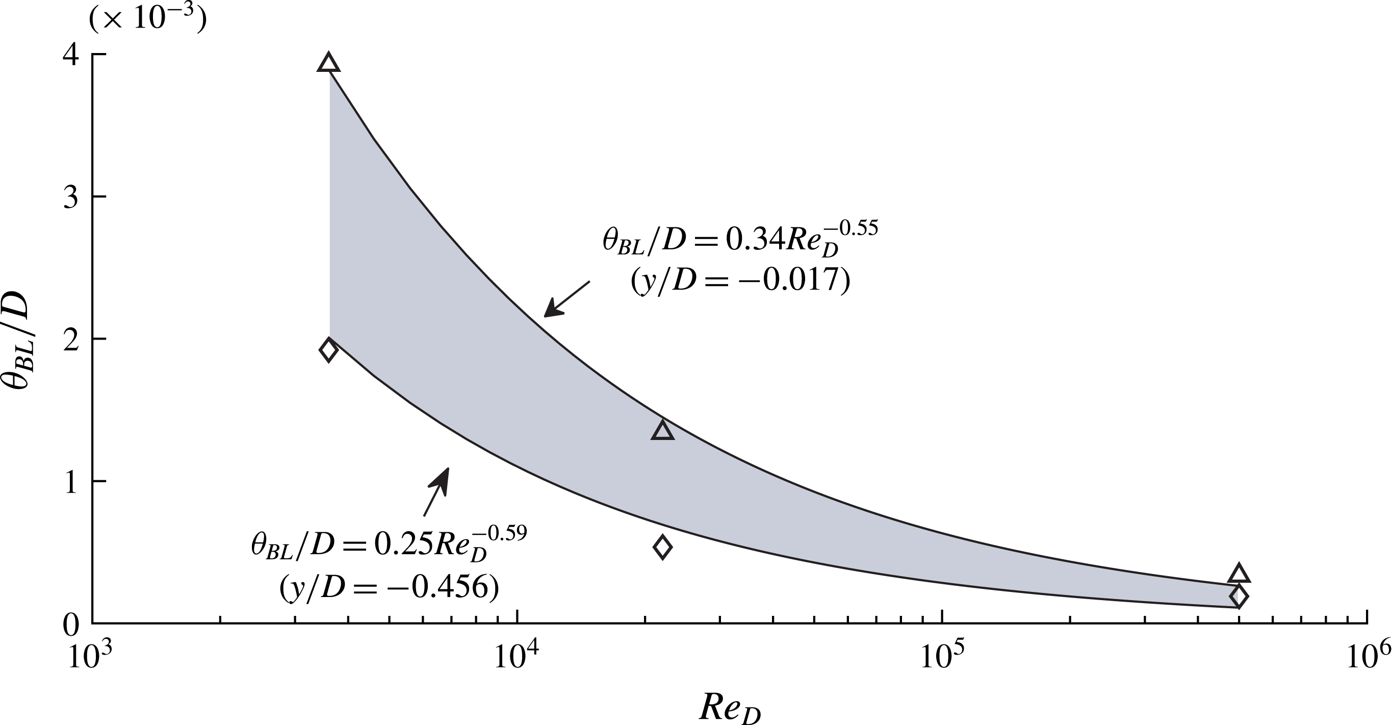
for the square prism. Nonetheless, using the data of figure 11(b), a scaling prediction may be made. We emphasise the need for prudence with extending this scaling argument as a representation of the true physics of the laminar front-face boundary layer of the square prism. In figure 12, a power-law best fit is included for the data at
 $y/D=-0.017$
(stagnation) where the data decay with power law
 $\unicode[STIX]{x1D703}_{BL}/D=0.34\,Re_{D}^{-0.55}$
. Closer to separation, at
 $y/D=-0.456$
, where the boundary layer has thinned, the best fit to the data is
 $\unicode[STIX]{x1D703}_{BL}/D=0.25\,Re_{D}^{-0.59}$
. The shaded area represents the data between these limits. Considering all data available along the front face, the averaged estimated scaling is
 $$\begin{eqnarray}\displaystyle \frac{\unicode[STIX]{x1D703}_{BL}}{D}\propto \frac{1}{Re_{D}^{0.57}}. & & \displaystyle\end{eqnarray}$$
The front-face boundary layer momentum thickness,
 $\unicode[STIX]{x1D703}_{BL}$
, presented as a function of Reynolds number:
 $Re_{D}=3900$
, Alves Portela et al. (Reference Alves Portela, Papadakis and Vassilicos2017);
 $Re_{D}=22\,000$
, Trias et al. (Reference Trias, Gorobets and Oliva2015);
 $Re_{D}=500\,000$
, Sigurdson (Reference Sigurdson1986).

Reflecting once more on the scaling argument of
 $f_{KH}/f_{VK}$
, it is apparent that the exponent in (3.5) is only slightly larger than that proposed by Bloor (Reference Bloor1964). Bloor’s scaling was based on the analytical solution for a laminar boundary layer, which holds true for boundary layers with and without pressure gradients. It follows that
 $\unicode[STIX]{x1D703}_{BL}$
is expected to scale with an exponent close to 0.5. Of course, caution must be maintained with reaching definitive conclusions from (3.5); nonetheless, the trends are illuminating. Referring again to the basic length–velocity scaling argument of (1.1), as discussed in § 1, the frequency ratio scaling can be balanced by an appropriately selected pair of ratios,
 $U/L$
, chosen to represent the KH and VK instabilities. With respect to VK, unlike the cylinder, for the prism, when
 $Re_{D}>1000$
,
 $f_{VK}$
increases linearly with
 $U_{\infty }$
such that
 $St_{D}=0.134$
(Norberg Reference Norberg1993). The critical
 $Re_{D}$
where the KH instability first manifests is also
 $Re_{D}\approx 1000$
(Brun et al.
Reference Brun, Aubrun, Goossens and Ravier2008); hence, the KH instability is not expected to be present within the range where
 $St_{D}$
exhibits
 $Re_{D}$
dependence. It follows that
 $St_{D}$
need not appear in the scaling relationship, and the appropriate length and velocity scales of the VK instability are simply the body diameter and the free-stream velocity, i.e.
 $f_{VK}\propto U_{\infty }/D$
. We note that the derived scaling argument seeks to match the power of (3.1) and not the coefficient, as this is dependent on the particular length and velocity scales employed. Assuming
 $U_{VK}=U_{\infty }$
presently, as suggested by Bloor (Reference Bloor1964), which will be justified in the following section, using the exponent estimated for
 $\unicode[STIX]{x1D703}_{BL}$
, the frequency ratio scaling can be stated as
 $$\begin{eqnarray}\displaystyle \frac{f_{KH}}{f_{VK}}\propto \frac{D}{\unicode[STIX]{x1D703}_{BL}}\propto Re_{D}^{0.57}. & & \displaystyle\end{eqnarray}$$
It is apparent that, as for the cylinder, the frequency ratio scaling of (3.1) is in part dependent on the influence of
 $Re_{D}$
on the boundary layer prior to separation. Unfortunately, PIV measurements on the front face are precluded with the diagnostic tools available, for the limitations discussed in § 3.2. As such, the findings presented in this section cannot be experimentally validated. Nonetheless, it is possible to observe characteristics of the KH instability downstream of separation, which may corroborate the relations observed on the front face. The following section explores the shear layer scaling by consideration of the parameters derived from the spatial development of fluctuating velocities.
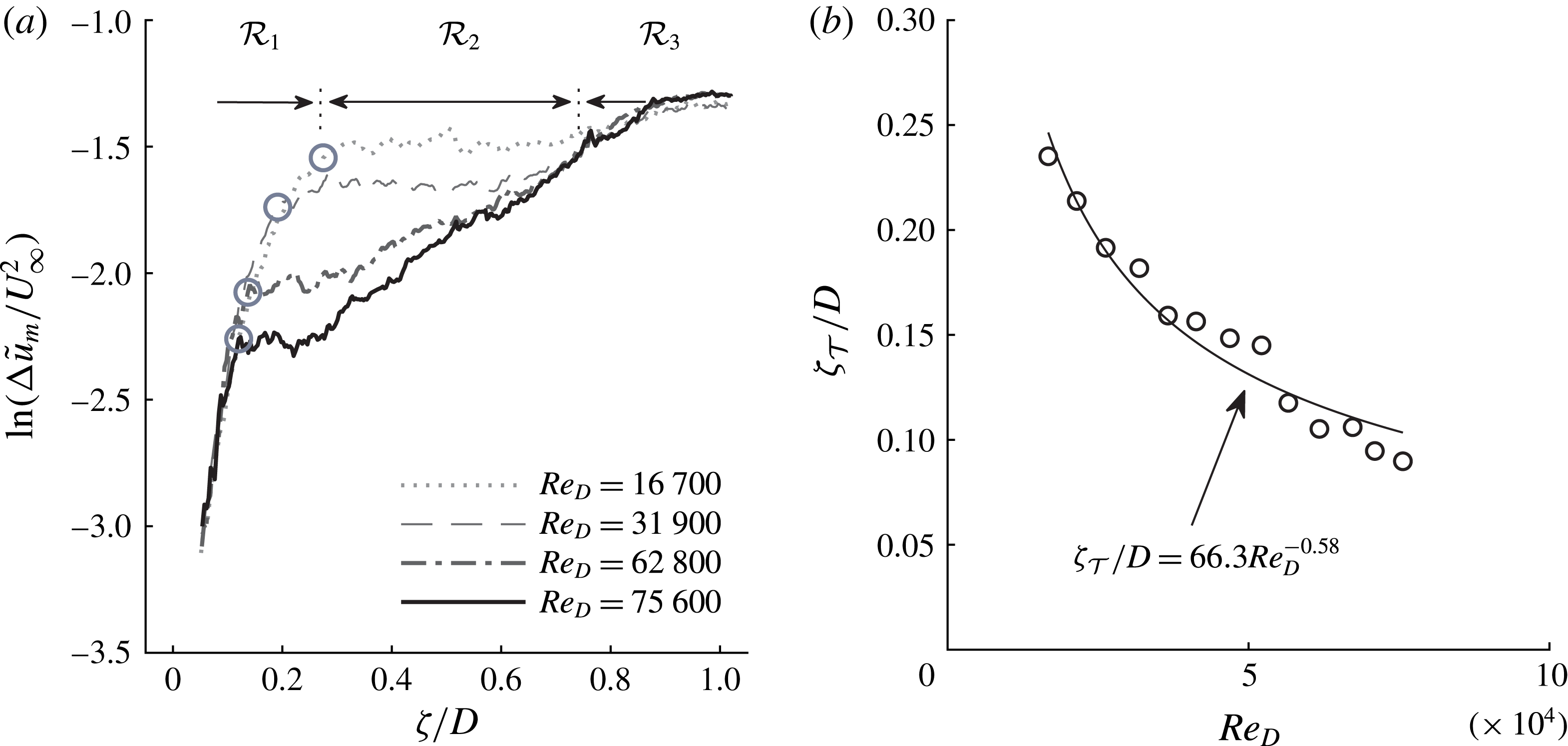
(a) Development of maximum fluctuations in shear layer,
 $\text{ln}(\unicode[STIX]{x0394}\tilde{u} _{m}/U_{\infty }^{2})$
, as a function of
 $\unicode[STIX]{x1D701}/D$
; (b) the transition point,
 $\unicode[STIX]{x1D701}_{{\mathcal{T}}}/D$
, defined at the end of the region of exponential KH growth, as a function of
 $Re_{D}$
.

3.4 Development of fluctuating quantities
In this section, parameters derived from the time-averaged fluctuations in the shear layer are examined and discussed. Figure 13(a) presents the development of the maximum fluctuation, defined as
 $$\begin{eqnarray}\displaystyle \tilde{u} _{m}={\textstyle \frac{1}{2}}(\overline{u^{2}}+\overline{v^{2}})_{max}. & & \displaystyle\end{eqnarray}$$
The parameter is presented along the arclength as a difference from the maximum fluctuation at separation,
 $\unicode[STIX]{x0394}\tilde{u} _{m}=\tilde{u} _{m}-\tilde{u} _{m,sep}$
, for several
 $Re_{D}$
. Considering
 $Re_{D}=16\,700$
, the development of
 $\unicode[STIX]{x0394}\tilde{u} _{m}$
exhibits three distinct regions: the first,
 ${\mathcal{R}}_{1}$
, is an initial region of exponential growth; the second,
 ${\mathcal{R}}_{2}$
, a plateau region with constant
 $\unicode[STIX]{x0394}\tilde{u} _{m}$
; and the third,
 ${\mathcal{R}}_{3}$
, exhibits a subsequent increase in the maximum fluctuation level. Regions
 ${\mathcal{R}}_{1}$
and
 ${\mathcal{R}}_{3}$
represent the growth of the KH and VK instabilities, respectively. In the laminar region, the KH instability waves grow exponentially in space, according to local linear stability theory (Michalke Reference Michalke1965). The VK instability on the other hand is absolute and affects all regions of the flow (Monkewitz & Nguyen Reference Monkewitz and Nguyen1987). The influence of the VK absolute instability manifests as a lateral flapping motion of the shear layer. The flapping, which increases in amplitude with distance from separation, is responsible for increased
 $\unicode[STIX]{x0394}\tilde{u} _{m}$
in
 ${\mathcal{R}}_{3}$
. The intermediate region,
 ${\mathcal{R}}_{2}$
, commences when the exponential growth of the KH instability saturates. The relative composition of the three regions exhibits strong
 $Re_{D}$
dependence. With increasing
 $Re_{D}$
, the junction between
 ${\mathcal{R}}_{1}$
and
 ${\mathcal{R}}_{2}$
moves upstream towards separation; similarly,
 ${\mathcal{R}}_{2}$
follows this migration while also decreasing in breadth. Region
 ${\mathcal{R}}_{3}$
thereby also moves upstream with
 $Re_{D}$
and contains increasing proportions of the shear layer region. Careful observation of the instantaneous PIV fields reveals that
 ${\mathcal{R}}_{2}$
initiates close to where the first KH vortex matures; that is, where the instability has saturated at a local maximum energy.
While the
 ${\mathcal{R}}_{1}$
–
 ${\mathcal{R}}_{2}$
junction displays
 $Re_{D}$
dependence, the spatial amplification rate of the KH instability is ostensibly constant. A spatial amplification factor or the slope of
 $\unicode[STIX]{x0394}\tilde{u} _{m}$
in
 ${\mathcal{R}}_{1}$
can be defined as
 $\unicode[STIX]{x1D70E}_{KH}=\text{ln}((\unicode[STIX]{x0394}\tilde{u} _{m}/U_{\infty }^{2})/(\unicode[STIX]{x1D701}/D))$
. It was found that
 $\unicode[STIX]{x1D70E}_{KH}=11.7$
, on average, for all Reynolds numbers tested. Some slight differences between
 $Re_{D}$
cases were observed; however, no trend could be discerned in particular. The PIV data capture the contribution of all disturbances, not just those at the most amplified frequency. It is thereby not possible to directly compare the magnitude of
 $\unicode[STIX]{x1D70E}_{KH}$
to the amplification rate of the most amplified frequency predicted by stability theory. The maximum growth rate of the KH instability in the plane mixing layer is approximately proportional to the velocity ratio,
 $R$
(Monkewitz Reference Monkewitz1982). As presented in figure 9(c),
 $R$
was a weak function of
 $Re_{D}$
over the range considered, and therefore one expects approximately constant
 $\unicode[STIX]{x1D70E}_{KH}$
.
Sato (Reference Sato1956) emphasised the gradual evolution from laminar to turbulent flow in the shear layer transition process, and that there are many ways for locating a ‘transition point’ within this region. The transition point should characterise a streamwise location which is consistent in the transition process. For Sato, this was where a sudden increase in the integrated fluctuating velocity was observed in a laminar boundary layer separating from a half-jet. Presumably, this was the initial inception of the KH instability. For the half-jet, the boundary layer momentum thickness at separation,
 $\unicode[STIX]{x1D703}_{sep}$
, could be determined from the Blasius solution and therefore it was found that the transition length was between
 $45\,\unicode[STIX]{x1D703}_{sep}$
and
 $52\,\unicode[STIX]{x1D703}_{sep}$
. Figure 13(a) demonstrates that the
 ${\mathcal{R}}_{1}$
–
 ${\mathcal{R}}_{2}$
junction is an easily distinguishable point along
 $\unicode[STIX]{x1D701}/D$
and is responsive to the influence of
 $Re_{D}$
. Thus the arclength from separation to the
 ${\mathcal{R}}_{1}$
–
 ${\mathcal{R}}_{2}$
junction is defined as a transition point,
 $\unicode[STIX]{x1D701}_{{\mathcal{T}}}$
, scaling with Reynolds number according to
 $$\begin{eqnarray}\displaystyle \frac{\unicode[STIX]{x1D701}_{{\mathcal{T}}}}{D}=\frac{66.3}{Re_{D}^{0.58}}, & & \displaystyle\end{eqnarray}$$
as presented in figure 13(b). This transition point will be revisited in the subsequent section where a length–velocity scaling argument is presented based on the PIV data.
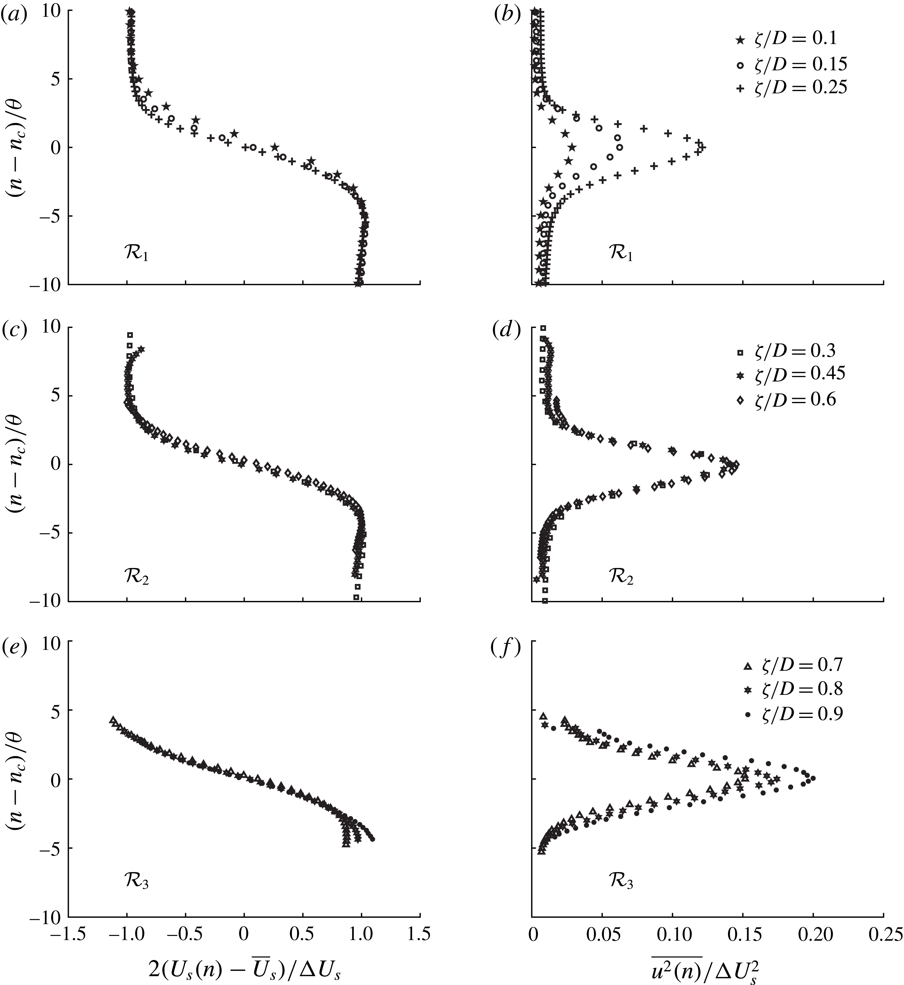
Distributions of local tangential velocity
 $2(U_{s}(n)-\overline{U}_{s})/\unicode[STIX]{x0394}U_{s}$
and local streamwise Reynolds stress,
 $\overline{u_{s}^{2}(n)}/\unicode[STIX]{x0394}U_{s}^{2}$
, presented in self-similar coordinates for
 $Re_{D}=16\,700$
for the three distinct regions identified in figure 13(a): (a,b)
 ${\mathcal{R}}_{1}$
; (c,d)
 ${\mathcal{R}}_{2}$
; and (e,f)
 ${\mathcal{R}}_{3}$
.

Figure 14 presents distributions of velocity and streamwise Reynolds stress in self-similar coordinates for
 $Re_{D}=16\,700$
, for the three distinct regions identified in figure 13(a). Figure 14(a,b) presents the local tangential velocity,
 $2(U_{s}(n)-\overline{U}_{s})/\unicode[STIX]{x0394}U_{s}$
and the local streamwise Reynolds stress,
 $\overline{u_{s}^{2}(n)}/\unicode[STIX]{x0394}U_{s}^{2}$
, respectively, along the normalised local axis,
 $(n-n_{c})/\unicode[STIX]{x1D703}$
, for the region
 ${\mathcal{R}}_{1}$
. It is clear that the data do not collapse in the self-similar coordinates; rather, this region is dominated by the growth of the KH instability and hence one should not expect a local equilibrium. Rather, with increasing
 $\unicode[STIX]{x1D701}/D$
,
 $\overline{u_{s}^{2}(n)}/\unicode[STIX]{x0394}U_{s}^{2}$
increases in magnitude as the KH instability amplifies. In region
 ${\mathcal{R}}_{2}$
, presented in figure 14(c,d), the data exhibit self-similarity in both profiles of velocity and turbulent stresses across the span of
 $\unicode[STIX]{x1D701}/D$
. Recall that
 ${\mathcal{R}}_{2}$
initiates close to where the first KH vortex matures; at this location, the instability has saturated and will begin to break down into random turbulence. It is apparent that, within this region, the shear layer maintains a local equilibrium demonstrated by the neat collapse in the self-similar coordinate system. In
 ${\mathcal{R}}_{3}$
, again the distributions of
 $\overline{u_{s}^{2}(n)}/\unicode[STIX]{x0394}U_{s}^{2}$
deviate from one another in the similarity coordinates. In this case it is the increasing influence of the wake flapping the shear layer that disrupts the equilibrium. Lyn & Rodi (Reference Lyn and Rodi1994) presented the mean and fluctuating quantities of the square-prism shear layer at
 $Re_{D}=21\,400$
in self-similar coordinates between
 $0.25\leqslant x/D\leqslant 1$
and found a reasonable collapse, although the collapse was less good between
 $0.75\leqslant x/D\leqslant 1$
, possibly indicating the influence of the wake. For
 $Re_{D}=21\,400$
, a profile taken at
 $x/D=0.25$
is very near the beginning of region
 ${\mathcal{R}}_{2}$
and therefore one would expect similarity to be observed. Furthermore, the study of Lyn & Rodi (Reference Lyn and Rodi1994) had free-stream turbulence of 2 %, which would have also altered the transition characteristics of the shear layer.
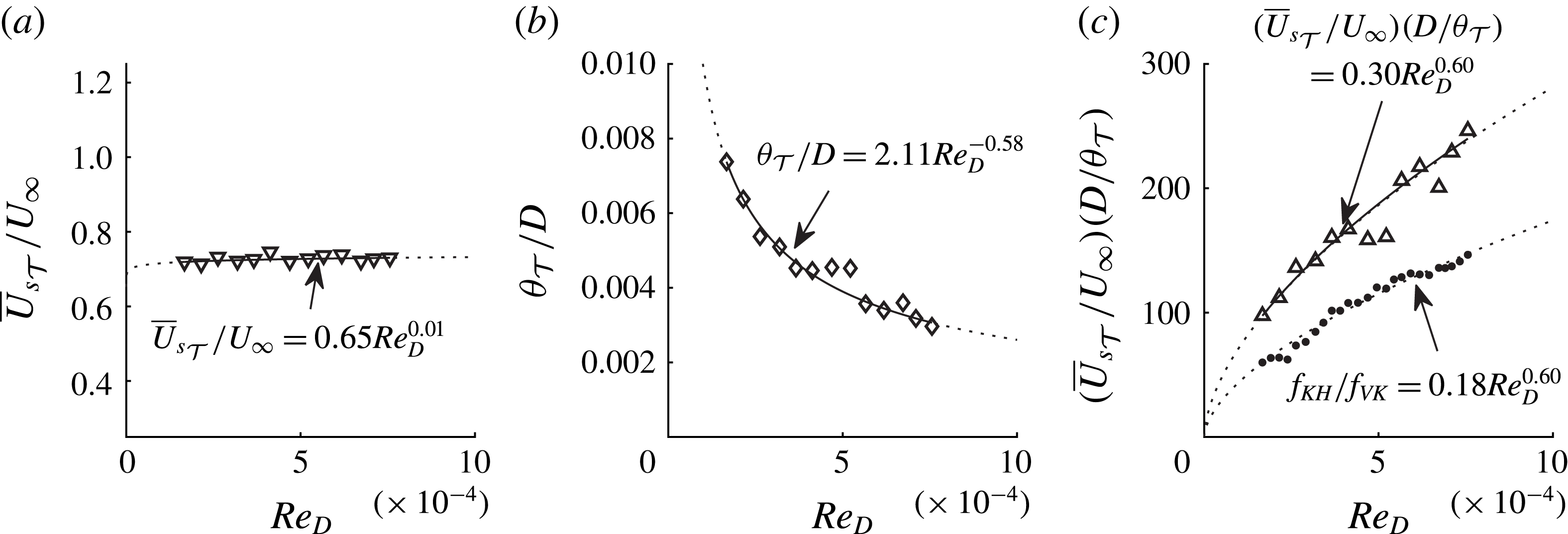
Shear layer scaling parameters evaluated at the transition point,
 $\unicode[STIX]{x1D701}_{{\mathcal{T}}}/D$
: (a) the velocity ratio
 $\overline{U}_{s_{{\mathcal{T}}}}/U_{\infty }$
; (b) the length ratio
 $\unicode[STIX]{x1D703}_{{\mathcal{T}}}/D$
; and (c) the combined length–velocity scaling with the frequency ratio scaling of (3.1), as a function of
 $Re_{D}$
.

3.5 Length–velocity scaling of the prism shear layer
The magnitude of the power in (3.8) is close to the power that appears in the frequency ratio scaling of (3.1). Indeed, this transition point, which moves upstream like
 $1/(Re_{D})^{0.58}$
, provides a suitable point to evaluate the length and velocity scales of the KH instability for the square prism from the PIV measurements. As discussed in § 1, Prasad & Williamson (Reference Prasad and Williamson1997) identified the influence of
 $Re_{D}$
on both the distance to transition and the width of the shear layer itself. Figure 10 demonstrates the influence of
 $Re_{D}$
on
 $\unicode[STIX]{x1D703}$
. The length and velocity scales of the KH instability are therefore the momentum thickness and the local average velocity across the shear layer, as commonly used in stability formulations (Michalke Reference Michalke1965), that is,
 $\unicode[STIX]{x1D703}$
and
 $\overline{U}_{s}$
evaluated at the transition point,
 $\unicode[STIX]{x1D701}_{{\mathcal{T}}}$
. Figure 15(a) presents the ratio
 $\overline{U}_{s_{{\mathcal{T}}}}/U_{\infty }$
, where a power-law best-fit follows the scaling
 $$\begin{eqnarray}\displaystyle \frac{\overline{U}_{s_{{\mathcal{T}}}}}{U_{\infty }}=0.65\,Re_{D}^{0.01}. & & \displaystyle\end{eqnarray}$$
Here, the velocity parameter of the KH instability is weakly dependent on
 $Re_{D}$
and the use of
 $U_{VK}=U_{\infty }$
in (3.6) was justified. Figure 15(b) presents
 $\unicode[STIX]{x1D703}_{{\mathcal{T}}}/D$
where the data follow the relation
 $$\begin{eqnarray}\displaystyle \frac{\unicode[STIX]{x1D703}_{{\mathcal{T}}}}{D}=2.11\,Re_{D}^{-0.58}. & & \displaystyle\end{eqnarray}$$
Finally, figure 15(c) compares the combined length–velocity scaling, which takes the form
 $$\begin{eqnarray}\displaystyle \frac{\overline{U}_{s_{{\mathcal{T}}}}}{U_{\infty }}\frac{D}{\unicode[STIX]{x1D703}_{{\mathcal{T}}}}=0.30\,Re_{D}^{0.60}, & & \displaystyle\end{eqnarray}$$
with the frequency ratio scaling of (3.1). The agreement between these scaling arguments is exceptional, with only a constant term,
 $C=0.60$
, separating a complete collapse of the scaling relationships.
3.6 Scaling at high
 $Re_{D}$

In the preceding sections, frequency ratio scaling of laminar KH vortices forming in the shear layer has been explored. With increasing
 $Re_{D}$
, the distance to the transition point moves upstream, the instability frequency increases and the size of KH vortices decreases. Using the hot-wire system, it was only possible to report the frequency characteristics of the KH instability up to
 $Re_{D}\simeq 75\,000$
. At higher
 $Re_{D}$
the spectral distributions at the KH frequency became difficult to discern from other high-frequency content. Nonetheless, the KH instability continues to form at smaller and smaller scales with increasing
 $Re_{D}$
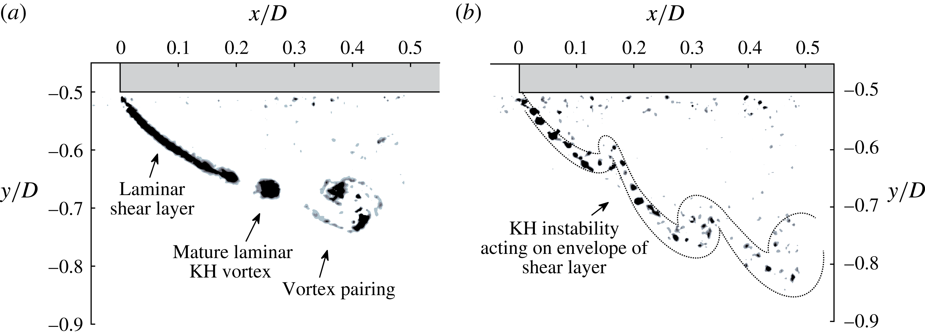
. In figure 16(a,b) a comparison is presented between two instantaneous renderings of Q criterion, at
 $Re_{D}=16\,700$
and
 $Re_{D}=101\,000$
, respectively. In both cases, the laminar vortices are visible; however, the high-
 $Re_{D}$
vortices are much smaller and mature closer to the leading edge.
Instantaneous Q criterion presented for
 $Re_{D}=16\,700$
and 101 000 illustrating the (a) low-
 $Re_{D}$
and (b) high-
 $Re_{D}$
comparison of the KH instability for the square-prism shear layer.

In figure 16(b) a secondary effect is also observable. Downstream of separation, an apparent clustering of the small laminar vortices is present. An outline of the clustered vortices has been added for clarity. Brown & Roshko (Reference Brown and Roshko1974) famously identified turbulent coherent structures in plane mixing layers at very large Reynolds number where the KH instability re-emerged by folding the ‘envelope’ of the region of shear. The high-Reynolds-number manifestation of the KH instability requires a sizeable disparity between the large (outer) and small (inner) scales of turbulence, according to Liu & Merkine (Reference Liu and Merkine1976), in which case it is essentially governed by the same dynamic processes as the laminar formation (Ho & Huerre Reference Ho and Huerre1984). The re-emergence of the KH instability is mentioned here as a final thought to note that an upper
 $Re_{D}$
limit may exist where the scaling argument presented herein remains relevant. That is, above a certain
 $Re_{D}$
, the frequency ratio scaling of the laminar vortices will be superseded by lower-frequency KH instability which acts on the time-averaged shear generated by fine-scale turbulent fluctuations. Nonetheless, if the stability considerations of Sigurdson (Reference Sigurdson1986) are accurate and valid for the square prism, the front-face boundary layer remains laminar until
 $Re_{\unicode[STIX]{x1D6FF}}\simeq 10^{9}$
. Hence, smaller and smaller laminar vortices will continue to form as the front-face boundary layer continues to thin.
4 Summary and conclusions
In this investigation, the mechanisms of transition in the shear layers of a square prism were observed and interpreted with respect to the documented frequency ratio,
 $f_{KH}/f_{VK}$
, as it changed with
 $Re_{D}$
. For the square prism, the ratio between the shear layer frequency and the shedding frequency followed a power-law scaling argument of the form
 $$\begin{eqnarray}\displaystyle \frac{f_{KH}}{f_{VK}}=0.18\,Re_{D}^{0.60}. & & \displaystyle\end{eqnarray}$$
The adherence to this relationship, which was derived from hot-wire measurements, has been supported by two additional and independent scaling considerations: namely, by PIV to observe the evolution of length and velocity scales in the shear layer during transition, and by DNS to illuminate the properties of the front-face boundary layer. A key finding of this investigation is that the nonlinear Reynolds-number dependence of the frequency ratio scaling is driven by the sustained influence on the thickness of the laminar front-face boundary layer.
We note that the original scaling argument proposed by Bloor (Reference Bloor1964) relied solely on the length scale of the shear layer as the source of the nonlinearity of
 $f_{KH}/f_{VK}$
with
 $Re_{D}$
. The subsequent investigation of Prasad & Williamson (Reference Prasad and Williamson1997) demonstrated the need also to consider the influence of
 $Re_{D}$
on shear transition and shedding frequency for the circular cylinder. For the square prism,
 $St_{D}$
is unchanging over a large range of
 $Re_{D}$
, and therefore the power-law scaling of
 $f_{KH}/f_{VK}$
may be understood by the influence of
 $Re_{D}$
on the appropriate length scale of the shear layer. In this study it was found that the momentum thickness evaluated at a transition point, defined where the KH instability saturates, exhibits the same
 $Re_{D}$
dependence as the frequency ratio.
Acknowledgements
The authors wish to acknowledge the support of Dr K. Taylor, Dr C. M. Leong and Mr D. Digiulio. We also wish to express our gratitude to Professor C. Vassilicos, Dr G. Papadakis, Dr F. A. Portela, Dr F. X. Trias, Dr A. Gorobets and Dr A. Oliva for generously providing the direct numerical simulation data used in this study. Financial support was provided by the National Science Foundation under grant NSF CMMI-1200987.