1. Introduction and context
Although the dynamics of a cylinder wake is well-known for a homogeneous fluid, there are very few studies for a stratified fluid. This paper analyses the transition from a two-dimensional (2D) von Kármán street to three-dimensional (3D) instabilities in a stratified cylinder wake, based on experimental evidence and with some numerical clues about the structures observed.
Bluff body wakes have been a main subject of interest for engineers due to their applications to terrestrial and naval vehicles as well as to civil constructions, where the presence of alternated vortices in the wakes may cause structural vibrations leading to catastrophic failures. However a simple geometry like a circular cylinder presents all the main characteristics of bluff body wakes which is why this basic geometry is often used for fundamental studies on bluff body wakes.
The 2D dynamics of a cylinder wake has been greatly studied in the last century. At low Reynolds number the flow is stationary and is characterized by a steady recirculation bubble behind the cylinder but a 2D periodic structure appears for
 $\mathit{Re}\geqslant 50$
with the presence of alternate vortices (see Williamson Reference Williamson1996a
, for a review).
For higher Reynolds number, the dynamics of the cylinder wake is strongly modified due to the appearance of three-dimensional instabilities. The first unstable mode, called mode A, has been observed experimentally (Hama Reference Hama1957; Bloor Reference Bloor1964; Norberg Reference Norberg1994; Zhang et al.
Reference Zhang, Fey, Noack, Konig and Eckelmann1995; Williamson Reference Williamson1996b
, Reference Williamson1988) and also by direct numerical simulations (DNS) (Karniadakis & Triantafyllou Reference Karniadakis and Triantafyllou1992; Thompson, Hourigan & Sheridan Reference Thompson, Hourigan and Sheridan1994, Reference Thompson, Hourigan and Sheridan1996; Zhang et al.
Reference Zhang, Fey, Noack, Konig and Eckelmann1995; Henderson Reference Henderson1997). The critical Reynolds number at which the mode becomes unstable varies between 150 and 190 (Williamson Reference Williamson1988; Karniadakis & Triantafyllou Reference Karniadakis and Triantafyllou1992; Zhang et al.
Reference Zhang, Fey, Noack, Konig and Eckelmann1995; Williamson Reference Williamson1996a
). This large range is probably due to oblique shedding in the experiments and due to the fact that the transition is slightly subcritical (Henderson Reference Henderson1997; Behara & Mittal Reference Behara and Mittal2010). However, Barkley (Reference Barkley1996) showed by a Floquet analysis that the mode A becomes linearly unstable at a critical Reynolds number
 $\mathit{Re}=188.5\pm 1.0$
at a spanwise wavelength equal to
 $3.96\pm 0.02$
diameters. This is in excellent agreement with the experiments and the DNS. The mode A seems to be the result of an elliptic instability of the von Kármán vortices, as claimed by Williamson (Reference Williamson1996b
), Leweke & Williamson (Reference Leweke and Williamson1998) and Thompson, Leweke & Williamson (Reference Thompson, Leweke and Williamson2001), since it gives correct predictions of the spatial structure and of the wavelength.
At a Reynolds number larger than 230, a new unstable mode, called mode B, emerges with smaller-scale irregular patterns (Williamson Reference Williamson1988; Zhang et al.
Reference Zhang, Fey, Noack, Konig and Eckelmann1995; Henderson Reference Henderson1997). This mode is also predicted by the Floquet analysis of Barkley (Reference Barkley1996) at a critical Reynolds number equal to 259 and a wavelength equal to 0.82 diameters. Wu et al. (Reference Wu, Sheridan, Welsh and Hourigan1996) showed experimentally that this mode contains strong longitudinal vortices. This suggests that this mode B is due to the stretching of vorticity by the stagnation points of the two-dimensional base flow located between two von Kármán vortices, as in the case of the wake of a flat plate (Meiburg & Lasheras Reference Meiburg and Lasheras1988). Modes A and B have a different symmetry: the longitudinal vortices rotate in the same direction at each half-wavelength for mode B, whereas they rotate in opposite directions at each half-wavelength for mode A (Williamson Reference Williamson1996a
). The bifurcation due to the unstable mode B is supercritical (Henderson Reference Henderson1997). Mode B is present together with mode A up to
 $\mathit{Re}=260$
. Above this Reynolds number, the mode B becomes dominant. This coexistence of two modes can be modelled theoretically by two coupled nonlinear Landau equations (Barkley, Tuckerman & Golubitski Reference Barkley, Tuckerman and Golubitski2000), which allow prediction of the Strouhal number as a function of the Reynolds number (Sheard, Thompson & Hourigan Reference Sheard, Thompson and Hourigan2003).
Although the homogeneous dynamics of a cylinder wake has been extensively studied, very few papers have focused on stratified wakes despite obvious applications to geophysical flows and submarine wakes. Given that oceans and the atmosphere are stratified, most environmental flows like island wakes and mountain range wakes are strongly influenced by the mean density gradient. Also, the stable oceanic stratification is a key ingredient in naval applications such as submarine wakes. This interest has resulted in laboratory investigations of the turbulent regime of a bluff body with a finite height like a sphere, a spheroid or a streamwise cylinder at large Reynolds number. The early paper of Lin & Pao (Reference Lin and Pao1979) showed that the isotropic wake becomes quasi-2D with a saturation of the height after a time inversely proportional to the Brunt–Väisälä frequency
 $N$
. Large horizontal vortices with limited vertical scale are created. They grow in width by merging together which gives rise to an algebraic growth of the wake width and an algebraic decay of the velocity. The scaling laws for the width and the velocity have been established for a sphere by Spedding (Reference Spedding1997) and extended to different geometries by Meunier & Spedding (Reference Meunier and Spedding2004). The exponents were recovered theoretically by Meunier & Spedding (Reference Meunier and Spedding2006) who assumed that the Reynolds stress is proportional to the mean shear. Diamessis, Spedding & Domaradzki (Reference Diamessis, Spedding and Domaradzki2011) finally showed that at large Reynolds number, Kelvin–Helmholtz billows are created at the top and the bottom of the horizontal vortices. It was shown by Brucker & Sarkar (Reference Brucker and Sarkar2010) that the wake of a self-propelled body decays faster in the early stages but slower in the late stages, as observed experimentally by Meunier & Spedding (Reference Meunier and Spedding2006). However, in practice, the presence of a small acceleration introduces some momentum which governs the dynamics of the wake (Meunier & Spedding Reference Meunier and Spedding2006).
Stratified wakes of a horizontal cross-stream cylinder have received even less attention. Boyer et al. (Reference Boyer, Davies, Fernando and Zhang1989) discovered a large variety of regimes when the Froude number varies from 0.02 to 13 and the Reynolds number varies from 5 to 4000. For strong stratification, they revealed the presence of internal waves, of an accelerated flow on the centreline and of isolated recirculation bubbles downstream of the cylinder. The flow also creates a recirculating bubble upstream of the cylinder, which is known as the blocking effect, studied by Browand & Winant (Reference Browand and Winant1972), Baines (Reference Baines1987), Xu, Fernando & Boyer (Reference Xu, Fernando and Boyer1995) and Winters & Armi (Reference Winters and Armi2012). When the Reynolds number increases, Boyer et al. (Reference Boyer, Davies, Fernando and Zhang1989) showed that the flow transitions to vortex shedding and to a turbulent flow. But the stratification tends to prevent the appearance of von Kármán vortices, due to the stabilization of shear flows by a stratification. This effect can be quantified by the Richardson criterion, leading to the dependence of the critical Reynolds number on the Froude number (Meunier Reference Meunier2012a ).
However, the dynamics of the wake is strongly modified when the cylinder is no longer horizontal but tilted with respect to the vertical. Meunier (Reference Meunier2012a ) showed experimentally and numerically that von Kármán vortices can be emitted for strong stratifications at moderate Reynolds numbers. This is in agreement with the new unstable mode found by Candelier, Le Dizès & Millet (Reference Candelier, Le Dizès and Millet2011) in a tilted jet using a linear stability analysis. The existence of tilted vortices in a strongly stratified fluid is made possible because the streamlines remain horizontal but centred around a tilted axis (Boulanger, Meunier & Le Dizès Reference Boulanger, Meunier and Le Dizès2006; Canals, Pawlak & MacCready Reference Canals, Pawlak and MacCready2009). However, this structure generates a critical layer at the radius where the angular velocity equals the Brunt–Väisälä frequency, leading to strong axial shears which are unstable with respect to the Kelvin–Helmholtz instability (Boulanger, Meunier & Le Dizès Reference Boulanger, Meunier and Le Dizès2007).
To conclude, the 3D instabilities of a stratified cylinder wake have been only briefly studied. Moreover, they focused on the case of a horizontal cylinder despite the strong influence of the tilt angle. The goal of this paper is thus to characterize this transition experimentally for all tilt angles and Froude numbers.
The paper is organized as follows. In § 2, we describe the experimental set-up and the reduced governing equations. Section 3 is devoted to the mode A, well-known in the case of a homogeneous fluid, for a nearly vertical cylinder. Section 4 presents another instability mode appearing for a moderate tilt angle. The case of a nearly horizontal cylinder is finally treated, for a weak stratification (§ 5) and for a strong stratification (§ 6). Conclusions follow in § 7.
2. Materials and methods
2.1. Experimental details
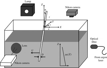
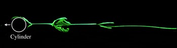
The model experiment used to study the dynamics of a stratified cylinder wake is presented schematically in figure 1. A 150 cm long, 75 cm wide and 50 cm high Plexiglas tank is built in order to make visualizations from all sides.
Schematic of the experimental set-up: the stratified cylinder wake is analysed by dye visualizations on the right-hand side and by the shadowgraph method on the left-hand side.

The tank contains a stable linearly salt-stratified fluid up to a water height
 $H=40\ \text{cm}$
obtained by the double bucket method (see Fortuin Reference Fortuin1960). The water from the first bucket (filled with salted water at a density
 ${\it\rho}=1.15\ \text{kg}\ \text{l}^{-1}$
) is slowly deposited at the surface of the tank using a floater. The density of the first bucket is gradually decreased by the addition of fresh water from a second bucket. The density gradient is obtained from density measurements of small samples of fluid every 10 cm, using a densitometer Anton Paar DMA 35N with an accuracy of
 $10^{-4}\ \text{kg}\ \text{l}^{-1}$
. The typical Brunt–Väisälä frequency defined by
 $N\simeq \sqrt{(-g/{\it\rho}_{0})(\text{d}\bar{{\it\rho}}/\text{d}Z)}$
is close to
 $2\ \text{rad}\ \text{s}^{-1}$
(with
 ${\it\rho}_{0}$
the mean density in the tank and
 $\bar{{\it\rho}}$
is the mean density profile
 $\bar{{\it\rho}}(z)$
). The stratification can stay linear for approximately two months except at the top and the bottom of the tank because of mixing at the extreme layers. Fresh water is deposited weekly at the free layer so as to reduce the evaporation effect.
To study the dynamics, a circular cylinder of diameter
 $D$
is introduced in the tank. This cylinder is towed horizontally in the stratified fluid, at a velocity
 $U$
varying between 0.5 and
 $5\ \text{cm}\ \text{s}^{-1}$
. The diameter varies between 0.3 and 1.8 cm. The cylinder can be tilted relative to the vertical, at an angle
 ${\it\alpha}$
in the cross-stream plane as can be seen on figure 1. The cylinder is mounted on a carriage that moves along horizontal rails, pulled by a belt driven by a DC motor coupled to a 1:90 reducer. The towing velocity is stable within 0.1 % even at low speed.
As shown on figure 1, two visualization methods are used. The first one is the shadowgraph method which reveals non-uniformities in the water tank. On one side of the tank, a light is placed far from the tank in order to create parallel light which goes through the test section and whose rays are deviated by refraction. A lens and a camera located at the focal distance are placed at the opposite side of the tank. The deviated rays do not enter the camera, creating dark areas on the images, which thus reveal the density gradients. The other visualization method consists of depositing a fluorescent dye mixture made of Fluorescein and silicon on the upstream side of the cylinder. Once the dye is dry, the cylinder is slowly lowered into the water without disturbing the fluid. During the experiment, the dye is advected by the flow and detaches at the separation point together with the vorticity. These methods are used to determine the stability of the flow and to measure the wavelength and recirculation length of the wake.
The stratified wake of the tilted cylinder is characterized by four non-dimensional parameters: the cross-stream tilt angle
 ${\it\alpha}$
, the Reynolds number
 $\mathit{Re}$
, the Froude number
 $F$
and the Schmidt number
 $\mathit{Sc}$
. However, the last parameter defined as
 $\mathit{Sc}={\it\nu}/{\it\kappa}=700$
(
 ${\it\kappa}$
being the diffusivity of salt in water) is large in this study, which reduces the problem to three main non-dimensional parameters.
The tilt angle
 ${\it\alpha}$
varies between 0 and 90°. When the cylinder is nearly vertical, the support mechanism for the cylinder is not submerged in the tank. For nearly horizontal cylinders, the cylinder has two thin vertical plates fixed on both ends which are profiled in order to prevent perturbations. The Reynolds number
 $\mathit{Re}=UD/{\it\nu}$
is varied between 30 and 300. In our experiments, the kinematic viscosity
 ${\it\nu}$
increases by 10 % from the top to the bottom due to the presence of salt, which introduces an error in the Reynolds number of 5 %. There is no temperature variation with the depth but the temperature was measured within half a degree in order to be accurate within 2 % for the mean Reynolds number. The Froude number
 $F=U/ND$
, is varied between 0.5 and 8 by changing the diameter
 $D$
and the velocity of the cylinder simultaneously. The stratification length
 $L$
defined by
 $L={\it\rho}_{0}H/(\text{d}\bar{{\it\rho}}/\text{d}z)$
quantifies the non-Boussinesq effects, which are proportional to
 $1/L$
. Since
 $L$
is very large in our experiments (
 $L\simeq 300$
), the whole study is thus done under the Boussinesq approximation.
Use of a channel is essential for stratified fluids. However, the dimensionless wavelength is independent of the towing distance, corresponding to the distance between the lens and the location where the cylinder begins to be towed, but for all the experiment points, the cylinder was in a steady regime. An uncertainty can be noted of the order of 10 % from the data where the towing distance was varied.
2.2. Numerical formulation of the problem
The flow is governed by the Navier–Stokes equations coupled with the density equation and the incompressibility condition:
 $$\begin{eqnarray}\displaystyle & \displaystyle \frac{\text{D}\boldsymbol{u}}{\text{D}t}=-\frac{1}{{\it\rho}_{0}}\boldsymbol{{\rm\nabla}}p+\frac{{\it\rho}}{{\it\rho}_{0}}\boldsymbol{g}+{\it\nu}{\rm\Delta}\boldsymbol{u}, & \displaystyle\end{eqnarray}$$
 $$\begin{eqnarray}\displaystyle & \displaystyle \frac{\text{D}(\bar{{\it\rho}}+{\it\rho})}{\text{D}t}={\it\kappa}{\rm\Delta}{\it\rho}, & \displaystyle\end{eqnarray}$$
 $$\begin{eqnarray}\displaystyle & \displaystyle \boldsymbol{{\rm\nabla}}\boldsymbol{\cdot }\boldsymbol{u}=0. & \displaystyle\end{eqnarray}$$
These equations are written in the Boussinesq approximation where the density perturbation
 ${\it\rho}$
and the mean density profile
 $\bar{{\it\rho}}(Z)$
are smaller than the absolute density
 ${\it\rho}_{0}$
and where the static pressure is removed. The problem is solved in the frame of reference moving with the cylinder. The translation of the fluid is thus imposed by the boundary conditions at infinity:
 $u=U$
and
 $v=w={\it\rho}=0$
. At the surface of the cylinder (
 $r=D/2$
), no-slip boundary conditions are imposed for the velocity (
 $u=v=w=0$
) and the normal flux of density is taken equal to zero (
 $\partial {\it\rho}/\partial n=0$
). The towing velocity
 $U$
, the cylinder diameter
 $D$
and the mean density
 ${\it\rho}_{0}$
are used to non-dimensionalize the problem. Thus lengths are non-dimensionalized by
 $D$
, times by
 $D/U$
and mass by
 ${\it\rho}_{0}D^{3}$
. The study is solved in the tilted frame of reference
 $(Oxyz)$
of the cylinder, whose axes are tilted by an angle
 ${\it\alpha}$
compared to the vertical/horizontal axes
 $(OXYZ)$
, as sketched on figure 1. The gravity
 $\boldsymbol{g}$
thus contains a
 $y$
and a
 $z$
component. Also the term
 $\text{D}\bar{{\it\rho}}/\text{D}t$
contains both the
 $y$
and
 $z$
component of the velocity. Thus in a first step, the 2D flow (i.e. invariant along the cylinder’s axis) is calculated corresponding to the base flow. The 2D flow is governed by five equations for the velocity
 $(u_{2\mathit{D}},v_{2\mathit{D}},w_{2\mathit{D}})$
, pressure
 $p_{2\mathit{D}}$
and density
 ${\it\rho}_{2\mathit{D}}$
depending on
 $x$
and
 $y$
only:
 $$\begin{eqnarray}\displaystyle & \displaystyle \frac{\tilde{\text{D}}u_{2\mathit{D}}}{\tilde{\text{D}}t}=-\frac{\partial p_{2\mathit{D}}}{\partial x}+\frac{1}{\mathit{Re}}{\rm\Delta}u_{2\mathit{D}}, & \displaystyle\end{eqnarray}$$
 $$\begin{eqnarray}\displaystyle & \displaystyle \frac{\tilde{\text{D}}v_{2\mathit{D}}}{\tilde{\text{D}}t}=-\frac{\partial p_{2\mathit{D}}}{\partial y}+\frac{{\it\rho}_{2\mathit{D}}\sin {\it\alpha}}{F^{2}}+\frac{1}{\mathit{Re}}{\rm\Delta}v_{2\mathit{D}}, & \displaystyle\end{eqnarray}$$
 $$\begin{eqnarray}\displaystyle & \displaystyle \frac{\tilde{\text{D}}w_{2\mathit{D}}}{\tilde{\text{D}}t}=-\frac{{\it\rho}_{2\mathit{D}}\cos {\it\alpha}}{F^{2}}+\frac{1}{\mathit{Re}}{\rm\Delta}w_{2\mathit{D}}, & \displaystyle\end{eqnarray}$$
 $$\begin{eqnarray}\displaystyle & \displaystyle \frac{\tilde{\text{D}}{\it\rho}_{2\mathit{D}}}{\tilde{\text{D}}t}=w_{2\mathit{D}}\cos {\it\alpha}-v_{2\mathit{D}}\sin {\it\alpha}+\frac{1}{\mathit{Re}\mathit{Sc}}{\rm\Delta}{\it\rho}_{2\mathit{D}}, & \displaystyle\end{eqnarray}$$
 $$\begin{eqnarray}\displaystyle & \displaystyle \frac{\partial u_{2\mathit{D}}}{\partial x}+\frac{\partial v_{2\mathit{D}}}{\partial y}=0. & \displaystyle\end{eqnarray}$$
In these equations, the density
 ${\it\rho}_{2\mathit{D}}$
has been further non-dimensionalized by the non-dimensional stratification length
 $L$
, and
 $\tilde{\text{D}}/\tilde{\text{D}}t=\partial /\partial t+u_{2\mathit{D}}\partial /\partial x+v_{2\mathit{D}}\partial /\partial y$
corresponds to the 2D Lagrangian derivative in the plane perpendicular to the cylinder. Since there is no advection term
 $w_{2\mathit{D}}\partial /\partial z$
for a 2D flow, the problem can be treated as a two-dimensional flow for
 $(u_{2\mathit{D}},v_{2\mathit{D}})$
depending on
 $x$
and
 $y$
only with two active scalars
 $w_{2\mathit{D}}$
and
 ${\it\rho}_{2\mathit{D}}$
. The forcing term in the second equation is considered as a volumic force and the forcing terms in the third and fourth equations are considered as creation rates of the scalars
 $w_{2\mathit{D}}$
and
 ${\it\rho}_{2\mathit{D}}$
. For a strongly stratified fluid, the fluid moves mostly in a horizontal plane which means that velocity
 $v_{2\mathit{D}}$
is compensated by
 $w_{2\mathit{D}}$
such that
 $w_{2\mathit{D}}\cos {\it\alpha}-v_{2\mathit{D}}\sin {\it\alpha}$
is close to 0.
In a second step, the 3D flow has been calculated in order to find the 3D unstable modes. The 3D flow is simply modelled as a sinusoidal perturbation of wavenumber
 $k$
added to the base flow:
 $$\begin{eqnarray}\left.\begin{array}{@{}l@{}}\displaystyle u(x,y,z,t)=u_{2\mathit{D}}(x,y,t)+u_{1}(x,y,t)\cos kz-u_{2}(x,y,t)\sin kz,\\ \displaystyle v(x,y,z,t)=v_{2\mathit{D}}(x,y,t)+v_{1}(x,y,t)\cos kz-v_{2}(x,y,t)\sin kz,\\ \displaystyle w(x,y,z,t)=w_{2\mathit{D}}(x,y,t)+w_{1}(x,y,t)\sin kz+w_{2}(x,y,t)\cos kz,\\ \displaystyle p(x,y,z,t)=p_{2\mathit{D}}(x,y,t)+p_{1}(x,y,t)\cos kz-p_{2}(x,y,t)\sin kz,\\ \displaystyle {\it\rho}(x,y,z,t)={\it\rho}_{2\mathit{D}}(x,y,t)+{\it\rho}_{1}(x,y,t)\sin kz+{\it\rho}_{2}(x,y,t)\cos kz.\end{array}\right\}\end{eqnarray}$$
It can be noted that in this 3D decomposition, time dependence is suppressed but the 2D basic state is possibly time dependent. This decomposition is then introduced in the Navier–Stokes equations (2.1) which are linearized for the 3D perturbations
 $\boldsymbol{u}_{1}$
and
 $\boldsymbol{u}_{2}$
. Separating the Fourier components leads to three systems of equations for the base flow and the two perturbations. The system of equations for the base flow is similar to the 2D case and is given by (2.2).
The equations governing the perturbation
 $(u_{1},v_{1},w_{1},p_{1},{\it\rho}_{1})$
can be written as follows:
 $$\begin{eqnarray}\displaystyle & \displaystyle \frac{\tilde{\text{D}}\boldsymbol{u}_{1}}{\tilde{\text{D}}t}+(\boldsymbol{u}_{1}\boldsymbol{\cdot }\tilde{\boldsymbol{{\rm\nabla}}})\tilde{\boldsymbol{u}}_{2\mathit{D}}+{\it\epsilon}_{1}[(\boldsymbol{u}_{2}\boldsymbol{\cdot }\tilde{\boldsymbol{{\rm\nabla}}})(w_{2\mathit{D}}\boldsymbol{e}_{z})-kw_{2\mathit{D}}\boldsymbol{u}_{2}] & \displaystyle \nonumber\\ \displaystyle & \quad =-(\tilde{\boldsymbol{{\rm\nabla}}}p_{1}-kp_{1}\boldsymbol{e}_{z})+\frac{\tilde{{\rm\Delta}}-k^{2}}{\mathit{Re}}\boldsymbol{u}_{1}+R_{1}, & \displaystyle\end{eqnarray}$$
 $$\begin{eqnarray}\displaystyle & \displaystyle \tilde{\boldsymbol{{\rm\nabla}}}\boldsymbol{\cdot }\boldsymbol{u}_{1}+kw_{1}=0, & \displaystyle\end{eqnarray}$$
 $$\begin{eqnarray}\displaystyle & \displaystyle \frac{\tilde{\text{D}}{\it\rho}_{1}}{\tilde{\text{D}}t}+{\it\epsilon}_{1}[kw_{2\mathit{D}}{\it\rho}_{2}-(\boldsymbol{u}_{2}\boldsymbol{\cdot }\tilde{\boldsymbol{{\rm\nabla}}}){\it\rho}_{2\mathit{D}}]=\frac{\tilde{{\rm\Delta}}-k^{2}}{\mathit{Re}\mathit{Sc}}{\it\rho}_{1}+w_{1}\cos {\it\alpha}+{\it\epsilon}_{1}v_{2}\sin {\it\alpha}. & \displaystyle\end{eqnarray}$$
Here
 $R_{1}=(0,{\it\epsilon}_{1}{\it\rho}_{2}\sin {\it\alpha},-{\it\rho}_{1}\cos {\it\alpha})/F^{2}$
corresponds to the buoyancy force,
 ${\it\epsilon}_{1}=1$
and
 $\boldsymbol{e}_{z}$
is the axial unit vector;
 $\tilde{\text{D}}/\tilde{\text{D}}t=\partial _{t}+\tilde{\boldsymbol{u}}_{2\mathit{D}}\boldsymbol{\cdot }\boldsymbol{{\rm\nabla}}$
corresponds to the 2D Lagrangian derivative with
 $\tilde{\boldsymbol{u}}_{2\mathit{D}}=(u_{2\mathit{D}},v_{2\mathit{D}},0)$
the cross-cut component of the base flow. We have also defined the 2D divergence
 $\tilde{\boldsymbol{{\rm\nabla}}}=(\partial _{x},\partial _{y},0)$
and the 2D Laplacian operator
 $\tilde{{\rm\Delta}}=\partial ^{2}/\partial x^{2}+\partial ^{2}/\partial y^{2}$
. The system of equations for the second perturbation
 $(u_{2},v_{2},w_{2},p_{2},{\it\rho}_{2})$
is simply obtained by inverting indices 1 and 2 with
 ${\it\epsilon}_{2}=-1$
.
Numerically, the problem is solved in a rectangle with
 $x\in [-4,16]$
and
 $y\in [-5,5]$
, the cylinder being centred at
 $(x=0,y=0.1)$
. The small
 $y$
-offset allows the symmetry of the numerical wake to be broken and thus prevents the solution locking on a stable wake. The boundary conditions on the outer rectangle are slightly different than in the theoretical problem. At the entrance of the flow (
 $x=-4$
), the velocity is imposed as
 $(u_{2\mathit{D}},v_{2\mathit{D}},w_{2\mathit{D}})=(1,0,0)$
and the density is equal to 0. On the side walls (
 $y=\pm 5$
), slip boundary conditions for the
 $(u,v)$
velocity are used and no outward flux of density and vertical velocity
 $w$
is imposed. At the exit of the flow (
 $x=16$
), the boundary is assumed to exert no force on the fluid (stress tensor equal to zero) and there is no diffusive flux of density and vertical velocity (
 $\partial {\it\rho}/\partial x=\partial w/\partial x=0$
). At the surface of the cylinder, the boundary conditions are taken as previously stated: no-slip boundary conditions for the velocity and no normal flux of density. Moreover the boundary conditions satisfied by the 3D perturbations
 $\boldsymbol{u}_{1}$
and
 $\boldsymbol{u}_{2}$
are similar to the base flow.
The study is solved using Comsol Multiphysics©, which is a finite element method allowing the coupling of several partial differential equations. The numerical study is initiated with the two-dimensional dynamics. Once the von Kármán wake is fully developed, we solve simultaneously the equations for the 3D perturbations. When the flow is unstable, the numerical noise is sufficient to give an exponential growth of the perturbation. The initial conditions can be taken either with zero initial flow or as the flow previously obtained at different parameters (higher or smaller Reynolds number for example). This allows the measurement of negative growth rates when the 3D perturbation decays exponentially. The number of degrees of freedom can be up to 376 700 noting that the mesh elements are solved with 15 unknown parameters. Quintic Lagrange elements are used for each variable. Some computations have been done for a Reynolds number
 $\mathit{Re}=120$
, a Froude number
 $F=4$
with
 ${\it\alpha}=0^{\circ }$
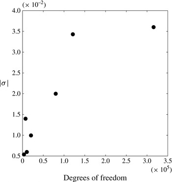
with different degrees of freedom by changing the accuracy of the mesh in the code. The results of absolute value of the instability growth rate are plotted in figure 2 for different degrees of freedom. The absolute value of the growth rate converges when the degree of freedom increases which gives confidence regarding the prediction of the critical Reynolds number for the mode A as the average degrees of freedom used is around 360 000.
Test of convergence of the absolute value of the instability growth rate for different degrees of freedom for a tilt angle
 ${\it\alpha}=0^{\circ }$
at
 $\mathit{Re}=120$
and
 $F=4$
.

The time-dependent simulations are solved by an iterative method generalized minimal residual (GMRES) algorithm which has the property of minimizing at every step the norm of the residual vector over a Krylov subspace derived from the Arnoldi process. The iterations are determined by a stopping rule based on the discrepancy principle. The simulations are carried out over a long time (up to
 $t=500$
in dimensionless units) to allow the von Kármán instability to grow and saturate. This could take up to 72 h of computation for one set of parameters on a Mac Book Pro.
3. Mode A: the instability of nearly vertical cylinders
In this section, we focus on the stability of the wake when the cylinder is vertical or weakly tilted.
3.1. Shadowgraph visualizations
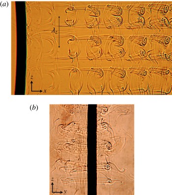
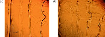
For large Froude numbers, the 2D wake is destabilized when the Reynolds number increases above 190. Figure 3 shows the periodic structures with a well-defined wavelength which are created approximately 5 diameters downstream of the cylinder. These structures are characteristic of the classical mode A, well-known in a homogeneous fluid. Indeed, the side view is very similar to the dye visualization of figure 13 in Williamson (Reference Williamson1996a ), with longitudinal vortices whose tails are stretched toward the cylinder. The front view of figure 3(b) clearly shows that these vortices are counter-rotating vortex pairs perpendicular to the von Kármán vortices.
Shadowgraph visualizations of the mode A: the wake behind a vertical cylinder is obtained at Reynolds number
 $\mathit{Re}=190$
and Froude number
 $F=4$
. In the side view (a), the cylinder is moving to the left. In the front view (b) the cylinder is moving toward the observer with a very small angle in order to see the structures on the right-hand side of the cylinder. The field of view is approximately
 $8\times 15$
diameters in the side view.

Moreover, the wavelength of this mode is close to 4 diameters, which is in excellent agreement with the theoretical value
 ${\it\lambda}_{z}/D=3.96\pm 0.02$
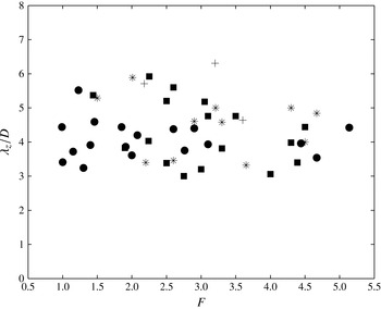
obtained by Barkley (Reference Barkley1996) for the mode A. The wavelength of this mode has been measured for different Froude numbers. It is calculated as the average over 4 wavelengths in
 $Z$
and over 4–5 different images. This leads to an uncertainty of the order of 20 %. It is plotted in figure 4 and seems to be independent of the Froude number within the noise in the measurement (of the order of 20 %).
Plot of the wavelength
 ${\it\lambda}_{z}$
of the mode A non-dimensionalized by
 $D$
for different values of Froude number at a Reynolds number between 180 and 190, for different tilt angles
 ${\it\alpha}$
in the experiments: circles are for the vertical cylinder, squares for
 ${\it\alpha}=30^{\circ }$
, crosses for
 ${\it\alpha}=45^{\circ }$
and stars for
 ${\it\alpha}=60^{\circ }$
.

This mode A is the first 3D unstable mode when the cylinder is tilted with an angle smaller than 45°. For all tilt angles, the spatial structure is the same of the vertical cylinder. The wavelength remains unchanged as can be seen on figure 4. However, the critical Reynolds number strongly varies with the Froude number and the tilt angle as will be shown in the next section.
3.2. Stability diagram
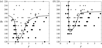
By varying the velocity and the diameter of the cylinders, it is possible to vary independently the Reynolds number and the Froude number. We have done different experiments in order to determine the stability of the 2D flow as a function of the Reynolds number and the Froude number. These results are reported in figure 5(a), where circles correspond to a 2D flow and stars correspond to mode A. This stability diagram allows the determination of the critical Reynolds number
 $\mathit{Re}_{c}$
at which the flow becomes 3D as a function of the Froude number (plotted as a solid line). At large Froude number, the critical Reynolds number tends to
 $\mathit{Re}_{c}=185\pm 5$
. This result is satisfying because for these weak stratifications, the dynamics of the wake is expected to be the same than for a homogeneous cylinder wake, where the critical Reynolds number is equal to 189 (Barkley Reference Barkley1996).
Stability diagrams of the 3D instabilities in the stratified wake of (a) a vertical cylinder and (b) a cylinder tilted at an angle
 ${\it\alpha}=30^{\circ }$
in the cross-stream section. Black circles correspond to stable experiments and stars correspond to the mode A. The open star in (a) corresponds to the experiment shown in figure 3. The solid lines correspond to the limit of stability found experimentally; grey diamonds correspond to the critical Reynolds number obtained numerically.

For moderate Froude numbers (
 $1\leqslant F\leqslant 4$
), the critical Reynolds number decreases with a minimum of
 $\mathit{Re}_{c}=130$
at
 $F=1.5$
. This indicates that a moderate stratification seems to increase the destabilization of the 3D mode A (which is at the origin of the mode A). It is surprising to observe that stratification can destabilize the flow because stratification is known to stabilize the elliptical instability, as it tends to prevent the appearance of von Kármán vortices due to the stabilization of shear flows. This is claimed to be at the origin of mode A (Williamson Reference Williamson1996b
; Leweke & Williamson Reference Leweke and Williamson1998; Thompson et al.
Reference Thompson, Leweke and Williamson2001). Indeed, Kerswell (Reference Kerswell2002) showed using a local approach that the growth rate
 ${\it\sigma}$
of the elliptical instability is given by
 $$\begin{eqnarray}\displaystyle {\it\sigma}=\frac{9}{16}{\it\epsilon}\left(1-\frac{3}{4F_{v}^{2}}\right), & & \displaystyle\end{eqnarray}$$
in the presence of a weak stratification (the case of inviscid fluid). Here, the vortex Froude number
 $F_{v}={\it\Omega}_{0}/N$
is based on the angular velocity
 ${\it\Omega}_{0}$
at the core of the vortex and
 ${\it\epsilon}$
corresponds to the ellipticity of the streamlines. This equation indicates that the growth rate decreases in the presence of an increasing but still weak stratification, which would correspond to a stabilization of the mode A. This is opposite to the experimental observations where a weak and moderate stratification increases the destabilization of the mode A.
To understand this difference, we have calculated analytically the growth rate of the elliptical instability for a Gaussian vortex in a stratified fluid, using a global approach instead of the local approach used by Kerswell (Reference Kerswell2002). The calculation, detailed in the appendix A, is very similar to the calculation done in Guimbard et al. (Reference Guimbard, Le Dizès, Le Bars, Le Gal and Leblanc2010) for the elliptic flow in a rotating stratified cylinder. Unfortunately, the analytical growth rate is very close to the local theory and leads to the same conclusion, i.e. a stabilization for weak stratification. A possible explanation for this discrepancy may be due to the fact that the elliptical instability is calculated for a single vortex whereas the mode A is a global mode for the whole von Kármán vortex street. It is indeed possible that the group velocity of the 3D perturbation increases with the stratification such that the instability becomes absolutely unstable for smaller Reynolds numbers than without stratification.
However, when the Froude number is decreased below 1.5 the stratification has a drastic stabilization effect. Indeed the critical Reynolds number strongly increases by 50 % between
 $F=1.5$
and
 $F=0.5$
. This is probably due to the appearance of critical layers in the Kelvin modes of a stratified Gaussian vortex, which creates a strong dissipation (Le Dizès Reference Le Dizès2008).
When the cylinder is slightly tilted in the cross-stream section (
 $0^{\circ }\leqslant {\it\alpha}\leqslant 30^{\circ }$
), the mode A is still observed. The stability diagram has also been established for
 ${\it\alpha}=30^{\circ }$
(see figure 5
b). The variation of the critical Reynolds number with the Froude number is similar to the case of the vertical cylinder. Mode A is destabilized for
 $1.5<F<4$
and stabilized for
 $F<1.5$
. However, the destabilization is weaker for the tilted cylinder (with a minimum
 $\mathit{Re}_{c}=150$
) than for the vertical case (with a minimum
 $\mathit{Re}_{c}=130$
). This indicates that the tilt of the cylinder tends to stabilize the mode A. This is even clearer at larger angle as will be shown in § 4.
3.3. Numerical simulation
The critical Reynolds number has also been calculated numerically using the Navier–Stokes equations linearized around the 2D base flow. The perturbation is assumed to be sinusoidal in
 $z$
, with a fixed wavenumber
 $k$
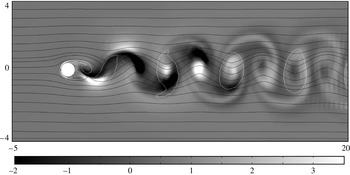
, as given by (2.3). This method is similar to the Floquet analysis done by Barkley (Reference Barkley1996). Figure 6 is an example of the numerical result obtained by Comsol. In this figure, the white contours of vorticity indicate the position of the 2D von Kármán vortices and the greyscale corresponds to the axial velocity of the 3D perturbation
 $w_{1}$
. In each vortex, there are two lobes of axial velocity, one positive and one negative. This is especially visible in the second and third vortices. It corresponds to the spatial structure of the elliptic instability, as noted by Thompson et al. (Reference Thompson, Leweke and Williamson2001) for mode A.
Axial velocity of the 3D perturbation
 $w_{1}$
obtained numerically for a vertical cylinder in the (
 $x,y$
) plane at
 $\mathit{Re}=190$
and
 $F=4$
. Solid lines are the streamlines of the 2D flow
 $(u,v)$
corresponding to a von Kármán street. White contour lines correspond to the vorticity. The field of view is
 $16\times 8$
diameters.

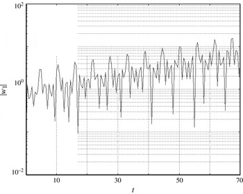
In order to determine the growth of the perturbation, the axial velocity
 $w_{1}$
is measured at
 $x=5$
and
 $y=0.5$
, i.e. at the position where the maximum of axial velocity passes periodically. It is plotted in figure 7 as a function of time and indeed exhibits periodic peaks of velocity. Moreover, the amplitude of these peaks increases exponentially with time and grows by almost one decade between
 $t=0$
and
 $t=70$
. Fitting the maxima with an exponential function
 $\exp ({\it\sigma}t)$
allows the growth rate
 ${\it\sigma}$
to be determined for a given Reynolds number, Froude number and wavenumber.
Temporal variation of the absolute value
 $|w_{1}|$
of the axial velocity of the perturbation. The velocity is evaluated at
 $(x,y)=(5,0.5)$
.
 $\mathit{Re}=220$
,
 $F=3$
.

To determine the critical Reynolds number, the maximal wavenumber
 $k_{max}$
corresponding to the most unstable mode is sought for each Froude number and Reynolds number. To do so, the instability growth rate
 ${\it\sigma}$
is measured for three values of
 $k$
around the maximum and fitted by a parabola. In fact, it was found that
 $k_{max}\simeq 1.5$
is almost independent of the Froude and the Reynolds number, in agreement with the experimental results. Then, the maximum growth rate
 ${\it\sigma}$
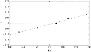
is calculated for different values of Reynolds number. As shown on figure 8, it increases linearly with the Reynolds number. The critical Reynolds number
 $\mathit{Re}_{c}$
simply corresponds to the Reynolds number at which the growth rate
 ${\it\sigma}$
vanishes.
Growth rate of the instability for different Reynolds numbers at
 $F=4$
with
 $k=k_{max}=1.5$
. Black symbols correspond to numerical data and the dashed line is a linear fit of the numerical points.

This critical Reynolds number is calculated for various Froude numbers
 $F$
. It is plotted in figure 5 as grey diamonds. It is very close to the experimental critical Reynolds number (plotted as a solid line), although it seems to be slightly above the experimental value. This is probably due to the subcriticality of this transition which imposes that the linear threshold is above the nonlinear threshold. However, the most important result is that the critical Reynolds number indeed decreases down to 130 when the Froude number is equal to 1.5. This is a good confirmation of the destabilization of the mode A by a weak to moderate stratification.
4. Mode S: the instability of tilted cylinders
4.1. A new unstable mode
The previous section showed that the mode A is the first unstable mode for weakly tilted cylinders. This dynamics is strongly modified when the tilt angle
 ${\it\alpha}$
is increased above 45°. Indeed, a new unstable mode appears in a region of moderate stratification
 $(1.5\leqslant F\leqslant 3.5)$
. Figure 9 shows side shadowgraph views of this unstable mode, which is characterized by axial lines undulating at a well-defined wavelength. It should be mentioned that for this tilt angle, the lines are present below the critical Reynolds number (
 $\mathit{Re}\leqslant 140$
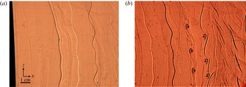
), but they remain straight. This indicates that these lines are created by the two-dimensional base flow. In the shadowgraph visualizations, they reveal layers of strong density gradients. It can be noted that they appear alternately dark and white probably because the von Kármán vortices are alternate. Above the critical Reynolds number, these straight lines begin to undulate. The undulations grow with time describing S-shaped structures far from the cylinder. This is why this mode has been called mode S. The dimensionless wavelength of this structure is
 ${\it\lambda}_{z}/D\simeq 4$
which is the same as for the mode A discussed previously.
Shadowgraph side view visualizations of the mode S: the wake behind a cylinder is tilted at
 ${\it\alpha}=45^{\circ }$
for
 $\mathit{Re}=170$
and
 $F=2.5$
. The cylinder is moving to the left and there is a time delay of approximatively
 $6D/U$
between (a) and (b) to reveal the temporal evolution of the instability. The field of view is approximately
 $8\times 15$
diameters.

The undulations seem to reveal lines of co-rotating vortices, as drawn schematically with arrows in figure 9(b). This could correspond to Kelvin–Helmholtz billows of a vertical shear layer. It should be noted that the shear is opposite for the white and the dark layers, since the vortices have opposite rotating directions.
4.2. A tilt-induced instability
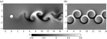
In order to understand the structure and the origin of this instability, the 2D dynamics has been analysed numerically using Comsol. Figure 10(a) shows that the 2D base flow is characterized by strong axial velocities which can be as large as the incoming flow. The axial velocity is confined in mushroom-like structures between the von Kármán vortices. The velocity is alternately positive and negative, which can explain the fact that the lines are alternately white and black in the shadowgraph visualizations of figure 9. These mushroom-like structures are actually due to the tilted vortices. Indeed, we show in the following that they can be explained by the critical layers appearing in each tilted vortex.
Axial velocity
 $w_{2\mathit{D}}$
of the 2D base flow obtained (a) by a 2D numerical simulation in the
 $(x,y)$
plane and (b) for the axial flow generated by two lines of alternate vortices (expression for a single vortex given by (4.1). The tilt angle
 ${\it\alpha}=45^{\circ }$
, the Reynolds number
 $\mathit{Re}=180$
and the Froude number
 $F=2.5$
are chosen where the mode S is observed experimentally. Black and white contours correspond to negative and positive vorticity.

Boulanger et al. (Reference Boulanger, Meunier and Le Dizès2006) have shown that the inviscid solution of a solitary vortex (tilted with respect to the stratification) exhibits a divergence of the axial velocity at the critical radius
 $r_{c}$
where the angular velocity of the vortex
 ${\it\Omega}(r_{c})$
is equal to the Brunt–Väisälä frequency. Using a viscous critical layer analysis, they found that close to
 $r_{c}$
, the velocity has the form:
 $$\begin{eqnarray}\displaystyle w_{2\mathit{D}}(r)=\frac{{\rm\pi}r_{c}{\it\Omega}^{2}(r_{c})}{|2{\it\Omega}^{\prime 2}(r_{c})|^{2/3}}H_{i}[\text{i}|2{\it\Omega}^{\prime 2}(r_{c})|^{1/3}(r-r_{c})\mathit{Re}^{1/3}], & & \displaystyle\end{eqnarray}$$
where
 ${\it\Omega}^{\prime }(r_{c})$
represents the derivative of the angular velocity and
 $H_{i}$
corresponds to the Scorer function. This theoretical solution is plotted for each von Kármán vortex in figure 10(b). To do so, the positions of the vortices are extracted from figure 10(a) and the profile of angular velocity is chosen as
 ${\it\Omega}(r)={\it\Gamma}[1-\exp (-r^{2}/a^{2})]/(2{\rm\pi}r^{2})$
with
 $a=0.7D$
and
 ${\it\Gamma}=\pm 2.31UD$
in order to represent the von Kármán vortices of figure 10(a). It is clear that the interference of the critical layers generates mushrooms of axial velocity with alternately positive and negative sign, as in the numerical simulation. The amplitude of the axial velocity is of the same order in the theory and in the numerics. But the thickness of the structures seems to be larger in the numerics than in the theory. This is probably due to numerical diffusion inherent in the finite-element method used by Comsol.
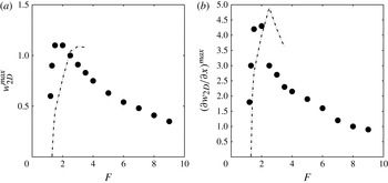
A quantitative comparison of this model with the numerics can be done by plotting the maximum axial velocity
 $w_{2D}^{max}$
of the 2D base flow for different Froude numbers (figure 11
a). It can be noted that
 $w_{2D}^{max}$
increases drastically at
 $F\simeq 1$
. This transition corresponds to the appearance of the critical layer (which does not exist for small
 $F$
because
 ${\it\Omega}(r)<N$
for all
 $r$
). The maximum value of the axial velocity
 $w_{2D}^{max}$
is reached at
 $F\simeq 2$
and is slightly larger than 1. For larger Froude numbers, the axial velocity
 $w_{2D}^{max}$
decreases gradually. The theoretical prediction of
 $w_{2D}^{max}$
is plotted as a dashed-dotted line in figure 11(a). It is in good quantitative agreement with the numerics at small Froude numbers. However, this theory can only be used for moderate Froude numbers because at large Froude numbers the vortices cannot be considered as solitary, the critical layers being larger than the distance between vortices.
Maximum value of (a) the axial velocity
 $w_{2D}$
and (b) the shear
 $\partial w_{2D}/\partial x$
as a function of the Froude number. Black symbols represent the numerical data and dashed lines represent the theoretical prediction.
 $\mathit{Re}=180$
,
 ${\it\alpha}=45^{\circ }$
.

Figure 11(b) shows the maximum of the axial shear
 $\partial w_{2D}/\partial x$
. The shear suddenly increases at
 $F\simeq 1$
and reaches a maximum of the order of 5 at
 $F\simeq 2$
. For larger
 $F$
the shear gradually decreases. There is again a good agreement between the theory and the numerics.
These results clearly prove that the strong axial velocity and strong shear present in the base flow are due to the critical layers of the von Kármán vortices. Moreover, these high shears are largest for moderate Froude numbers (
 $1.5<F<4$
), i.e. exactly where the mode S is observed in the experiments. This indicates that the mode S is simply a Kelvin–Helmholtz instability of these strong shears, as was observed for solitary tilted vortices by Boulanger et al. (Reference Boulanger, Meunier and Le Dizès2007). Indeed, the shear
 $\partial w_{2D}/\partial x$
generates cross-stream Kelvin–Helmholtz billows on an axial line, as observed on figure 9(b).
4.3. Stability diagram
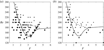
The experimental and numerical results concerning the 3D stability of the cylinder wake are presented for
 ${\it\alpha}=45^{\circ }$
(figure 12
a) and
 ${\it\alpha}=60^{\circ }$
(figure 12
b). The same trend is observed for these two angles. At large Froude number, the critical Reynolds number for the mode A tends to 190 as it is the case for a homogeneous fluid. For moderate stratification (
 $2\leqslant F\leqslant 4$
), there is a range of Reynolds number (
 $140<\mathit{Re}<190$
), where the mode A is stable whereas the mode S is unstable. However, the mode A is always observed at large Reynolds number. This indicates that the mode A is always dominant with respect to the mode S when it is unstable.
Stability diagrams of a cylinder wake tilted (a) at
 ${\it\alpha}=45^{\circ }$
and (b) at
 ${\it\alpha}=60^{\circ }$
for different Reynolds and Froude numbers. Circles correspond to stable experiments, stars to the mode A and squares to the mode S. The open star in (a) corresponds to the experiment shown in figure 9. The transition between a stable and unstable domain is represented by the black lines and the mode S/mode A transition is represented by a grey dashed lines. The grey diamonds in (a) correspond to the critical Reynolds number obtained numerically.

For small Froude number (
 $F\leqslant 1.5$
), the critical Reynolds number strongly increases for strong stratification. The von Kármán street can be observed without a 3D structure up to
 $\mathit{Re}=250$
. It highlights the fact that the wake is strongly stabilized by a strong stratification. However, the small dimensions of the tank used in the experiments do not allow study of very small Froude numbers; it would require large cylinder diameters, which would reduce the aspect ratio below 10, leading to strong end effects. It is thus unclear what other instabilities would appear for very small Froude numbers (
 $F<0.1$
) where a zigzag instability might be observed (Deloncle, Billant & Chomaz Reference Deloncle, Billant and Chomaz2011). We have tried to visualize the zigzag instability using larger cylinder diameters but it has not been observed with this experiment probably due to the small dimensions on the tank for that range of diameters (
 $D>32\ \text{mm}$
).
The critical Reynolds number has been calculated numerically at
 ${\it\alpha}=45^{\circ }$
. It seems to be close to the value where the mode A appears in the experiments. This indicates that the mode S has not been observed numerically. This is probably due to the weak spatial resolution used when the 3D perturbation is calculated. This introduces a strong numerical diffusion which tends to attenuate the critical layers and thus damp the mode S. Moreover, these numerical simulations become very noisy when the tilt angle increases. They have not been done for tilt angles larger than 45°.
5. Rayleigh–Taylor mode
In this section, the case of very large tilt angle (
 ${\it\alpha}\in [60^{\circ },85^{\circ }]$
) and large Froude number (i.e. weak stratification) is studied.
5.1. Shadowgraph study
For nearly horizontal cylinders, a new instability appears at weak stratification. Top shadowgraph views are presented figure 13 for a Reynolds number
 $\mathit{Re}\simeq 180$
and a Froude number
 $F\simeq 8.5$
. Under the threshold, straight layers can be seen as in the case of the mode S. Above the threshold these layers are deformed by counter-rotating vortices, creating rolls oriented along the
 $(Ox)$
axis, similar to the plumes appearing in Rayleigh–Taylor instabilities. This is why this mode has been called mode RT.
Top shadowgraph visualizations of the mode RT: the wake behind a cylinder tilted at
 ${\it\alpha}=75^{\circ }$
with respect to the vertical, obtained at
 $\mathit{Re}=175$
and
 $F=8.5$
. The picture (b) is obtained a time delay
 $3D/U$
after (a) which is obtained
 $6D/U$
downstream of the cylinder. The cylinder is moving to the left. The field of view is approximately
 $8\times 15$
diameters.

This mode is characterized by counter-rotating vortices behind the cylinder as was observed for the mode A. But this new instability presents some differences. First, the tails of the vortices seem to be stretched in the opposite direction (i.e. downstream for this mode and upstream for the mode A). Then, these counter-rotating vortices are very far from the cylinder: they appear approximately 15 diameters downstream of the cylinder whereas the mode A appeared 4 diameters downstream. Finally, the dimensionless wavelength
 ${\it\lambda}_{z}/D\simeq 3$
is smaller than the wavelength of the mode A (
 ${\it\lambda}_{z}/D\simeq 4$
), although it is not very periodic.
5.2. Structure of the base flow
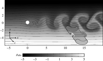
A 2D numerical study has been used to check if the base flow may be unstable with respect to the Rayleigh–Taylor instability. The absolute density of the 2D base flow
 ${\it\rho}_{abs}={\it\rho}_{2\mathit{D}}+\bar{{\it\rho}}={\it\rho}_{2\mathit{D}}+y\sin {\it\alpha}$
has been plotted in a nearly vertical plane (see figure 14). In this figure, heavy (respectively light) mushrooms appear, due to the advection of heavy (resp. light) fluid by the von Kármán vortices. These structures highlight the fact that heavier fluid can be located above lighter fluid. This overturning of the mean density is unstable with respect to the Rayleigh–Taylor (gravitational) instability. Since these heavy/light mushrooms are invariant along the
 $z$
direction (see 3D drawing in figure 14), they can be subject to an instability with a large axial wavelength. This leads to convective rolls perpendicular to the
 $(Oz)$
direction, i.e. oriented along the
 $(Ox)$
axis (see 3D sketch in figure 14). This is exactly what has been observed in the shadowgraph visualization of figure 13.
Absolute density
 ${\it\rho}_{abs}={\it\rho}_{2\mathit{D}}+\bar{{\it\rho}}$
of the base flow obtained numerically for a cylinder in the
 $(x,y)$
plane with a tilt angle
 ${\it\alpha}=75^{\circ }$
and for
 $\mathit{Re}=170$
and
 $F=8$
. Solid lines correspond to the streamlines of the 2D flow (
 $u,v$
) corresponding to a von Kármán street. The field of view is
 $16\times 6$
diameters.

The mode RT appears far from the cylinder because it is due to the overturning. The density diffuses much slower than the vorticity such that the base flow remains unstable over large downstream distances. By contrast, the mode A is localized very close to the cylinder because it is driven by the velocity of the vortices which decreases rapidly at these Reynolds numbers.
5.3. Stability diagram
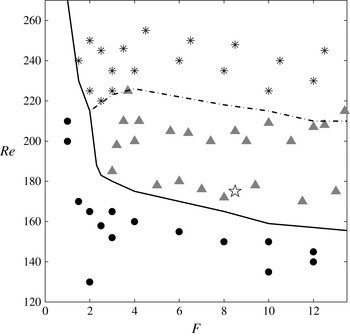
The experimental results concerning the 3D stability of the cylinder wake for
 ${\it\alpha}=75^{\circ }$
are presented in figure 15. The mode RT appears for very weak stratifications since it has been visualized for Froude numbers as large as 15. The critical Reynolds number is of the order of 180 for moderate Froude numbers (
 $F\simeq 3$
) and decreases down to 150 for large Froude numbers. It thus seems that when the stratification becomes weaker the mode RT becomes more unstable. This is surprising because the mode RT is linked to the density differences of the mushroom structures which should increase with the background density gradient. However, it is possible that at moderate Froude numbers, the background stratification prevents overturning which suppresses the Rayleigh–Taylor instability. This corresponds with the complete suppression of von Kármán vortices by the stratification, which occurs for example at
 $F=1.7$
for
 $\mathit{Re}=150$
(Meunier Reference Meunier2012a
).
Stability diagram for a cylinder wake tilted at
 ${\it\alpha}=75^{\circ }$
. Circles correspond to stable experiments, grey triangles to experiments where the mode RT is observed and stars to mode A. The open star corresponds to the experiment shown in figure 13. The stable and unstable domains are separated by a black dashed line and the mode RT and the mode A are separated by a dash-dotted line.

At this tilt angle, the mode A can still be visualized but it is not the first unstable 3D mode. It appears for a critical Reynolds number varying from
 $\mathit{Re}\simeq 220$
to
 $\mathit{Re}\simeq 190$
when the Froude number increases from 2 to 12, which is slightly above the critical Reynolds number of the mode RT. However, the mode A seems to be dominant compared to the mode RT (when it is unstable), probably because the mode A is located very close to the cylinder.
6. Mode L
In this section, the cylinder is still tilted with an angle close to
 ${\it\alpha}=75^{\circ }$
but the fluid is now strongly stratified (
 $0.1\leqslant F\leqslant 1$
).
6.1. Experimental visualizations
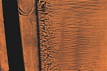
Figure 16 presents the shadowgraph view of the instability appearing for a Reynolds number
 $\mathit{Re}=110$
and a Froude number
 $F=0.55$
. In this image, a uniform zone is observed just behind the cylinder which extends over 1 diameter. A dark axial line separates this zone from a highly disturbed region, with small-scale structures which give rise further downstream to thin streamwise lines. The wavelength of this instability is dramatically smaller compared to the previous modes since it is of the order of 0.3 diameters (which is 10 times smaller than the wavelength of mode A or mode S). It should be mentioned that the cylinder seems to be tilted in this image, but this is simply due to a deformation by the lens of the shadowgraph.
Top shadowgraph visualization of the mode L for
 $\mathit{Re}=110$
,
 $F=0.55$
and
 ${\it\alpha}=75^{\circ }$
. The cylinder is moving to the left. The field of view is approximately
 $8\times 15$
diameters.

An important aspect of this unstable mode is that it can appear in the absence of von Kármán vortices in the base flow. This is totally different from the three other modes which rely on the presence of von Kármán vortices. A dye visualization of the 2D base flow has been done at the same parameters where this mode is observed (
 $\mathit{Re}=110$
,
 $F=0.55$
). As can be seen on the side view of figure 17, the 2D base flow does not contain a von Kármán vortex street. In this image, the recirculation bubble present behind the cylinder is very short. But there is a second recirculation bubble approximately 1.5 diameters downstream of the cylinder. This is in agreement with the visualizations of Boyer et al. (Reference Boyer, Davies, Fernando and Zhang1989) who called these bubbles isolated mixed regions. We also observe a small third recirculation bubble further downstream.
Dye visualization from the side of the tank for the same Reynolds number
 $\mathit{Re}=110$
, Froude number
 $F=0.55$
and angle
 ${\it\alpha}=75^{\circ }$
as in figure 16. The cylinder is moving to the left. The field of view is approximately
 $3\times 15$
diameters in the side view, i.e. in the
 $(X,Z)$
plane.

Such an isolated recirculation bubble has also been observed by Baines & Hoinka (Reference Baines and Hoinka1985) behind a semi-circular hill in a narrow range of Froude numbers. The size of the recirculation bubble has been shown to scale as
 $U/N$
by Sutherland (Reference Sutherland2002).
Comparing figures 16 and 17 indicates that the thick dark axial line of the shadowgraph visualizations is located very close to the upstream end of the second recirculation bubble. It means that the 3D instability is generated near the upstream stagnation point of the recirculation bubble. This is not surprising since the streamwise velocity vanishes at this point, such that any convective instability may become absolutely unstable close to this point.
6.2. A numerical clue
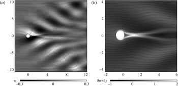
In order to understand the origin of this mode, some 2D numerical simulations have been carried out to characterize the base flow. Figure 18 represents the axial velocity
 $w_{2D}$
obtained numerically for
 $\mathit{Re}=110$
,
 $F=0.65$
and
 ${\it\alpha}=75^{\circ }$
, i.e. where the mode L has been visualized. The streamlines undulate downstream of the cylinder because of the lee waves, which propagate at an angle of approximately 30° with respect to the
 $x$
axis. However, since the cylinder is tilted, these lee waves contain some axial velocity (Meunier Reference Meunier2012b
), which is visible as an alternation of white and black lobes along two oblique directions.
Numerical simulations for a tilt angle
 ${\it\alpha}=75^{\circ }$
in the
 $(x,y)$
plane at
 $\mathit{Re}=110$
and
 $F=0.65$
. The greyscale represents in (a) the axial velocity
 $w_{2D}$
and in (b) the derivative of the axial velocity
 $\partial w_{2D}/\partial y$
. Dark lines correspond to the streamlines.

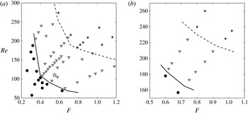
Stability diagrams for strong stratifications and large tilt angles: (a)
 ${\it\alpha}=75^{\circ }$
and (b)
 ${\it\alpha}=82.5^{\circ }$
. Circles correspond to stable experiments, grey triangles to experiments with the mode L and stars to experiments with the mode A. The open star in (a) corresponds to the experiment shown in figures 16 and 17.

These axial velocities obviously create a strong shear
 $\partial w_{2\mathit{D}}/\partial y$
as indicated in figure 18(b). The shear is particularly large on the centreline between the first and second recirculation bubbles, where it is of the order of
 $2U/D$
. This shear may thus be unstable with respect to the Kelvin–Helmholtz instability. This would indeed generate Kelvin–Helmholtz billows oriented along the
 $x$
axis, which could correspond to the thin streamwise lines visible in figure 16. However, estimating the thickness of the shear layer as
 ${\it\delta}\simeq D/2$
allows an estimate of the wavelength of
 ${\it\lambda}_{z}\simeq 3D$
to be deduced, corresponding to the most unstable wavelength of the Kelvin–Helmholtz instability. This wavelength is 10 times larger than the wavelength observed in the experiment (
 ${\it\lambda}_{z}\simeq 0.3D$
). This difference may probably be due to the hyperbolic point located at the second recirculation bubble which may greatly modify the characteristics of the Kelvin–Helmholtz instability.
6.3. Stability diagram
Stability diagrams for
 ${\it\alpha}=75^{\circ }$
(figure 19
a) and for
 ${\it\alpha}=82.5^{\circ }$
(figure 19
b) have been constructed at very small Froude numbers (
 $F\leqslant 1$
). The mode L is represented by grey triangles. It has been observed for relatively small Reynolds numbers compared to the other unstable modes. Indeed, it can be observed for Reynolds numbers as low as 60 for
 ${\it\alpha}=75^{\circ }$
.
Regarding the other modes, the mode A is observed at larger Reynolds numbers (represented as stars on the diagrams). It should be noted that the mode L does not appear for very small Froude numbers (
 $F<0.4$
at
 ${\it\alpha}=75^{\circ }$
). This is surprising because lee waves are expected to be present at very small Froude numbers, as is supposed for strongly stratified fluids, but in our experiments no lee wave mode was observed for
 $F<0.4$
.
Radial profile of the strain
 $f(r)$
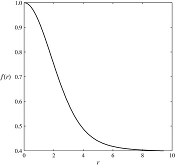
in a vortex with a Gaussian vorticity deformed elliptically by the flow (A 4).

This mode has not been observed for a horizontal cylinder. This is probably due to the lack of axial velocity in the lee waves at
 ${\it\alpha}=90^{\circ }$
(due to the symmetry of the problem). This mode is already more stable at
 ${\it\alpha}=82.5^{\circ }$
than at
 ${\it\alpha}=75^{\circ }$
, as can be inferred by comparing figures 19(a) and 19(b). For example, for a Froude number
 $F=0.7$
, the critical Reynods number
 $\mathit{Re}_{c}$
is smaller at
 ${\it\alpha}=75^{\circ }$
than at
 ${\it\alpha}=82.5^{\circ }$
(comparing figures 19(a) and 19(b), it can be seen that
 $\mathit{Re}_{c}=70$
at
 ${\it\alpha}=75^{\circ }$
whereas
 $\mathit{Re}_{c}=165$
at
 ${\it\alpha}=82.5^{\circ }$
). This mode is thus limited to nearly horizontal but tilted cylinders (
 $65^{\circ }<{\it\alpha}<85^{\circ }$
).
7. Conclusion
In this paper, an experimental study has been carried out of a stratified wake of a circular cylinder in order to describe the effect of the tilt and of the stratification on the 3D instabilities of the wake.
Primarily, it was shown that the classical mode A, well-known in homogeneous cylinder wakes, remains present for weak stratifications (i.e. for large Froude numbers). This mode is made of counter-rotating vortex pairs which appear close to the cylinder. The dimensionless wavelength of this mode is close to 4 as for homogeneous fluids and is independent of the Froude number. Although for weak stratification the critical Reynolds number is close to 190 (as for homogeneous fluids), this mode appears at a smaller Reynolds number for moderate stratifications if the cylinder is nearly vertical. This destabilization seems to be in contradiction with the stabilization of the elliptical instability (which is at the origin of mode A) by the stratification predicted theoretically by Kerswell (Reference Kerswell2002). However, the mode A is stabilized by a strong stratification. A numerical study has been done, showing a good agreement between the experimental and numerical critical Reynolds numbers.
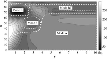
Figure 21 presents the critical Reynolds number at which the wake becomes three-dimensional for all Froude numbers
 $F$
and tilt angles
 ${\it\alpha}$
. The mode A is the first unstable mode for a large range of Froude numbers (
 $0.1\leqslant F\leqslant 10$
) but only for small tilt angles (
 $0^{\circ }\leqslant {\it\alpha}\leqslant 60^{\circ }$
).
Critical Reynolds number
 $\mathit{Re}_{c}$
of the appearance of a 3D unstable mode as a function of the tilt angle
 ${\it\alpha}$
and the Froude number
 $F$
. White contours indicate the first unstable mode.

For moderate tilt angles a new unstable mode, called mode S, appears at moderate stratification. This mode, characterized by dark and bright undulated layers, reveals the presence of co-rotating vortices. A 2D numerical study, coupled to the theoretical structure of critical layers inside each von Kármán vortex, has shown that these co-rotating vortices are simply Kelvin–Helmholtz billows of the strong shears generated by the axial velocity of the 2D flow. This is similar to the tilt-induced instability of a solitary vortex tilted with respect to the stratification (Boulanger et al.
Reference Boulanger, Meunier and Le Dizès2007). As shown in figure 21, the mode S appears in a very narrow region of parameters, i.e. for moderate stratification (
 $1.5\leqslant F\leqslant 3.5$
) and moderate tilt angles (
 $40^{\circ }\leqslant {\it\alpha}\leqslant 70^{\circ }$
).
For large tilt angles (
 $65^{\circ }<{\it\alpha}<85^{\circ }$
), two other unstable modes have been discovered (see figure 21). For a weak stratification (
 $3<F<10$
), shadowgraph visualizations reveal the presence of counter-rotating vortices far from the cylinder. These vortices seem to be convective rolls created by a Rayleigh–Taylor (gravitational) instability. This explanation is confirmed numerically by the presence of overturning generated by the 2D base flow. This mode has thus been called mode RT.
For large tilt angles and for strong stratifications, the dynamics is strongly modified since three-dimensional instabilities appear even in the absence of von Kármán vortices, i.e. for a stationary flow. This mode is due to the presence of lee waves emitted by the cylinder, which contain some axial velocity if the cylinder is tilted. It leads to a strong shear on the centreline downstream of the cylinder which creates streamwise Kelvin–Helmholtz billows. This mode, which has been called mode L (for lee-wave mode), is characterized by a very small axial wavelength of the order of 0.3 diameter. This mode is observed for small Froude numbers (
 $0.4<F<2$
) and nearly horizontal but tilted cylinders, as shown on figure 21.
These results highlight the fact that the stratification strongly modifies the transition from a 2D to a 3D flow in a cylinder wake, with the presence of three new unstable modes. The tilt of the cylinder with respect to the vertical plays a major role, such that a study limited to a vertical or a horizontal cylinder misses a lot of the rich dynamics of the tilted wake.
This is particularly interesting for geophysical applications where stratified wakes have been usually restricted to 2D horizontal bluff bodies. For example, in oceans, the wake of a coastal tip may be influenced by the weak inclination of the continental slope such that the wake may become unstable with respect to the mode L instead of being unstable with respect to the mode A as for a horizontal object. The structure of the unstable mode leads to different characteristics (wavelength, orientation of the structures) which may lead to very different mixing and turbulent stresses.
However, because this study is limited to a fundamental bluff body like the cylinder, it is very far from real geophysical applications. It would be interesting to see whether the rich dynamics described in this paper is still present in the wake of a ridge or a half-cylinder on a tilted plane. The presence of the boundary will modify the structure of the von Kármán wake, which may suppress some unstable modes but also create some new unstable modes. Moreover, the presence of the boundary layer on the tilted plane may also modify the whole dynamics of the stratified wake.
In fact, stratified boundary layers over a tilted bottom have received little attention and deserve more work. Candelier, Le Dizès & Millet (Reference Candelier, Le Dizès and Millet2012) have shown theoretically that they are subject to a radiative instability which may be more unstable than the destabilization of Tolmien-Schlichting waves. Moreover, Passaggia, Meunier & Le Dizès (Reference Passaggia, Meunier and Le Dizès2014) have recently shown numerically that an undulation of the topography generates a critical layer inside the boundary layer, with strong cross-stream flows. It is clear that experiments are needed to confirm and characterize these complex phenomena. To this end, a new tank is being built in our laboratory, which will allow the study of the boundary layer of a tilted plane in a background stratification.
Finally, there have been very few numerical studies on the stratified wake of a tilted cylinder. The 2D dynamics has been characterized by Meunier (Reference Meunier2012a ) but the 3D dynamics has never been studied in detail. High-level Floquet analysis and DNS would probably give more information on the structure and the mechanism of the unstable modes.
Acknowledgements
The authors would like to thank Dr J. Leontini who helped writing the numerical procedure for the 3D linear stability analysis. This study has been done under the grant ANR 11 BS56 012 01 from the French government.
Appendix A. Calculus of the global growth rate of the elliptic instability for a Gaussian stratified vortex
In this appendix, the details of the calculus evoked in § 3 concerning the mode A are developed. This calculus has the purpose of verifying the local theory given by Kerswell (Reference Kerswell2002) for the growth rate of the elliptic instability in a stratified fluid. An inviscid study is done here using a global approach analysing the coupling of Kelvin modes via the ellipticity.
A.1. Definition of the velocity and calculus of the elliptical base flow
The question is to know if a 2D stratified and vertical vortex with elliptic streamlines can be unstable with respect to a 3D perturbation
 $\boldsymbol{u}^{\prime }$
which grows in time with a growth rate
 ${\it\sigma}$
. The total velocity is thus decomposed into three terms:
 $$\begin{eqnarray}\boldsymbol{u}_{tot}=\boldsymbol{u}+{\it\epsilon}\boldsymbol{u}_{ell}+\boldsymbol{u}^{\prime }\end{eqnarray}$$
where the 2D base flow is the sum of an axisymmetric vortex
 $\boldsymbol{u}$
and a small ellipticity
 ${\it\epsilon}\boldsymbol{u}_{ell}$
. The axisymmetric vortex is characterized by its angular velocity
 ${\it\Omega}(r)$
such that the velocity is written in cylindrical coordinates
 $$\begin{eqnarray}\boldsymbol{u}=(u,v,w)=(0,r{\it\Omega}(r),0).\end{eqnarray}$$
The theory is developed for any angular velocity profile. But in the numerical treatment, the vortex is supposed to have a Gaussian vorticity profile, characterized by an angular velocity equal to
 ${\it\Omega}(r)=(1-\text{e}^{-r^{2}})/r^{2}$
. This supposes that the equations are non-dimensionalized using the core size and the inverse of the angular velocity at the centre
 ${\it\Omega}(0)^{-1}$
for lengths and times. This defines the Froude number of the vortex as
 $$\begin{eqnarray}F_{V}={\it\Omega}(r=0)/N,\end{eqnarray}$$
 $N$
being the Brunt–Väisälä frequency.
The elliptical deformation
 ${\it\epsilon}\boldsymbol{u}_{ell}$
of the vortex is characterized by an azimuthal wavenumber equal to 2. The incompressibility condition imposes that it is of the form
 $$\begin{eqnarray}\boldsymbol{u}_{ell}=[rf(r)\cos (2{\it\theta}),-(rf(r)+r^{2}f^{\prime }(r)/2)\sin (2{\it\theta}),0].\end{eqnarray}$$
The strain
 $f(r)$
must satisfy a differential equation in order for the base flow to be a solution of the Euler equations. This equation is instead found by introducing the decomposition
 ${\it\zeta}_{tot}={\it\zeta}+{\it\epsilon}{\it\zeta}_{ell}$
of the axial component of the vorticity into the vorticity equation:
 $$\begin{eqnarray}\frac{\partial {\it\zeta}_{tot}}{\partial t}+(\boldsymbol{u}_{tot}\boldsymbol{\cdot }\boldsymbol{{\rm\nabla}}){\it\zeta}_{tot}=0.\end{eqnarray}$$
The definition of the axial vorticity
 ${\it\zeta}_{ell}=\partial (rv_{ell})/r\partial r-\partial u_{ell}/r\partial {\it\theta}$
leads, at first order in
 ${\it\epsilon}$
and for
 $u^{\prime }=0$
to
 $$\begin{eqnarray}f^{\prime \prime }(r)+\frac{5f^{\prime }(r)}{r}-\frac{{\it\zeta}(r)}{r{\it\Omega}(r)}f(r)=0\end{eqnarray}$$
where
 ${\it\zeta}(r)=2{\it\Omega}+r\text{d}{\it\Omega}/\text{d}r$
is the vorticity of the base flow. This equation is numerically solved using Matlab with
 $f(0)=1$
,
 $f^{\prime }(0)=0$
. This means that
 ${\it\epsilon}$
corresponds to the strain at the centre of the vortex. The strain is plotted in figure 20 and exactly corresponds to the plot given by Eloy & Le Dizès (Reference Eloy and Le Dizès1999) in their figure 1. It shows that the strain at infinity is smaller by a factor 2.52 compared to the strain at the centre of the vortex.
A.2.
 ${\it\epsilon}=0$
: stratified Kelvin modes

In the absence of ellipticity
 $({\it\epsilon}=0)$
, the 3D perturbations satisfying the Euler equations are the Kelvin modes. Their structure is well-known for a homogeneous fluid. We derive here the calculation with a linear stratification so as to do the numerical resolution for the growth rate in the next section. The perturbation
 $\boldsymbol{u}^{\prime }$
is sought as a Kelvin mode characterized by an axial wavenumber
 $k$
, an azimuthal wavenumber
 $m$
and a frequency
 ${\it\omega}$
:
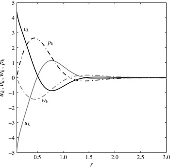
 $$\begin{eqnarray}\boldsymbol{u}^{\prime }=\boldsymbol{u}_{\boldsymbol{k}}(r)\text{e}^{\text{i}kz+\text{i}m{\it\theta}-\text{i}{\it\omega}t}+\text{c.c.}\end{eqnarray}$$
where c.c. is the complex conjugate.
Introducing this form in the Navier–Stokes and density equations (2.1) and linearizing around the base flow leads for
 ${\it\epsilon}=0$
to
 $$\begin{eqnarray}\displaystyle & \displaystyle -\text{i}({\it\omega}-m{\it\Omega})u_{k}-2{\it\Omega}v_{k}=-p_{k}^{\prime }, & \displaystyle\end{eqnarray}$$
 $$\begin{eqnarray}\displaystyle & \displaystyle -\text{i}({\it\omega}-m{\it\Omega})v_{k}+{\it\zeta}u_{k}=\frac{-\text{i}mp_{k}}{r}, & \displaystyle\end{eqnarray}$$
 $$\begin{eqnarray}\displaystyle & \displaystyle -\text{i}({\it\omega}-m{\it\Omega})w_{k}=-\text{i}kp_{k}-{\it\rho}_{k}, & \displaystyle\end{eqnarray}$$
 $$\begin{eqnarray}\displaystyle & \displaystyle \frac{1}{r}\partial (ru_{k})\partial r+\frac{\text{i}m}{r}v_{k}+\text{i}kw_{k}=0, & \displaystyle\end{eqnarray}$$
 $$\begin{eqnarray}\displaystyle & \displaystyle -\text{i}({\it\omega}-m{\it\Omega}){\it\rho}_{k}=\frac{w_{k}}{F_{V}^{2}}. & \displaystyle\end{eqnarray}$$
 ${\it\zeta}=2{\it\Omega}+r{\it\Omega}^{\prime }$
is the vorticity of the axisymmetric vortex. As previously, the equations have been non-dimensionalized by the core size and the inverse of the angular velocity at the centre. Moreover, the density has been non-dimensionalized by
 ${\it\rho}_{0}$
. The calculus is done in the inviscid case, with
 $\mathit{Re}=\infty$
. After some algebra, the velocity and the density can be written as a function of
 $p_{k}$
:
 $$\begin{eqnarray}\displaystyle & \displaystyle u_{k}=\frac{2\text{i}m{\it\Omega}p_{k}/r-\text{i}{\it\omega}p_{k}^{\prime }}{{\it\omega}^{2}-2{\it\Omega}{\it\zeta}}, & \displaystyle\end{eqnarray}$$
 $$\begin{eqnarray}\displaystyle & \displaystyle v_{k}=\frac{m{\it\omega}p_{k}/r-{\it\zeta}p_{k}^{\prime }}{{\it\omega}^{2}-2{\it\Omega}{\it\zeta}}, & \displaystyle\end{eqnarray}$$
 $$\begin{eqnarray}\displaystyle & \displaystyle w_{k}=\frac{k{\it\omega}p_{k}}{{\it\omega}^{2}-F_{V}^{-2}}, & \displaystyle\end{eqnarray}$$
 $$\begin{eqnarray}\displaystyle & \displaystyle {\it\rho}_{k}=\frac{\text{i}kp_{k}}{{\it\omega}^{2}F_{V}^{2}-1}. & \displaystyle\end{eqnarray}$$
Reintroducing these expressions into (A 8d) leads to a differential equation for the pressure
 $p_{k}$
:
 $$\begin{eqnarray}p_{k}^{\prime \prime }+\left(\frac{1}{r}-{\it\Delta}{\it\Delta}^{\prime }\right)p_{k}^{\prime }+\left[\frac{2m}{r{\it\varpi}}\left({\it\Omega}^{\prime }-\frac{{\it\Omega}{\it\Delta}^{\prime }}{{\it\Delta}}\right)-\frac{k^{2}{\it\Delta}}{F_{V}^{-2}-{\it\varpi}^{2}}-\frac{m^{2}}{r^{2}}\right]p_{k}=0\end{eqnarray}$$
where
 ${\it\Delta}(r)={\it\phi}-{\it\varpi}^{2}$
with
 ${\it\varpi}=-{\it\omega}+m{\it\Omega}(r)$
the Doppler shifted frequency and
 ${\it\phi}=(1/r^{3})\partial (r^{4}{\it\Omega}^{2})/\partial r$
the Rayleigh discriminant. In the numerics, the Rayleigh discriminant is equal to
 ${\it\phi}=4\text{e}^{-r^{2}}(1-\text{e}^{-r^{2}})/r^{2}$
. This differential equation can be derived from the differential equation (6) of Billant & Le Dizès (Reference Billant and Le Dizès2009) for
 ${\rm\Psi}=p_{k}/{\it\varpi}$
.
This differential equation is solved numerically by Matlab, using the boundary conditions
 $p_{k}(0)=0$
,
 $p_{k}^{\prime }(0)=1$
. For each frequency
 ${\it\omega}$
, there is a discrete number set of wavenumbers
 $k$
for which the pressure vanishes at infinity. These solutions correspond to the Kelvin modes for this stratified Gaussian vortex. The wavenumbers are found numerically by minimizing the value of the pressure at
 $r=5$
. For
 ${\it\omega}=0$
and
 $m=1$
, the first wavenumber
 $k$
is equal to 2.326 for
 $F_{V}=11.1$
. The solution for the velocity and the pressure are plotted on figure 22 for this Froude number. They are similar to the functions plotted in Eloy & Le Dizès (Reference Eloy and Le Dizès1999) for
 $F_{V}=+\infty$
.
Radial profile of the three velocity components
 $(u_{k},v_{k},w_{k})$
and of the pressure term
 $p_{k}$
obtained for a Kelvin mode characterized by
 $m=1$
,
 $k=2.326$
,
 ${\it\omega}=0$
and for a Froude number
 $F_{V}=11.1$
.
 $u_{k}$
is represented by the grey line,
 $v_{k}$
is represented by the black line,
 $w_{k}$
is represented by the grey dotted line and
 $p_{k}$
is represented by the black dotted line.

In the following, two Kelvin modes will be coupled by the ellipticity. As will be shown in the next section, this is possible for
 $m=\pm 1$
and
 ${\it\omega}=0$
. For each Froude number, the wavenumber
 $k$
is thus sought numerically and the velocity and density of the Kelvin modes are then computed numerically. However, it should be mentioned that the Kelvin modes can only be calculated for small stratifications (large Froude numbers) since the critical points (where
 $F_{V}^{-2}-{\it\varpi}^{2}$
vanishes) get closer to the centre of the vortex at moderate Froude numbers and prevent the numerical integration of the differential equation.
A.3. Triadic resonance of two Kelvin modes
$({\it\epsilon}\neq 0)$

The elliptic instability can be seen as a triadic resonance between two Kelvin modes and the ellipticity: the ellipticity contains a Fourier component of axial wavenumber
 $k=0$
, azimuthal wavenumber
 $m=2$
and a frequency
 ${\it\omega}=0$
which can couple different Kelvin modes via the nonlinear term of the Navier–Stokes equations. The two Kelvin modes are characterized by their axial wavenumbers
 $k_{1}$
and
 $k_{2}$
, azimuthal wavenumber
 $m_{1}$
and
 $m_{2}$
and frequencies
 ${\it\omega}_{1}$
and
 ${\it\omega}_{2}$
. The perturbation is sought as a sum of two Kelvin modes of amplitude
 $A_{1}$
and
 $A_{2}$
which grow slowly in time with a growth rate
 ${\it\epsilon}{\it\sigma}$
:
 $$\begin{eqnarray}\boldsymbol{U}^{\prime }=A_{1}\boldsymbol{V}_{k1}+A_{2}\boldsymbol{V}_{k2}=[A_{1}\boldsymbol{U}_{k1}(r)\text{e}^{\text{i}k_{1}z+\text{i}m_{1}{\it\theta}-\text{i}{\it\omega}_{1}t}+A_{2}\boldsymbol{U}_{k2}(r)\text{e}^{\text{i}k_{2}z+\text{i}m_{2}{\it\theta}-\text{i}{\it\omega}_{2}t}]\text{e}^{{\it\epsilon}{\it\sigma}t}+\text{c.c}.\end{eqnarray}$$
In this section, upper case bold letters
 $\boldsymbol{U}$
correspond to the penta-vector
 $(u,v,w,{\it\rho},p)$
. Moreover,
 $\boldsymbol{U}_{k1}$
and
 $\boldsymbol{U}_{k2}$
are penta-vectors depending only on
 $r$
, whereas
 $\boldsymbol{V}_{k1}$
and
 $\boldsymbol{V}_{k2}$
also contain the axial, azimuthal and temporal dependence. The problem is to determine the growth rate
 ${\it\sigma}$
of the perturbation in the presence of a small elliptic flow
 ${\it\epsilon}\neq 0$
.
Introducing the perturbation (A 14) into the Navier–Stokes equations (2.1) and neglecting the viscous terms and the nonlinear terms
 $A_{1}^{2}$
,
 $A_{2}^{2}$
and
 $A_{1}A_{2}$
leads at first order in
 ${\it\epsilon}$
to:
 $$\begin{eqnarray}\displaystyle {\it\epsilon}{\it\sigma}(A_{1}\boldsymbol{V}_{k_{1}}+A_{2}\boldsymbol{V}_{k_{2}}) & = & \displaystyle -(\boldsymbol{V}_{ell}\boldsymbol{\cdot }\boldsymbol{{\rm\nabla}})A_{2}\boldsymbol{V}_{k_{2}}-A_{2}(\boldsymbol{V}_{k_{2}}\boldsymbol{\cdot }\boldsymbol{{\rm\nabla}})\boldsymbol{V}_{ell}\nonumber\\ \displaystyle & & \displaystyle -\,(\boldsymbol{V}_{ell}\boldsymbol{\cdot }\boldsymbol{{\rm\nabla}})A_{1}\boldsymbol{V}_{k_{1}}-A_{1}(\boldsymbol{V}_{k_{1}}\boldsymbol{\cdot }\boldsymbol{{\rm\nabla}})\boldsymbol{V}_{ell}\end{eqnarray}$$
where
 $\boldsymbol{V}_{ell}={\it\epsilon}(u_{ell},v_{ell},0,0,0)$
is the penta-vector of the elliptic flow.
This linear equation for
 $\boldsymbol{V}_{k1}$
,
 $\boldsymbol{V}_{k2}$
can be written in terms of a matrix
 $\boldsymbol{\mathsf{N}}$
by making
 $\boldsymbol{V}_{ell}$
explicit. It leads to:
 $$\begin{eqnarray}{\it\epsilon}{\it\sigma}(A_{1}\boldsymbol{V}_{k1}+A_{2}\boldsymbol{V}_{k2})={\it\epsilon}(\text{e}^{2\text{i}{\it\theta}}\boldsymbol{\mathsf{N}}_{m_{1}}+\text{e}^{-2\text{i}{\it\theta}}\bar{\boldsymbol{\mathsf{N}}}_{m_{1}})\boldsymbol{V}_{k1}+{\it\epsilon}(\text{e}^{2\text{i}{\it\theta}}\boldsymbol{\mathsf{N}}_{m_{2}}+\text{e}^{-2\text{i}{\it\theta}}\bar{\boldsymbol{\mathsf{N}}}_{m_{2}})\boldsymbol{V}_{k2}\end{eqnarray}$$
where
 $\boldsymbol{\mathsf{N}}_{m}$
is the following matrix:
 $$\begin{eqnarray}\boldsymbol{\mathsf{N}}_{m}=\left(\begin{array}{@{}ccccc@{}}{\it\alpha} & {\it\beta} & 0 & 0 & 0\\ {\it\gamma} & {\it\delta} & 0 & 0 & 0\\ 0 & 0 & {\it\chi} & 0 & 0\\ 0 & 0 & 0 & {\it\chi} & 0\\ 0 & 0 & 0 & 0 & 0\end{array}\right)\end{eqnarray}$$
with
 $$\begin{eqnarray}\left.\begin{array}{@{}l@{}}\displaystyle {\it\alpha}=rf(r)\partial _{r}/2-(rf^{\prime }(r)/2+f(r))m/2+(rf^{\prime }(r)+f(r))/2,\\ \displaystyle {\it\beta}=rf(r)/2\text{i},\\ \displaystyle {\it\gamma}=-[(5r/2-{\it\alpha}r^{2}/2)f^{\prime }(r)+(2-{\it\beta}r^{2}/2)f(r)]/2\text{i},\\ \displaystyle {\it\delta}=-(rf^{\prime }(r)-f(r))/2+rf(r)\partial _{r}/2-(rf^{\prime }(r)/2+f(r))m/2,\\ \displaystyle {\it\chi}=rf(r)\partial _{r}/2-(rf^{\prime }(r)/2+f(r))m/2.\end{array}\right\}\end{eqnarray}$$
There can be a triadic resonance if the term
 $\text{e}^{2\text{i}{\it\theta}}\boldsymbol{\mathsf{N}}_{m_{1}}\boldsymbol{V}_{k1}$
has the same Fourier component as the second Kelvin mode. In this case, the term
 $\text{e}^{-2\text{i}{\it\theta}}\bar{\boldsymbol{\mathsf{N}}}_{m_{2}}\boldsymbol{V}_{k2}$
has the same Fourier component as the first Kelvin mode. There is thus a mutual growth of the two Kelvin modes due to the nonlinear coupling with the ellipticity. The resonance conditions are simply:
 $$\begin{eqnarray}(k_{2}=k_{1},m_{2}=m_{1}+2,{\it\omega}_{2}={\it\omega}_{1}).\end{eqnarray}$$
As previously mentioned, this is obtained for
 $m_{1}=-1$
and
 $m_{2}=1$
with
 ${\it\omega}=0$
due to the symmetry of the dispersion relation of the Kelvin modes. This defines the wavenumber for each Froude number, which is used to compute numerically the profiles of the Kelvin modes.
If the resonance conditions are satisfied, the Fourier component
 $\text{e}^{\text{i}k_{1}z+\text{i}m_{1}{\it\theta}-\text{i}{\it\omega}_{1}t}$
of (A 16) is simply written:
 $$\begin{eqnarray}{\it\epsilon}{\it\sigma}A_{1}\boldsymbol{U}_{k1}=\boldsymbol{\mathsf{N}}_{-1}A_{2}\boldsymbol{U}_{k2}\end{eqnarray}$$
where
 $\boldsymbol{U}_{k1}$
and
 $\boldsymbol{U}_{k2}$
are penta-vectors depending only on
 $r$
. Instead of solving this matrix equation, we define a scalar product:
 $$\begin{eqnarray}\langle \boldsymbol{U}_{i}|\boldsymbol{U}_{j}\rangle =\int _{r=0}^{+\infty }({\bar{u}}_{i}u_{j}+\bar{v}_{i}v_{j}+\bar{w}_{i}w_{j}+F_{v}^{2}\bar{{\it\rho}}_{i}{\it\rho}_{j})r\,\text{d}r\end{eqnarray}$$
for which the linear operator of the Kelvin modes is self-adjoint. Multiplying (A 20) by
 $\langle \boldsymbol{U}_{k_{1}} |$
leads to
 $$\begin{eqnarray}{\it\sigma}A_{1}=N_{12}A_{2}\quad \text{with}\ N_{12}=\frac{\langle \boldsymbol{U}_{k1}|\boldsymbol{\mathsf{N}}\boldsymbol{U}_{k2}\rangle }{\langle \boldsymbol{U}_{k1}|\boldsymbol{U}_{k1}\rangle }.\end{eqnarray}$$
Here
 $N_{12}$
is a simple integral over
 $r$
and can be calculated numerically since the components of the Kelvin modes are known numerically. Doing the same reasoning for the Fourier component of the second Kelvin mode leads to
 $$\begin{eqnarray}{\it\sigma}A_{2}=\bar{N}_{21}A_{1}\quad \text{with}\ \bar{N}_{21}=\frac{\langle \boldsymbol{U}_{k2}|\bar{\boldsymbol{\mathsf{N}}}\boldsymbol{U}_{k1}\rangle }{\langle \boldsymbol{U}_{k2}|\boldsymbol{U}_{k2}\rangle }.\end{eqnarray}$$
Growth rate
 ${\it\sigma}$
of the elliptic instability for a stratified vortex as a function of the Froude number. Circles correspond to the prediction developed in this appendix A using the global approach for a Gaussian vortex, with the first (grey symbols) and second (black symbols) Kelvin mode. The dash-dotted line corresponds to the prediction by Kerswell (Reference Kerswell2002) using a local approach (A 25). Stars correspond to the growth rate (A 26) predicted by Guimbard et al. (Reference Guimbard, Le Dizès, Le Bars, Le Gal and Leblanc2010) using a global approach for the flow inside a cylinder for the first Kelvin mode (grey symbols) and the second Kelvin mode (black symbols).

Multiplying these two equations leads to the value of the growth rate:
 $$\begin{eqnarray}{\it\sigma}=\sqrt{N_{12}\bar{N}_{21}}.\end{eqnarray}$$
It can be calculated numerically for each Froude number by computing
 $N_{12}$
and
 $\bar{N}_{21}$
. This result using the global approach has been plotted on figure 23 as grey disks for the first wavenumber and as black disks for the second wavenumber. The prediction is very close to the result found by Kerswell (Reference Kerswell2002) using a local approach:
 $$\begin{eqnarray}{\it\sigma}_{local}=\frac{9(1-F_{V}^{-2})}{16(4-F_{V}^{-2})}{\it\epsilon},\end{eqnarray}$$
which is plotted as a dash-dotted line. This result tends to
 $9{\it\epsilon}/16$
at large Froude numbers.
The result obtained by Guimbard et al. (Reference Guimbard, Le Dizès, Le Bars, Le Gal and Leblanc2010) using a global approach for the flow inside an elliptic cylinder has also been plotted as stars. The growth rate has an analytic expression given by
 $$\begin{eqnarray}{\it\sigma}_{cylinder}=\frac{9(1-F_{v}^{-2})({\it\varphi}^{2}+1)}{12(2+F_{v}^{-2})+4{\it\varphi}^{2}(4-F_{v}^{-2})}\end{eqnarray}$$
where
 ${\it\varphi}$
is the first (resp. second) root of
 $\text{J}_{0}({\it\varphi})+3\text{J}_{2}({\it\varphi})=0$
for the first (resp. second) Kelvin mode plotted as grey (resp. black) stars. Here,
 $\text{J}$
is the Bessel function.
All the results are very close (within 6 %). Moreover, all the values of the growth rate decrease with the inverse of the Froude number. This indicates that the stratification tends to stabilize the elliptic instability. However, this result is limited to large Froude numbers due to the presence of critical points in the equation of the Kelvin modes. More work would be needed to compute the growth rate at moderate Froude numbers.