Assumptions, Measurement, Performance

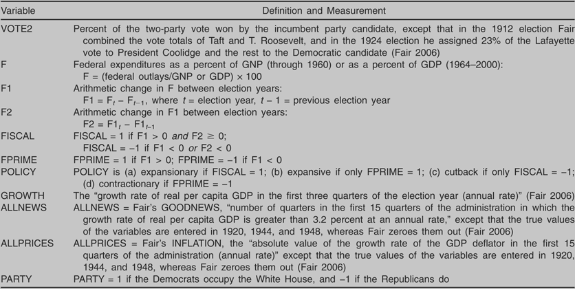
The fiscal model of presidential elections rests on the premise that the share of the two-party vote going to the incumbents, VOTE2, is inversely related to changes in F, the ratio of federal outlays to gross domestic product (GDP).Footnote ¹ (See Table 1 for definitions and measurement of all variables.) Throughout this paper, changes in spending are to be understood in this relative sense. The intuition is that F represents the equivalent of a fee that the federal government charges the polity for its services. As with any commodity, the higher the federal fee, the smaller the quantity demanded. Unlike consumers, however, voters are not able to reduce their purchases from Washington when its fee goes up. Instead, assuming there has been no change in their evaluation of federal goods and services, they do the next best thing. Switching metaphors, on Election Day they “fire” the incumbents. Viewed in this light, an election is equivalent to a retrospective-minded referendum on, ceteris paribus, the president's fiscal policy.

Table 1.

Variable Definitions and Measurements

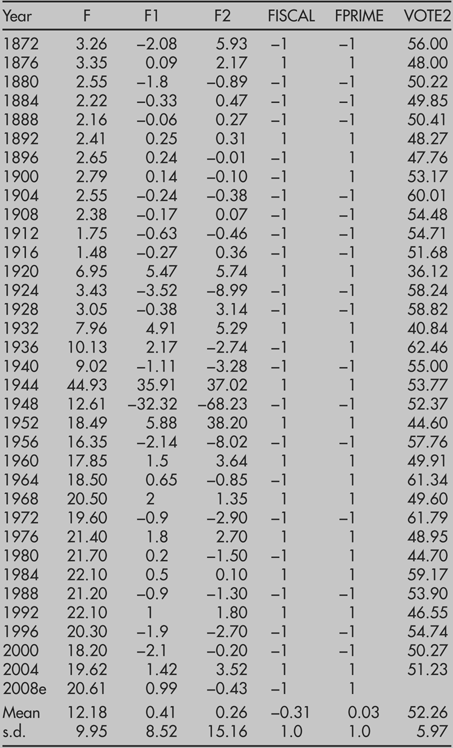
FISCAL, a binary variable derived from the first and second derivative of F (F1 and F2, respectively), captures the direction and rate of change in spending. If FISCAL = 1, policy is expansionary. A cutback policy, signified by FISCAL = −1, indicates either a reduction of expenditures or a deceleration in their rate of growth. By itself, FISCAL turns out to be a powerful predictor of presidential election outcomes. For well over a century, when policy has been cutback, incumbents returned to the White House 85% of the time. By contrast, in 75% of the cases where policy was expansionary, the electorate voted for the opposition party. Omitting 1912, when the Republicans split into two, 80% of all presidential elections held since 1872 behave as expected. Similar results are obtained with FPRIME, a simpler, yet more exacting spending measure. FPRIME is scored 1 if the budget has grown between election years (POLICY is expansive), and −1 if it has shrunk (POLICY is contractionary). Over 90% of incumbents who pursued a contractionary policy won reelection, while only 35% of those implementing an expansive policy did so. (All fiscal data are included in the Appendix.)

Note that the two variables do not always characterize POLICY in the same way. They coincide under two conditions. When FISCAL = 1, so FPRIME = 1, as the former cannot be positive unless the latter is. This means that in the current term the budget has grown at the same or faster rate than in the previous presidential term. Thus, spending has increased unambiguously. Policy is expansionary, and the two variables should have approximately the same impact on election outcome. If FPRIME is negative, this means that spending has actually shrunk; hence, FISCAL is also negative. Policy is contractionary. Again, measured with either variable, the effects on the election should be similar. The discrepancies arise when FPRIME registers a positive change but FISCAL a negative one. This happens whenever the increase in spending during the current term is smaller than in the previous term. Then the characterization of policy, and thus its hypothesized electoral consequences, differs fundamentally, depending on the spending measure. If it is FPRIME, policy is expansive, and the incumbents are predicted to lose; if FISCAL, policy is cutback, and the in-party is anticipated to win. This is because the latter differentiates policy according to the rate of growth in spending, while the former does not. FISCAL embodies the assumption that the electorate rewards a president equally for reducing the rate in spending growth relative to the previous term or for actually slashing the budget. This is why we say that FPRIME is at once simpler and more exacting than FISCAL: it assumes that voters hold the incumbents accountable for budget expansion regardless of its rate of growth. We will return to this difference between the two variables presently, for it makes all the difference in the characterization of policy in the second term of the Bush presidency and, more to the point, the forecast for November.

The relation between POLICY and VOTE2 persists in the presence of four control variables. Three are borrowed from Ray Fair's presidential vote equation: two assaying the state of the economy, GROWTH and ALLNEWS, and DURATION, a weighted index of the number of consecutive terms the incumbents have occupied the White House (Fair Reference Fair2006). The first two are hypothesized to redound to the benefit of the incumbents, and the last to work against them. PARTY is also included, because not only Fair but Alesina and Rosenthal (Reference Alesina and Rosenthal1995) found that Republicans tend to do better than Democrats at the polls.

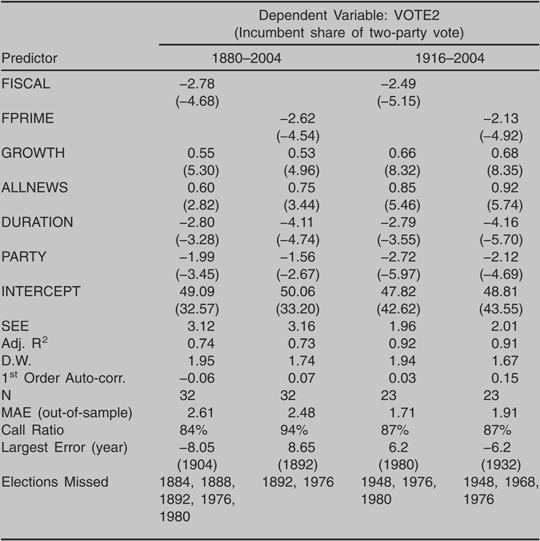
Table 2 displays the fiscal model, combining either FISCAL or FPRIME with the four aforementioned controls, estimated over two different periods, 1880–2004 and 1916–2004. The longer period includes all 32 elections for which Fair provides data. The shorter interval is the one over which Fair estimates his equation and the fiscal model has been calibrated for the purpose of forecasting, as in 2004. Henceforth we will label a fiscal model estimated over the longer period as “long” and one estimated over the shorter period as “short.” In both models, long and short, the coefficients of all variables have the correct sign, and are statistically significant. Note that a switch in policy from cutback to expansionary, or from contractionary to expansive, costs the incumbents approximately 4–5% of the two-party vote (FISCAL and FPRIME range from −1 to 1, so to estimate the impact of either on VOTE2 one multiplies their coefficients by two). Across all models, from 85% to 95% of the out-of-sample elections are called correctly, with a mean absolute error (MAE) of less than 2.0 in the short models, which have a better fit with the data, and less than 3.0 in the long ones.

Table 2.

The Fiscal Model: Two Versions, Two Periods (t-statistics in parenthesis)

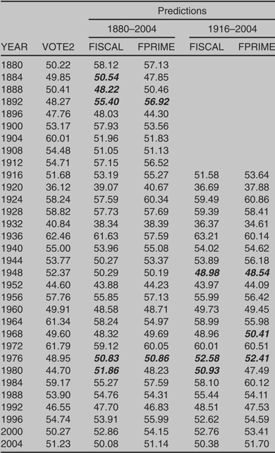
In Table 3 we further explore the performance of both versions of the fiscal model. In out-of-sample forecasting, the two models are in close agreement with themselves between periods, as well and between themselves within periods. The average Pearson's r correlation between any two predictions of VOTE2 is 0.96. The mean absolute difference between the two sets of predictions is 1.57 (s.d. = 1.31) with the long models, and 1.37 (s.d. = 0.96) with the short ones. Also, over 90% of the time the long models coincide in their predictions of the winner (whether or not these calls were made correctly), while the short models do so more than 95% of the time. With so much agreement among the models, one might be tempted to conclude that one is just as good as the other for the purpose of forecasting this year's election. But a closer inspection of the individual errors, particularly of the election outcomes wrongly predicted, the “miscalls,” tells a different story.

Table 3.

Out-of-Sample Predictions of Fiscal Model, by Period and Specification

Note: Miscalls, where the winner is wrongly predicted, are shown in bold italics.

The unshared miscalls of the long models are the predictions for 1884, 1888, and 1980, all of which occurred only with FISCAL in the model. The discrepant errors with the short models are those of 1968, which the model with FPRIME got wrong, and, again, that of 1980, which the model with FISCAL miscalled. All such unshared mistakes but the last concern close elections that one model or the other missed by one or two points. Not so with the 1980 election, the most recent error of any of the models. Short or long, the model with FISCAL called the election for the incumbents, over-predicting President Carter's vote by 6–7 points, whereas in fact he lost badly to Ronald Reagan. Note, too, that this is the largest error of the short model with FISCAL. By contrast, the largest error with its FPRIME sibling fell (harmlessly) on the same side of the election outcome in 1932, where it under-predicted President Hoover's share of the vote, while still correctly calling the election a defeat for the incumbents. Thus, as a practical matter, the 1980 error incurred with the short model with FISCAL is far more serious. In fact, it was a blunder, by which we mean wrongly predicting the winner of an election that was nowhere near close. In this case, the spread between the two presidential candidates was more than 10 points.

Therefore, we conclude that although in terms of the MAE both models with FISCAL perform somewhat better than theirsiblings, when it comes to maximizing the call rate or avoiding blunders, the models with FPRIME are preferable. As we shall see, the 2008 election is one of those rare cases where the models will not share an error: one is predicting a third term for the Republicans and the other a return of the Democrats to the White House. This is the challenge to the fiscal model that gives the title to this paper. To this challenge we now turn.

President Bush's One-of-a-Kind Politico-Fiscal Record

Whether measured by FISCAL or FPRIME, the Bush administration is atypical; in one respect, even unique. Since the 1870s, less than a handful of first-term presidents have implemented an expansionary policy. They are Benjamin Harrison (1892), Herbert Hoover (1932), Ronald Reagan (1984), and George W. Bush. Of these, only Reagan and Bush won reelection. In fact, only Franklin D. Roosevelt managed to win reelection by a like policy—but in his third term, during World War II. Moreover, only three other times has a president won reelection at the end of a term in which POLICY, though cutback as measured by FISCAL, was expansive according to FPRIME: William McKinley (1900), Franklin Roosevelt (1936), and Lyndon Johnson (1964). So in one and a quarter centuries only five presidents have returned to the White House after implementing a policy that was either expansionary or expansive. Of these, two were charismatic (Roosevelt and Reagan), and one was coming up for election in his own right after being elevated to the presidency following the assassination of his predecessor (Johnson), a tragedy that may have elicited public sympathy for the incumbents. Neither condition held for George W. Bush, which may account, at least in part, for his meager victory margin; it was not only much narrower than any of the others, but one of the thinnest on record, the smallest of any other sitting president since Grover Cleveland's in 1888 (when he lost in the Electoral College).

Bush is also atypical in that his is one of only two administrations that pursued an expansive policy (FPRIME = 1) two terms in a row, the previous being the Kennedy-Johnson administration. In fact, the net increase in F over Bush's two terms (estimated at 2.4%) is larger than that of any other presidency since Kennedy-Johnson (2.7%). However, in the case of the latter, the sequence was a cutback policy in the first term (FISCAL = −1), which resulted in a near-record reelection, followed by an expansionary policy in the second term (FISCAL = 1), which ended in defeat. Bush is alone in having done the reverse (FISCAL = 1 in the first term, FISCAL = −1 in the second).

Summing up: President Bush's administration is highly unusual or unique in that (1) he is only one of three presidents to have been reelected at the end of a term of unambiguous fiscal expansion, and only one of two first-term presidents to have done so; (2) his 2004 reelection margin was the second smallest since the present two-party system came into being; (3) his administration is only one of two where policy as measured by FPRIME has been expansive for two consecutive terms; (4) during his presidency, federal spending has grown more than in any other since 1968; and (5) finally and most importantly, although in the term that is coming to an end spending growth has slowed down, describing a cutback policy, it represents a deceleration with respect to his own first term, not to the last term of the previous opposing political party's administration, as in 1900 (McKinley), 1936 (Roosevelt), or 1964 (Johnson).Footnote ² This last fact, especially, makes us doubt whether the fiscal model with policy measured by FISCAL will yield an accurate forecast for 2008.

Choosing a Forecast for 2008

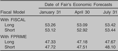
To forecast the outcome of this year's election, we rely on Fair's forecasts of the economic variables, made with his own model of the economy. Taking Fair's January 31, April 30, and July 31 values for GROWTH and ALLNEWS (respectively 1.8 and 2, 1.5 and 2, and 1 and 3), Table 4 displays point predictions of VOTE2 obtained with the fiscal models. The models with FISCAL, short and long, forecast a Republican victory with 53% of the two-party vote, or just under their 1988 showing. By contrast, those with FPRIME forecast approximately the reverse, a Democratic comeback by a margin lying somewhere between their 1976 and 1992 wins. The question then becomes, to which forecast should we attach the greater credence?

Table 4.

2008 Presidential Election Forecasts, by Model and Period

In two sections back, we argued that if the object is to minimize the average error across all elections, one should prefer the models with FISCAL, but if one wishes to avoid a blunder, one should favor the models with FPRIME. Although none of the models forecasts a blowout for either party, they are sufficiently apart so that if one has it about right, the other will turn out to be, if not a blunder, a major error, about the size of the two or three largest incurred by the short models. Having argued in the previous section that due to the atypical and unique nature of the Bush administration, the 2008 forecast of the model with FISCAL is questionable, our desire to avoid a blunder is one reason to go with the forecast issued with the FPRIME version of the model.

Since the fiscal model borrows three variables from Fair, another consideration has to do with what his equation is predicting, for the latter's out-of-sample predictions of VOTE2 correlate strongly with those of both short fiscal models (Pearson's r = 0.84 in each instance). Fair's July 31 forecast is for the Republican candidate to take 48.5% of the two-party vote. This is within a point of that obtained with the fiscal model with FPRIME. Along these lines, it bears noting that in out-of-sample forecasting, Fair's equation misses eight elections, those of 1916, 1948, 1960, 1968, 1976, 1988, 1992, and 2000. Note that all three miscalls made with the short model with FPRIME are included in this set, but in the case of the short model with FISCAL, only two of the three are—the latter's 1980 blunder being the only exception. So this comparison, too, weighs in on the side of the models with FPRIME.

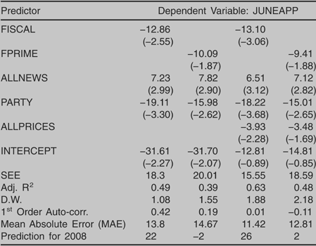
A final aid in making a choice between the two forecasts has to do with the fiscal model's predictions of a variable that is highly correlated with VOTE2, has been used successfully in presidential elections forecasting, and whose value, or at least that of a close substitute, is available four months ahead of the election. That variable is the net presidential approval rating, obtained by subtracting the percent of survey respondents who disapprove of the president's performance from those who approve it in Gallup's final poll in June (available from the Roper Center). This variable, one of three in Abramowitz's “time for change” model, which he calls “JUNEAPP,” alone accounts for about two-thirds of the variance in VOTE2 (Abramowitz Reference Abramowitz2008). Given that a president's approval rating midway through the election year is so closely correlated with the incumbent party's candidate's showing at the polls, it should come as no surprise that, as we have shown elsewhere, a reduced fiscal model that includes FISCAL, ALLNEWS, and PARTY accounts for most of the variation in JUNEAPP (Cuzán and Bundrick Reference Cuzán and Bundrick2006).

In Table 5, columns 2 and 3, we display the results of modeling JUNEAPP with both fiscal models. Neither model has a tight fit with the data, although the one with FISCAL does better in this regard. On the other hand, with this model the Durbin-Watson statistic (DW) is significant for positive autocorrelation. This suggests that there is a missing variable. We know from previous research that changes in the price level are correlated with presidential approval (Erikson, MacKuen, and Stimson Reference Erikson, MacKuen and Stimson2002). Adding ALLPRICES, an inflation measure borrowed from Fair (Reference Fair2006), whose value as of April 30 Fair puts at 3.0, corrects the problem and improves model fit in both models, while hardly disturbing the other coefficients. For the purpose of this paper, though, it is the JUNEAPP forecasts that are of interest. Note that, as with VOTE2, the predictions differ substantially, the pair generated by the model with FISCAL being far rosier for the incumbents than the one with FPRIME. While the former has it as 22 with the uncorrected model and 26 with the corrected model, the corresponding predictions with FPRIME are −2 and 2, respectively.

Table 5.

Predicting Net Presidential Approval (JUNEAPP) with Reduced Fiscal Models, 1948–2008 (t-statistics in parenthesis; N = 15)

In fact, however, the median value of President Bush's net approval rating in the late June polls available at Real Clear Politics is −35. That the actual value of JUNEAPP is closer to the forecasted value generated with the fiscal model with FPRIME is yet another reason to surmise that the forecast for November obtained with this model is to be trusted more.

In conclusion, we will go with the short FPRIME model forecast. Accordingly, we anticipate that the Republicans will lose the White House in a close election, taking about 48% of the two-party vote. The probability that they will take less than 50% is 0.80. Needless to say, our confidence in this forecast would be greater if the corresponding model with FISCAL were in approximate agreement.