




No CrossRef data available.
EFFECTS OF DIFFERENCES IN RISK AVERSION ON THE DISTRIBUTION OF WEALTH
Published online by Cambridge University Press: 01 November 2004
Abstract
This paper studies the role played by differences in risk aversion in affecting the long-run distribution of wealth across agents in the context of an endowment economy. The economy is populated by two types of Epstein-Zin agents who differ only in their attitudes toward risk. By choosing riskier portfolio strategies, less-risk-averse agents enjoy returns on their investments characterized by a higher mean and a higher variance than the ones enjoyed by more-risk-averse agents. The former effect tends to make less-risk-averse agents wealthier over time, whereas the latter tends to make them poorer. The paper shows that, contrary to the results obtained using standard expected utility preferences, for some parameter values the long-run distribution of wealth is dominated by more-risk-averse agents.
Information
- Type
- ARTICLES
- Information
- Copyright
- © 2004 Cambridge University Press
INTRODUCTION
Since at least Ramsey (1928), preference heterogeneity has been recognized as an important determinant of the wealth distribution across individuals. Ramsey (1928, p. 559) conjectured that in a version of the one-sector growth model where dynasties have heterogeneous discount factors, “equilibrium would be attained by a division of society into two classes, the thrifty enjoying bliss and the improvident at the subsistence level.” Becker (1980) verified this conjecture by showing that in a dynamic general equilibrium economy, where the lifetime utility index takes the standard time-additive form with a constant discount factor, the most patient dynasty owns all the capital stock in the long-run steady state.1
Epstein and Hynes (1983) and Lucas and Stokey (1984) consider recursive utility functionals where an agent's discount factor is not constant, but depends on an index of future consumption. They show that in the long-run steady state, more patient households are wealthier, but, differently from Becker (1980), all households own positive amounts of capital.
Little attention has instead been paid to the relationship between attitudes toward risk and the distribution of wealth. In the standard expected utility framework, attitudes toward risk aversion cannot be disentangled from attitudes toward intertemporal substitution, making it impossible to pin down the effect of differences in risk aversion on the wealth distribution.2
It is well known that within the standard expected utility framework with complete markets, the less-risk-averse agent dominates the wealth distribution in the long run if the economy is growing over time [see Dumas (1989) and Wang (1996)]. This result holds in deterministic as well as in stochastic settings, suggesting that risk considerations do not play a role in generating it.
A class of preferences that allows for such separation has been introduced by Epstein and Zin (1989). Commenting on the advantages of their recursive preferences, Epstein and Zin (1989, p. 960) emphasize that “the separation which they provide should make them useful in exploring the role played by differences in risk aversion in influencing the distribution of wealth across agents.” This exploration is the objective of this paper. The approach I take is to analyze the dynamics of the wealth distribution in a simple endowment economy populated by two types of Epstein-Zin agents with different degrees of risk aversion but the same intertemporal elasticity of substitution.3
Anderson (1998) considers the dynamics of efficient allocations in complete-markets economies where agents have recursive preferences. However, he does not consider the case of Epstein-Zin agents with different degrees of risk aversion.
The main result of the analysis is that, differently from models based on expected utility, the share of wealth owned by agents with higher risk aversion does not necessarily tend to shrink over time. When attitudes toward risk are separated from attitudes toward intertemporal substitutability, there are parameter values for which more-risk-averse agents always dominate the long-run distribution of wealth. This apparently counterintuitive result is due to the fact that the dynamics of the wealth distribution are not only determined by the first moment of the rate of return on the agents' portfolios, but also by the second moment. Thus, although less-risk-averse agents, by exploiting the equity premium to their advantage, tend on average to earn a higher return on their savings, they also pursue riskier portfolio strategies which may, in fact, lead them to lose all their wealth in the long run.
The rest of the paper has the following structure. Section 2 introduces the notation and the model. Section 3 discusses the dynamics of the wealth distribution. Section 4 concludes.
THE ECONOMY
In this section, I introduce a simple endowment economy populated by two types of Epstein-Zin agents who differ only in their degree of risk aversion. I consider two alternative structures for the asset market. In the first one, the asset market is complete, whereas in the second one a borrowing constraint limits the scope for risk sharing between agents. In the former case, the long-run distribution of wealth in the economy is always degenerate. According to the parameters of the model either the more- or the less-risk-averse type of agent dominates the distribution of wealth. In the latter case, instead, the long-run distribution of wealth in the economy may be stationary. Even in this circumstance though, the distribution of wealth can be concentrated in the hands of more-risk-averse agents.
Preferences
The economy is populated by two types of agents, individually denoted by i=1,2. The size of each type is normalized to 1. Denoting by Uit agent i's utility from time t onward, the preferences of each agent are represented by the following recursive utility function4
The expression for the utility function when ρ=0 (unit intertemporal elasticity of substitution) is easily obtained using de l'Hospital's rule to compute the limit of
for ρ→0. Tallarini (2000) considers the case of unit intertemporal elasticity using Epstein-Zin preferences in a real-business-cycle representative-agent model.

where β is the discount factor, Et[·] denotes the expectation conditional on information available at the beginning of time t, and Cit denotes consumption by an agent of type i at time t. These preferences have been introduced by Epstein and Zin (1989) to allow for the independent parameterization of an agent's attitudes toward intertemporal substitution and his degree of risk aversion. In this specification, (1-ρ)−1 is the elasticity of intertemporal substitution and γi<1 parameterizes risk aversion, with higher values of γi denoting lower risk aversion.5
These preferences have been extensively used in the asset pricing literature. See, for example, Epstein (1988), Weil (1989), Epstein and Zin (1991), and Campbell (1993). Epstein and Zin (1989, pp. 949–950) discuss the interpretation of the parameters ρ and γi.
To evaluate the effects of heterogeneity in risk aversion, I assume that the agents in this economy share the same intertemporal elasticity parameter ρ and have different degrees of risk aversion. By convention, agents of type 1 are more risk averse than agents of type 2: γ1<γ2.
In the following, I focus on the case of unit intertemporal elasticity of substitution (ρ=0). This assumption simplifies the interpretation of the results because it implies that agents with different risk aversion have the same propensity to save out of current wealth. Therefore, the dynamics of the wealth distribution are entirely driven by their different portfolio choices. The main results of the paper easily generalize to the case of elasticity of substitution different from one.6
The results for the case ρ≠0 are available from the author upon request.
Endowment
The aggregate endowment, in each period, consists of a perishable dividend Dt. This evolves according to the process

The growth rate λt+1 follows an i.i.d. two-state Markov process
with
and Pr
Markets and Assets
At each point in time, there exists a spot market for the consumption good, which I take to be the numeraire, a market for a one-period riskless asset (“bond”), and a market for a risky asset (“stock”) that pays the dividend Dt at time t. I denote by Bit the quantity of bonds held by agent i at the beginning of time t and by qt their price in terms of the consumption good. For convenience, I also define bit+1 to be the ratio
.
I denote by sit the share of the stock held by agent i at the beginning of time t and by Pt the ex-dividend price of one share in terms of the consumption good. I also denote by
the stock price dividend ratio. The total number of shares outstanding is normalized to 1.
Budget and Borrowing Constraint
Both types of agents maximize their time-zero utility Ui0 subject to the sequence of budget constraints

where cit denotes the ratio
. Without loss of generality, I assume that at time zero,
and
.
In addition to this frictionless complete-markets economy, I also evaluate the effects of borrowing constraints on the long-run distribution of wealth. In particular, to keep the analysis simple, I consider situations where an agent has to finance a fraction κ<1 of his stocks' purchase out of his own savings7
This constraint can be interpreted as a margin requirement. It simplifies the analysis with respect to a constraint of the type
for some constant
because it implies, with the homotheticity of preferences, that decision rules are linear in agents' wealth. See the agent's optimization problem and Coen-Pirani (in press) for details.

Recursive Formulation and Equilibrium
In this economy, aggregate demand for assets and the consumption good, as well as the bond price, depend, in general, on the way aggregate wealth is distributed across agents. Let
denote the fraction of aggregate wealth, 1+pt, held by the more-risk-averse type of agent at time t:

The law of motion for Γt, which summarizes the state of the economy at the beginning of period t, is denoted by

This function relates the distribution of wealth at time t+1 to the current state and the realization of the endowment shock λt+1.
Letting w represent individual wealth, appropriately standardized by D, homotheticity of preferences implies that the agents' problem can be written recursively as follows:


The definition of recursive equilibrium for this economy is standard, requiring individual optimization and market clearing. The only feature of this definition that is worth noticing is the fact that in equilibrium the perceived law of motion for the distribution of wealth H(Γ,λ′) must be consistent with agents′ behavior:

Notice that the first argument of the stock and bond demand functions s1′(.,.) and b1′(.,.) in equation (4) is type-1 agents' wealth in equilibrium, while the second argument is the aggregate state of the economy Γ.
Agents' Optimization Problem
Homotheticity of preferences and the linearity of the budget and borrowing constraints imply that the value function for both types of agents and the decision rules for consumption and asset holdings can be written as the product of individual wealth w and a term involving only the distribution of wealth Γ. For example, the value function and the decision rule for consumption take, respectively, the form
and
for some positive functions
and
.
Moreover, the optimization problem in (3) can be recast in a consumption-savings problem and a portfolio decision problem. To do this, denote the fraction of an agent's savings invested in stock by
and the rate of return on his portfolio by

where the rate of return on the risky and riskless assets are, respectively,

An agent's next-period wealth can then be rewritten as

while, using the definition of x, the borrowing constraint (2) amounts to
.
Taking into account the linearity of the value function and of the decision rules in w, the recursive problem (3) becomes

As it is clear from equation (6), the consumption-savings decision can be analyzed independently from the portfolio choice problem. The assumption of unit elasticity of substitution implies that in every state Γ, an agent of type i chooses to consume a fraction
of his wealth, independently of his degree of risk aversion. Thus, in this case the dynamics of the wealth distribution are driven exclusively by the different portfolio decisions made by the agents. Moreover, their common propensity to save out of wealth implies that the stock price dividend ratio p(Γ) is a constant equal to
This can be seen by imposing the market-clearing condition for consumption,

and solving for p(Γ). The rate of return on stocks is therefore
which simplifies to λ′β since p(Γ)=β/(1–β).
DYNAMICS OF THE DISTRIBUTION OF WEALTH
In this section, I study the dynamics of the wealth distribution in this economy. I am particularly interested in exploring the robustness of the standard result, derived within the expected-utility framework, according to which less-risk-averse agents always tend to dominate the long-run distribution of wealth if the economy is growing.
The focus of the analysis is represented by the equilibrium law of motion for the distribution of wealth
Using the notation introduced in the preceding section, it is easy to see that

Notice that the mapping
has only two fixed points:
and
If
type-2 agents own all the wealth in the economy, whereas the opposite occurs at
. Taking logarithms, the law of motion for the wealth distribution (7) can be rewritten as

where the innovation
is defined as

and by construction has a conditional mean equal to zero. Equation (8) suggests that the share of wealth of type-2 agents will tend to grow, on average, as long as the conditional expectation term is positive or, equivalently, if

Equation (9) contains the key to understanding why in the long run less-risk-averse agents may tend to become poorer and poorer. The term on the left-hand side of this equation is the expected value of the logarithmic return on type-2 agents' portfolio. The term on the right-hand side is the logarithm of the rate of return on a portfolio that contains only stock. The fact that less-risk-averse agents are levered and therefore choose portfolios where stocks receive a weight larger than 1
implies that, on average, the rate of return on their portfolio exceeds the rate of return on stock:

However, levered portfolios are also riskier. The concave transformation of returns operated by the logarithm implies that equation (9) may not be satisfied, even if equation (10) is. In other words, the share of aggregate wealth owned by type-2 agents may shrink over time, even if their portfolio pays, on average, a higher return than the one on stock. This is the basic intuition behind the fact that less-risk-averse agents may lose all their wealth in the long run in this kind of model.
The main difference with respect to the standard expected-utility framework is that in the latter, less-risk-averse agents also have a higher propensity to save out of current wealth, due to the higher intertemporal elasticity of substitution. In turn, a higher propensity to save increases the growth rate of their wealth with respect to more-risk-averse agents, leading them to become richer and richer over time. Epstein-Zin preferences, instead, allow attitudes toward risk to be parameterized separately from attitudes toward intertemporal substitution. As a result, in this economy the dynamics of the wealth distribution are exclusively driven by the different portfolio choices made by the agents.
Of course, even if type-2 agents' portfolios are riskier, I have not shown yet that this effect can be strong enough to lead them to lose all their wealth in the long run. Since the model does not admit an analytical solution, I proceed in two complementary ways. First, I evaluate the conditional expectation on the left-hand side of equation (9) at the steady state Γ=1. Second, I solve the model numerically and verify that the dynamics of the wealth distribution around Γ=1 are in fact consistent with the intuition obtained at Γ=1.
Consider the first approach. The inequality (9) evaluated at the steady state Γ=1 determines the stability of the mapping
at Γ=1. That is, it determines whether the share of wealth owned by type-2 agents tends to decline or increase over time in a neighborhood of Γ=1. The conditional expectation on the left-hand side of equation (9) at Γ=1 depends on type-2 agents' portfolio decision x2(1) and the bond return Rb(1). Notice that at the steady state, Γ=1 type-2 agents own zero wealth and therefore save zero and buy zero stock.9
The steady state Γ=1 is never reached by the agents in finite time. To consider the case Γ=1, I endow type-2 agents with zero wealth.
Both Rb(1) and x2(1) can be computed analytically. The return Rb(1) is simply the rate of return on one-period bonds in a representative-agent economy populated only by type-1 agents. The portfolio decision x2(1) is found by solving the optimization problem (6) at Γ=1.10
In particular, it can be easily shown that

Notice that, as remarked in note 8,
for all values of Γ ∈[ 0,1]. Weil (1989) analyzes asset prices in a representative-agent economy with Epstein-Zin preferences. The analytical expression for x2(1) is obtained from equation (A.2) in the Appendix by setting Γ=1 and noticing that the terms involving the value function υi(·) cancel out since

where
The term in z on the left-hand side of this equation represents the difference between the expected logarithmic return on type-2 agents' portfolio and the expected logarithmic return on stock. The direction of the inequality depends only on whether this term is positive or negative. After some simplifications, one obtains that it is positive if and only if

Thus, these computations suggest that it is in fact possible that inequality (9) is not satisfied so that a riskier portfolio strategy may lead less-risk-averse agents to become poorer and poorer in a neighborhood of Γ=1. This circumstance is more likely to occur [i.e., condition (11) is less likely to be satisfied] the less risk averse agents of type-2 are. Lower risk aversion, in fact, leads to the choice of riskier portfolios, decreasing the growth rate of their wealth. Condition (11) also depends on the degree of risk aversion of type-1 agents because the latter determine the rate of return of the riskless asset. In particular, the less risk averse type-1 agents are (the higher γ1 is), the higher the riskless rate must be to reduce their incentive to sell riskless debt. In turn, a high riskless return reduces the rate of return on type-2 agents' portfolio. Therefore, the higher γ1, the more likely it is that type-2 agents tend to become poorer and poorer when Γ is close to 1.
Repeating the same analysis at Γ=0, one obtains that condition (11) is also necessary and sufficient to guarantee that the share of wealth held by type-1 agents tends to decrease over time in a neighborhood of Γ=0. Therefore, this approach suggests that the long-run distribution of wealth in this economy under complete markets is always degenerate. If condition (11) is satisfied, type-2 agents dominate the long-run distribution of wealth. Conversely, if condition (11) is not satisfied, the long-run distribution of wealth is dominated by type-1 agents.
To confirm these intuitions and to consider the dynamics of the wealth distribution away from the rest points Γ=1 and Γ=0, it is necessary to use numerical methods and assign numerical values to the parameters of the model.11
A description of the numerical algorithm is provided in the Appendix.
Notice that in this calibration the average growth rate of the economy is positive. In the standard expected utility framework of Wang (1996), this would lead less-risk-averse agents to disappear from the economy in the long run. It is important to notice that the exact values of the parameters β, λl and λh are not important for the long-run dynamics of the wealth distribution, since, as equation (11) suggests, the key parameters are γ1 and γ2.

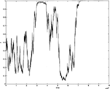
I first consider the complete-markets version of the model, without the borrowing constraint (2). Figure 1 shows the dynamics of Γt when the two types have risk aversion parameters γ1=−0.1 and γ2=0.3, so that condition (11) is not verified. The figure shows how the process Γt eventually converges to 1; that is, the more-risk-averse type dominates the long-run distribution of wealth. It is important to stress the fact that {Γt} converges to 1 only asymptotically.13
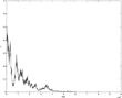
In Figures 1 and 2, convergence occurs in finite time because the precision of the machine used to generate the figures is limited to 16 decimal places.
0.01, and satisfy condition (11).

More-risk-averse agents dominate the long-run distribution of wealth.

Less-risk-averse agents dominate the long-run distribution of wealth.
As discussed above, the intuition that explains why type-2 agents can lose all their wealth in the long run has to do with the fact that their portfolio choices are relatively risky. This suggests that introducing an upper bound on leverage and therefore reducing the riskiness of their portfolios may prevent this extreme result from occurring, leading to a stationary long-run distribution of wealth.
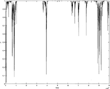
Figure 3 represents the dynamics of the wealth distribution when the parameters are the same as in Figure 1, with the exception of κ, which is set equal to 0.84, so that at Γ=1, the borrowing constraint is binding for agents of type-2: x2(1)=1κ. The introduction of the borrowing constraint is enough to make the growth rate of type-2 agents' wealth positive in a neighborhood of Γ=1. The figure shows how the distribution of wealth does not converge to Γ=1. The process Γt gets extremely close to 1 but always bounces back.

Dynamics of the wealth distribution in the economy with binding borrowing constraints.
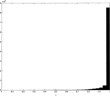
The introduction of this borrowing constraint, while giving rise to a stationary distribution of wealth, does not qualitatively affect the main result of the paper. Figure 4 is a histogram of the wealth distribution corresponding to the simulation of Figure 3. The long-run distribution of wealth is still very much concentrated in the hands of the more-risk-averse agent, because risky portfolio strategies induce less-risk-averse agents to remain poor over time.

Histogram of the stationary distribution of wealth in theeconomy with binding borrowing constraints
SUMMARY
This paper has explored the role played by differences in risk aversion in affecting the long-run distribution of wealth across agents. To disentangle risk aversion from intertemporal substitution I have adopted the recursive preferences introduced by Epstein and Zin (1989). According to the parameters of the model, the long-run distribution of wealth is dominated by either less- or more-risk-averse agents. By choosing riskier portfolio strategies, less-risk-averse agents enjoy returns on their investments characterized by a higher mean and a higher variance than the ones enjoyed by more-risk-averse agents. The former effect tends to make less-risk-averse agents wealthier over time, whereas the latter tends to make them poorer. The paper shows how, differently from a model based on expected utility, the latter effect prevails for some parameter values. Therefore, it is possible that agents characterized by higher risk aversion dominate the long-run distribution of wealth.
APPENDIX: NUMERICAL ALGORITHM
In what follows, I describe in detail the numerical algorithm I have used to first solve and then simulate the model.
SOLVING THE MODEL
The numerical solution of the model features three main steps described below.
Step 1. Solving the Agents' Problem. Solving the agents' problem involves solving the recursive equation (6) to obtain the function υi(Γ), i=1,2, for given initial guesses for\ the functions q(·) and H(.,.) [as observed in the main text the stock price dividend ratio p(Γ) is always equal to β/(1-β)]. The consumption-savings decision and the portfolio choice problem can be solved for analytically, and so, no maximization routine is needed at this step. In particular, analytically solving the maximization problem in equation (6), it is easy to see that the propensity to consume out of wealth is

The portfolio decision of an agent of type i=1,2 is instead

where
is the optimal portfolio choice in the absence of portfolio constraints. Specifically, the unconstrained maximization of equation (6) with respect to x yields

where

I therefore solve equation (6) by replacing the optimal decision rules (A.1) and (A.2) into the Bellman equation (6) and by iterating on υi(·) until convergence. To iterate on (6), I discretize the state space (the unit interval [0,1]) for Γ and construct a grid
using K=200 evenly spaced grid points, with Γ1=0 and Γ200=1. Since, in general, Γ′=H(Γk,λ′) does not lie on the grid, I approximate υi(Γ′) using cubic splines, which produce a twice continuously differentiable interpolated function [see Press et al. (1996, Ch. 3)]. Convergence of the value function υi(Γ) is reached when the maximum (across grid points) percentage difference between the value function at two successive iterations is smaller than 10−7.
Step 2. Finding the Market-Clearing Bonds' Pricing Function. The second step of the algorithm is to use the bond demand functions
produced by step 1 to update the pricing function q(·) at the grid points
Since there are K grid points, this amounts to solving a system of K equations, corresponding to the market-clearing conditions for the riskless asset at each Γk on the grid:

The K unknowns in this system of equations are the bond prices
. To solve this problem, I use Broyden's algorithm, which operates in the following way [for a more detailed description, see Press et al. (1996, Ch. 9)]. First, it numerically approximates the Jacobian matrix associated with the nonlinear system. It then uses this approximate Jacobian to find an updated vector of prices by implementing the Newton step, which guarantees quadratic convergence if the initial guess is close to the solution. If the Newton step is not “successful,” the algorithm tries a smaller step by backtracking along the Newton dimension. When an acceptable step is determined, prices are updated and the algorithm can proceed in the way described above, once an updated Jacobian has been obtained. Since the numerical computation of the Jacobian can be costly (and in this model it is), the Jacobian at the new prices is iteratively approximated using Broyden's formula. The nonlinear solver stops when the maximum excess demand divided by total asset demand is smaller than 10−4. Notice that every time the algorithm tries a different price vector, it has to go back to step 1 and recompute the agents' decision rules in order to evaluate the excess demands at those prices.
Step 3. Updating the Law of Motion for the Wealth Distribution. The third step consists of updating the law of motion for the distribution of wealth H(Γ,λ′) at the grid points
That is, given the law of motion
found at the jth iteration on step 3, use equation (4) to find
:

where, as noted above,

After
has been computed, the algorithm goes back to step 1 with a new law of motion for the wealth distribution. The algorithm stops when the convergence criteria for steps 1 and 2 have been satisfied and the maximum distance (across grid points) between two successive laws of motion for the distribution of wealth is smaller than 10−5.
SIMULATING THE MODEL
The numerical solution of the model yields the equilibrium law of motion for the wealth distribution. The latter is a vector of dimension 200×2:
where
denotes the 200 grid points for the distribution of wealth. Figures 1–4 are generated using data obtained by iterating on the recursion
starting from
which is a grid point. Notice that the number
in general does not belong to the grid
Therefore, to compute
one needs to interpolate the law of motion H(.,λ2) to be able to evaluate it at the point Γ1. Interpolation occurs by means of cubic splines. Cubic spline interpolation has the property that the interpolating function
coincides with the equilibrium law of motion H(Γ,λ′) at the grid points
Moreover, the function
which is defined for all Γ ∈ [0,1],$ is also smooth in the sense that is twice continuously differentiable everywhere. The simulation therefore proceeds using the interpolating function $
to obtain Γt+1 given Γt.
This paper builds on material from my Ph.D. dissertation at the University of Rochester. Thanks to Larry Epstein, Per Krusell (my advisor), Dmitry Kramkov, Marla Ripoll, Alan Scheller-Wolf, Isaac Sonin, Tony Smith, and two anonymous referees for useful comments and suggestions. The usual disclaimer applies.
References
Anderson E.
1998
Uncertainty and the Dynamics of Pareto Optimal Allocations.
Mimeo,
University of Northern Carolina.
Becker R.
1980
On the long-run steady state in a simple dynamic model of equilibrium with heterogeneous households.
Quarterly Journal of Economics
95,
375–
382.Google Scholar
Campbell J.
1993
Intertemporal asset pricing without consumption data.
American Economic Review
83,
487–
512.Google Scholar
Coen-Pirani D.
(in press)
Margin requirements and equilibrium asset prices.
Journal of Monetary Economics.
Dumas B.
1989
Two-person dynamic equilibrium in the capital market.
Review of Financial Studies
2,
157–
188.Google Scholar
Epstein L.
1988
Risk aversion and asset prices.
Journal of Monetary Economics
22,
179–
192.Google Scholar
Epstein L. &
A. Hynes
1983
The rate of time preference and dynamic economic analysis.
Journal of Political Economy
91,
611–
635.Google Scholar
Epstein L. &
S. Zin
1989
Substitution, risk aversion, and the temporal behavior of consumption and asset returns: A theoretical framework.
Econometrica
57,
937–
969.Google Scholar
Epstein L. &
S. Zin
1991
Substitution, risk aversion and the temporal behavior of consumption and asset returns: An empirical analysis.
Journal of Political Economy
99,
263–
286.Google Scholar
Lucas R. &
N. Stokey
1984
Optimal growth with many consumers.
Journal of Economic Theory
32,
139–
171.Google Scholar
Press W.,
S. Teukolsky,
W. Vetterling, &
B. Flannery
1996
Numerical Recipes in Fortran 77: The Art of Scientific Computing.
Cambridge, UK:
Cambridge University Press.
Tallarini T.
2000
Risk-sensitive real business cycles.
Journal of Monetary Economics
45,
507–
532.Google Scholar
Wang J.
1996
The term structure of interest rates in a pure exchange economy with heterogeneous investors.
Journal of Financial Economics
41,
75–
110.Google Scholar
Weil P.
1989
The equity premium puzzle and the risk-free rate puzzle.
Journal of Monetary Economics
24,
401–
421.Google Scholar
More-risk-averse agents dominate the long-run distribution of wealth.
Less-risk-averse agents dominate the long-run distribution of wealth.
Dynamics of the wealth distribution in the economy with binding borrowing constraints.
Histogram of the stationary distribution of wealth in theeconomy with binding borrowing constraints
 You have
Access
- 17
- Cited by