





1 Introduction
A coupled delay-algebraic system was recently introduced and analyzed in [Reference Cheng and Wu12, Reference Zhang, Scarabel, Murty and Wu39] to explore sources of multiple outbreak oscillations of COVID-19 and other emerging infectious diseases reported globally [Reference Ulrichs, Rolland, Wu, Nunes, El Guerche-Séblain and Chit37]. These sources stem from a combination of community’s plasticity for behavioral changes in response to perceived risk and public health capacity to disseminate infection risk information and implement collective decision guided by behavioral changes in a timely fashion during the acute phase and post-acute phase of a pandemic. The two modeling studies considered the onset of Hopf bifurcations of periodic solutions, and the impact of actionable model parameters on the amplitude and frequency of bifurcated periodic solutions. However, both studies focused on local dynamics, including the existence of disease-established and behavior-balanced equilibrium and the occurrence of local Hopf bifurcations of periodic oscillations when the community’s plasticity and public health policy implementation delay are in a small neighborhood of certain critical values calculated from the linearized system of the model at a disease-establishment state. It remains to be an important question to determine if the claimed periodic waves from linearization persist when the aforementioned parameters move away from the critical values. Our objective in this article is to provide some answers to this question, by developing a framework and some techniques based on the equivalent-degree and global Hopf bifurcation theory for a general coupled system of delay differential and algebraic equations.
Delay-algebraic systems were used in conjunction with the concept of infection index that depends either on the past prevalence or incidence in epidemic modeling. This information index approach of the delayed impact of infection risk on the current information to inform behavioral change can also be described by a continuous memory kernel (hence, delay-integral equations may be more appropriate; see [Reference Andó, De Reggi, Scarabel, Vermiglio and Wu1, Reference Bulai, Montefusco and Pedersen5–Reference Buonomo, Messina, Panico and Vecchio10, Reference d’Onofrio and Manfredi15–Reference d’Onofrio, Manfredi and Salinelli19]). Delay-algebraic systems arise also naturally from the study of structured population dynamics, where the population is structured by age with individuals competing for resources to reach maturity [Reference Kosovalić, Chen and Wu26, Reference Magpantay, Kosovalić and Wu30]. Other areas where delay-algebraic systems have been used include path control, electrical design, fluid dynamics, multibody system, and chemically reacting systems (see [Reference Brayton4, Reference Gibbs, Hopf, Kaplan and Shoemaker22, Reference Ikeda, Daido and Akimoto25, Reference Milton, Cabrera, Ohira, Tajima, Tonosaki, Eurich and Campbell32–Reference Shampine and Gahinet35] and the reference therein). In general, delay-algebraic systems resemble both delay differential systems and algebraic (or integral) systems, but it is the hybrid nature of such systems that imposes significant challenges for the qualitative study of dynamic behaviors. Despite the challenges, there are some developed numerical methods [Reference Ascher and Petzold2, Reference Tian, Yu and Kuang36] and qualitative analyses of linear delay-algebraic systems or some particular delay-algebraic systems [Reference Michiels31, Reference Zhu and Petzold40, Reference Zhu and Petzold41] including semi-explicit Hessenberg system) [Reference Campbell and Linh11, Reference Du, Linh, Mehrmann and Thuan20, Reference Luzyanina and Roose29]. The local stability of periodic solutions to semi-explicit index-1 and index-2 delay-algebraic systems has been discussed in [Reference Luzyanina and Roose29] and in [Reference Michiels31] that considered the spectral properties of linear delay-algebraic systems and invented a numerical method for computing characteristic roots, thereby demonstrating the impact of small delay perturbations. The work [Reference Du, Linh, Mehrmann and Thuan20] also discussed the stability of linear delay-algebraic systems and examined the spectral condition for exponential stability. However, to our knowledge, no prior work on global dynamics and global Hopf bifurcation has been reported for this generally hybrid system of delay-algebraic systems.
Here, we develop a general
$S^1$
 -degree theoretic global Hopf bifurcation theory for the following semi-explicit neutral index-1 delay-algebraic system [Reference Ascher and Petzold2],

that is, particularly illustrated by the Zhang–Scarabel–Murty–Wu outbreak model [Reference Zhang, Scarabel, Murty and Wu39] and its extension for the post-outbreak phase [Reference Cheng and Wu12]:

The linear function
$g(x)=g_1(x):=x$
 corresponds to the case where the susceptible population remains relatively unchanged at the early stage of a pandemic, while the nonlinear function
$g(x) =g_2(x):= x(1 - x/N)$
 is more appropriate post the pandemic, when susceptible populations are depleted due to infection and recovery with immunity.
We will, in Section 2, establish the general setting to transform such a delay-algebraic system into a system of delay differential equations with infinitely many delays
$k\tau $
 for all
$k=0, 1, 2,\ldots $
 (at least for solutions of the delay-algebraic system which are defined for all
$t\in R$
 ). This transformation allows us to apply the previously developed global Hopf bifurcation theory for delay equations with infinite delay and two parameters to establish a parallel global Hopf bifurcation theory for delay-algebraic systems. We then develop the necessary techniques for us to apply this global Hopf bifurcation to examine the global continua of slowly oscillating periodic solutions (periodic solutions with period larger than
$2\tau $
 ) and fast oscillations (periodic solutions with period less than
$\tau $
 ) emerging from local Hopf bifurcation of the specific delay algebraic systems from epidemic modeling. In particular, in Section 3, we derive the equivalent cyclic system of ordinary differential equations (ODEs) for periodic solutions of delay-algebraic systems with periods that are integer multiples of the delay. We will analyze properties of such a cyclic system of ODEs in order to rule out periodic solutions, which can then be used to establish the a priori bounds of periods of the periodic solutions along a global continuation of Hopf bifurcations in the Fuller space. In Section 4, we consider the Zhang–Scarabel–Murty–Wu outbreak model as a case study to illustrate the application of our approach. In the final discussion section, we present numerical simulations to illustrate distinctions between our considered delay-algebraic system and a general scalar delay differential equation with a single delay. These distinctions include the unboundedness of periodic solutions with varying time lags as well as the competitive nature with embedded predator–prey interactions of the corresponding cyclic systems of ODEs.
2 The basic setting
2.1 Equivalence to a functional differential equation with infinite delay
In what follows, we consider the following delay differential-algebraic system:

where we assume:
-
(H1) $g: \mathbb {R}_{+}\to \mathbb {R}_{+}$
 is
$\mathbb {C}^2$
-smooth;
-
(H2) $f:\mathbb {R}_+^2\to \mathbb {R}_+$
is given by
$f(x, y)=F(xy)$
, where
$F:\mathbb {R}_{+}\to \mathbb {R}_{+}$
is
$\mathbb {C}^2$
-smooth,
$F(\xi )$
is strictly decreasing on behavioral adaption of incidence
$\xi \geq 0$
with
$F(\infty ):=\lim _{\xi \to \infty }F(\xi )\geq 0$
and
$F(0):=\beta _c>0$
.
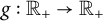

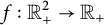






Assumption (H2), more explicitly, the multiplicative assumption on f, is motivated by the epidemic models in [Reference Cheng and Wu12, Reference Zhang, Scarabel, Murty and Wu39], where the incidence rate depends on the product of the transmission rate and the infectivity term. Although some of the principal techniques we developed, such as the reduction of the delay differential-algebraic system to a delay differential equation with infinite delay (for solutions defined for all t), can be applied to general system (2.1) without this multiplicative structure imposed on f, much of the analysis and calculations we present below to exclude periodic solutions with a certain period is detailed with this particular form of f in mind for the sake of simplicity.
Examples arising from the aforementioned studies on disease outbreaks include the linear function

during the early phase of a pandemic [Reference Zhang, Scarabel, Murty and Wu39], with susceptible populations remaining constant; and the quadratic function

post a pandemic [Reference Cheng and Wu12], where
$N>0$
 is a constant for the total population and susceptibility in populations will decrease due to infection-generated immunity. The second component of the coupled system describes the adaptation behavior to the perceived risk of infection of the incidence term
$\beta (t-\tau )g(I(t-\tau ))$
 with
$\tau>0$
 being the sum of the delay from exposure to infection to perception of risk and behavioral changes. The monotonicity assumption in (H2) reflects the reduction of transmission effective contact when the perceived risk increases. Assumption (H1) is clearly satisfied by
$g_1$
 and
$g_2$
 .
An equilibrium
$E^*=(I^*, \beta ^*)$
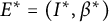 of the coupled system is given by

It is obvious that if
$g(I^*)$
 is given, then
$\beta ^*$
 is a fixed point of
$f(\beta ^*, g(I^*))$
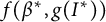 . Assumption (H2) implies the following lemma.
Lemma 2.1 For every given
$y>0$
 ,
$F(xy)$
 has a unique positive fixed point
$x$
 , that is, there is one and only one positive
$x>0$
 such that
$F(xy)=x$
 .
Remark 2.2
$R_0:=F(0)/r$
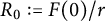 is called the basic reproduction number. It is easy to show that for either
$g_1$
 or
$g_2$
 , when the basic reproduction number
$R_0>1$
 , the coupled system will have a unique positive equilibrium. Obviously,
$(0,F(0))$
 is also an equilibrium, called a disease-free and behavioral-change-free equilibrium.
In what follows, we use
$f_1(x, y ):=\frac {\partial f(x, y)}{\partial x }$
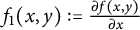 and
$ f_2(x, y ):=\frac {\partial f(x,y )}{\partial y}$
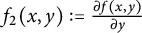 .
The linearization at a given equilibrium
$(\beta ^*,I^*)$
 of (2.1) is

Substituting
$I=e^{\lambda t}I_{\mathbf {o}}$
 ,
$\beta =e^{\lambda t}\beta _{\mathbf {o}}$
 leads to

Since
$f_{1}(x,y) )=F'(xy))y \leq 0$
 for
$y\ge 0$
 , we have that
$1-f_{1}(\beta ^*,g(I^*))e^{-\lambda \tau }\neq 0$
 for any
$\lambda \in \mathbb {C}$
 . So a characteristic equation of (2.3) is written as

We will explore the onset and global continuation of Hopf bifurcation from a positive equilibrium by using the
$S^1$
 -degree-based global Hopf bifurcation theory developed in [Reference Wu38]. Such a global Hopf bifurcation theorem has been developed for delay differential equations [Reference Erbe, Krawcewicz, Geba and Wu21] and for neutral equations with condensing fields [Reference Krawcewicz, Wu and Xia27]. Although system (2.3) can be considered as a neutral equation with initial conditions constrained in a sub-manifold of the phase space, the corresponding
$\mathcal {D}$
 -operator defined by

is not necessarily stable; thus, the
$ S^1$
 -degrees for condensing fields cannot be applied directly.
On the other hand, periodic solutions of (2.1) are defined for all
$t\in \mathbb {R}$
 . For these kinds of solutions, we can use the algebraic equation to solve
$\beta (t)$
 iteratively in terms of
$I(t-k\tau )$
 with
$k=1,2,\ldots $
 After substituting the iteration to the first equation of (2.1), we obtain a delay differential equation so that the right-hand side depends on
$I(t-k\tau )$
 with
$\tau \geq 0$
 , namely, a delay differential equation with infinite delay. To be more precise, we note

Define

with

According to the definition of
$f_{[k]}(x_{k}, y_k,\ldots , y_2, y_1)$
 ,
$ f_{[\infty ]}(\ldots , y_k,\ldots , y_2, y_1) $
 is well defined (in the sense of existence, not necessarily convergence) and satisfies the following property:
-
(C0) $f_{[\infty ]}(\ldots ,y_k,\ldots ,y_2,y_1)=f(f_{[\infty ]}(\ldots ,y_{k+1},y_k,\ldots ,y_2),g(y_1))$
.

We get

where
$I^t(s)=I(t+s)$
 for
$s\in \mathbb {R}$
 . Substituting (2.9) into the first equation of (2.1), we get

This motivates us to consider the global Hopf bifurcation theorem for functional differential equations with infinite delay formulated in [Reference Wu38], which we describe below.
2.2 Preliminary: Global Hopf bifurcation theory for FDEs with infinite delay
Let
$\mathbb {X}$
 denote the Banach space of bounded continuous mappings
$x:\mathbb {R}\to \mathbb {R}$
 equipped with the supremum norm. For
$x\in \mathbb {X}$
 and
$t\in \mathbb {R}$
 , we will use
$x^t$
 to denote an element in
$\mathbb {X}$
 defined by
$x^t(s)=x(t+s)$
 for
$s\in \mathbb {R}$
 .
Consider the following functional differential equation:

parameterized by two real numbers
$(a,p)\in \mathbb {R}\times \mathbb {R}_+$
 , where
$\mathcal {F}:=\mathbb {X}\times \mathbb {R}\times \mathbb {R}_+\to \mathbb {R}^n$
 is completely continuous. Identifying the subspace of
$\mathbb {X}$
 consisting of all constant mapping with
$\mathbb {R}^n$
 , we get a mapping
$\hat {\mathcal {F}}=\mathcal {F}|_{\mathbb {R}^n\times \mathbb {R}\times \mathbb {R}_{+}}:\mathbb {R}^n\times \mathbb {R}\times \mathbb {R}_{+}\to \mathbb {R}^n$
 . We assume
-
(A1). $\hat {\mathcal {F}}$
is twice continuously differentiable.

Denote by
$\hat {x}\in \mathbb {X}$
 the constant mapping with the value
$x_0\in \mathbb {R}$
 .
$(\hat {x}_0,a_0,p_0)$
 is a stationary solution of (2.11) if
$\hat {\mathcal {F}}(x_0,a_0,p_0)=0$
 .
-
(A2). At each stationary solution $(\hat {x}_0,a_0,p_0)$
, the derivative of
$\hat {\mathcal {F}}$
with respect to the first variable
$x$
, evaluated at
$(\hat {x}_0,a_0,p_0)$
is an isomorphism of
$\mathbb {R}^n$
.


Under (A1) and (A2), for each stationary solution
$(\hat {x}_0,a_0,p_0)$
 there exists
$\epsilon _0>0$
 and a continuously differential mapping
$y:B_{\epsilon _0}(a_0,p_0)\to \mathbb {R}^n$
 such that
$\hat {\mathcal {F}}(\hat {x}(a,p),a,p)=0$
 for
$(a,p)\in B_{\epsilon _0}(a_0,p_0)=(a_0-\epsilon _0,a_0+\epsilon _0)\times (p_0-\epsilon _0,p_0+\epsilon _0)$
 . We assume the following smoothness condition:
-
(A3). $\mathcal {F}(\varphi ,a,p)$
is differentiable with respect to
$\varphi $
, and the
$n\times n$
complex matrix function
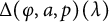
$\Delta (\varphi ,a,p)(\lambda )$
is continuous in
$(a,p,\lambda )\in B_{\varepsilon _0}(a_0,p_0)\times \mathbb {C}$
. Here, for each stationary solution
$(\hat {x}_0,a_0,p_0)$
, we have $$\begin{align*}\Delta(\hat{x}_0,a_0,p_0)(\lambda) = \lambda I_d -D\mathcal{F}(\hat{x}_0,a_0,p_0)(e^{\lambda \cdot}\mathrm{id}), \end{align*}$$
where $D\mathcal {F}(\hat {x}_0,a_0,p_0)$
is the complexification of the derivative of
$F(\varphi ,a,p)$
with respect to
$\varphi $
, evaluated at
$(\hat {x}_0,a_0,p_0)$
.








We call
$\Delta _{\hat {x}_0,a_0,p_0}(\lambda )$
 the characteristic matrix and the zeros of
$\det \Delta _{(\hat {x}_0,a_0,p_0)} (\lambda )=0$
 the characteristic values of
$(\hat {x}_0,a_0,p_0)$
 . A stationary solution
$(\hat {x}_0,a_0,p_0)$
 is called a center if it has purely imaginary characteristic values of the form
$i m \tfrac {2\pi }{p_0}$
 for some positive integer
$m$
 . A center
$(\hat {x}_0,a_0,p_0)$
 is said to be isolated if (i) it is the only center in some neighborhood of
$(\hat {x}_0,a_0,p_0)$
 ; (ii) it has only finitely many purely imaginary characteristic values of the form
$i m \tfrac {2\pi }{p_0}$
 ,
$m$
 an integer.
Assume
$(\hat {x}_0,a_0,p_0)$
 is an isolated center. Let
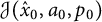
$\mathcal {J}(\hat {x}_0,a_0,p_0)$
 denote the set of all positive integers
$m$
 such that
$i m \tfrac {2\pi }{p_0}$
 is a characteristic value of
$(\hat {x}_0,a_0,p_0)$
 . We assume there exists
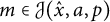
$m\in \mathcal {J}(\hat {x}_0,a_0,p_0)$
 such that
-
(A4) There exist $\varepsilon \in (0,\varepsilon _0)$
and
$\delta \in (0,\varepsilon _0)$
such that on
$[a_0-\delta ,a_0+\delta ]\times \Omega _{\varepsilon ,p_0}$
, we have
$\det \Delta (\hat {x}(a,p),a,p)(\mu +i m \tfrac {2\pi }{p})=0$
, if and only if
$a=a_0$
,
$\mu =0$
, and
$ p=p_0$
, where
$\Omega _{\varepsilon ,p_0} = \{ (\mu ,p);\ 0<\mu <\varepsilon ,\ p_0-\varepsilon < p < p_0+\varepsilon \}$
.







Define

Then (A4) implies
$\mathcal {H}_m^{\pm }(\hat {x}_0,a_0,p_0)\neq 0$
 on
$\Omega _{\varepsilon ,p_0}$
 . Consequently, the following integer:

is well defined, where
$\deg _B$
 is the Boruwer degree.
$\gamma _m(\hat {x}_0,a_0,p_0)$
 is called the mth crossing number of
$(\hat {x}_0,a_0,p_0)$
 . Further,
$\gamma \left (\hat {x}_0, a_0,p_0\right )\neq 0$
 implies the existence of a local Hopf bifurcation of periodic solutions with period
$p_0/m$
 . More precisely, if (A1)–(A3) are satisfied, and there exists an isolated center
$(\hat {x}_0,a_0,p_0)$
 and an integer
$m\in \mathcal {J}(\hat {x}_0,a_0,p_0)$
 such that (A4) holds and
$\gamma _m(\hat {x}_0,a_0,p_0)\neq 0$
 . Then there exists a sequence
$(a_k,p_k)\in \mathbb {R}\times \mathbb {R}_+$
 such that
-
(i) $ \lim _{k\to \infty } (a_k,p_k) = (a_0,p_0)$
; -
(ii) at each $(a,p)=(a_k,p_k)$
, (2.11) has a non-constant periodic solution
$x_k(t)$
with a period
$p_k/m$
;
$\lim _{k\to \infty }x_k(t)=\hat {x}_0$
, uniformly for
$t\in \mathbb {R}$
.






We can now state the global Hopf bifurcation theorem (Theorem 3.3 in [Reference Wu38]).
Theorem 2.3 Assume that
-
(GH1) All centers of (2.11) are isolated and (A4) holds for each center $(\hat {x}_0,a_0,p_0)$
and each
$m\in \mathcal {J}(\hat {x}_0,a_0,p_0)$
. -
(GH2) For each bounded set $W\subset \mathbb {X}\times \mathbb {R}\times \mathbb {R}_{+}$
, there exist a constant
$L>0$
such that
$|\mathcal {F}(\varphi ,a,p)-\mathcal {F}(\psi ,a,p))|\leq L\cdot \sup _{s\in \mathbb {R}}|\varphi (s)-\psi (s)|$
for
$(\varphi ,a,p), (\psi ,a,p)\in W$
.






Let

Assume that
$(\hat {x},a,p)$
 is an isolated center satisfying (A1)–(A4). Denote by
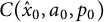
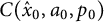
$ C(\hat {x}_0,a_0,p_0)$
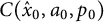 the connected component of
$(\hat {x}_0,a_0,p_0)$
 in
$\Sigma $
 , we have either
-
(i) $C(\hat {x}_0,a_0,p_0) $
is unbounded; or -
(ii) $C(\hat {x}_0,a_0,p_0)$
is bounded,
$C(\hat {x}_0,a_0,p_0)\cap N(\mathcal {F})$
is finite, and $$ \begin{align*}\sum_{(\hat{x},a,p) \in C(\hat{x}_0,a_0,p_0)\cap N(\mathcal{F})} \gamma\left(\hat{x},a,p \right) =0, \end{align*} $$
for all $m=1,2,\ldots $
where
$\gamma _m(\hat {x},a,p)$
is the
$m$
-th crossing number of
$(\hat {x},a,p)$
if
$m\in \mathcal {J}(\hat {x},a,p)$
or it is zero if otherwise.



2.3 Reformulation of the global Hopf bifurcation for delay-algebraic systems
We now reformulate this theorem in the setting of a delay-algebraic equation that is equivalent to (as far as solutions are defined for all
$t\in \mathbb {R}$
 ) the functional differential equation (2.10) with infinite delay.
The normalization of period by
$I(t)=x(\frac {2\pi }{T} t)$
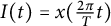 , where
$T>0$
 the period of periodic solutions
$I(t)$
 , gives
$I(t-k\tau )=x(\theta -k\frac {2\pi }{T} \tau )$
 with
$\theta =\frac {2\pi }{T} t$
 , and
$I^t=x(\theta +\frac {2\pi }{T}s)$
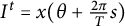 . Denote

where
$x^{\theta }=x(\theta +\frac {2\pi }{T} s)$
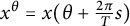 for
$s\in \mathbb {R}$
 .
Re-denoting
$\theta $
 as
$t$
 , system (2.10) is transformed into the following form:

where
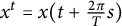
$x^{t}=x(t+\frac {2\pi }{T} s)$
 for
$s\in \mathbb {R}$
 .
The normalized system (2.12) has two bifurcation parameters,
$\tau $
 and
$T$
 .
$x(t)$
 is the periodic solution
$2\pi $
 -period for (2.12) if and only if
$I(t)$
 is a periodic solution
$T$
 -periodic for (2.10) (equivalently,
$(I(t),\beta (t))$
 is a periodic solution
$T$
 -periodic for (2.1)). Let
$ C_{2\pi } \times \mathbb {R}_+ \times \mathbb {R}_+$
 be the Fuller space, where
$C_{2\pi }$
 denotes the Banach space of
$2\pi $
 -periodic functions equipped with the sup-norm.
Then the corresponding
$\mathcal {F}(\cdot )$
 is as follows:

where
$x^t \in \mathbb {X}$
 . Identifying the subspace of
$\mathbb {X}$
 consisting of all constant functions with
$\mathbb {R}_{+}$
 , we obtain a restricted function
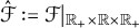
$\hat {\mathcal {F}}:=\mathcal {F}|_{\mathbb {R}_{+}\times \mathbb {R}\times \mathbb {R}_{+}}$
 .
Denote
$H_{[\infty ]}(x):= f_{[\infty ]}(x,x,x,\ldots )$
 . The property (C0) and Lemma 2.1 yield that
$H_{[\infty ]}(x)$
 is well defined, and it is the unique fixed point of the map
$u \mapsto f(u,g(x))$
 for
$u> 0$
 , that is,
$f \big (H_{[\infty ]}(x), g(x)\big ) = H_{[\infty ]}(x)$
 .
Additionally, we assume the following:
-
(S0) $H_{[\infty ]} (x)$
is
$C^2$
smooth as a function of
$x\ge 0$
.


Further, the following stronger condition ensures that the condition (S0) is satisfied (by the implicit function theorem).
-
(S0)′ $f_1(H_{[\infty ]}(x),g(x))\neq 1$
for all
$x\ge 0$
.


Since
$p\tau (H_{[\infty ]}(x)g(x)-rx)$
 is twice continuously differentiable, we have the following result.
Lemma 2.4
$\hat {\mathcal {F}}$
 is twice continuously differentiable, that is, condition (A1) is satisfied.
The stationary points
$\hat {x}$
 of (2.10) (or (2.12)) can be obtained by solving

Then the set of stationary solutions of system (2.12) is

Obviously, as long as
$(\hat {x},\tau ,T)\in \mathcal {N}(\mathcal {F})$
 , it necessarily follows that
$H_{[\infty ]}(\hat {x})=F(r\hat {x})$
 .
We define

For any stationary solution
$(\hat {x},\tau ,T)\in \mathcal {N}(\mathcal {F})$
 , the characteristic function is

Let

Define
$\partial _{k} f_{[\infty ]}(\ldots ,y_3,y_2,y_1):=\frac {\partial f_{[\infty ]}(\ldots ,y_k,\ldots ,y_2,y_1)}{\partial y_k}$
 , where
$y_k$
 is the
$k$
 -th argument from the right (with
$y_1$
 the outermost). Then from (C0) it follows that

We get

We impose the following assumption to ensure that
$\sum _{j=1}^\infty \partial _{j}f_{[\infty ]}(\ldots ,\hat {x},\hat {x})e^{-j \frac {2\pi }{T}\lambda \tau }$
 is well defined.
-
(S1) For any $(\hat {x},\tau ,T)\in \mathcal {N}(\mathcal {F})$
,
$1-e^{- \frac {2\pi }{T}\lambda \tau }f_1(H_{[\infty ]}(\hat {x}),g(\hat {x}))\neq 0$
holds for all
$\lambda \in \mathbb {C}$
.



We have the following result about the characteristic function
$ \det \Delta _{(\hat {x},\tau ,T)}(\lambda )$
 .
Lemma 2.5 If condition (S1) holds, then

Moreover, we have

To ensure that there is no root of
$\det \Delta _{(\hat {x},\tau ,T)}(\lambda )=0$
 entering the right (left) half of the complex plane from the left (right) half through infinities, we give the following assumption.
-
(S1a) For any $(\hat {x},\tau ,T)\in \mathcal {N}(\mathcal {F})$
,
$\left |f_1(H_{[\infty ]}(\hat {x}),g(\hat {x}))\right |<1$
holds.


Clearly, the assumption (S1a) guarantees that (S1) holds for all
$\operatorname {Re}\lambda \ge 0$
 .
From formula (2.2), we find that the equilibrium component
$I^*$
 of (2.1) is identical to the stationary point of (2.10), with
$H_{[\infty ]}(I^*)=\beta ^*$
 . And by comparing the characteristic equation
$\Delta _{\mathrm {S}}(E^*,\tau )(\lambda )$
 defined in (2.5) and
$ \det \Delta _{(\hat {x},\tau ,T)}(\lambda )$
 in (2.17), we obtain the following result.
Lemma 2.6 If
$(\hat {x},\tau ,T)\in \mathcal {N}(\mathcal {F})$
 , then
$\hat {E}:=(\hat {x},H_{[\infty ]}(\hat {x}))$
 is an equilibrium of the delay-algebraic system (2.1). Further,

Consequently, we have the following lemma.
Lemma 2.7 If the following assumption holds:
-
(S2) For any $(\hat {x},\tau ,T)\in \mathcal {N}(\mathcal {F})$
,
$\Delta _{\mathrm {S}}(\hat {E}(\tau ,T),\tau )(0)\neq 0$
(i.e.,
$\det \Delta _{(\hat {x},\tau ,T)}(0)\neq 0$
),



then condition (A2) is satisfied.
In addition, it can be easily checked from (2.13) that the smoothness condition (A3) is also satisfied.
Denote the set of centers of (2.12) by

where
$\mathcal {J}(\hat {x},\tau ,T)$
 is the set of all positive integers
$m$
 such that
$\Delta _{\mathrm {S}}(\hat {E},\tau )(im\frac {2\pi }{T})=0$
 . (Equivalently,
$im$
 is a characteristic value of
$(\hat {x},\tau ,T)$
 .)
For a given isolated center
$(\hat {x}_0, \tau _0, T_0)\in \mathcal {N}_c(\mathcal {F})$
 , the corresponding
$\hat {E}_0:=(\hat {x}_0,H_{[\infty ]}(\hat {x}_0))$
 is an equilibrium of (2.1) from Lemma 2.6, we assume that there exists
$m\in \mathcal {J}(\hat {x}_0, \tau _0, T_0)$
 such that
-
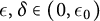
(S3) There exist $\epsilon ,\delta \in (0,\epsilon _0)$
such that
$[\tau _0-\delta ,\tau _0+\delta ]\times \partial \Omega _{\epsilon , T_0}$
with
$\partial \Omega _{\epsilon , T_0}=\{(\mu ,T):0<\mu <\epsilon , T_0-\epsilon <T< T_0+\epsilon \}$
,
$\Delta _{\mathrm {S}}(\hat {E}(\tau ,T),\tau )\left (\frac {2\pi }{T}\mu +im\frac {2\pi }{T}\right )=0$
(i.e.,
$\det \Delta _{(\hat {x}(\tau ,T),\tau ,T)}(\mu +im)=0$
) if and only if
$\mu =0$
,
$T=T_0$
, and
$\tau =\tau _0$
.






In what follows, we denote
$\hat {E}(\tau _0\pm \delta ,T):=\left (\hat {x}(\tau _0\pm \delta ,T),H_{[\infty ]}\left (\hat {x}(\tau _0\pm \delta ,T)\right )\right )$
 , and let

Hence, we obtain the following result.
Lemma 2.8 Supposed that (S3) holds (i.e., (A4) is satisfied), implying no zero of
$\Delta _{\mathrm {S}}(\hat {E}_0,\tau )\left (\frac {2\pi }{T}\mu +im\frac {2\pi }{T}\right )=0$
 (i.e.,
$\det \Delta _{(\hat {x}_0,\tau _0,T_0)}(\mu +im)= 0$
 ) in
$\partial \Omega _{\epsilon ,T_0}$
 . Then the mth crossing number of
$(\hat {x}_0,\tau _0,T_0)$
 :

is well defined.
Lemma 2.9 For every bounded set
$W\subset \mathbb {X}\times \mathbb {R}\times \mathbb {R}_{+}$
 , there exists
$L_{\mathcal {F}}>0$
 such that

where

That is, (GH2) is satisfied.
Proof By the triangle inequality, we have

Since
$f,g$
 is
$\mathbb {C}^2$
 -smooth, by the mean value theorem, we can get the constant
$L_{\mathcal {F}}<\infty $
 directly.
We can now state the following local and global Hopf bifurcation theorems for delay-algebraic system (2.1).
Theorem 2.10 For delay-algebraic system (2.1), suppose that (S0), (S1), (S1a), and (S2) are satisfied and there exists an isolated center
$(\hat {x}_0,\tau _0,T_0)$
 and an integer
$m\in \mathcal {J}(\hat {x}_0,\tau _0,T_0)$
 such that (S3) holds and
$\gamma _m(\hat {x}_0,\tau _0,T_0)\neq 0$
 . Then there exists a sequence
$(\tau _k,T_k)\in \mathbb {R}_+\times \mathbb {R}_+$
 such that
-
(i) $\lim _{k\to \infty }(\tau _k,T_k)=(\tau _0,T_0)$
; -
(ii) at each $(\tau _k,T_k)$
, system (2.1) has nontrivial periodic solution
$(I_k(t),\beta _k(t))$
with a period
$T_k/m$
: $$ \begin{align*}\lim_{k\to\infty}(I_k(t),\beta_k(t))=(\hat{x}_0,H_{[\infty]}(\hat{x}_0)),\,\, \text{uniformly for}\,\, t\in\mathbb{R}.\end{align*} $$





Theorem 2.11 (Global Hopf bifurcation theorem)
For delay-algebraic system (2.1), suppose that
-
(AH1) All $(\hat {x},\tau ,T)\in \mathcal {N}_c(\mathcal {F})$
are isolated and condition (S3) holds for each
$(\hat {x},\tau ,T)\in \mathcal {N}_c(\mathcal {F})$
and every
$m\in \mathcal {J}\left (\hat {x},\tau ,T\right )$
.



Assume that
$(\hat {x}_0,\tau _0,T_0)$
 is an isolated center satisfying conditions (S0), (S1), (S1a), and (S2). Denote by the connected component
$ C(\hat {x}_0,\tau _0,T_0)$
 of
$(\hat {x}_0,\tau _0,T_0)$
 in
$\Sigma (\mathcal {F})$
 , we have either
-
(i) $C(\hat {x}_0,\tau _0,T_0) $
is unbounded; or -
(ii) $C(\hat {x}_0,\tau _0,T_0) $
is bounded,
$C(\hat {x}_0,\tau _0,T_0)\cap \mathcal {N}(\mathcal {F})$
is finite, and $$ \begin{align*}\sum_{(\hat{x},\tau,T) \in C(\hat{x}_0,\tau_0,T_0)\cap \mathcal{N}(\mathcal{F})} \gamma\left(\hat{x},\tau,T\right) =0, \end{align*} $$




for all
$m=1,2,\ldots $
 , where
$\gamma _m(\hat {x},\tau ,T)$
 is the
$m$
 th crossing number of
$(\hat {x},\tau ,T)$
 if
$m\in \mathcal {J}(\hat {x},\tau ,T)$
 , or it is zero if otherwise.
To examine the boundedness of global Hopf branches of delay-algebraic system (2.1), we need to explore the boundedness of the projection of
$C(\hat {x}_0,\tau _0,T_0) $
 onto the parameter (
$\tau $
 ) space, the
$\mathbb {X}$
 -space, and the
$T$
 -space, respectively. If the projections of
$C(\hat {x}_0,\tau _0,T_0) $
 onto the parameter (
$\tau $
 ) space, the
$\mathbb {X}$
 -space, and
$T$
 -space are all bounded, then (ii) of Theorem 2.11 must hold, implying that the sum of crossing numbers along the bounded branch must be zero. Conversely, if this sum along any such branch cannot be zero, then one of the projections of a given connected component must be maximal.
3 Equivalent cyclic ODE systems for periodic solutions with pre-scribed delays
3.1 Preliminary
We describe some preliminary results as preparation and introduce a few notions:

with
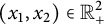
$(x_1,\ldots ,x_{n})\in \mathbb {R}^n_{+}$
 . Since
$G(u;x_n,x_{n-1} \ldots ,x_1)$
 is monotonic with respect to
$u\geq 0$
 , increasing if
$n$
 is even and decreasing if
$n$
 is odd (due to
$f_1(x,y) < 0$
 ), and

then

must have a positive fixed point in
$(0,\beta _c)$
 . Assume that
-
(C1). The positive fixed point of (3.2) in $(0,\beta _c)$
is unique, denoted by (3.3) $$ \begin{align} u^*:=H(x_{1},x_{2},\ldots,x_{n}). \end{align} $$


$H(\cdot )$
 can be regarded as a
$n$
 variable functions with
$(x_{1},x_{2},\ldots ,x_{n})\in \mathbb {R}^n_+$
 . When
$n$
 is odd, (C1) holds naturally.
For brevity, denote

and
$u_n:=u^*$
 . Then
$u_0=G(u;x_1,\ldots ,x_n)$
 and
$u_{j-1}=f(u_{j},x_{j})$
 for
$j=1,\ldots ,n$
 .
To ensure existence of
$\partial u^*/\partial x_j$
 , we assume that
-
(C2). $ 1-\prod _{k=1}^{n} f_1(u_k,x_k)\neq 0. $

When
$n$
 is odd, (C2) holds naturally.
Lemma 3.1 (Monotonicity of the function
$H$
)

If (C2) holds, then

where
$H_j(x_1,x_2,\ldots ,x_n):=\frac {\partial H(x_1,x_2,\ldots ,x_n)}{\partial x_{j}}$
 .
Proof Taking the derivative of (3.2) with respective to
$x_j$
 on both sides, we obtain

with


Hence, we obtain

Since
$f_1(x,y)=F'(xy)y<0$
 ,
$f_2(x,y)=F'(xy)x<0$
 , we obtain

For the cases
$n=2,3$
 , we have
Corollary 3.2
-
(i) $ \operatorname {Sign}(H_1(x_1,x_2)) = -\operatorname {Sign}(H_2(x_1,x_2)) $
for
$(x_1,x_2)\in \mathbb {R}_+^2$
; -
(ii) $ \operatorname {Sign}(H_1(x_1,x_2,x_3)) = -\operatorname {Sign}(H_2(x_1,x_2,x_3))=\operatorname {Sign}(H_3(x_1,x_2,x_3))<0 $
for
$(x_1,x_2,x_3)\in \mathbb {R}_+^3$
.



Lemma 3.3 Let
$\{y_k\}_{k\in \mathbb {Z}}$
 be an
$n$
 -cyclic sequence, that is,
$y_{k+n} = y_k$
 for all
$k \in \mathbb {Z}$
 ,
$y_k \in \mathbb {R}_+$
 . Then

In the particular case, if
$n=1$
 , we have
$H_{[\infty ]}(y_1)=H(g(y_1),g(y_1),\ldots ,g(y_1))$
 .
Proof From property (C0) of
$f_{[\infty ]}(\ldots ,y_n,y_{n-1},\ldots ,y_1)$
 , it follows that

Since
$(y_k)_{k\in \mathbb {Z}}$
 is cyclical, we have

which holds if and only if
$f_{[\infty ]}(\ldots ,y_{n+1},y_n,y_{n-1},\ldots ,y_1)$
 is the unique positive fixed point of

Hence,
$ f_{[\infty ]}(\ldots ,y_n,y_{n-1},\ldots ,y_1)=H(g(y_1),\dots ,g(y_n)), $
 where the function
$H(\cdot )$
 of
$ n $
 -variables is given as the positive solution of (3.2).
Theorem 3.4 For a nontrivial periodic solution of period
$ n\tau $
 for system (2.10), denoted by
$\tilde {I}(t)$
 , we have

where
$H(\cdot )$
 is given as a positive solution of (3.2). Furthermore, the existence of such an
$ n\tau $
 -periodic solution for system (2.10) implies the following n-dimensional autonomous ODE system:

has a nontrivial
$n\tau $
 -periodic solution
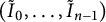
$(\tilde {I}_0,\ldots ,\tilde {I}_{n-1})$
 , where
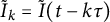
$\tilde {I}_k=\tilde {I}(t-k\tau )$
 ,
$k=0, 1,\ldots n-1$
 . In particular, if
$\tilde {I}(t)$
 is a
$\tau $
 -periodic solution of (2.10), then is also a
$\tau $
 - periodic solution of the following ODE:

Proof Suppose
$\tilde {I}(t)$
 is an
$n\tau $
 -periodic solution of (2.10) and define
$ \tilde {I}_j(t):=\tilde {I}(t-j\tau )$
 ,
$j=0,\ldots ,n-1$
 , and
$ \tilde {I}_j(t-\tau )=\tilde {I}_{j+1}(t),\,\,\tilde {I}_0(t)=\tilde {I}(t),\,\, \tilde {I}_k(t-n\tau )=\tilde {I}_{k+n}(t)=\tilde {I}_k(t). $
 Then

Because
$\tilde {I}(t)$
 is
$n\tau $
 -periodic, the sequence
$\{\tilde {I}_k(t)\}_{k\ge 1}$
 is
$n$
 -cyclic in
$k$
 .
By Lemma 3.3, we have

Then we get the following
$n$
 -dimensional autonomous ODE system:

which means that
$(\tilde {I}_0,\tilde {I}_1,\ldots ,\tilde {I}_{n-1})$
 is a
$n\tau $
 -periodic solution of system (3.5).
Remark 3.5 The established approach to understand the global continuation of a local branch of Hopf periodic solutions involves obtaining bounds on the amplitudes of periodic solutions and excluding the existence of periodic solutions with periods of the form
$n\tau $
 , where
$n$
 is a positive integer. According to Theorem 3.4, in order to exclude
$n\tau $
 -periodic solutions of (2.10), it is sufficient to exclude nontrivial periodic solutions of the corresponding ODE system (3.5).
3.2 Some properties of the equivalent ODE system
We start with listing a few propositions.
Proposition 3.6 The set
$ \mathcal {D}_n := \{ (I_0,I_1,I_2,\ldots I_{n-1})\in \mathbb {R}_+^n |I_0 = I_1 = I_2=\cdots =I_{n-1} \} $
 is invariant with respect to ODE (3.5).
Proposition 3.7 (Cyclic permutation operator on
$\mathbb {R}^n$
)

Let

be an arbitrary solution of system (3.5) with the initial condition
$ \gamma (0) $
 . Let
$ \boldsymbol {x} = (x_0, x_1, \dots , x_{n-1})^\top \in \mathbb {R}^n $
 and define the cyclic shift operator
$ \sigma \colon \mathcal {L}_n\to \mathcal {L}_n $
 by
$ \sigma (\boldsymbol {x}) := (x_1, x_2, \dots , x_{n-1}, x_0)^\top , $
 which is bijection with
$ \sigma ^n = \mathrm {id} $
 , the identity map. Then, for each
$ k = 1, 2\ldots ,n$
 , the permuted
$ \sigma ^k(\gamma (t)) $
 , is also a solution of system (3.5) with initial condition
$ \sigma (\gamma (0))$
 . Moreover,
$\gamma (t)$
 ,
$\sigma (\gamma (t))$
 ,
$\sigma ^2(\gamma (t))$
 ,…,
$\sigma ^n(\gamma (t))$
 are isomorphic in
$ \mathcal {L}_n $
 .
Proposition 3.8 (Isomorphism)
$\mathfrak {S}_n$
 is the symmetric group on the set
$\{0, 1, \dots , n-1\}$
 . Let
$ \pi \in \mathfrak {S}_n $
 and define the corresponding relabeled system by:

which is topologically conjugate to system (3.5) via the coordinate relabeling:

Then
$ (\tilde {I}_0, \dots , \tilde {I}_{n-1}) = \Phi _\pi (I_0, \dots , I_{n-1}) $
 . That is, if
$ \gamma (t) = (I_0(t), \dots , I_{n-1}(t)) $
 is a solution of the original system, then
$ \Phi _\pi (\gamma (t)) $
 is a solution of the permuted system (3.9). In addition, trajectories
$ \gamma (t)$
 and
$ \Phi _\pi (\gamma (t)) $
 are isomorphic in
$ \mathcal {L}_n $
 .
These results are natural consequence of the equivalence of the ODE vector field with respect to the cyclic group (see [Reference Balanov, Krawcewicz, Rachinskii, Wu and Yu3, Reference Golubitsky, Stewart and Schaeffer23]). For the sake of completeness, we provide some direct proof for Propositions 3.6–3.8, which are given in the Appendix.
Specifically, system (3.5) for
$n = 2$
 reduces to the following planar system:

By Proposition 3.6 and using the uniqueness of solutions, we obtain the following result.
Lemma 3.9 For system (3.10), the diagonal region
$\mathcal {D}_2:=\{ (I_0, I_1) \in \mathbb {R}_{+}^2 \mid I_0 = I_1 \}$
 and the regions
$\Omega _+ := \{ (I_0, I_1) \in \mathbb {R}_ + ^2 : I_0> I_1 \}$
 ,
$\Omega _- := \{ (I_0, I_1) \in \mathbb {R}_+^2 : I_0 < I_1 \} $
 are invariant manifolds with
$ \mathbb {R}_+^2=\Omega _+\cup \Omega _- \cup \mathcal {D}_2 $
 . Consequently, any possible limit cycle must lie entirely within either
$ \Omega _+ $
 or
$\Omega _-$
 .
To exclude periodic solutions of system (3.10), we need an additional assumption:
-
(H1a) $g'(x)>0$
for
$x\ge 0$
.


To apply Lemma 3.2-(i), we need the following assumption on
$g$
 .
-
(H1b) $\operatorname {Sign}(H_2(y_1,y_2))(g'(x)x-g(x)) \ge 0$
for
$y_1,y_2,x\ge 0$
.


Theorem 3.10 Suppose that (H1a) and (H1b) are satisfied. Then system (3.10) admits no non-constant periodic solution in any region of the positive quadrant
$ \mathbb {R}_+^2 $
 .
Proof By Proposition 3.7 and Lemma 3.9, we only need to exclude the existence of non-constant periodic solution within one of
$\Omega _+$
 or
$\Omega _-$
 . We state the proof for
$\Omega _+$
 .
Define the scalar function:

We compute the derivative of
$V(t):=V(I_0(t), I_1(t))$
 along trajectories of the system as follows:

Therefore, if
$H_2<0, \text { then } H_1>0$
 by Corollary 3.2 (i), and if
$g'(x)x-g(x)\le 0,$
 we have

for all
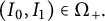
$ (I_0,I_1)\in \Omega _+.$
 Consequently,
$ \frac {dV(t)}{dt}<0.$
 Similarly, if
$ H_2>0$
 and
$ g'(x)x-g(x) \ge 0,$
 using the same argument we obtain
$ \frac {dV(t)}{dt}>0$
 . Thus,
$ V(I_0(t),\, I_1(t)) $
 strictly monotonic on
$\Omega _+$
 , given that (H1a) and (H1b) hold. Now suppose, for contradiction, that there exists a nontrivial periodic solution
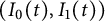
$ (I_0(t), I_1(t)) $
 with period
$ T> 0 $
 . Then
$ V(0) = V(T) $
 must hold. But this contradicts with the strict monotonicity of
$ V(t) $
 . Hence, no limit cycle exists in any region of the positive quadrant
$ \mathbb {R}_+^2$
 .
Lemma 3.11 Suppose that (H1a) and (H1b) are satisfied. Then system (2.10) (or (2.1)) has no
$2\tau $
 periodic solutions, and consequently, system (2.10) has no periodic solutions with period
$2\tau /m$
 for any positive integer
$m$
 .
We also note the following Lemma.
Lemma 3.12 The period of potential periodic solutions of (2.10) cannot be
$\tau $
 ; consequently, system (2.10) does not have
$\tau /m$
 periodic solutions for any integer
$m$
 .
The global dynamics of ODE system (3.5) with high dimension (
$n \geq 3$
 ) is more delicate than the two-dimensional case and poses substantial analytical challenges. Li–Muldowney’s technique [Reference Li and Muldowney28] has been widely used to rule out nontrivial solutions, which is critical for us to use the global Hopf bifurcation theory. To use this approach, we first note that the Jacobian matrix associated with a general solution of (3.5) is
$J_n := \big ( (J_n)_{k\ell } \big )_{0\le k,\ell \le n-1}$
 with entries

where
$m$
 is the position of
$I_\ell $
 in the ordered list
$(I_{k+1\bmod n}, I_{k+2\bmod n}, \ldots , I_{k+n-1\bmod n}, I_k)$
 and

From the definition of the function
$H(x_1,x_2,\ldots ,x_0)$
 , we obtain

Therefore,

It follows the following lemma.
Lemma 3.13
$f(\beta _k,I_k)=\beta _{k+n-1 \bmod n}$
 ,
$k=0,1,\ldots ,n-1$
 .
Denote by
$J_n^{[2]}$
 the second addictive compound matrix of
$J_n$
 and by
$\mu (\cdot )$
 the Lozinskii measure [Reference Coppel13] corresponding to an absolute norm
$|\cdot |$
 . An application of Corollary 3.5 in [Reference Li and Muldowney28] yields the following lemma.
Lemma 3.14 Suppose that either
$\mu (J_n^{[2]})<0$
 or
$\mu (-J_n^{[2]})<0$
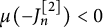 holds for all
$(I_0,I_1,\ldots ,I_{n-1})\in \Omega ^n\subseteq \mathbb {R}_{+}^n$
 , then system (3.5) has no non-constant periodic solution entirely contained in the region
$ \Omega ^n$
 .
4 Case study: The Zhang–Scarabel–Murty–Wu outbreak model
We now pull everything developed far together to consider Zhang–Scarabel–Murty–Wu outbreak model

where
$\beta (t)$
 is the incidence rate,
$r$
 is the removal rate (from
$I$
 class) that includes death and recovery. The incidence is
$B(t):=\beta (t)I(t)$
 and the reproduction number is
$R_0=\beta _c/r$
 . Here,
$ F(\xi ) = \frac {\beta _c}{1 + \kappa \xi } $
 and
$g(x)=x$
 satisfy (H1) and (H2).
Solving
$f(y,g(x))=y$
 for
$y$
 yields

Thus, (S0) is satisfied.
4.1 The local bifurcation of the Zhang–Scarabel–Murty–Wu outbreak model
The endemic equilibrium of system (4.1) is

It is easy to verify that
$ H_{[\infty ]}(I^*)=\beta ^*=r$
 .
It was shown in [Reference Zhang, Scarabel, Murty and Wu39] that
$E_0:=(I_0,\beta _0)=(0,\beta _c)$
 is stable if
$R_0<1$
 ; and if
$R_0>1$
 , then
$E_0$
 is unstable and system (4.1) has a unique inner equilibrium
$E^*=(I^*,\beta ^*)$
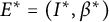 given by (4.3). Hence,

Obviously,
$\left ( 1 + \frac {R_0 - 1}{R_0} e^{-\lambda \tau } \right )\neq 1$
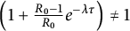 for any
$\lambda \in \mathbb {C}$
 . The characteristic equation for the linearization of system (4.1) at the endemic equilibrium
$E^*$
 is

We note that
$\Delta _{\mathrm {S}}(E^*,\tau )(0)\neq 0$
 if
$R_0>1$
 , hence, (S2) is satisfied.
In [Reference Zhang, Scarabel, Murty and Wu39], the issue of local Hopf bifurcation was considered when
$R_0>1$
 . It was shown that there exists a critical
$\tau ^*$
 such that: when
$\tau \in [0,\tau ^*)$
 , all real parts of the eigenvalue are negative, and
$E^*$
 is locally asymptotically stable. However, if
$\tau $
 passes through the critical value:
$\tau _0$
 and other
$\tau _k, k\ge 1$
 , there will be local Hopf bifurcations of periodic solutions. More precisely, at each
$\tau =\tau _k$
 , there appears a pair of purely imaginary eigenvalues
$\pm i \omega ^*$
 . When
$\tau \in (\tau _k,\tau _{k+1}]$
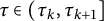 , there are
$k+1$
 pairs of eigenvalues with positive real part, so
$E^*$
 is unstable for
$\tau>\tau ^*$
 ; system (4.1) undergoes a Hopf bifurcation of periodic solutions at
$E^*$
 when
$\tau $
 passes through
$\tau _k$
 for each
$k=0,1,2,\ldots $
 , where


and then

satisfying
$\Delta _{\mathrm {S}}(E^*,\tau _k)(\omega ^* i)=0$
 ,

and

Since

condition (S1) is satisfied. Moreover, because
$(R_0-1)/R_0\in (0,1)$
 , condition (S1a) also holds. Then, by Lemma 2.5, we have

for any
$\lambda \in \mathbb {C}$
 , which also verifies conditions in Lemma 2.6. Based on the local Hopf bifurcation result of system (4.1), we obtain that
$T^*=\frac {2\pi }{\omega ^*}$
 ,
$m=1\in \mathcal {J}(I^*,\tau _k,T^*)$
 and
$\det \Delta _{(I^*,\tau _k,T^*)}\left (i\right )=0$
 , which means that
$\mathcal {N}_c(\mathcal {F})=\{(I^*,\tau _k,T^*),k=0,1,2\ldots \}$
 and any
$(I^*,\tau _k,T^*)$
 is isolated.
For any fixed
$k$
 , there exist
$\delta>0$
 and a smooth curve
$\lambda :(\tau _k-\delta ,\tau _k+\delta )\to \mathbb {C}$
 such that
$\Delta _{\mathrm {S}}(E^*,\tau )(\lambda (\tau ))=0$
 ,
$ |\lambda (\tau ) - i\omega ^*| < \epsilon $
 for all
$ \tau \in (\tau _k - \delta , \tau _k+ \delta )$
 , and

Let
$\Omega _{\epsilon ,T^*} =(0,\epsilon )\times (T^*-\epsilon ,T^*+\epsilon )$
 . If
$|\tau - \tau _k| \leq \delta $
 and
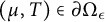
$(\mu , T) \in \partial \Omega _\epsilon $
 such that
$\Delta _{\mathrm {S}}(E^*,\tau )(\lambda (\tau )) (\frac {2\pi }{T}\mu + \frac {2\pi }{T}i) = 0$
 , then
$\mu = 0$
 ,
$T = T^*$
 (i.e.,
$\frac {2\pi }{T}=\omega ^*$
 ), and
$\tau = \tau _k$
 . Hence, condition (S3) is satisfied for any
$k=0,1,2,\ldots $
 Furthermore, it follows from Lemma 2.8, that the first crossing number of
$(I^*,\tau _k,T^*)$
 is

In summary, for system (4.1), given that
$R_0>1$
 , then any
$(I^*,\tau _k,T^*)\in \mathcal {N}_c(\mathcal {F})=\{(I^*,\tau _k,T^*),k=0,1,2,\ldots \}$
 is isolated and condition (S3) holds for any
$(I^*,\tau _k,T^*)$
 with
$m=1$
 . In addition, the isolated center
$(I^*,\tau ^*,T^*)$
 satisfies (S0), (S1), (S1a), and (S2). Denote by
$C(I^*, \tau _k, T^*)$
 the connected component through
$(I^*, \tau _k, T^*)$
 in
$\Sigma (\mathcal {F})$
 , for
$k = 0, 1, 2, \dots $
 Then, we have

This allows us to apply Theorem 2.11 to obtain the following result.
Theorem 4.1 Given that
$R_0>1$
 .
$C(I^*, \tau _k, T^*)$
 is unbounded for any
$k = 0, 1, 2, \dots $

From (4.6), we know
$\frac {\pi }{2}<\omega ^*\tau ^*<\pi ,\,\ 2\pi <\omega ^*\tau _k<(2k+1)\pi ,\,k\geq 1.$
 Therefore,
$2<\frac {T^*}{\tau ^*}<4,\,\,\,\frac {1}{k+1}<\frac {T^*}{\tau _k}<1,\,\, k\geq 1, $
 and
$\tau _k>T^*,\,\,k=1,2,\ldots $
 Then for
$\tau>\tau _k$
 , there exists an integer
$n$
 such that
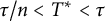
$\tau /n<T^*<\tau $
 . Thus, we obtain the following remark.
Remark 4.2 Periodic solutions of (4.1) on the first Hopf branch based at
$\tau ^*$
 have period
$T^*$
 bounded between
$2\tau ^*$
 and
$4\tau ^*$
 . Moreover, if
$R_0>2$
 , period
$T^*$
 is bounded between
$2\tau ^*$
 and
$3\tau ^*$
 (see Figure 1-(a,b)), and thus periodic solutions on the first Hopf branch are slowly varying. Meanwhile, periodic solutions on other Hopf branches
$\tau _k$
 with
$k>1$
 have periods smaller than
$\tau _k$
 and thus are fast oscillating. In particular, if
$ R_0> 2 $
 (and hence,
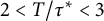
$ 2 < T/\tau ^* < 3$
 ), and if system (4.1) has no
$2\tau $
 and
$3\tau $
 nontrivial periodic solution, then the period
$T$
 of a periodic solution on the connected component
$C(I^*,\tau ^*,T^*)$
 satisfies
$T\in (2\tau ,3\tau )$
 . These periodic solutions bifurcating from the first branch, slowly oscillating periodic solutions, resemble those slowly oscillating periodic solutions, intensively studied [Reference Diekmann, van Gils, Verduyn Lunel and Walther14, Reference Guo and Wu24], for delay differential equations.
An illustration of the difficulty in obtaining lower and upper bounds of periodic solutions of a delay-algebraic system when varying the delay. (a) The
$R_0$
 –
$T/\tau ^*$
 plane with
$r=0.5$
 . (b) Ratio of period to delay for periodic solutions of (4.1) while varying
$\tau $
 , with
$\kappa =0.05$
 and
$\beta _c=0.7143$
 , for
$R_0=2$
 (
$\!\! \tau ^*=10.1571$
 , yellow),
$R_0=3$
 (
$\!\! \tau ^*=10.8025$
 , purple),
$R_0=1.0753$
 (
$\tau ^*=35.2005$
 , blue), and
$R_0=1.3889$
 (
$\!\! \tau ^*=12.3638$
 , orange); These numerical simulations demonstrate that a relatively large
$R_0$
 , specifically
$R_0>2$
 , ensures that the ratio
$T/\tau $
 is below
$3$
 . The solution curve of
$ I(t) $
 when
$ \tau ^*=12.3638$
 : upper panel shows the long-term periodic pattern, bottom panel shows the periodic wave comes as a spike with large amplitude in short time (within 90 days). Here, the delay
$ \tau $
 and the period T are measured in days, consistent with the parameterization adopted in [Reference Zhang, Scarabel, Murty and Wu39].

Figure 1 Long description
Panel a is a line graph titled R sub 0 minus T all over tau super asterisk for r = 0.5. The x-axis is R sub 0 ranging from 0 to 60, and the y-axis is T all over tau super asterisk ranging from 2 to 4. A red curve shows a steep exponential decay from R sub 0 = 1 to R sub 0 = 10, then levels off asymptotically toward 2.1. An inset graph shows a close-up for R sub 0 between 1 and 2.
Panel b is a scatter plot with tau on the x-axis (0 to 130) and T sub min all over tau on the y-axis (0 to 14). It contains four colored data series. A purple line remains flat near y = 2.5. A yellow line remains flat near y = 3. An orange line increases slightly then plateaus near y = 4.5. A blue line shows a steep linear increase starting from tau = 35, reaching y = 12.
Panel c consists of two vertically stacked time-series plots for I(t). The top plot shows a long-term periodic pattern with sharp blue spikes of equal height (1.6 times 10 super 6) occurring at regular intervals across a time t from 0 to 10,000. The bottom plot is a zoom-in on the interval 0 to 90, showing a single blue spike that begins to rise sharply after t = 70, reaching 3.5 times 10 super 5 by t = 90.
So our next goal is to exclude the existence of
$2\tau -$
 and
$3\tau -$
 nontrivial periodic solutions of system (4.1). Based on Theorem 3.4, it is sufficient to rule out the existence of
$2\tau -$
 and
$3\tau -$
 nontrivial periodic solutions of the corresponding ODE system (3.5) with
$n=2,3$
 .
4.2 Exclusion of nontrivial periodic solution of the equivalent ODE system
Since
$g(x)=x$
 satisfies (H1a) and (H1b), from Theorem 3.10 and Lemma 3.11, it follows the following lemma.
Lemma 4.3 System (4.1) has no
$2\tau -$
 nontrivial periodic solution.
Next, we discuss the case
$n=3$
 . The corresponding function
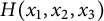
$H(x_1,x_2,x_3)$
 can then be explicitly computed as follows:

which is positive in its domain. Moreover,
$H(x_1,x_2,\infty )=\frac {\kappa \beta _c}{\kappa (\kappa \beta _c x_1+1)}<\beta _c$
 ,
$H(0,0,0)=\beta _c$
 , and

which is strictly decreasing in
$x$
 with
$\lim _{x\to \infty }H_{[\infty ]}(x)=0$
 and
$H(I^*,I^*,I^*)=H_{[\infty ]}(I^*)=r$
 .
Then, system (A.1) is specified as follows:

To rule out existence of periodic solutions of system (4.12), we first obtain the Jacobian matrix associated with a general solution of (4.12) as follows:

where
$\beta _0=H(I_1,I_2,I_0)$
 ,
$\beta _1=H(I_2,I_0,I_1)$
 , and
$\beta _2=H(I_0,I_1,I_2)$
 . According to (3.4) and Lemma 3.13, we have

where

and

Denote by
$\mu _2(\cdot )$
 the Lozinskii measure [Reference Coppel13] with respect to the Euclidean norm
$\|\cdot \|_2$
 . Let
$S_0 := \alpha \, J_3^{[2]}$
 and
$S_1 := \frac {S_0+S_0^{\top }}{2}.$
 Denote by
$J_3^{*[2]}$
 the matrix
$J_3^{[2]}$
 evaluated at equilibrium
$(I^*,I^*,I^*)$
 . Denote by
$S^*$
 the matrix
$S_1$
 evaluated at equilibrium
$(I^*,I^*,I^*)$
 . We have the following result.
Lemma 4.4
$\lambda _{\max }\{S^*\}<0$
 (equivalently,
$\mu _2(J^{*[2]}_3)<0$
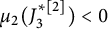 ), if and only if
$R_0>2$
 .
The proof can be found in the Appendix.
Different from a corresponding delay differential equation, it seems very difficult (if not impossible, see discussions in the final discussion section) to determine the sign of
$\mu _2(J_3^{[2]})$
 in the whole
$\mathbb {R}_+^3$
 , so we estimate a suitable region
$\Omega $
 , where
$\mu _2(J_3^{[2]})<0$
 according to Lemma 3.14.
Let
$\Delta I_i := I_i - I^*$
 for
$i=0,1,2$
 , and define
$ \theta := \|\Delta I\|_\infty = \max _{i=0,1,2} |\Delta I_i|$
 . We have the following result.
Lemma 4.5 Suppose that
$R_0>2$
 (ensuring
$k_*\in (1/2,1)$
 and
$\lambda _{\max }(S^*)<0$
 ). If
$\theta < \mathcal {G} $
 , then
$\mu _2(J^{[2]}_3)<0$
 (equivalently,
$\lambda _{\max }(S_1)<0$
 ), where
$\mathcal {G}:=\min \{\theta ^*_1,\theta _2^*\}. $
 Here,
$\theta _1^*$
 and
$\theta _2^*$
 are the unique positive root in the interval
$(0,I^*)$
 of

and

respectively. The explicit expressions of
$C_I(\cdot ),\mathcal {B}(\cdot ), R_1^*(\cdot )$
 , and
$R_2^*(\cdot )$
 are given in (A.8), (A.9), (A.12), and (A.13), respectively.
We defer this important estimation to the Appendix. Based on Lemmas 3.14 and 4.5, we have the following theorem.
Theorem 4.6 Assume that
$R_0>2$
 . Then system (4.12) has no non-constant periodic solutions contained entirely in
$(I^*- \mathcal {G} ,I^*+ \mathcal {G} )^3$
 .
As a consequence, we have the following result for system (4.1).
Theorem 4.7 Assume that
$R_0>2$
 . If a nontrivial periodic solution
$I(t)$
 of system (4.1) is completely contained in
$(I^*-\mathcal {G},I^*+\mathcal {G})$
 , then its period cannot be
$3\tau $
 .
We also need to establish the lower and upper bounds to
$\beta (t)$
 .
Lemma 4.8 Given that
$R_0>1$
 and
$\tau>\tau ^*$
 . If the component of periodic solutions
$I(t)$
 of system (4.1) is restricted in the interval
$(I^*-\mathcal {G},I^*+\mathcal {G})$
 for any
$t\in R$
 , then there exist constants
$\beta _{-},\beta _{+}>0$
 , given by

and

such that
$\beta (t) \in (\beta _{-}, \beta _{+})$
 for all
$t\in [t_0,\infty )$
 , as long as
$\beta (s)\in (\beta _{-}, \beta _{+})$
 for all
$s\in [t_0-\tau ,t_0]$
 . Here,
$I_{-}:=I^*-\mathcal {G}$
 and
$I_{+}:=I^*+\mathcal {G}$
 . Moreover, as
$\mathcal {G}$
 decreases,
$\beta _{-}$
 increases and
$\beta _{+}$
 decreases, with
$\beta ^*\in (\beta _{-},\beta _{+})$
 . In particular, as
$\mathcal G\downarrow 0$
 , we have
$\beta _{-}\uparrow r$
 ,
$\beta _{+}\downarrow r$
 . Then
$|\beta (t)-r|<\max \{\beta _{+}-r,r-\beta _{-}\}$
 for all
$t\in [t_0-\tau ,\infty )$
 .
Proof Applying the relation
$I_{+}-I_{-}=2\mathcal {G}$
 and solving
$F(I_+\beta _+)=\beta _-$
 and
$F(I_-\beta _-)=\beta _+$
 gives

and

Define

Then
$U(0)=\beta ^*$
 ,
$\beta _{-}=U(\mathcal {G})$
 and
$\beta _{+}=U(-\mathcal {G})$
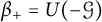 . Moreover,

Since

we conclude that
$U'(x)<0$
 for
$x\in [0,I^*)$
 . Therefore,
$\frac {d U(-x)}{dx}>0$
 for
$x\in [0,I^*)$
 . Hence,
$\beta _{-}<\beta _{+}$
 and
$\beta ^*\in (\beta _{-},\beta _{+})$
 .
We now prove
$\beta (t)\in (\beta _{-},\beta _{+})$
 for all
$t\geq t_0$
 . Fix
$t\in [t_0,t_0+\tau ]$
 , since
$I(t-\tau )\in (I_-,I_+)$
 and
$\beta (t-\tau )\in [\beta _-,\beta _+]$
 , we have

By strict monotonicity of
$F(\xi )$
 on
$[0,\infty )$
 , we obtain

Hence,
$\beta _-< \beta (t) < \beta _+$
 , for any
$t\in [t_0,t_0+\tau ]$
 . Repeating the above on successive intervals
$[t_0+n\tau ,t_0+(n+1)\tau ]$
 , we obtain
$\beta _-\ <\ \beta (t)\ <\ \beta _+$
 for all
$t\ge t_0$
 .
We can now obtain a range of plausible periodic solutions: Suppose
$R_0>2$
 . Then there exists
$\delta _{\mathcal {G}}>0$
 such that, for any fixed
$\tau \in (\tau ^*,\,\tau ^*+\delta _{\mathcal {G}}]$
 with
$\tau _M:=\tau ^*+\delta _{\mathcal {G}}$
 , for every periodic solution of system (4.1) with period
$T$
 satisfying
$2\tau <T<3\tau $
 , denoted as
$E(t;\tau ,T):=(I(t;\tau ,T),\beta (t;\tau ,T))$
 ,
$I(t;\tau ,T)\in \left [ I^*-\mathcal {G},\ I^* +\mathcal {G} \right ]$
 holds (see Figure 2-(b)). This statement about the range of plausible periodic solutions can be easily shown by way of contradiction. Assuming otherwise, for any
$\delta $
 , there is some
$\tau _{\delta }\in (\tau ^*,\tau ^*+\delta )$
 , such that system (4.1) admits a
$T$
 -periodic solution
$I(t;\tau _\delta ,T)$
 , for which there is a time
$t_s\in R$
 such that
$I(t_s)=I_{+}$
 ,
$I'(t_s)>0$
 and
$I(t)\in (I_-,I_+)$
 for all
$t\in [-\tau ,t_s]$
 , then
$\beta (t)\in (\beta _{-},\beta _{+})$
 for all
$t<t_s$
 from Lemma 4.8. Hence,
$\beta (t_s)>r$
 due to
$I'(t_s)>0$
 . Let
$\delta _n:=1/n$
 , for every
$n$
 , there is some
$\tau _{n}\in (\tau ^*,\tau ^*+\delta _n)$
 , and there exists a
$T_n$
 periodic solution
$I_n(t)$
 with
$T_n\in (2\tau _n,3\tau _n)$
 , there exists
$t_{s,n}$
 such that
$I_n(t_{s,n})=I_{+}$
 ,
$I_n'(t_{s,n})> 0$
 , and
$ I_n(t)<I_{+}$
 for all
$s<t_{s,n}$
 . Consequently, from
$I^{\prime }_n(t)=(\beta _n(t)-r)I_n(t)$
 with
$I_{+}>0$
 , we have
$\beta _n(t_{s,n})> r$
 . Note that
$\beta _n(t_{s,n}+\tau _n)=f(\beta _n(t_{s,n}),I_n(t_{s,n}))=f(\beta _n(t_{s,n}),I_+)\le f(r,I_+). $
 Therefore,
$ \beta ^*-\beta _n(t_{s,n}+\tau _n)\ \ge F(rI^*)- F(r I_+). $
 Using the mean value theorem, there exists
$\xi \in [rI^*,rI_+]$
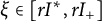 such that

since
$-F'(x)$
 decreases on
$[0,\infty )$
 . Hence,
$ \big |\beta _n(t_{s,n}+\tau _n)-\beta ^*\big |\ \ge \big |(F'(rI_{+})\big | r \mathcal {G}$
 , a contradiction.
(a)
$\lambda _{\max }(S_1)$
 for all
$(I_0,I_1,I_2)$
 in the
$\theta $
 -neighborhood of equilibrium
$I^*$
 with
$\theta \in [0,I^*)$
 . The solid blue curve shows the maximum (“worst-case”) value of
$\lambda _{\max }(S_1)$
 over the grid for each fixed
$\theta \in [0,I^*)$
 . This numerical illustration shows that
$\lambda _{\max }(S_1)<0$
 holds for all
$I_0,I_1,I_2\in (I^*-0.951,I^*+0.951)$
 . (b) Periodic solution of (4.1) with amplitude in
$(I^*- \mathcal {G},I^*+ \mathcal {G})$
 ; here,
$\tau ^*=3.989327447$
 and
$\tau _e\approx 4.039$
 ,
$\frac {d\lambda }{d\tau }|_{\lambda =\omega i,\tau =\tau ^*}=0.04807979388-0.1740577i $
 . (c) Bifurcation diagram of the amplitude of
$I(t)$
 with respect to
$\tau $
 for system (4.1). For panels (a)–(c), the parameter values are
$\kappa =1.2$
 ,
$\beta _c=2$
 ,
$r=0.6$
 , and
$I^*=3.24074$
 . The corresponding value
$\lambda _{\max }(S^*)=-0.2856$
 and
$\mathcal {G}=0.2297436746<0.951$
 , and panel (a) numerically confirms Lemma. 4.5, showing that
$\lambda _{\max }(S_1)<0$
 for all
$I_0,I_1,I_2\in (I^*-\mathcal {G},\,I^*+\mathcal {G})$
 . (d). Periodic solution of (4.1) with amplitude in
$(I^*- \mathcal {G},I^*+ \mathcal {G})$
 , the parameter values are
$\kappa =0.005$
 ,
$\beta _c=2$
 ,
$r=0.6$
 ,
$I^*=777.778$
 ,
$\tau ^*=3.989327447$
 ,
$\mathcal {G}=55.192$
 , and
$\tau _e\approx 4.0166$
 .
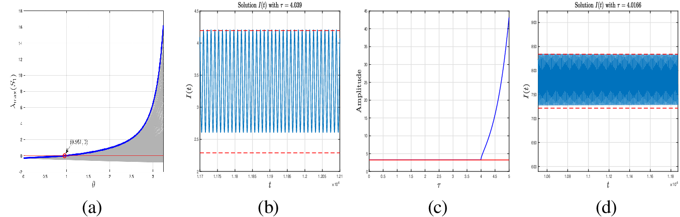
Figure 2 Long description
The figure consists of four panels labeled (a) to (d).
* Panel (a): A line graph with theta on the x-axis ranging from 0 to 3 and lambda sub max (S sub 1) on the y-axis ranging from -2 to 18. A solid blue curve increases exponentially. A red horizontal line marks y equals 0. A red circle at (0.951, 0) indicates an intersection point. A gray shaded region exists below the blue curve.
* Panel (b): A line graph titled Solution I(t) with tau equals 4.039. The x-axis is time t (multiplied by 10 super 4) and the y-axis is I(t). The data shows a high-frequency oscillation between approximately 2.6 and 4.2. Two red dashed horizontal lines mark the upper and lower bounds of the oscillation.
* Panel (c): A bifurcation diagram with tau on the x-axis from 0 to 5 and Amplitude on the y-axis from 0 to 45. A red horizontal line remains constant at an amplitude of approximately 3 until tau equals 4, where a blue curve branches upward, showing a sharp increase in amplitude.
* Panel (d): A line graph titled Solution I(t) with tau equals 4.0166. The x-axis is time t (multiplied by 10 super 4) and the y-axis is I(t). It shows a dense, high-frequency oscillation centered around 775, bounded by two red dashed horizontal lines at approximately 725 and 830.
Recall that
$C(I^*, \tau ^*, T^*)$
 is the connected component through
$(I^*, \tau ^*, T^*)$
 in
$\Sigma (\mathcal {F})$
 . We define

The local Hopf bifurcation theorem and the above discussion on the range of plausible periodic solutions ensure that the set defining
$\tau _e $
 is nonempty, and therefore
$\tau _e$
 is well defined. The value of
$\tau _e$
 could be infinity theoretically, but our simulations provided later indicate that after
$\tau ^*$
 , as
$\tau$
 increases, the amplitude of the periodic solution becomes so large that the periodic wave presents as a spike. These indicate the time delay is indeed the reason for onset of a large epidemic wave that susceptible populations will be depleted by the infection to a level that our standing assumption that susceptible remains relatively unchanged is no longer valid. Note also that while the expressions for
$\tau ^*$
 and
$\lambda _{\max }(S^*)$
 are independent of
$\kappa$
 , both
$I^* \text { and } \mathcal G$
 vary with
$\kappa$
 . Simulations reported in Figure 2-(b) and (d) show that
$ \tau _e $
 depends on
$ \kappa $
 , and small variation of
$ \kappa $
 can lead to larger values of
$ I^* $
 and
$\mathcal {G} $
 , resulting in smaller values of
$\tau _e $
 .
Theorem 4.9 Assume
$R_0>2$
 . Then for every
$\tau \in (\tau ^*, \tau _e)$
 , system (4.1) has a non-constant periodic solution with period in
$(2\tau , 3\tau )$
 .
Proof We first note that the projection of
$ C(I^*, \tau ^*, T^*)$
 onto the
$\tau $
 -space must be bounded below by
$\tau ^*$
 . We now claim that this projection must contain
$(\tau ^*, \tau _e)$
 . By way of contradiction, and since we have shown that
$C(I^*, \tau ^*, T^*)$
 is unbounded, there must be the first
$\tilde \tau \in (\tau ^*, \tau _e)$
 so that we can find a sequence of
$\tau ^{(n)}\to \tilde \tau $
 from below as
$n\to \infty $
 such that system (4.1) has a nontrivial
$p^{(n)}$
 -periodic solution
$(\beta ^{(n)}(t), I^{(n)}(t))$
 at
$\tau =\tau ^{(n)}$
 for each
$n=1,2,\ldots $
 such that either (i)
$\sum _{t\in R}\beta ^{(n)}(t)+\sum _{t\in R}I^{(n)}(t) \to \infty $
 or (ii)
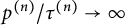
$p^{(n)}/\tau ^{(n)}\to \infty $
 . By definition of
$\tau _e$
 and since
$\tilde \tau <\tau _e$
 , we know that
$|I^{(n)}(t)-I^*|\le \mathcal {G}$
 for all
$t\in R$
 . This, by Lemma 4.8, also implies that
$|\beta ^{(n)}(t)-r|\le \max \{\beta _+-r, r-\beta _-\}$
 for all
$t\in R$
 . So (i) does not hold. By Theorem 4.6, we have also
$p^{(n)}/\tau ^{(n)}\in (2, 3)$
 for all
$n=1, 2, \ldots $
 , so (ii) cannot hold. This proves the claim that this projection must contain
$(\tau ^*, \tau _e)$
 , completing the proof.
We conclude this section with a note that if
$\tau _e>\tau _k$
 for some
$k\ge 1$
 , then a similar argument can be used to show that the projection of
$C(I^*, \tau _k, T^*)$
 onto the
$\tau $
 -space contains
$(\tau _k, \tau _e)$
 , and hence the existence of a fast oscillating periodic solution can also be established for
$\tau \in (\tau _k, \tau _e)$
 .
5 Discussion and conclusions
We have used a recently developed epidemic-behavioral model with delay to motivate our development of a global Hopf bifurcation theory for a general delay-algebraic system. Our strategy is to convert such a delay-algebraic system into a functional differential equation with infinitely many integer multiples of the delay, and then use the
$S^1$
 -degree-based global Hopf bifurcation theory for two-parameters parameterized functional differential equations with infinite delay. We have also used the epidemic-behavioral model to illustrate how our global bifurcation theory can be applied to examine the global continuation of periodic solutions bifurcated locally through the Hopf bifurcation mechanism in general delay-algebraic systems.
Similarly to the established procedure of applying the equivalent degree-based global Hopf bifurcation theory to delay differential equations, we need to 1) obtain uniform bounds for possible periodic solutions and 2) establish uniform bounds of the periods of periodic solutions (alternatively, bounds for the ratio of periods over delays), and this may be achieved by ruling out periodic solutions of the delay-algebraic system with a certain prescribed period. Unfortunately, this procedure presents substantial challenges due to the hybrid nature of the delay-algebraic system. In particular, the discrete component, the algebraic subsystem, renders existing techniques ineffective: uniform bounds for periodic solutions can hardly be achieved. As illustrated in Figure 1-(c),
$I(t)$
 components can be very close to zero while its peaks can be very large, with no uniform upper bound or positive lower bound observed when varying the delay. In addition, ruling out periodic solutions of an equivalent ordinary differential system is difficult, since the ordinary differential system (even when in the simplest case with dimension 3) has both a competitive nature and embedded predator–prey loops.
We are thus forced to establish the existence of the most interesting periodic solutions (slow oscillations) not for all time delays larger than the first critical value
$\tau ^*$
 (for Hopf bifurcation to occur) but rather for an interval of
$(\tau ^*, \tau _e)$
 . The choice of
$\tau _e$
 is determined by the determination of a neighborhood of the relevant equilibrium (in our case, the disease-established and behavior-balanced equilibrium
$(I^*,\beta ^*)$
 , where we can rule out nontrivial periodic solutions of the equivalent ordinary differential system). In particular, Theorem 4.6 identifies a neighborhood
$(I^*-\mathcal {G},I^*+\mathcal {G})^3$
 of the equilibrium point
$(I^*,I^*,I^*)$
 within which non-constant periodic solutions can be excluded using the Li–Muldowney technique of compound matrix [Reference Li and Muldowney28]. This is shown in our numerical simulations presented below with
$\kappa =1.2$
 ,
$\beta _c=2$
 , and
$r=0.6$
 . For these choices of parameter values, we have
$\mathcal {G}=0.2297436746$
 by Theorem 4.7 (see Figure A2-(a) in the Appendix). This result is not optimal mathematically: as shown in Figure 2-(a),
$\mu _2(J^{[2]}_3)<0$
 (to ensure the
$3\tau $
 - periodic solution can be ruled out) holds for a larger range
$(I^*-0.951, I^*+0.951)^3$
 . As shown in our numerical simulations (see Figure 3), the non-existence of non-constant periodic solutions of the ordinary differential system occurs over a larger parameter range and a large neighborhood of the equilibrium. Note that while the beginning of an epidemic spike appears in the real world epidemic setting (within 90 days since the beginning of the epidemic wave takes off), the epidemic wave presents itself as a spike in the sense that after a short-term transition the number of infections increases rapidly to a level that our model assumption that susceptible population remains relatively unchanged is no longer valid, only under such an assumption periodic solutions with large amplitudes appear. In short, our theoretical results should be interpreted as that nonlinear oscillations as periodic waves will emerge after the delay passing through a critical value, and this observed oscillatory pattern around the nontrivial equilibrium will persist when the delay is further increased. Large delay will lead to an epidemic spike in short term that is part of a long-term oscillatory pattern. Figure 2-(b)–(d) numerically illustrates Theorem 4.9, for the range given in Theorem 4.7, there will be a
$\tau _e>\tau ^*$
 , such that
$I(t)$
 within
$\left [ I^*-\mathcal {G},\ I^* +\mathcal {G} \right ]$
 as long as
$\tau \in (\tau ^*, \tau _e)$
 . Deriving an explicit expression for
$\tau _e$
 remains a challenging problem for future studies.
The trajectories of system (4.12):
$\gamma (t)$
 (red),
$\sigma (\gamma (t))$
 (blue), and
$\sigma ^2(\gamma (t))$
 (green). (a) Initial condition is
$(I_0(0),I_1(0),I_2(0))=(20, 20.5, 2)$
 . (b) Initial condition is
$(I_0(0),I_1(0),I_2(0))=(2000, 20, 2)$
 .
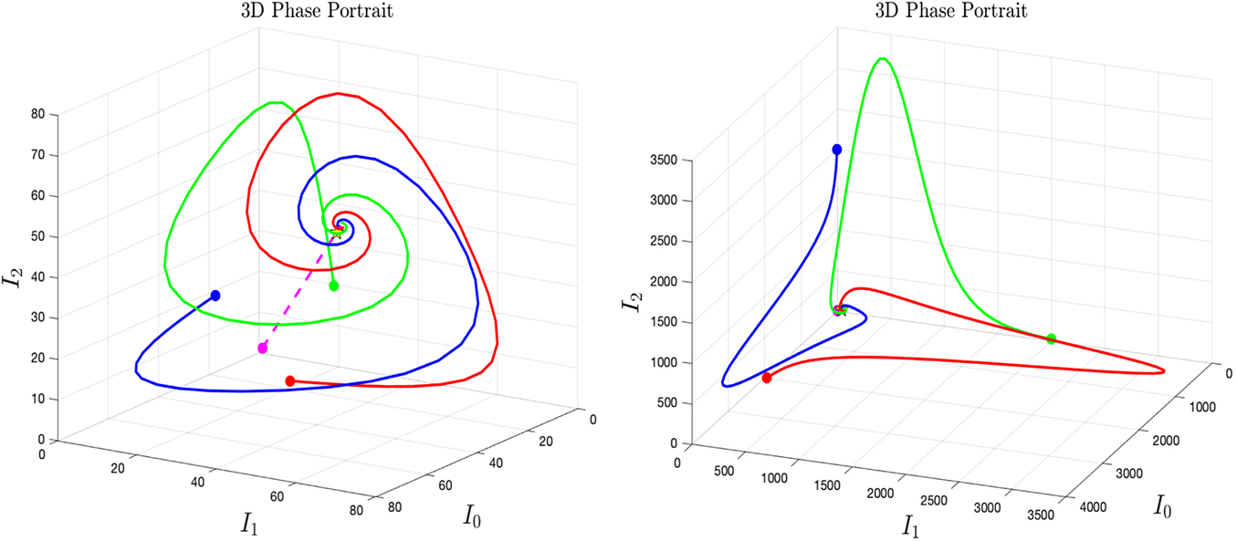
Figure 3 Long description
Two 3 D phase portraits titled 3 D Phase Portrait are arranged side-by-side. Both plots use axes labeled I sub 0, I sub 1, and I sub 2.
Panel a on the left shows a coordinate space ranging from 0 to 80 on all axes. Three trajectories begin at distinct points marked by solid dots. The red trajectory starts near the I sub 0 axis, the blue trajectory starts at a mid-range point, and the green trajectory starts higher up. All three lines follow a wide, outward-curving path before spiraling inward toward a common central equilibrium point. A dashed magenta line connects the starting region to the center.
Panel b on the right shows a much larger coordinate space ranging from 0 to 4000 on all axes. The trajectories (red, blue, and green) start at much higher initial values. They exhibit sharp, triangular-like loops that extend far into the coordinate space before rapidly converging and spiraling tightly into a central equilibrium point located near the origin relative to the scale of the axes. The green trajectory shows the most significant vertical peak on the I sub 2 axis before descending into the spiral.
A Appendix
A.1 A proof of Proposition 3.6
Proof If
$ I_0(0) = I_1(0)=\dots = I_{n-1}(0) $
 , then by symmetry of the system when
$ I_0 = I_1=\dots =I_{n-1} $
 , we have

Thus, the diagonal
$\mathcal {D}_n$
 is invariant.
Function
$\mathcal {B}(x)$
 with
$x\in (-I^*,I^*)$
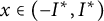 . Parameter values are:
$\kappa =1.2$
 ,
$\beta _c=2$
 ,
$r=0.6$
 , and
$I^*= 3.24074$
 .

Figure A1 Long description
The x-axis ranges from negative 3 to 3, and the y-axis, labeled B of x, ranges from 0 to 2. A solid blue curve descends from the top-left to the bottom-right.
* At the far left, a blue circle at x equals negative 3.24 and y equals 2 is labeled with an arrow pointing to the limit as x approaches I super star of B of negative x.
* In the center, a red circle at x equals 0 and y equals 0.6 is labeled with an arrow pointing to B of 0.
* At the far right, a green circle at x equals 3.24 and y equals 0.13 is labeled with an arrow pointing to B of I super star.
The curve exhibits a convex shape, decreasing more rapidly at negative x values and flattening as it approaches the positive x boundary.
A.2 A proof of Proposition 3.7
Proof Let
$ \tilde {I}_j := I_{j+1 \bmod n}(t) $
 . Then

As
$ \tilde {I}_j = I_{j+1 \bmod n}$
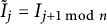 ,
$\tilde {I}_{j+1 \bmod n} = I_{j+2 \bmod n}, \dots $
 ,
$\tilde {I}_{j+n-1 \bmod n} = I_j $
 , we can rewrite

which shows that
$ \tilde {\gamma } (t):= (\tilde {I}_0(t), \tilde {I}_1(t), \tilde {I}_2(t)\ldots ,\tilde {I}_{n-1}(t) ) = \sigma (\gamma (t)) $
 is also a solution to system (3.5).
A.3 A proof of Proposition 3.8
Proof We consider
$n=3$
 , the general case can be shown similarly. System (3.5) becomes

Note that
$ \Phi _{(1,2)}(I_0, I_1, I_2) = (\tilde {I}_0, \tilde {I}_1, \tilde {I}_2) := (I_0, I_2, I_1) $
 . Substituting into the original system gives

which has the same structure as system (A.1), with an appropriate relabeling of the variables.
A.4 A proof of Lemma 4.4
Proof The Jacobian matrix
$J_3$
 associated with a general periodic solution of system (4.12) given by (4.13) can be simplified as

Denote
$k_*:=1-1/R_0$
 . Setting
$I_0=I_1=I_2=I^*$
 yields

and

Therefore,

By direct calculation, we have

and

Then

Eigenvalues of
$S^*$
 are

with
$0<k_*<1$
 . Obviously,
$\lambda _{\max }\{S^*\}=\lambda _1$
 . Hence,
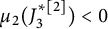
$\mu _2(J_3^{*[2]})<0$
 if and only if
$k_*>1/2$
 , that is,
$R_0>2$
 .
A.5 A proof of Lemma 4.5
Proof According to Lemma 3.13, we have
$\beta _1=f(\beta _0,I_0)$
 ,
$\beta _2=f(\beta _1,I_1)$
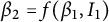 , and
$\beta _0=f(\beta _2,I_2)$
 . Then after simplifying
$k_{i}$
 , we get

Denote
$B_i:=\beta _i I_i$
 and
$Y_i := \frac {\kappa B_i}{1 + \kappa B_i}=1-\frac {\beta _{i-1}}{\beta _c}>0.$
 Simple calculations give

and
$\alpha =1 + Y_0 Y_1 Y_2$
 .
Then the Jacobian matrix
$J_3$
 given by (A.2) can be simplified as

The second additive compound matrix of
$J_3$
 is as follows:

Since
$\mu _2(J_3^{[2]})=\mu _2( S_0/\alpha )=\frac {1}{\alpha }\lambda _{\max }\big ( \frac {S_0+ S_0^{\top }}{2}\big )=\frac {1}{\alpha }\lambda _{\max }\big ( S_1\big )$
 and
$\alpha>0$
 , we have
$\operatorname {Sign}(\mu _2(J_3^{[2]}))=\operatorname {Sign}(\lambda _{\max }\big ( S_1\big ))$
 . Next, we estimate the neighborhood of
$(I_0,I_1,I_2)$
 around
$I^*$
 for which
$\lambda _{\max }\big ( S_1\big )<0$
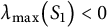 .
By direct calculation, we have

and the symmetric matrix
$S_1$
 :

Denote
$Y^* :=1-\frac {\beta ^*}{\beta _c}$
 ,
$\Delta \beta _i := \beta _i - \beta ^*$
 ,
$\Delta Y_i := Y_i - Y^* =\; -\frac {\Delta \beta _{\,i-1}}{\beta _c}$
 ,
$\Delta (I_i/I_j) :=\frac {I_j}{I_j}-1 $
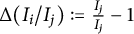 , and

Since
$\Delta (I_i/I_j) = \tfrac {I^*+\Delta I_i}{I^*+\Delta I_j} - 1 = \tfrac {\Delta I_i - \Delta I_j}{I^*+\Delta I_j}$
 , we obtain

for
$i,j\in \{0,1,2\}$
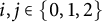 with
$0\leq \theta <I^*$
 .
$C_I(\theta )$
 is increasing in
$\theta \in (0,I^*)$
 .
Denote
$\Delta \beta _{\max } :=\|\Delta \beta \|_\infty = \max _{i=0,1,2}|\Delta \beta _i|.$
 We obtain

Next, we need to identify the bound of
$\Delta \beta _{\max } $
 when
$I_0,I_1,I_2\in (I^*-\theta ,I^*+\theta )$
 with
$\theta \in [0,I^*)$
 .
Denote

where
$x\in (-I^*,I^*)$
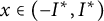 and
$H(x_1,x_2,x_3)$
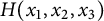 is given by (4.10).
By Corollary 3.2-(ii), it follows that
$\mathcal {B}(x)$
 is decreasing function of
$x\in (-I^*,I^*)$
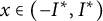 and
$0<\mathcal {B}(\theta )\leq \beta _i\leq \mathcal {B}(-\theta )$
 . Hence,

where
$\mathcal {B}(0)=H_{[\infty ]}(I^*)=r$
 . Clearly,
$\mathcal {B}(-\theta )-r$
 is increasing in
$\theta $
 . Further,

and
$\lim _{x\to I^*}\mathcal {B}(-x)=\beta _c$
 (see Figure A1 for a graphical illustration).
The functions
$R_1^*(r-\mathcal B(\theta ))+C_I(\theta )R_2^*(r-\mathcal B(\theta ))$
 and
$R_1^*(\mathcal B(-\theta )-r)+C_I(\theta )R_2^*(\mathcal B(-\theta )-r)$
 for
$\theta \in [0,I^*)$
 . (a) Parameter values:
$\kappa =1.2$
 ,
$\beta _c=2$
 , and
$r=0.6$
 , yielding
$I^*=3.24074$
 ,
$R_0\approx 3.33$
 , and
$\lambda _{\max }(S^*)=-0.2856$
 . The corresponding intersection points are
$\theta _1^*=0.2459386271$
 and
$\theta _2^*=0.2297436746$
 , and hence
$\mathcal G=\theta _2^*=0.2297436746$
 . (b) Enlarged view of panel (a) near the intersections. (c) Parameter values:
$\kappa =0.005$
 ,
$\beta _c=2$
 , and
$r=0.6$
 , with
$\lambda _{\max }(S^*)=-0.2856$
 . The corresponding equilibrium value is
$I^*=777.78$
 , and the intersection points are
$\theta _1^*=58.994$
 and
$\theta _2^*=55.192$
 , yielding
$\mathcal G=\theta _2^*=55.192$
 .

Figure A2 Long description
A three-panel figure labeled a, b, and c.
Panel a: A line graph with theta on the x-axis from 0 to 3.5 and a vertical axis from 0 to 200. Two curves, one blue and one orange, start near the origin and increase exponentially. The orange curve is consistently above the blue curve. Both curves approach a vertical dashed asymptote at theta equals I super star, which is approximately 3.24.
Panel b: An enlarged view of panel a focusing on the theta range 0.16 to 0.32 and vertical range 0.15 to 0.45. A horizontal dashed line labeled y equals minus lambda sub max of S super star is positioned at approximately 0.285. The blue and orange curves from panel a appear as nearly linear diagonal lines. The orange curve intersects the horizontal dashed line at theta sub 2 super star equals 0.2297, and the blue curve intersects it at theta sub 1 super star equals 0.2459.
Panel c: A line graph with theta on the x-axis from 10 to 110 and a vertical axis from 0 to 1. A horizontal dashed blue line represents minus lambda sub max of S super star at 0.2856. Two diagonal lines, one purple and one green, intersect the horizontal line. The purple line intersects at theta sub 2 super star equals 55.192, marked with a small square. The green line intersects at theta sub 1 super star equals 58.994, marked with a small circle.
Define the symmetric matrix

where

and

By Weyl’s inequality for a symmetric matrix, we obtain
$ \lambda _{\max }(S_1) \le \lambda _{\max }(S^*)+\lambda _{\max }(\Delta S_1) \le \ \lambda _{\max }(S^*)+\|\Delta S_1\|_\infty .$

Next, we estimate
$ \|\Delta S_1\|_\infty $
 . By direct calculation, we obtain

A similar lengthy calculation yields

Next, we estimate elements of every entry of
$\Delta S_1$
 . By calculating, we obtain

and

where
$C_{\beta 1}$
 and
$C_{\beta 2}$
 are positive and only depend on the equilibrium value
$I^*$
 .
Similarly, we obtain

Then we have

with

and

Denote
$b:=\frac {\beta ^*}{\beta _c}$
 , then
$Y^*=1-b$
 . Since
$\beta ^*=r$
 ,
$b=1/R_0=1-k_*$
 , and
$k_*=Y^*$
 . Given that
$R_0>2$
 (i.e.,
$b\in (0,1/2)$
 and
$k_*>1/2$
 ), one obtains


and


Obviously,
$R_1^*(x)$
 and
$R_2^*(x)$
 are polynomial functions of
$x$
 with all coefficients being nonnegative, therefore, both
$R_1^*(x)$
 and
$R_2^*(x)$
 are increasing in
$x>0$
 . Therefore, if follows from (A.10) that

For
$\theta \in [0,I^*)$
 ,
$\lambda _{\max }\big (S_1\big )<0$
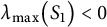 is sufficiently ensured by

Both
$R^*_1(r-\mathcal {B}(\theta ))+C_I(\theta )R_2^*(r-\mathcal {B}(\theta ))$
 and
$R^*_1(\mathcal {B}(-\theta )-r)+C_I(\theta ) R_2^*(\mathcal {B}(-\theta )-r)$
 are continuous and increasing in
$\theta $
 (see Figure A2-(a)). Since

and


there must exist unique values
$\theta ^*_1\in (0,I^*)$
 and
$\theta ^*_2\in (0,I^*)$
 such that

and

respectively (see Figure A2-(b,c)). Moreover,

and

Let
$\mathcal {G}=\min \{\theta _1^*,\theta _2^*\}$
 . Therefore, for any
$I_0,I_1,I_2\in (I^*-\mathcal {G},I^*+\mathcal {G})$
 , it holds that
$\lambda _{\max }\big ( S_1\big )<0$
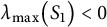 and
$\mu _2(J^{[2]}_3)<0$
 .
Data availability statement
All data supporting the findings of this study are provided within the article.
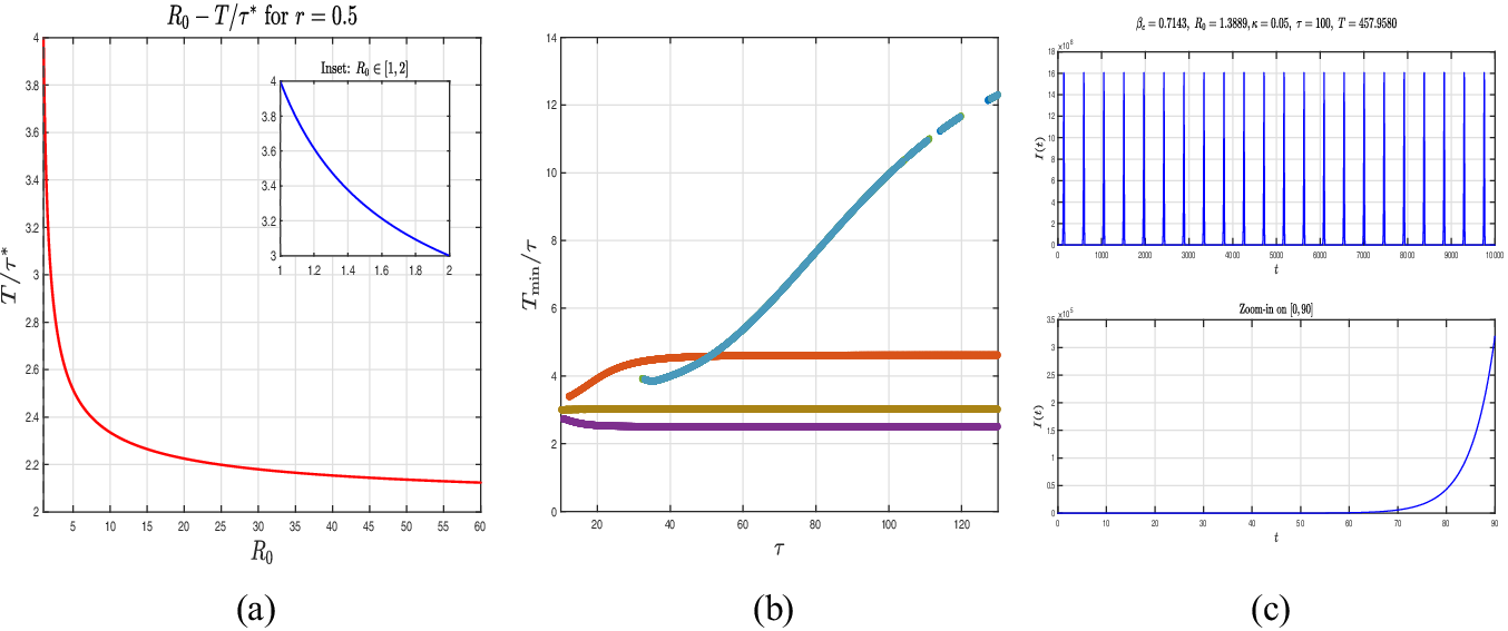


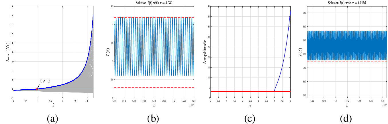


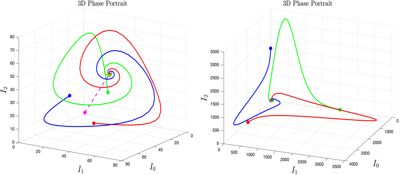


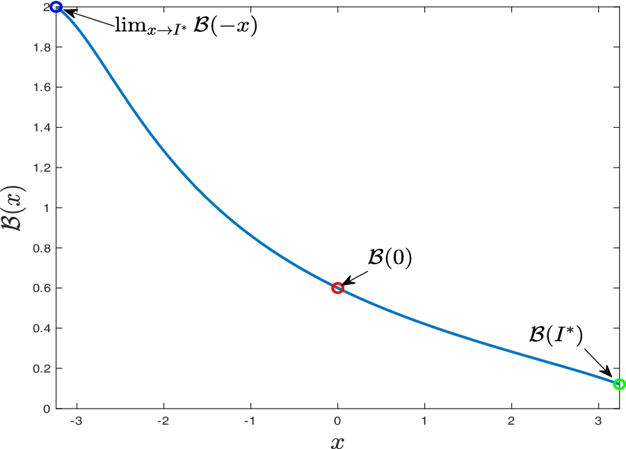


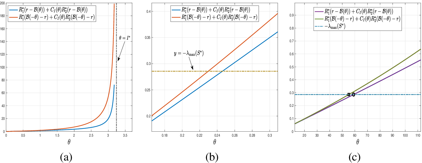


 Open access

