1 Introduction
Under classic linear water wave theory, when a regular train of small steepness incident waves meets a vertical wall it is entirely reflected, setting up a standing wave field. However, the problem becomes significantly more complicated when the wall is truncated to form a step that allows the incident waves to overwash the step, i.e. force a shallow-water flow on the step. As will be shown, the interfacial region where the water flows onto the step is characterised by vortices, overturning and air entrainment, implying the need for a computational fluid dynamics (CFD) modelling approach. A short distance along the step, the overwash transitions into a nonlinear shallow-water flow, driven by fast-travelling bores carrying vortices created by wave breaking.
The overwash phenomenon is common in wave interactions with thin floating plates – the standard model of ocean wave interactions with sea ice floes – due to the small freeboards of the plates. It has been noted predominantly in laboratory experiments, initially by Montiel et al. (Reference Montiel, Bennetts, Squire, Bonnefoy and Ferrant2013a ,Reference Montiel, Bonnefoy, Ferrant, Bennetts, Squire and Marsault b ) whilst studying the elastic response of a plastic disk to regular waves, and recently by Sree, Law & Shen (Reference Sree, Law and Shen2017) whilst studying wave propagation along a viscoelastic plate. In both cases, vertical barriers were installed around the edges of the plates to prevent overwash and improve agreement with linear models. Yiew et al. (Reference Yiew, Bennetts, Meylan, French and Thomas2016) compared the hydrodynamic responses of disks with and without edge barriers, showing that the response amplitude operators (RAOs) of the disk without barriers can decrease as the incident wave steepness increases, which is when overwash becomes more pronounced, whereas the RAOs for the disk with barriers are insensitive to incident steepness. Similarly, McGovern & Bai (Reference McGovern and Bai2014) noted overwash of thin plates during laboratory experiments, and attributed smaller than expected RAOs to the overwash.
Impacts of overwash on wave transmission by thin plates have been investigated experimentally in a series of related papers. Bennetts et al. (Reference Bennetts, Alberello, Meylan, Cavaliere, Babanin and Toffoli2015) studied transmission of regular incident waves of length 0.56–1.51 m and amplitude
 ${\sim}4{-}36~\text{mm}$
by a
 $1~\text{m}\times 1~\text{m}$
square plate of thickness 5–20 mm, without barriers. They used a video camera to record the overwash and a probe mounted on the plate to measure the overwash depth, from which it can be inferred that the Reynolds number is
 ${<}2000$
, based on the time averaged depth and velocity of bores in the overwash. A correlation was noted between the irregularity of the transmitted wave field and the overwash becoming deeper (up to
 ${\sim}10~\text{mm}$
at the probe) and more energetic (judged by its significant wave height), which was partly attributed to overwash running off the plate and generating high frequency waves in the surrounding open water. Bennetts & Williams (Reference Bennetts and Williams2015) studied transmission of regular incident waves by arrays of 40–80 wooden disks, and found that the proportion of incident wave energy transmitted by the disks decreased when the incident wave amplitude was increased and the overwash became deeper and more energetic. Toffoli et al. (Reference Toffoli, Bennetts, Meylan, Cavaliere, Alberello, Elsnab and Monty2015) used essentially two-dimensional experiments (uniform in one horizontal direction) to show that the proportion of incident wave energy transmitted by a freely floating plastic plate decreases as incident wave steepness increases, and that the decreasing transmission correlates with energy dissipation. They attributed the energy dissipation to wave breaking in the overwash when bores generated at the leading and trailing edges of the plate collide, or simply that the incident wave energy forced into the overwash does not return to the reflected or transmitted wave fields. Nelli et al. (Reference Nelli, Bennetts, Skene, Monty, Lee, Meylan and Toffoli2017) extended this investigation, showing that the reduced transmission and energy dissipation are exacerbated if the plate is moored, such that the overwash becomes stronger, and are eliminated if edge barriers are used to prevent overwash.
In work closely related to the present study, Skene et al. (Reference Skene, Bennetts, Meylan and Toffoli2015) mathematically modelled overwash of a thin floating plate, using two-dimensional (one horizontal dimension and one depth dimension) linear potential-flow theory to model the plate and surrounding wave field (based on the findings of Meylan et al. Reference Meylan, Bennetts, Cavaliere, Alberello and Toffoli2015), which forces overwash modelled using one-dimensional (depth averaged) nonlinear shallow-water theory. The model extends the canonical model of wave–floe interactions, meaning it can readily be integrated into models of wave propagation through large fields of floes (e.g. Bennetts & Squire Reference Bennetts and Squire2012). They compared predictions of overwash depths to the point measurements collected during the experiments reported by Bennetts et al. (Reference Bennetts, Alberello, Meylan, Cavaliere, Babanin and Toffoli2015), finding that model outputs are accurate for small incident wave steepnesses, but increasingly overpredict depths as the steepness increases. The overpredictions were attributed to the not modelled processes of bore turbulence, wave breaking in the overwash and bore collisions. However, the complexity of the problem, in which the plate motion is coupled to the surrounding wave field, and overwash is forced from the leading and trailing ends of the plate, combined with only point measurements of overwash depths from the experiments, meant that the dominant mechanisms causing the discrepancies were not identified.
A larger (although still relatively modest) literature exists on modelling the cognate phenomenon of green water on ships, in which isolated extreme waves force water onto the surface of floating bodies with large freeboards, typically in the context of predicting hydrodynamic loads imposed on ship decks with complicated bow geometries. Mizoguchi (Reference Mizoguchi1988) pioneered green water modelling, using laboratory experiments on scaled ship decks, and a two-dimensional numerical model. The numerical model used the shallow-water equations to model the green water, and experimentally determined water depths around the ship deck as boundary conditions. Mizoguchi (Reference Mizoguchi1988) found the model predicts qualitatively, although not necessarily quantitatively, similar water depths along the deck to those founds in his experiments.
Buchner (Reference Buchner2002) and Greco, Faltinsen & Landrini (Reference Greco, Faltinsen and Landrini2005), Greco, Colicchio & Faltinsen (Reference Greco, Colicchio and Faltinsen2007) also used laboratory experiments to study green water forced by short duration wave packets, with peak amplitudes exceeding the freeboard by
 ${>}0.1~\text{m}$
. Buchner (Reference Buchner2002) used a freely floating model ship (floating production storage and offloading, FPSO), including complex bow geometries that was subjected to both regular and irregular waves. Greco et al. (Reference Greco, Faltinsen and Landrini2005, Reference Greco, Colicchio and Faltinsen2007) used a fixed, flat model ship deck subjected to a small wave train of
 ${\sim}4$
wave peaks generated by a flap-type wave maker (described in detail in the PhD thesis by Greco Reference Greco2001). In both sets of experiments, green water was found to be generated by plunging wave breaking motion over the edge of the deck, resulting in overturning, air entrainment and three-dimensional turbulent effects, and only developing into a shallow-water flow, with depths generally
 ${>}100~\text{mm}$
, as it propagates along the deck (the Reynolds numbers in the experiments can be inferred to be
 ${>}10^{4}$
). Similar effects were found as the green water collided with objects on the model ship deck. Therefore, Buchner (Reference Buchner2002) and Greco et al. (Reference Greco, Faltinsen and Landrini2005, Reference Greco, Colicchio and Faltinsen2007) deduced that a shallow-water model, of the form proposed by Mizoguchi (Reference Mizoguchi1988), was not sufficient to model green water at the edge of the deck or as it collided with on-deck structures.
Buchner (Reference Buchner2002) discussed the applicability of a range of potential green water models, and adopted a two-dimensional CFD modelling approach forced by an experimentally determined constant initial water height at the deck edge (similar to Mizoguchi Reference Mizoguchi1988). His model was based on the single-phase (water), incompressible Navier–Stokes equations, thus capturing both wave overturning at deck edge and shallow-water flow farther along the deck, solved with a volume of fluid method, and without a turbulence closure (i.e. the model assumed laminar conditions) or surface tension. Model predictions were shown to agree reasonably well, both qualitatively and quantitatively, with the experimental measurements, in terms of free surface profiles and depth signals measured along the deck, including close to the deck edge, where the free surface experiences the most pronounced overturning. Greco et al. (Reference Greco, Colicchio and Faltinsen2007) developed a two-dimensional model of the green water and surrounding basin of deeper water with forcing wave packets (generated by a virtual wave maker), based on a domain decomposition strategy, in which fully nonlinear potential-flow theory was used to model the majority of the flow, and the incompressible Navier–Stokes equations were used close to the deck edge during overturning events. The model was shown to provide better agreement with measured free surface profiles at the deck edge and in the shallow-water flow along the deck than the model used by Buchner (Reference Buchner2002), presumably due, at least in part, to modelling of the surrounding waves and because the model ship deck was held stationary.
Subsequent green water studies have predominantly employed CFD modelling techniques, particularly the use of the incompressible, laminar Navier–Stokes equations (as in Buchner Reference Buchner2002). Nielsen & Mayer (Reference Nielsen and Mayer2004) modelled the basin and green water (similar to Greco et al. Reference Greco, Colicchio and Faltinsen2007) using the single-phase, incompressible Navier–Stokes equations, solved using the volume of fluid method (similar to Buchner Reference Buchner2002), with a significantly more refined mesh than Buchner (Reference Buchner2002). They compared model predictions with experimental data presented by Buchner (Reference Buchner2002) and Greco et al. (Reference Greco, Faltinsen and Landrini2005, Reference Greco, Colicchio and Faltinsen2007). They found strong agreement (comparable to Greco et al. Reference Greco, Colicchio and Faltinsen2007) in terms of the free surface profile as waves overturn onto the deck, and in terms of the depth signals along the deck at times when air entrainment and turbulence were observed in the experiments.
In the present study, a finite-volume-based CFD method is used to analyse overwash of a step by small steepness incident waves, where the upper surface of the step is collinear with the undisturbed free surface of the water, and to assess the validity of modelling overwash using the approach of Skene et al. (Reference Skene, Bennetts, Meylan and Toffoli2015). The CFD model is two-dimensional and is based on the two-phase (water and air, thus modelling the dynamics of entrained air), laminar, incompressible Navier–Stokes equations, without surface tension. It is solved using the volume of fluid method on an unstructured mesh in the open-source CFD toolbox OpenFOAM (Weller et al. Reference Weller, Tabor, Jasak and Fureby1998). OpenFOAM has been used successfully to model wave breaking and wave interactions with fixed bodies (Higuera, Lara & Losada Reference Higuera, Lara and Losada2013a ,Reference Higuera, Lara and Losada b ), and the hydrodynamics of thin floating bodies in wave tank experiments (Bai, Zhang & McGovern Reference Bai, Zhang and McGovern2017). The laminar, no surface tension, incompressible CFD methodology used is similar to that of Nielsen & Mayer (Reference Nielsen and Mayer2004) and others, which were shown to predict accurately green water flows with Reynolds numbers orders of magnitude greater than in overwash.
Simulations are run for the same incident wave periods and a similar steepness range, as in the tests Skene et al. (Reference Skene, Bennetts, Meylan and Toffoli2015) analysed, resulting in similar overwash depths (
 ${<}20~\text{mm}$
) and similar Reynolds numbers (
 ${<}2000$
, based on time averaged depths and velocities), but does not produce breaking induced by bore collisions. Similar to Skene et al. (Reference Skene, Bennetts, Meylan and Toffoli2015), a mathematical model is developed in which overwash is modelled using nonlinear shallow-water theory, where the overwash is on top of the step rather than on a floating plate, and linear potential-flow theory is used to model the relatively deep water that forces overwash, in this case in a basin on one side of the step rather than on both sides of and beneath the plate. Applying the model to the relatively simple step problem, without the complications of a freely floating body and with overwash generated at one interface only, and assessing model performance using a CFD model (which provides high-resolution data on, e.g. depth and velocity fields, as opposed to experimental data with only depth measurements at a single point), provides deeper insights into model capabilities, as compared to Skene et al. (Reference Skene, Bennetts, Meylan and Toffoli2015). The model is shown to predict markedly different overwash depths and velocities with respect to the CFD model around the step front, as expected, but to predict similar depths and velocities once bores have formed along the step. The agreement is attributed to underlying agreement between mass and energy fluxes, which is shown to hold along the step, including points close to the step front, and a rapid transition to shallow-water flow after the water breaks onto the step.
2 CFD model
2.1 Model description
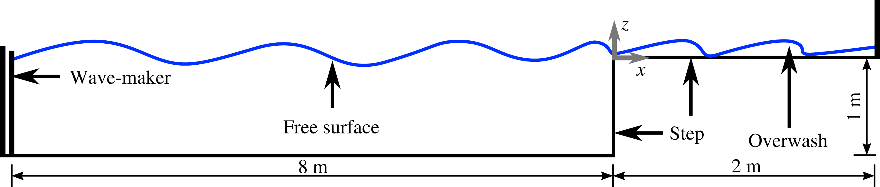
Consider a two-dimensional rectangular wave basin, with depth
 $H=1~\text{m}$
and length 8 m. A wave maker bounds the left-hand end of the basin and the vertical, front surface of a rectangular step bounds its right-hand end. Locations are defined using the Cartesian coordinate system
 $(x,z)$
, with origin at the upper vertex of the step. The horizontal coordinate,
 $x$
, points along the upper surface of the step, and the vertical coordinate,
 $z$
, points upwards.
The basin is filled with water to its top, i.e. level with the horizontal, upper surface of the step at
 $z=0$
, and air occupies the space not filled with water. At time
 $t=0$
, a virtual wave maker begins generating a regular fifth-order Stokes incident wave, with specified amplitude
 $a$
and angular frequency
 $\unicode[STIX]{x1D714}$
(using the OpenFOAM library waves2Foam described by Jacobsen, Fuhrman & Fredsøe Reference Jacobsen, Fuhrman and Fredsøe2012). The incident wave forces water to overwash the step, which travels for 2 m along the step until it meets a vertical wall. Figure 1 shows a schematic of the problem.
Schematic of problem (not to scale).

The problem is modelled using the two-phase, incompressible Navier–Stokes equations,
 $$\begin{eqnarray}\displaystyle \unicode[STIX]{x1D735}\boldsymbol{\cdot }\boldsymbol{u} & = & \displaystyle 0,\end{eqnarray}$$
 $$\begin{eqnarray}\displaystyle \unicode[STIX]{x2202}_{t}(\unicode[STIX]{x1D6FE})+\unicode[STIX]{x1D735}\boldsymbol{\cdot }(\boldsymbol{u}\unicode[STIX]{x1D6FE}) & = & \displaystyle 0,\end{eqnarray}$$
 $$\begin{eqnarray}\displaystyle \text{and}\quad \unicode[STIX]{x2202}_{t}(\unicode[STIX]{x1D70C}\boldsymbol{u})+\unicode[STIX]{x1D735}\boldsymbol{\cdot }(\unicode[STIX]{x1D70C}\boldsymbol{u})\boldsymbol{u}^{\text{T}} & = & \displaystyle -\unicode[STIX]{x1D735}p+\unicode[STIX]{x1D735}\boldsymbol{\cdot }\unicode[STIX]{x1D64F}+\unicode[STIX]{x1D70C}\boldsymbol{f}_{b},\end{eqnarray}$$
 $\unicode[STIX]{x1D6FE}(x,z,t)\in [0,1]$
is the phase fraction of water, with
 $\unicode[STIX]{x1D6FE}=1$
denoting pure water,
 $\unicode[STIX]{x1D6FE}=0$
pure air and
 $0<\unicode[STIX]{x1D6FE}<1$
is a linearly weighted mixture of water and air. The velocity field (for air and water) is
 $\boldsymbol{u}=(u(x,z,t),w(x,z,t))^{\text{T}}$
,
 $\unicode[STIX]{x1D70C}(x,z,t)$
is density,
 $p(x,z,t)$
is pressure,
 $\unicode[STIX]{x1D64F}(x,z,t)$
is the viscous stress tensor and
 $\boldsymbol{f}_{\boldsymbol{b}}=(0,-g)$
is the external forcing due to gravity, in which
 $g=9.81~\text{m}~\text{s}^{-2}$
is the constant of gravitational acceleration.
Equation (2.1a ) represents the combined conservation of mass of the phases (air and water), equation (2.1b ) represents conservation of the mass of the individual phases and (2.1c ) represents conservation of momentum. Equation (2.1c ) models vorticity via the deviatoric viscous stress tensor for an incompressible Newtonian fluid
 $$\begin{eqnarray}\unicode[STIX]{x1D64F}=\unicode[STIX]{x1D707}[\unicode[STIX]{x1D735}\boldsymbol{u}+(\unicode[STIX]{x1D735}\boldsymbol{u})^{\text{T}}],\end{eqnarray}$$
where
 $\unicode[STIX]{x1D707}$
is the dynamic viscosity. It is this term that causes mechanical energy to be dissipated into heat due to internal viscous forces (Batchelor Reference Batchelor2000, § 3.4).
The water and air are modelled as incompressible, meaning that the model does not incorporate the collapse of air cavities into bubbles, which is a challenging task for numerical solvers (Greco et al.
Reference Greco, Colicchio and Faltinsen2007). As a consequence, the density and viscosity of a fluid volume are modelled as the weighted arithmetic average of the air and water components, so that the density and viscosity are
 $\unicode[STIX]{x1D70C}=\unicode[STIX]{x1D70C}_{w}\unicode[STIX]{x1D6FE}+\unicode[STIX]{x1D70C}_{a}(1-\unicode[STIX]{x1D6FE})$
, and
 $\unicode[STIX]{x1D707}=\unicode[STIX]{x1D707}_{w}\unicode[STIX]{x1D6FE}+\unicode[STIX]{x1D707}_{a}(1-\unicode[STIX]{x1D6FE})$
, respectively, where subscripts denote water (
 $w$
) and air (
 $a$
). The material constants are set to their respective values at atmospheric pressure and
 $20\,^{\circ }\text{C}$
:
 $\unicode[STIX]{x1D70C}_{w}=1000~\text{kg}~\text{m}^{-3}$
,
 $\unicode[STIX]{x1D70C}_{a}=1.225~\text{kg}~\text{m}^{-3}$
,
 $\unicode[STIX]{x1D707}_{w}=1.002\times 10^{-3}~\text{N}~\text{s}~\text{m}^{-2}$
and
 $\unicode[STIX]{x1D707}_{a}=18.37\times 10^{-6}~\text{N}~\text{s}~\text{m}^{-2}$
(Mills Reference Mills1999).
The model is solved using a customised version of the interFoam solver from the OpenFOAM open source CFD library (Berberović et al.
Reference Berberović, van Hinsberg, Jakirlić, Roisman and Tropea2009; Paulsen et al.
Reference Paulsen, Bredmose, Bingham and Jacobsen2014) and is based on the volume of fluid method (Hirt & Nichols Reference Hirt and Nichols1981). The solver is applied on an unstructured mesh, using rectangular volumes of varying dimensions. In and around the initial overwash region,
 $-0.1~\text{m}\leqslant x\leqslant 0.55~\text{m}$
and
 $-0.04~\text{m}\leqslant z\leqslant 0.04~\text{m}$
, relatively small mesh volumes with lengths and widths of 0.2 mm were used, in order to capture breaking effects without introducing artificial noise from the numerical solver. For
 $x>0.55~\text{m}$
the horizontal length of the mesh volumes linearly decreases to 100 mm at
 $x=2~\text{m}$
(the vertical wall), in order to dissipate overwash energy numerically, thereby reducing reflection from the wall. For
 $x<-0.1~\text{m}$
the mesh sizes linearly decrease towards the wave maker, where volumes are
 ${\sim}1000$
times larger than in the high resolution region. The mesh provides convergence with respect to the overwash depth, depth averaged velocity, mass flux and energy flux averaged over a wave period in the interval
 $0<x<0.5~\text{m}$
(the interval analysed in §§ 2.2 and 4, and the approximate distance between bore fronts). Moreover, the mesh in the basin is such that the model conserves energy (dissipates less than 2 % of the incident wave energy over 7 m) if the step height is raised to a height for which overwash no longer occurs.
Simulations were run up to
 $t=30~\text{s}$
, allowing the overwash to reach and maintain periodic motion. Each simulation took
 ${\sim}120~\text{h}$
to run on a 96 core cluster. Three angular frequencies were tested with corresponding wave periods
 $2\unicode[STIX]{x03C0}/\unicode[STIX]{x1D714}\equiv T=0.6$
, 0.8 and 1.0 s. For each frequency, wave amplitudes were tested in the steepness range
 $0.03\leqslant ka\leqslant 0.13$
, where the wavenumber
 $k$
is the positive real root of the linear dispersion relation
 $k\tanh (kH)=\unicode[STIX]{x1D714}^{2}/g$
.
Two different boundary conditions were tested on the horizontal and vertical faces of the step: (i) no-slip conditions
 $\boldsymbol{u}=\mathbf{0}$
, and (ii) no-shear conditions,
 $\boldsymbol{u}\boldsymbol{\cdot }\boldsymbol{n}=0$
and
 $\unicode[STIX]{x2202}_{\boldsymbol{n}}\boldsymbol{u}_{t}=0$
, where the vector
 $\boldsymbol{n}$
is a unit normal, and
 $\boldsymbol{u}_{t}$
is the tangential velocity at the boundary. The no-shear conditions are consistent with assumptions underlying the shallow-water theory outlined in § 3, and the no-slip condition is used to investigate the effects of a boundary layer in the overwash. No-slip conditions were applied to the floor of the basin, the wall at the end of the overwash region and the ceiling that bounds the air.
2.2 Qualitative analysis
The overwash becomes deeper (greater mean depths per wave period), propagates faster and breaking effects become more prominent as the incident amplitude increases. In comparison, these properties are relatively insensitive to the incident wave period, although the incident period dictates the period of the overwash, i.e. the time between repeating cycles, noting that the overwash becomes periodic after the initial
 ${\sim}5$
waves reach the step (including the transients). Therefore, results and analysis are presented for the incident period
 $T=0.8~\text{s}$
only (wavelength
 $\unicode[STIX]{x1D706}=1.0~\text{m}$
), with incident amplitudes
 $a=5$
, 10, 15, and 20 mm, and the results are taken from the interval of periodic motion.
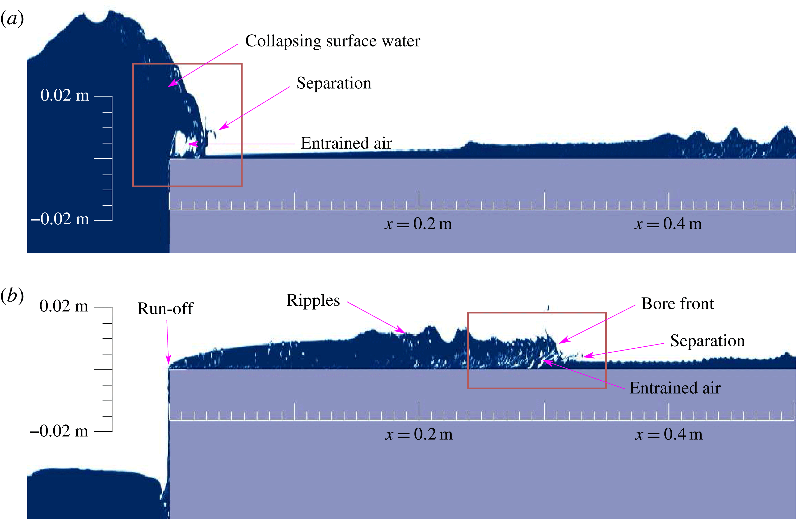
Snapshots of phase fraction produced by the CFD model with no-shear boundary conditions, produced by incident amplitude
 $a=20~\text{mm}$
, for: (a) an instant at which an incident wave forces overwash; and (b) an instant 0.4 s later, when a bore has formed in the overwash, and water washes off the step edge. Pure water (
 $\unicode[STIX]{x1D6FE}=1$
) is solid blue, pure air (
 $\unicode[STIX]{x1D6FE}=0$
) is solid white and the step is grey. The scale of the
 $z$
-axis is larger than the
 $x$
-axis scale by a factor 4 to emphasise overwash effects, and boxes highlight regions of greatest interest at the corresponding instants.

Figure 2 shows snapshots of the phase fraction,
 $\unicode[STIX]{x1D6FE}$
, for the test with the largest incident wave amplitude,
 $a=20~\text{mm}$
, i.e. the deepest overwash, and using the no-shear boundary conditions (similar behaviours occur for no-slip conditions). Figure 2(a) shows an instant during a phase when the incident wave forces overwash, with the box highlighting the interfacial region where a mass of water flows onto the step. As the incident wave hits the step the water above the step travels forwards, and the water just below the top of the step is pushed upwards, so that the top of the wave collapses onto the step. This creates wave overturning, similar to plunging breaker, just onto the step (as in Greco et al.
Reference Greco, Faltinsen and Landrini2005), and the overturning creates water separation. (Presumably, the separation is exaggerated by the neglect of surface tension, although noting that the separated water is indistinguishable from the water bulk at a 1 : 1 axes scale, not shown.) The roughness of the free surface in the interfacial region indicates prevalent wave breaking effects. These findings are qualitatively similar to those of Greco (Reference Greco2001) and Greco et al. (Reference Greco, Faltinsen and Landrini2005, Reference Greco, Colicchio and Faltinsen2007) from an experimental model of green water washing onto a ship deck, as described in § 1.
Figure 2(b) shows a snapshot
 $T/2=0.4~\text{s}$
later, when the overwashed water packet has travelled
 ${\sim}0.30~\text{m}$
along the step. The box highlights breaking around the bore front formed from the overwashed water, i.e. a fast-travelling sharp increase in depth (Chanson Reference Chanson2009). The water at the bore front is approximately 4 times deeper and 3.5 times faster than the water just ahead of it. The sharp increase in steepness at the bore causes the water near the upper surface to continually overturn the water below, creating the breaking, entrained air pockets, water separation and ripples seen around the bore. Breaking effects are largely confined to 0.2 m behind the bore front, and, although entrained air pockets are still present outside this region they are not as numerous or large as those near the bore front. The snapshot also shows water running off the step at
 $x=0$
. Its depth there is small relative to the overwash depth farther along the step and the depth of the water being forced onto the step 0.4 s earlier (figure 2
a), indicating the run-off volume is minor.
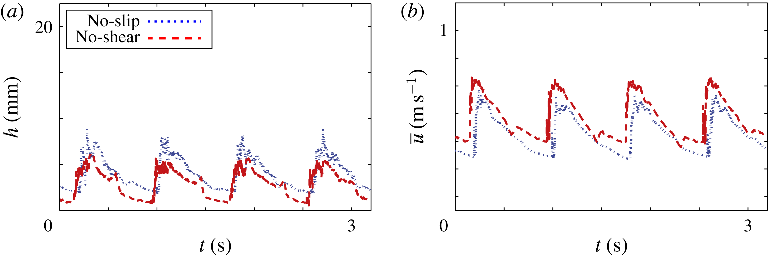
Figure 3 shows signals of the overwash depth and depth averaged horizontal velocity,
 $$\begin{eqnarray}h=\int _{0}^{\infty }\unicode[STIX]{x1D6FE}\,\text{d}z\quad \text{and}\quad \overline{u}=\frac{1}{h}\int _{0}^{\infty }\unicode[STIX]{x1D6FE}u\,\text{d}z,\text{respectively,}\end{eqnarray}$$
produced by the no-shear and no-slip models for the simulation with incident wave amplitude
 $a=15~\text{mm}$
. The signals are sampled at
 $x=0.2~\text{m}$
, by which point bores have developed, appearing in the signals as steep increases in both depth and velocity. The roughness of the signals, particularly at the bore fronts, indicate the breaking effects noted in figure 2(b). These behaviours and signal shapes are similar to those reported in the experiments of Buchner (Reference Buchner2002) for green water on a ship deck and Skene et al. (Reference Skene, Bennetts, Meylan and Toffoli2015) for overwash of a thin floating plate. The no-slip and no-shear boundary conditions produce similar depth and velocity signals, although the no-slip model consistently predicts deeper and slower overwash than the no-shear model. The systematic difference in depth and velocity is indicative of a boundary layer in the no-slip model.
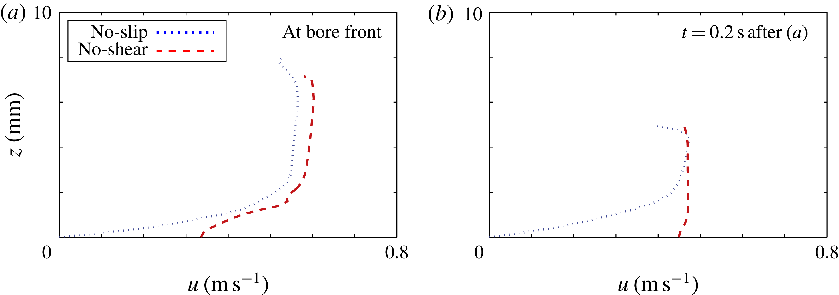
Figure 4 shows horizontal velocity profiles produced by the no-slip and no-shear models at
 $x=0.2~\text{m}$
for an incident wave amplitude
 $a=15~\text{mm}$
(as in figure 3). Figure 4(a) shows an instant when a bore front is at
 $x=0.2~\text{m}$
, and figure 4(b) is 0.2 s later, when the bore front has washed farther downstream from this location.
At the bore front, both models predict the water is faster at the surface than at the bed, indicating overturning will occur. Away form the bore front, the no-shear model predicts the velocity is approximately uniform through the water depth. The no-slip model predicts an approximately uniform velocity above
 ${\sim}2~\text{mm}$
depth only, below which the velocity rapidly tends to zero as the step surface is approached, confirming the presence of a boundary layer (Schlichting & Gersten Reference Schlichting and Gersten2016). The boundary layer was found to be approximately 2 mm deep for
 $x>0.1~\text{m}$
for all incident wave amplitudes tested, meaning it was relatively more significant for shallower overwash generated by smaller amplitude incident waves, and points farther along the step.
3 Mathematical model
Following Skene et al. (Reference Skene, Bennetts, Meylan and Toffoli2015), the water domain is split into two subdomains:
-
(i) the wave basin domain containing relatively deep water (
 $x<0$
); and
-
(ii) the overwash domain containing shallow water (
$x>0$
),


where the subdomains now stretch to infinity in the negative and positive
 $x$
-directions, respectively. The water in both subdomains is assumed to be irrotational, incompressible and inviscid.
CFD model predictions of overwash (a) depth and (b) depth averaged horizontal velocity, as functions of time, at
 $x=0.2~\text{m}$
for incident wave amplitude
 $a=15~\text{mm}$
, produced by no-shear (red dashed line) and no-slip (blue dotted) boundary conditions. The initial time,
 $t=0$
, is chosen as an arbitrary time once the overwash reaches periodic behaviour.

CFD model predictions of horizontal velocity,
 $u$
, as a function of height,
 $z$
, across the overwash depth at
 $x=0.2~\text{m}$
, for instants at which (a) a bore front is at the location, and (b) 0.2 s later, when the bore front has propagated downstream. As in figure 3, results are for incident wave amplitude
 $a=15~\text{mm}$
, and produced by no-shear (red dashed line) and no-slip (blue dotted) boundary conditions.

The water in Domain i (the basin) is modelled using linear potential-flow theory, on the basis that wave steepnesses are small, with the water velocity field defined as the gradient of a scalar velocity potential,
 $\unicode[STIX]{x1D719}(x,z,t)$
, satisfying Laplace’s equation throughout the linearised water domain,
 $x<0$
and
 $-H<z<0$
. Linearisation of the domain cuts off at the interface with the overwash domain (
 $x=0$
and
 $z>0$
), such that Domain i experiences no outward flux of water during the phase of overwash generation, and no inward flux of water during the run-off phase. The underlying assumption is that, as the depth of the basin is far greater than the overwash depth, the model of Domain i provides sufficiently accurate forcing for the overwash without incorporating the effects of the overwash.
Figure 5 shows a schematic of the linear potential-flow model in Domain i, including the standard boundary conditions. The boundary conditions are the linearised free surface condition (applied on the mean free surface,
 $z=0$
), no normal flow conditions applied on the basin floor (
 $z=-H$
) and the front surface of the step (
 $x=0$
and
 $-H<z<0$
), and the Sommerfeld radiation condition as
 $x\rightarrow -\infty$
(not shown). In the far field,
 $x\rightarrow -\infty$
, the motion consists of a rightward-propagating incident wave
 $$\begin{eqnarray}\unicode[STIX]{x1D719}_{I}(x,z)=\frac{ag}{\unicode[STIX]{x1D714}}\cos (\unicode[STIX]{x1D714}t-kx)\frac{\cosh \{k(z+H)\}}{\cosh (kH)},\end{eqnarray}$$
and a leftward-propagating reflected field. Solving the boundary-value problem for
 $\unicode[STIX]{x1D719}=\unicode[STIX]{x1D719}_{I}+\unicode[STIX]{x1D719}_{R}$
(e.g. using separation of variables), gives the reflected wave field as
 $\unicode[STIX]{x1D719}_{R}(x,t)=\unicode[STIX]{x1D719}_{I}(-x,z)$
, implying a standing wave field forms and indicating energy is conserved in the domain.
Schematic and governing equations for the linear potential-flow model of the basin water (not to scale).

The linear potential-flow predictions of the free surface elevation and the horizontal velocity at the free surface, respectively
 $$\begin{eqnarray}\unicode[STIX]{x1D702}(x,t)=\frac{-[\unicode[STIX]{x2202}_{t}\unicode[STIX]{x1D719}]_{z=0}}{g}\quad \text{and}\quad u_{0}(x,t)=[\unicode[STIX]{x2202}_{x}\unicode[STIX]{x1D719}]_{z=0},\end{eqnarray}$$
are used to force the overwash. These give
 $$\begin{eqnarray}\unicode[STIX]{x1D702}(x,t)=2a\sin (\unicode[STIX]{x1D714}t)\cos (kx)\quad \text{and}\quad u_{0}(x,t)=-2agk\unicode[STIX]{x1D714}^{-1}\cos (\unicode[STIX]{x1D714}t)\sin (kx).\end{eqnarray}$$
In Domain ii (the overwash), it is assumed that the water is shallow, such that horizontal length scales are much greater than vertical length scales, implying the vertical velocity is negligibly small when compared to horizontal velocity, i.e. the underlying assumption of shallow-water theory (Vreugdenhil Reference Vreugdenhil1994). The shallow-water assumption is motivated by observations of distinctive shallow-water properties, particularly bores, in laboratory experiments (e.g. Skene et al. Reference Skene, Bennetts, Meylan and Toffoli2015) and CFD simulations in § 2. Therefore, the overwash is modelled using the nonlinear shallow-water equations
 $$\begin{eqnarray}\displaystyle \unicode[STIX]{x2202}_{t}h+\unicode[STIX]{x2202}_{x}(h\overline{u}) & = & \displaystyle 0,\end{eqnarray}$$
 $$\begin{eqnarray}\displaystyle \text{and}\quad \unicode[STIX]{x2202}_{t}(h\overline{u})+\unicode[STIX]{x2202}_{x}\left(h\overline{u}^{2}+{\textstyle \frac{1}{2}}gh^{2}\right) & = & \displaystyle 0,\end{eqnarray}$$
 $h(x,t)$
is the water depth and
 $\overline{u}(x,t)$
is the depth averaged horizontal velocity. At the interface with Domain i (
 $x=0$
), if the free surface is above the step,
 $\unicode[STIX]{x1D702}(0,t)>0$
, the shallow-water depth is set to match the free surface elevation, and is set to zero otherwise. Similarly, if
 $\unicode[STIX]{x1D702}(0,t)>0$
the depth averaged horizontal velocity at the interface is set to match that in Domain i,
 $u_{0}(0,t)$
, and be zero otherwise. These conditions are defined at the lower limit of the boundary
 $x=0$
, as
 $$\begin{eqnarray}h(x=0^{-},t)=\max \{2a\sin (\unicode[STIX]{x1D714}t),0\}\quad \text{and}\quad \overline{u}(x=0^{-},t)=0,\end{eqnarray}$$
respectively, where the former condition uses
 $\unicode[STIX]{x1D702}(0,t)=2a\sin (\unicode[STIX]{x1D714}t)$
, and the latter uses
 $u_{0}(0,t)=0$
.
In the characteristic plane, boundary conditions (3.5) produce characteristics
 $X_{+}(x,t)$
that emanate from
 $x=0$
for
 $t>0$
, and enter Domain ii if
 $h(x=0^{-},t)>0$
. The associated slope,
 $\,\text{d}X_{+}/\,\text{d}t=\overline{u}+\sqrt{gh}$
, and Riemann invariant,
 $R_{+}=\overline{u}+2\sqrt{gh}$
, do not depend on the boundary values
 $h(0^{+},t)$
and
 $\overline{u}(0^{+},t)$
, thus forcing a hydraulic jump at
 $x=0$
for all
 $t$
, i.e. discontinuities
 $h(0^{+},t)\neq h(0^{-},t)$
and
 $\overline{u}(0^{+},t)\neq \overline{u}(0^{-},t)$
. The hydraulic jump results in water mass and energy propagating onto the step during the overwash generation phase,
 $\unicode[STIX]{x1D702}(0,t)>0$
, despite
 $\overline{u}(x=0^{-},t)=0$
being prescribed, and mass and energy propagating off the step during the run-off phase,
 $\unicode[STIX]{x1D702}(0,t)\leqslant 0$
.
During the overwash generation phase with
 $\unicode[STIX]{x1D702}(0,t)$
increasing, the shallow-water Froude number,
 $Fr=\overline{u}/\sqrt{gh}$
, passes through unity a short distance along the step (approximately
 $0<x<a/10$
), meaning the flow transitions from sub- to super-critical. This generates one shock (i.e. a travelling hydraulic jump) per wave period in the overwash (Vreugdenhil Reference Vreugdenhil1994; Chanson Reference Chanson2009), which are regarded as bores in the water wave context. The shocks/bores dissipate energy as they propagate along the step (see, e.g. Billingham & King Reference Billingham and King2000, § 8.1).
Following Skene et al. (Reference Skene, Bennetts, Meylan and Toffoli2015), a shock-capturing numerical scheme is used to solve the shallow-water problem (3.4)–(3.5). The scheme consists of Kurganov & Tadmor’s (Reference Kurganov and Tadmor2000) finite-volume method in space and the total variation diminishing second-order Runge–Kutta method in time (Gottlieb & Shu Reference Gottlieb and Shu1998). It captures shocks without creating unnatural numerical oscillations that force the depth to become negative. Boundary conditions (3.5) are applied at a ghost volume centred at
 $x=-\unicode[STIX]{x0394}x$
, where
 $\unicode[STIX]{x0394}x$
is the volume width used in the numerical scheme, such that the hydraulic jump occurs over the
 $x=0$
volume. Therefore, mathematical model predictions of overwash properties at the interface,
 $x=0^{+}$
, presented in § 4, are taken from the
 $x=\unicode[STIX]{x0394}x$
volume. Convergence with respect to
 $\unicode[STIX]{x0394}x$
was analysed for
 $0.0001<a<0.1~\text{m}$
, and for
 $\unicode[STIX]{x0394}x\approx 0.003\sqrt{a}$
it was found that
 $h$
and
 $\overline{u}$
were within 0.8 % of the values given by cell width of
 $0.01\unicode[STIX]{x0394}x$
. For simplicity, and to sufficiently resolve the bore fronts, all results are presented using
 $\unicode[STIX]{x0394}x=0.25~\text{mm}\ll 0.003\sqrt{a}$
, for all incident wave amplitudes tested. A numerical radiation condition for
 $x\gg 0$
is set as
 $\overline{u}(R,t)=h(R,t)=0$
, where
 $R=2~\text{m}$
(approximately four times the distance between adjacent bore fronts) was found to be suitably large that the overwash depth and depth averaged velocity for
 $0<x<0.5~\text{m}$
are insensitive to increasing
 $R$
.
Simulations were run up to
 $t=15~\text{s}$
(noting that the mathematical model does not require a time interval for waves to build up and reach the step), using the same incident wave amplitude–period combinations as the CFD model in § 2. As in the CFD simulations, periodic overwash motions were attained after
 ${\sim}5$
periods of the forcing waves. Each simulation required only
 ${\sim}0.2~\text{h}$
on a single core, representing a 600-fold speed up in comparison to the CFD models (which were run on a 96 core cluster).
4 Model comparisons
4.1 Overwash depth and horizontal velocity
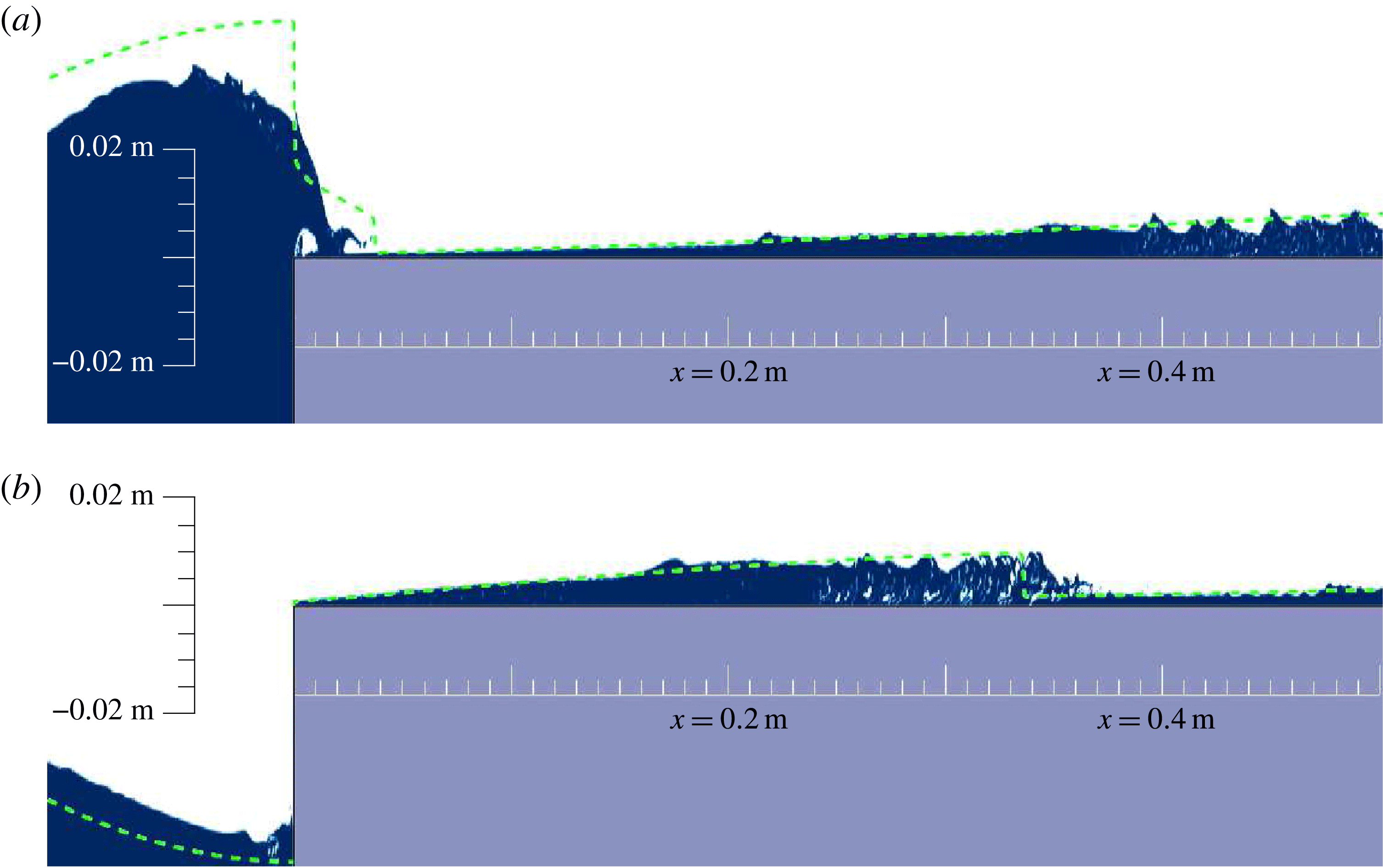
Figure 6 shows snapshots of the phase fraction produced by the no-shear CFD model, as in figure 2 but for the mid-range amplitude
 $a=15~\text{mm}$
, and with corresponding mathematical model predictions of the free surface (and hence the water depth) superimposed. Time offsets are applied such that the maximum wave elevation at
 $x=0$
is aligned between the models. The comparisons shown are typical of all incident wave conditions tested.
As in figure 2 but for
 $a=15~\text{mm}$
, with the mathematical model free surface overlaid (dashed green), and with (b) showing an instant 0.5 s after (a).

As in figure 2(a), figure 6(a) shows a snapshot for an instant at which an incident wave forces overwash. The mathematical model prediction of the free surface in the interfacial region is markedly different from the CFD model, initially underpredicting the free surface in the interval where an air cavity is present in the CFD model, and subsequently overpredicting the free surface in the interval where the overturning free surface passes onto the step in the CFD model. Beyond this interfacial region, the mathematical model predicts a near identical free surface profile (overwash depth) to the CFD model, but does not capture the ripples present in the CFD model for
 $x>0.4~\text{m}$
.
Figure 6(b) shows a snapshot 0.5 s later, at which point the overwash has propagated along the step. Both models predict that a bore develops, and the locations of the bore fronts are
 ${<}15~\text{mm}$
apart after washing 350 mm downstream, noting that the exact location of the bore front is ill defined in the CFD simulation because the jump in depth is not instantaneous as in the shallow-water model. Moreover, the bore heights, and more generally, the overwash depth profiles, display pleasing agreement (notwithstanding the breaking effects present around the bore in the CFD simulation), indicating the mathematical model accurately predicts overwash beyond the interfacial region, despite neglecting air cavitations and wave breaking effects.
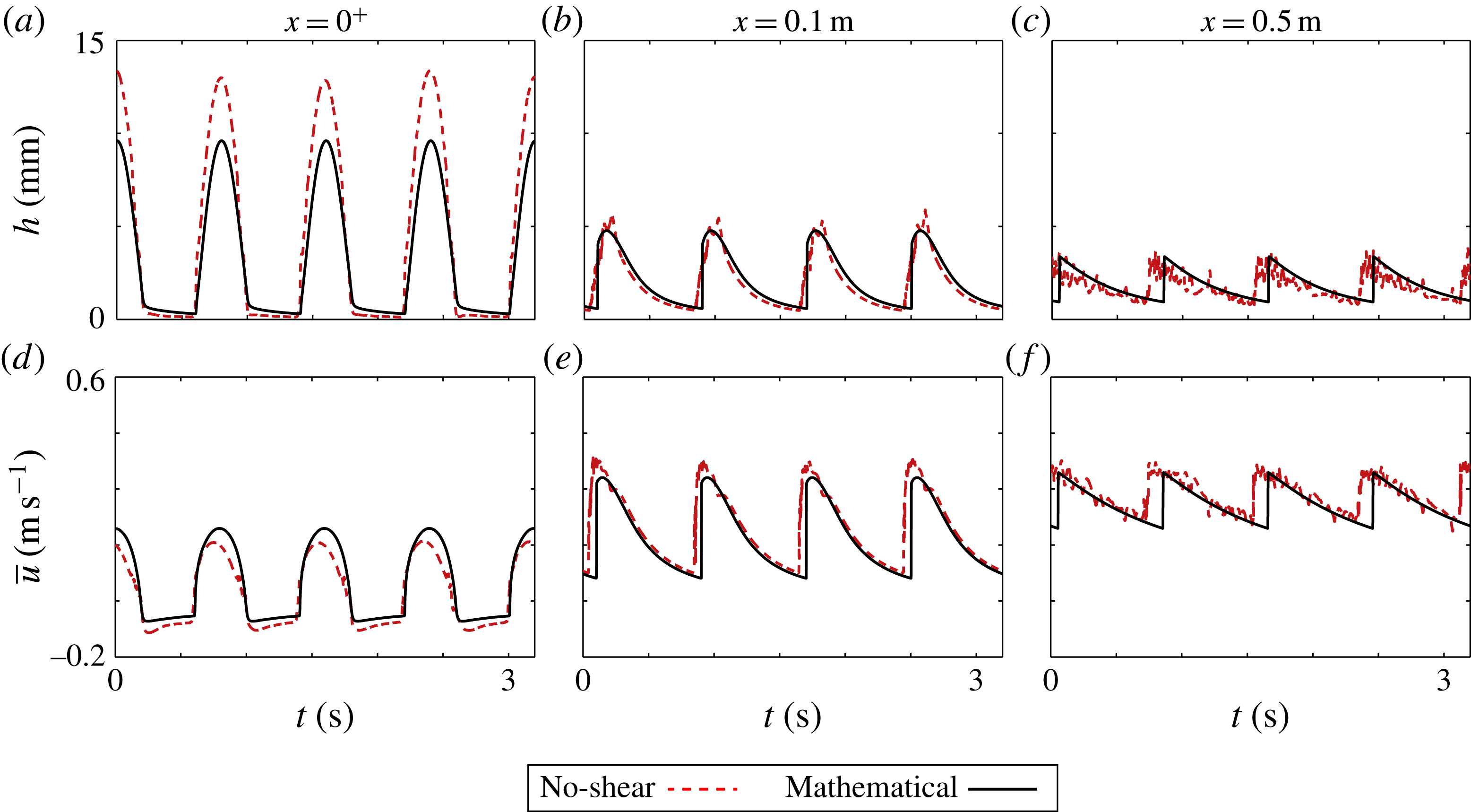
Depth versus time (a–c) and depth averaged velocity versus time (d–f) predictions given by mathematical model (solid black curves) and no-shear CFD model (broken red), for incident wave amplitude
 $a=10~\text{mm}$
, and sampled at
 $x=0^{+}$
(a,d), 0.1 m (b,e), and 0.5 m (c,f) along the step.

Figure 7 shows depth and depth averaged horizontal velocity signals, given by the mathematical model (solid black) and no-shear CFD model (dashed red), sampled at
 $x=0^{+}$
, 0.1 and 0.5 m. Results are provided for the incident wave amplitude
 $a=10~\text{mm}$
, which is representative of all incident waves tested. The first location,
 $x=0^{+}$
, compares the models at the interface between the basin and overwash. The depth signals (figure 7
a) are composed of approximately symmetric peaks, corresponding to the wave surface in the basin rising above the step, separated by intervals of approximately zero depth, when the surface dips below the step. As indicated in figure 6(a), the mathematical model predicts smaller depth peaks than the no-shear CFD model, with
 ${\sim}3~\text{mm}$
differences at the peaks, and noting that the depth integration in (2.3) eliminates the air cavity in the CFD model. The models predict similar velocity signals at the interface (figure 7
b), although the mathematical model predicts slightly larger peaks and shallower troughs, and the CFD model predicts positively skewed peaks. The run-off phase (negative velocity) occurs for approximately half of the duration of the overwash cycle. During this phase, the mathematical no-shear CFD models predict similar depths and velocities, indicating that the models predict a similar amount of run-off.
The second location,
 $x=0.1~\text{m}$
, is where bores have just formed (as in figure 3, the bores manifest in the signals as sharp, concomitant increases in depth and velocity). The models agree closely for both depth and velocity signals, in terms of overall shape, phase, peaks and troughs. For the depth signals, the most notable difference is due to coarseness around the bore peaks predicted by the no-shear CFD model. For the velocities, the signals given by the models have small phase differences of
 ${\sim}0.05~\text{s}$
, which is 6 % of the wave period only, and the velocity predicted by the CFD model is consistently
 $0.04~\text{m}~\text{s}^{-1}$
greater than predicted by the mathematical model.
The final location,
 $x=0.5~\text{m}$
, is a point at which the no-shear CFD model predicts air entrainment and breaking effects are prevalent in the bores (as indicated in figure 6
b). The shapes of the depth and velocity signals are similar to the corresponding signals at
 $x=0.1~\text{m}$
, with bores still pronounced, but with reduced peaks for the depth and velocity signals. The ongoing breaking effects in the CFD simulations create a high degree of roughness in the corresponding signals. Overall agreement between the models remains strong, although the phase shift in the depth and velocity signals increases to 0.1 s. This phase difference is a symptom of the mathematical model predicting slightly slower bores than the CFD model.
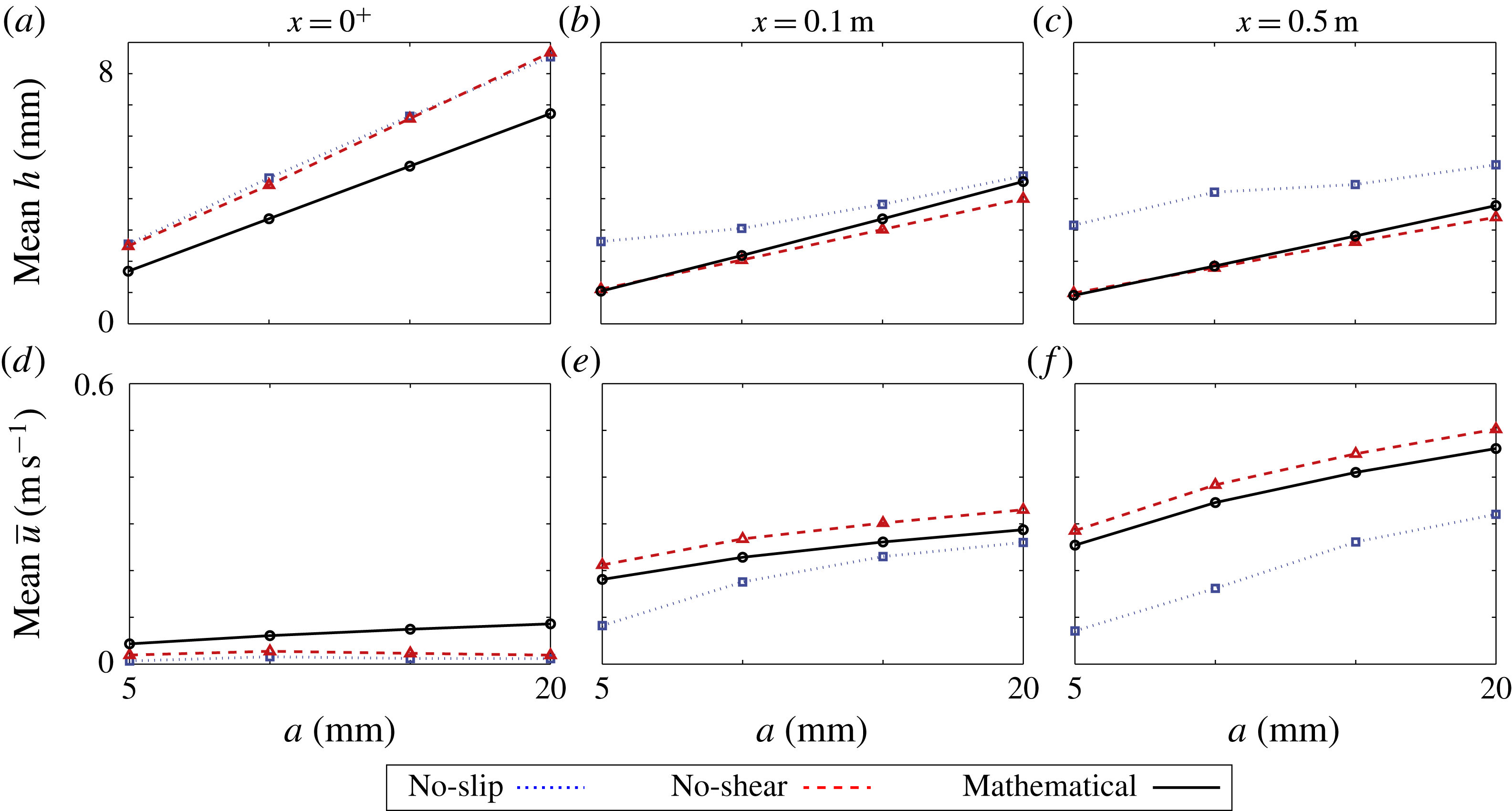
Mean depth versus amplitude (a–c) and mean depth averaged horizontal velocity versus amplitude (d–f), predicted by mathematical model (solid black curves and circles), no-shear CFD model (dashed red and triangles) and no-slip CFD model (dotted blue and squares), sampled at
 $x=0^{+}$
(a,c), 0.1 m (b,e), and 0.5 m (c,f) along the step.

Figure 8 shows mean values of overwash depth (a–c) and depth averaged velocity (d–f) over four wave periods, as a function of incident wave amplitude, and for the three locations used in figure 7 (
 $x=0^{+}$
, 0.1, and 0.5 m). Results are given for the mathematical model (solid black lines and circles), and the CFD model with no-shear boundary conditions (dashed red lines and triangles) and no-slip conditions (dotted blue lines and squares).
In all cases, the mean depth increases as the incident wave amplitude increases, as expected, and generally decreases with distance along the step, as indicated in figure 7. The CFD models agree almost exactly at the basin–overwash interface (
 $x=0^{+}$
, figure 8
a), indicating the boundary layer in the no-slip CFD model does not affect the overwash forcing, and the depths increase in proportion to the incident amplitude. As shown in figures 6 and 7, at the interface the mathematical model is shallower than the CFD models, with the difference in depth increasing as wave amplitude increases, although it also predicts the depth increases in proportion to the incident amplitude. At the two points farther along the step,
 $x=0.1~\text{m}$
and
 $x=0.5~\text{m}$
(figure 8
b,c), the mathematical model and no-shear CFD model predict similar depths, with both predicting the depths increase in proportion to the incident amplitude. The mathematical model predicts slightly greater depths, with the difference decreasing farther along the step and increasing as incident amplitude increases. For example, at
 $x=0.1~\text{m}$
the models differ by
 ${<}0.4~\text{mm}$
(11 %) for
 $a\leqslant 15~\text{mm}$
, and by 1.5 mm (14 %) for
 $a=20~\text{mm}$
. The no-slip CFD model predicts notably deeper overwash at these locations due to the boundary layer discussed in § 2.2, and does not predict that the depth increases in proportion to the incident amplitude.
The mean depth averaged horizontal velocity of the overwash tends to increase as the incident wave amplitude increases and with distance along the step. Similar to the mean depths, at the interface,
 $x=0^{+}$
(figure 8
d), the velocities predicted by the CFD models agree (differences
 ${<}0.01~\text{m}~\text{s}^{-1}$
). The mathematical and the no-shear CFD models agree farther along the step (figure 8
e,f), although the no-shear CFD model systematically predicts
 ${\sim}0.04~\text{m}~\text{s}^{-1}$
greater velocities for all amplitudes and locations (corresponding to a relative difference between 11–15 % at
 $x=0.1$
and 8–10 % at
 $x=0.5~\text{m}$
). At the interface, the CFD models predict positive mean velocities but only very small values, whereas the mathematical model predicts positive values up to a factor of eight greater than the CFD models. Farther along the step, the no-slip CFD model predicts slower overwash than the other models, again due to the presence of a boundary layer.
4.2 Overwash mass and energy fluxes
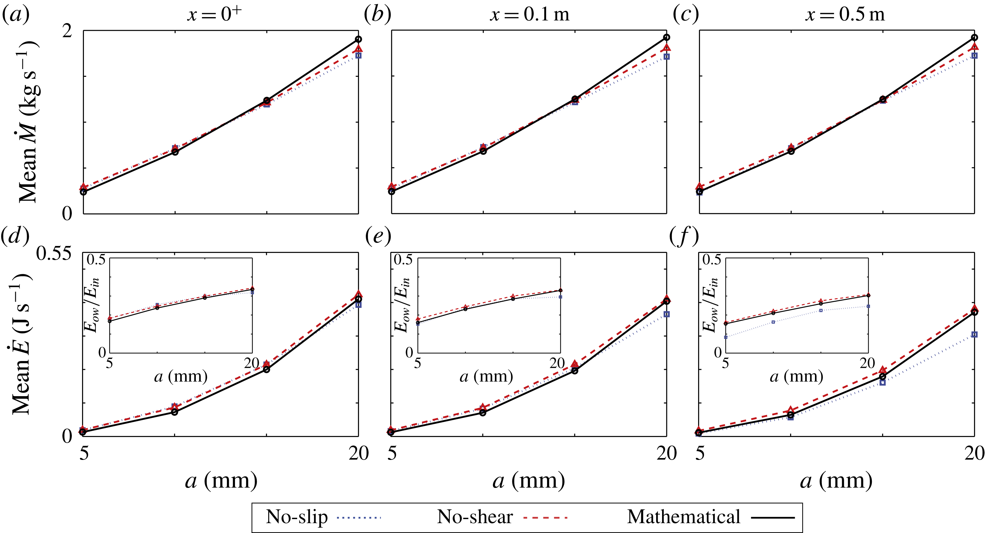
As in figure 8 but for the mean mass flux and mean energy flux. Insets in (d–f) show the mean mass flux as a portion of the incident wave energy flux.

Figure 9 is similar to figure 8, but for the mean mass flux (a–c) and mean energy flux (d–f). The mass flux (through a vertical cross-section),
 ${\dot{M}}$
, is given by
 $$\begin{eqnarray}{\dot{M}}=\unicode[STIX]{x1D70C}_{w}\overline{u}h\quad \text{and}\quad {\dot{M}}=\int _{0}^{\infty }\unicode[STIX]{x1D70C}_{w}u\unicode[STIX]{x1D6FE}\,\text{d}z,\end{eqnarray}$$
for the mathematical and CFD models, respectively. The energy flux (also through a vertical cross-section),
 ${\dot{E}}$
, is given as the flux of kinetic and potential energies plus the work done by pressure over the cross-section. It is
 $$\begin{eqnarray}{\dot{E}}=\frac{1}{2}\unicode[STIX]{x1D70C}_{w}\overline{u}^{3}h+\unicode[STIX]{x1D70C}_{w}g\overline{u}h^{2}\quad \text{and}\quad {\dot{E}}=\int _{0}^{\infty }\unicode[STIX]{x1D70C}_{w}\left(\frac{1}{2}\boldsymbol{u}\boldsymbol{\cdot }\boldsymbol{u}u\unicode[STIX]{x1D6FE}+gzu\unicode[STIX]{x1D6FE}\right)+pu\unicode[STIX]{x1D6FE}\,\text{d}z,\end{eqnarray}$$
for the mathematical and CFD models, respectively, where the atmospheric pressure in the surrounding air is normalised to
 $p_{atm}=0$
, and noting that the second component of (4.2) reduces to the first component as pressure becomes hydrostatic under the shallow-water assumption (Vreugdenhil Reference Vreugdenhil1994). The fluxes are averaged over four wave periods. The insets in figure (d–f) show the energy flux in the overwash through a vertical cross-section averaged over a wave period,
 $E_{ow}$
, as a proportion of the time averaged energy flux of the incident wave through a vertical cross-section,
 $E_{in}$
. For the mathematical model
 $$\begin{eqnarray}E_{in}=\frac{\unicode[STIX]{x1D70C}_{w}\unicode[STIX]{x1D714}ga^{2}}{4k}\left(1+\frac{2kH}{\sinh (2kH)}\right),\end{eqnarray}$$
and this expression is also used for the CFD models, as higher-order effects have a negligible impact on the mean energy flux (Whitham Reference Whitham1962).
The mass fluxes (figure 9
a–c) increase in a weakly superlinear trend, with respect to increasing incident wave amplitude. The mass fluxes are independent of the measurement location, which is a consequence of the models being based on conservation of mass. The mathematical and CFD models closely agree, particularly for mid-range amplitudes
 $a=10$
and 15 mm, where the maximum difference is only
 $0.05~\text{kg}~\text{s}^{-1}$
(a relative difference of
 ${\sim}5\,\%$
), and least well for the largest incident amplitude
 $a=20~\text{mm}$
, where the mathematical model predicts a flux
 $0.11~\text{kg}~\text{s}^{-1}$
greater than the no-shear CFD model, and
 $0.17~\text{kg}~\text{s}^{-1}$
greater than the no-slip CFD model. The relative difference between the mathematical and no-shear model for
 $a=20~\text{mm}$
remains
 ${\sim}5\,\%$
, but the relative difference between mathematical and no-slip model increases to
 ${\sim}9\,\%$
.
The energy fluxes (figure 9
d–f) display a stronger superlinear increase with respect to increasing incident wave amplitude than the mass fluxes, and decrease with distance along the step. At the interface,
 $x=0^{+}$
, the models closely agree, with differences only
 ${<}0.02~\text{J}~\text{s}^{-1}$
. This level of agreement is maintained at the point where bores have just developed,
 $x=0.1~\text{m}$
, except for the largest incident amplitude, where the no-slip CFD model predicts an energy flux
 ${\sim}0.04~\text{J}~\text{s}^{-1}$
less than the other models. At the farthest location along the step,
 $x=0.5~\text{m}$
, the differences between the mathematical and no-shear CFD models are still
 ${<}0.02~\text{J}~\text{s}^{-1}$
, but the no-slip CFD model consistently predicts the smallest energy fluxes, with differences increasing as the incident amplitude increases, up to
 $0.07~\text{J}~\text{s}^{-1}$
(
 ${\sim}23\,\%$
) for the largest incident amplitude.
The decreases in energy flux along the step (from
 $x=0$
to 0.5 m) are 9.5–12 % for both the mathematical and no-shear CFD models. This is an energy flux reduction of approximately
 $0.003~\text{J}~\text{s}^{-1}~\text{m}^{-1}$
and
 $0.078~\text{J}~\text{s}^{-1}~\text{m}^{-1}$
over the 0.5 m for the lowest and highest incident amplitude, respectively. Breaking effects around the bores are the primary source of energy dissipation in the no-shear CFD model, whereas energy dissipation in the mathematical model is a consequence of the discontinuity over the bore. The agreement in energy flux indicates that the energy losses due to the highly complicated breaking bores in the no-shear CFD model are similar to those predicted by the bores in the shallow-water model.
The no-slip CFD model predicts significantly larger decreases in energy flux along the step, due to additional viscous forces in the boundary layer (Schlichting & Gersten Reference Schlichting and Gersten2016), with a decrease of 54 % for the smallest incident amplitude, and 24 % for the largest amplitude. This corresponds to a much larger average energy flux decrease of
 $0.020~\text{J}~\text{s}^{-1}~\text{m}^{-1}$
and
 $0.177~\text{J}~\text{s}^{-1}~\text{m}^{-1}$
over the 0.5 m distance, for the lowest and highest incident amplitudes, respectively.
Figure 9(d–f) insets show the models predict 15–35 % of the incident wave energy enters the overwash, and that a greater portion of the incident wave energy enters the overwash as the incident amplitude increases (in a weakly sublinear trend). At
 $x=0^{+}$
, the models differ by less than 3 %. Farther along the step, at
 $x=0.1$
and 0.5 m, the mathematical and no-shear CFD models retain this agreement, and predict decreases in energy flux
 ${<}4\,\%$
of the incident energy flux from
 $x=0^{+}$
to
 $x=0.5~\text{m}$
, for all amplitudes tested. The no-slip CFD model predicts a larger decrease in energy flux, ranging from 13 % of the incident energy flux for
 $a=5~\text{mm}$
, to 8 % for
 $a=20~\text{mm}$
.
4.3 Shallow-water transition
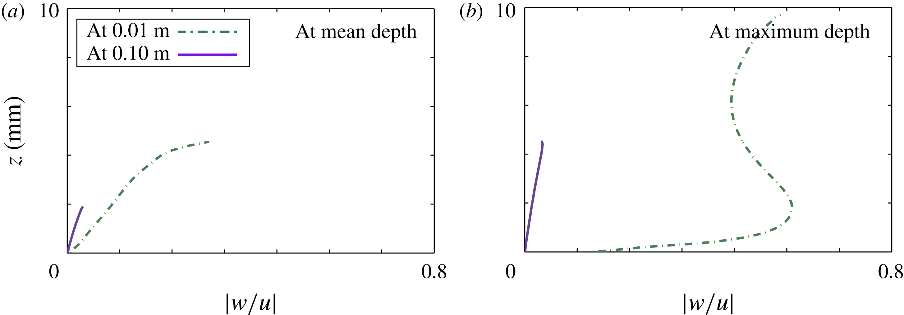
Magnitude of vertical velocity divided by horizontal velocity as functions of height,
 $z$
, by no-shear CFD model, sampled at
 $x=0.01~\text{m}$
(broken green curves) and
 $x=0.1~\text{m}$
(solid purple curves) produced by incident amplitude
 $a=10~\text{mm}$
, for instants of time when overwash at the respective locations are: (a) at their mean depths; and (b) at their maximum depths.

Figure 10 shows no-shear CFD model predictions of
 $|w/u|$
(i.e. the magnitude of the vertical velocity divided by the horizontal velocity), with respect to height
 $z$
, for instants of time when the overwash is at its mean depth (a) and maximum depth (b), at
 $x=0.01~\text{m}$
and 0.1 m, noting that bores develop for
 $0.02<x<0.1~\text{m}$
(in all cases tested). Therefore, the location
 $x=0.01~\text{m}$
represents behaviours in the transition onto the step, and
 $x=0.1~\text{m}$
represents locations where bores have just developed. Corresponding profiles given by the no-slip CFD model (not presented) are similar, although the velocity ratio is marginally smaller for
 $z$
less than approximately 1.5 mm.
At
 $x=0.1~\text{m}$
, the vertical velocity is always at least an order of magnitude less than the horizontal velocity in both instances, with
 $|w/u|<0.033$
, but generally much less. In contrast, at
 $x=0.01~\text{m}$
, the vertical velocity is frequently the same order of magnitude as the horizontal velocity, particularly when the overwash is at its maximum depth, where
 $|w/u|=0.6$
–0.7 through most of the water depth. Therefore, the no-shear CFD model predicts the overwash transitions to being shallow – in the sense of the underlying assumption of shallow-water theory that the vertical velocity is much less than the horizontal velocity (Vreugdenhil Reference Vreugdenhil1994) – in the interval
 $0<x\leqslant x_{trans}<0.1~\text{m}$
. This indicates the shallow-water model of the overwash is valid for
 $x\geqslant x_{trans}$
, partially explaining the differences between the overwash heights and velocities predicted by the mathematical model and the CFD models at the interface (
 $x=0^{+}$
), and the close agreement between the mathematical model and no-shear CFD model for
 $x\geqslant 0.1~\text{m}$
, as shown in figures 6 and 7. The transition to agreement in terms of height and velocity implies underlying agreement between the models, and figure 9 provides evidence that it is agreement in terms of mass and energy fluxes that guides the transition, noting that both models are based on conservation of mass and momentum (closely related to energy).
Defining the water to be shallow when the vertical velocity is an order of magnitude less than the horizontal velocity for all
 $t$
, in all cases tested
 $x_{trans}<0.05~\text{m}$
. Therefore, the transition distance,
 $x_{trans}$
, is much less than (by at least an one order of magnitude) the distance between bore fronts (
 ${\sim}0.5~\text{m}$
) and the incident wavelength (
 $\unicode[STIX]{x1D706}=1.0~\text{m}$
), i.e. the horizontal length scales in the overwash and basin, respectively. Additionally, it was found that the value of
 $x_{trans}$
increases as the incident wave amplitude increases (not shown), partially explaining the better agreement between depths and velocities predicted by the mathematical and no-shear models at
 $x=0.1~\text{m}$
in figure 8(b,e) for smaller incident amplitudes. Moreover, the CFD model (with no-shear or no-slip conditions) predicts
 $|w/u|$
becomes smaller the farther the overwash propagates along the step, explaining the improved agreement between no-shear and mathematical model from
 $x=0.1~\text{m}$
(figure 8
b,e) to
 $x=0.5~\text{m}$
(figure 8
c,f).
5 Conclusions
Overwash of a step by small steepness, regular incident waves has been analysed using a CFD model, based on the two-phase, incompressible Navier–Stokes equations, and a mathematical model, based on combined linear potential-flow and nonlinear shallow-water theories. The CFD model was shown to capture overturning, vortices, and air entrainment at the step front where the overwash is generated, as well as breaking in the bores along the step, but at a heavy computational expense (120 h on 96 cores per 30 s of simulation). The mathematical model neglects the complex dynamics at the step front where the overwash is generated, but runs significantly faster than the CFD model and on a single core only (0.2 h for 15 s simulation time).
The main findings of the investigation are:
-
(i) The models predict the proportion of incident wave energy forced into the overwash ranges from 16 % for the smallest incident wave amplitude tested, to 35 % for the largest amplitude.
-
(ii) No-slip boundary conditions on the step surfaces create an
${\sim}2~\text{mm}$
thick boundary layer (consistent for all incident wave amplitudes tested at period
$T=0.8~\text{s}$
), making the overwash deeper and slower than in simulations where no-shear boundary conditions were applied. -
(iii) The mathematical model predicts shallower and faster overwash than the CFD models directly above the front of the step, but near identical depths and depth averaged horizontal velocities to the CFD model with no-shear boundary conditions farther along the step where bores have developed.
-
(iv) The mathematical and no-shear CFD models predict almost identical mean mass and energy fluxes at the step edge and along the step. This provides an explanation of why the models agree in terms of depths and velocities once the CFD model transitions to a shallow-water flow despite the significant differences where the overwash is generated. The no-slip CFD model predicts smaller energy fluxes as the overwash propagates along the step, which was attributed to energy dissipation in the boundary layer.


This investigation indicates that a low-cost mathematical model, based on linear potential-flow theory to model overwash forcing and shallow-water theory to model the overwash itself, is viable to model the overwash phenomenon, although extensions of the shallow-water theory are necessary to model boundary-layer effects in the overwash. It follows that the mathematical model overpredictions of overwash depths at the centre of a thin floating plate found by Skene et al. (Reference Skene, Bennetts, Meylan and Toffoli2015) are most likely due to collisions between bores from the leading and training ends of the plate. A numerical approach would be necessary to model this phenomenon, although it potentially has negligible effect on the mass and energy being forced into the overwash, which is arguably the most important quantity in the context of predicting the effect of overwash on the surrounding wave field.
Acknowledgements
An Australian Postgraduate Award funds a PhD scholarship for DMS. The Australian Antarctic Science Program funds LGB and DMS (project 4123). The U.S. Office of Naval Research supports MHM (award number N00014-15-1-2611), and M.W. and K.J.M. This work used the Extreme Science and Engineering Discovery Environment (XSEDE), which is supported by National Science Foundation grant no. ACI-1548562. This research was supported in part through computational resources and services provided by Advanced Research Computing at the University of Michigan, Ann Arbor.