Introduction
The evolution of the fifth generation (5G) mobile communication technology escalates the demands for spectrum resources and data transmission rates. Multiple-input multiple-output (MIMO) technology is central to meeting this demand by increasing channel capacity, which is typically achieved by deploying more antenna elements within a limited space. However, this dense integration inevitably intensifies mutual coupling between elements, degrading system performance. Consequently, achieving effective decoupling without sacrificing compactness constitutes a fundamental challenge in MIMO antenna design [Reference Yousfi, Abdalmalak, Lamkaddem, Barrera, Biscontini and Vargas1, Reference Yousfi, Lamkaddem, Abdalmalak and Vargas2, Reference Lin and Chen27].
In recent years, various methods have been proposed to mitigate the mutual coupling between MIMO antenna elements. Representative approaches include coupling suppression through structural modifications such as defected ground structures (DGSs) [Reference Elalaouy, Ghzaoui and Foshi3], metamaterial configurations [Reference Hasan, Islam, Alam, Alzamil and Soliman4], and coupling cancellation utilizing neutralization lines [Reference Wu, Wang and Chen5], or parasitic decoupling structures between radiating elements [Reference Dkiouak, Rahmani, Ouahabi, Zakriti, Baghouri and El Mamouni6, Reference Ayinala and Sahu7]. While effective, these approaches often increase design complexity and footprint. To address spatial constraints, self-decoupling techniques have emerged as a promising alternative [Reference Geoffrey and Krishnan8–Reference Hung, Hong, Nguyen, Tran-Viet and Park12]. For example, a differential feeding technique enables over 40 dB self-decoupling [Reference Geoffrey and Krishnan8]. Hussain et al. achieve over 30 dB isolation through polarization diversity [Reference Hussain, Awan, Alzaidi and Elkamchouchi9]. A key self-decoupling strategy exploits inherent modal properties. For example, characteristic mode analysis has been applied to guide structural evolution, achieving isolation greater than 24 dB [Reference Modak, Lokam and Farooq10]. Alternatively, exciting specific orthogonal modes (TM10 and TM02) in excited and non-excited elements has also proven effective [Reference Phuong, Thang and Thanh11, Reference Hung, Hong, Nguyen, Tran-Viet and Park12]. Despite these significant advancements in isolation, persistent challenges such as narrow bandwidth and insufficient compactness remain critical limitations for further investigation.
To overcome the narrowband limitations of patch antennas, researchers have proposed metasurface (MS)-integrated MIMO configurations. These designs utilize the unique electromagnetic properties of MSs to broaden bandwidth and enhance isolation. A common approach is to place an MS decoupling array above the radiating patches, which improves isolation but often requires an air gap that increases the profile [Reference Raza, Zhang and Yan13–Reference Tariq, Naqvi, Hussain and Amin16, Reference Angadi, Sharma, Raghava and Sabapathy25, Reference Angadi, Sharma, Raghava and Sabapathy26]. To achieve a lower profile, MSs composed of periodic split-ring resonators [Reference Wang, Li and Yin14] or square cells [Reference Hussain, Jeong, Abbas and Kim17] have been integrated around patch antennas, achieving isolations greater than 25 and 30 dB respectively. Beyond the traditional periodic analysis method MS design, research on self-decoupling MS antennas based on characteristic modes analysis (CMA) has also emerged. For example, CMA has been used to achieve self-decoupling via mode separation and higher-order mode suppression [Reference Gerami and Kazemi18]. Ding et al. excited four orthogonal radiation modes through CMA, realizing over 20 dB isolation [Reference Ding, Liu, Ran, Wu, Liu and Fu19]. Zeng et al. introduced a set of metal vias into a densely arranged MS MIMO structure to control the mode electric fields of non-excited elements, thereby achieving self-decoupling through electric field cancellation [Reference Zeng, Chen and Liang20]. Li et al. applied CMA and shaping techniques to suppress coupling modes for self-decoupling, achieving an isolation of up to 45 dB [Reference Li, Nan, Xu, Chen and Feng23]. While these MS-based methods have yielded significant decoupling effects, their overall footprints and profiles still require further optimization.
In this paper, a compact MS antenna with flat gain is proposed based on CMA. The antenna comprises an intimately integrated MS layer and a rectangular patch antenna, forming a low-profile structure with optimized compactness. Horizontal slots in the central MS units separate and reconfigure the dominant mode. A coaxial feed then simultaneously excites the TM10 modes of both the patch and the MS, yielding a −10 dB impedance bandwidth from 3.45 to 4.5 GHz, a peak gain of 6.8 dBi, and an in-band gain fluctuation of less than 1.9 dB. In addition, a dual-port self-decoupled MIMO antenna is constructed by orthogonally arranging two antenna elements. Measurements demonstrate an operating band of 3.44–4.39 GHz, featuring over 23.6 dB isolation, a peak gain of 4.7 dBi, and gain fluctuation below 0.8 dB. These results confirm the antenna’s compact structure, excellent diversity, and stable radiation, validating its suitability for compact 5G NR (New Radio) applications.
Single-port MS antenna
Antenna structure
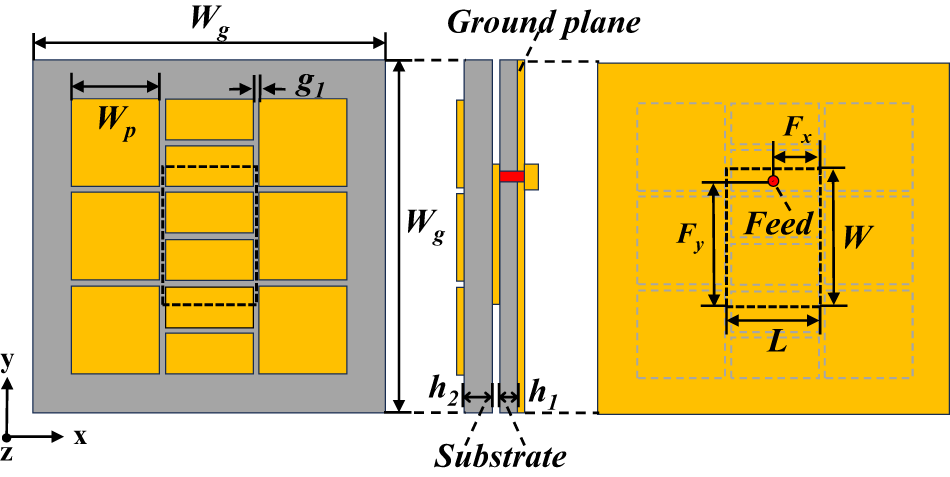
The structure of the proposed single-port MS antenna is shown in Fig. 1. The antenna comprises a top MS layer, a rectangular patch layer, and a bottom ground plane. The MS consists of 3 × 3 square patch cells, with a slot etched at the center of each cell in the middle column. Both dielectric substrates are FR4 material (relative dielectric constant ε r of 4.4 and loss angle tangent of 0.02). The rectangular patch is fed by a 50 Ω coaxial probe. The optimized geometrical parameters of the antenna are listed in Table 1.
Geometry of the single-port MS MIMO antenna.

Figure 1 Long description
The diagram illustrates the geometry of a single-port MS MIMO antenna through three distinct views. On the left, a top view displays a grid of nine square patch cells arranged in a three by three configuration. Each cell in the middle column has a slot etched at its center. The dimensions are labeled with W subscript g for the width of the ground plane, W subscript p for the width of the patch and g subscript l for the gap between patches. The middle view is a side profile showing the layered structure of the antenna, including the ground plane and substrate, with dimensions h subscript 1 and h subscript 2 indicating the thickness of the layers. The right view provides a detailed layout of a single patch, highlighting the feed point marked in red. Dimensions are labeled as F subscript x and F subscript y for the feed position and W and L for the width and length of the patch. The substrate is indicated below the layers and the coordinate axes x, y and z are shown for reference.
The dimension parameters of antenna

Table 1 Long description
The table lists physical dimension parameters for an antenna, with all values given in millimeters. The largest dimension is Lg at 75 mm, followed by Wg at 40 mm. Mid-sized dimensions include W at 16 mm, Wd at 14.5 mm, Fy at 14.8 mm, and Lp at 11.65 mm, with L and Lp close in size. Smaller features include Wp at 10 mm and Fx at 5.5 mm. The smallest values are the gaps g1 at 0.7 mm and g2 at 4.3 mm, plus heights h1 at 1.8 mm and h2 at 3 mm. One parameter entry is blank in the final row, so the dataset appears incomplete for that position.
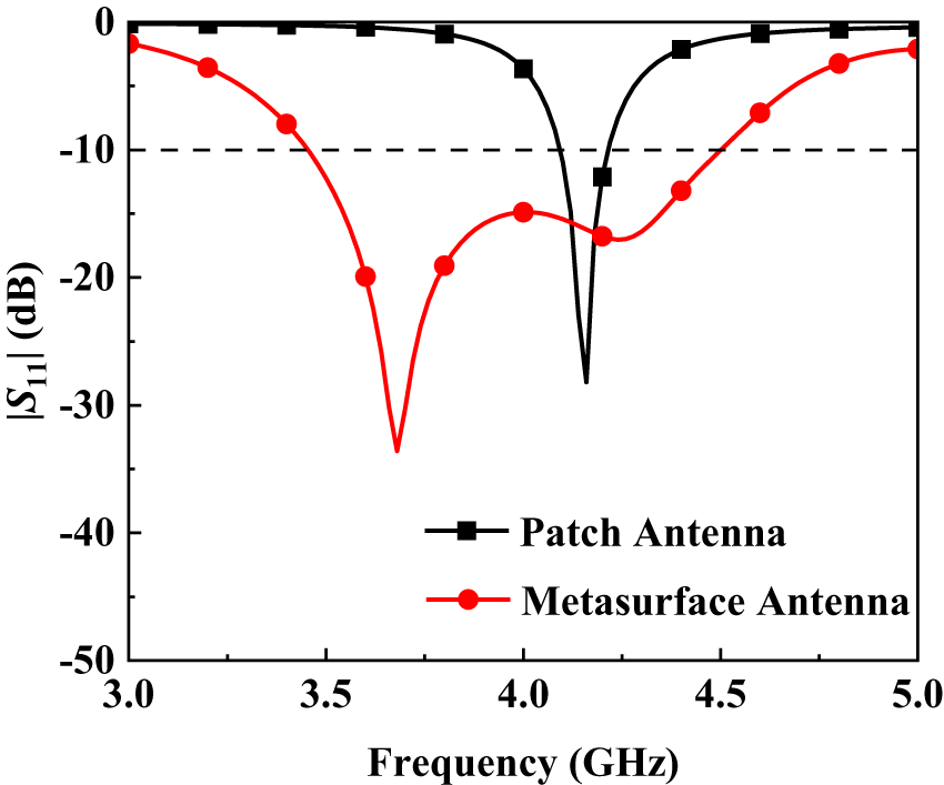
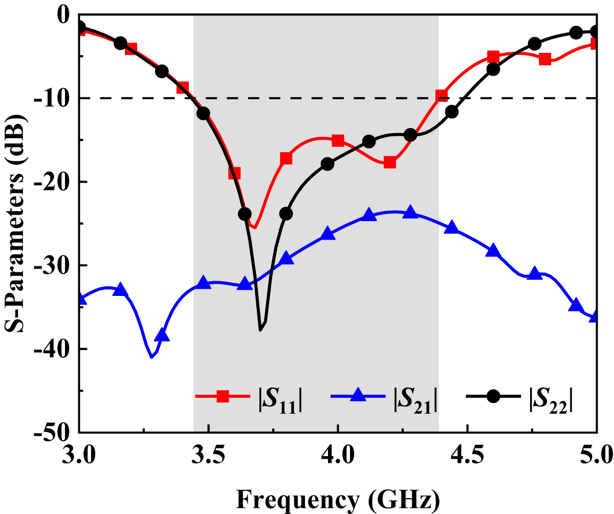
Figure 2 shows the simulated S-parameters of the patch antenna with and without MS. The feed position for each configuration was optimized to ensure good radiation performance. The results demonstrate that the unloaded patch antenna operates from 4.09 to 4.22 GHz, whereas the MS-loaded counterpart operates from 3.45 to 4.5 GHz. This indicates that the MS effectively enhances the bandwidth while maintaining structural compactness.
The simulated S-parameters of the patch antenna with and without MS.

Antenna design process using CMA
The Multilayer Solver in CST Studio Suite was utilized for the design and analysis of the antenna. First, the antenna structure was created and materials were assigned. Then, the Multilayer Solver was configured with a vacuum background and open boundary conditions. The characteristic mode count was set to four for the patch antenna and eight for both the MS and the final antenna, after which the simulation was executed. Figure 3 plots the modal significance and modal current distributions of the rectangular patch. The modal significance reflects the radiation potential, with modes having an MSv > 0.707 considered effectively excitable. As shown, the patch exhibits vertical (Mode 1, TM10) and horizontal (Mode 2, TM01) radiation modes at 4.3 and 5.9 GHz, respectively. Both modes display strong main lobe radiation, and exciting either mode can achieve satisfactory radiation performance. In contrast, Mode 3 (TM11) and Mode 4 (TM 20) are spurious resonant modes with weaker radiation capabilities.
The CMA results of the rectangular patch. (a) Modal significance. (b) Modal currents and radiation pattern.

Figure 3 Long description
Two sub-images are present. The image A showing a line graph with four plotted series and a legend listing Mode 1, Mode 2, Mode 3 and Mode 4. The x-axis label is Frequency (Gigahertz), ranging from 3 to 9 with tick marks at 3, 4, 5, 6, 7, 8 and 9. The y-axis label is Modal Significance (decibel), ranging from 0.0 to 1.0 with tick marks at 0.0, 0.2, 0.4, 0.6, 0.8 and 1.0. Mode 1 has a narrow peak labeled 4.3 near y equals 1.0, then drops to about 0.45 at about 4.5, about 0.15 at about 5.0 and rises gradually to about 0.25 at 9. Mode 2 rises to a peak labeled 5.9 near y equals 1.0, then decreases to about 0.42 at about 6.4, about 0.30 at about 6.8, about 0.28 at about 7.2 and is about 0.30 at 9. Mode 3 stays near 0 until about 6.5, then rises to a narrow peak labeled 7.6 near y equals 1.0, then drops to about 0.45 at about 7.8 and to about 0.18 at 9. Mode 4 stays near 0 until about 7.0, then rises to a peak labeled 8.4 near y equals 1.0, then decreases to about 0.55 at about 8.8 and about 0.40 at 9. The image B showing four rectangular vector-field plots arranged left to right, each with many small arrows and one or more thick black arrows overlaid. Beneath each rectangle is a label reading Mode1, Mode2, Mode3 and Mode4, respectively. Between the second and third rectangles, a small axis triad is shown with x pointing right, y pointing up and z pointing down-left. In the first rectangle, a single thick black arrow points upward near the center. In the second rectangle, one thick black arrow points left near the middle and another thick black arrow points upward near the top. In the third rectangle, thick black arrows point right near the top, down along the left side, up along the right side and left near the bottom. In the fourth rectangle, one thick black arrow points upward near the top center and another thick black arrow points downward near the bottom center. Below the rectangles are four small circular radiation-pattern style images aligned with the four modes.
Additionally, Fig. 4 illustrates the modal significance and modal currents distributions of the initial 3 × 3 MS. As shown in Fig. 4(a), Modes 1 and 2 constitute a pair of degenerate modes. Figure 4(b) reveals that Modes 1 and 2 exhibit uniformly aligned current distributions across the MS, enabling their broadside radiation with well-defined main lobes. In contrast, Modes 3–8 display diverse current orientations and radiation patterns dominated by sidelobes, rendering them unsuitable as primary radiating modes.
The CMA results of the original MS. (a) Modal significance. (b) Modal currents and radiation pattern.

Figure 4 Long description
A composite figure with two parts. The image A showing a line graph. The y-axis label is Modal Significance (dB). The y-axis ranges from 0.0 to 1.0 with labeled ticks at 0.0, 0.2, 0.4, 0.6, 0.8 and 1.0. The x-axis label is Frequency (GHz). The x-axis ranges from 3 to 9 with labeled ticks at 3, 4, 5, 6, 7, 8 and 9. A thick black curve rises from near 0 at 3 GHz, increases gradually through 4 to 5 GHz, reaches a narrow peak near 6 GHz close to 1.0, then drops steeply to near 0 by about 7 GHz and stays near 0 through 9 GHz. Square markers are plotted along the black curve, including multiple markers on the rising section, several around the peak and several on the falling section. Several light dashed curves are also plotted, clustered around the peak region and extending across the frequency range. Two numeric labels, 5.6 and 6.7, appear near the top of the plot and a vertical dotted line is drawn near 6 GHz. The image B showing eight mode blocks labeled Mode1 through Mode8. Each mode block contains a square grid of small vector-field tiles with arrows and a circular radiation-pattern style plot below the grid. A small axis triad labeled x, y, z appears near the center between the upper and lower rows. Mode1 and Mode2 show circular plots with a single central lobe. Mode3 and Mode4 show circular plots with a ring-like feature around a central region. Mode5 and Mode6 show circular plots with multiple rounded lobes around the perimeter. Mode7 shows a circular plot with many lobes around the perimeter. Mode8 shows a circular plot with two larger lobes on opposite sides.
To optimize radiation performance, the design aims to jointly excite a mode in the rectangular patch with its corresponding MS mode, requiring their modal currents to be aligned. To achieve this alignment, three horizontal slots were introduced into the three central patches of the initial MS. The slot widths are identical to those of the inter-unit gaps. Figure 5 illustrates the modal significance and modal current distributions of this modified MS. The results show that the slots not only separate the two degenerate modes but also reconfigure their current directions to horizontal (Mode 1) and vertical (Mode 2), respectively, thereby achieving the required current alignment for joint excitation with the patch.
The CMA results of the proposed MS. (a) Modal significance. (b) Modal currents and radiation pattern.

Figure 5 Long description
The image A showing a line graph with the y-axis labeled Modal Significance (dB) and tick labels 0.0, 0.2, 0.4, 0.6, 0.8, 1.0. The x-axis is labeled Frequency (GHz) with tick labels 3, 4, 4.8, 5, 5.2, 6, 7, 8, 9. One curve labeled Mode 1 rises from near 0.0 at 3 GHz to about 0.1 at 4 GHz, then increases steeply to about 1.0 near 5.0 GHz and then drops to near 0.0 by about 6.8 to 7.0 GHz. A second curve labeled Mode 2 rises from near 0.0 at 3 GHz to about 0.2 at about 4.5 GHz, reaches about 0.9 near about 5.0 GHz, reaches about 1.0 near about 5.2 GHz, then decreases to about 0.45 near 6.0 GHz and continues decreasing to about 0.35 near 7.0 GHz, about 0.30 near 8.0 GHz and about 0.27 near 9.0 GHz. Several additional faint curves are present and an arrow label indicates Mode 3 dash 8. The image B showing eight mode blocks labeled Mode1, Mode2, Mode3, Mode4 on the top row and Mode5, Mode6, Mode7, Mode8 on the bottom row. Each mode block contains a rectangular grid of small vector-field style subcells with arrows and a separate radiation-pattern style shape below the grid. A small axis triad labeled x, y, z appears near the Mode2 and Mode3 area. The radiation-pattern shapes are shown as filled lobed forms: Mode1 is a single rounded lobe; Mode2 is a single rounded lobe; Mode3 is a two-lobed shape with a narrow center; Mode4 is a single rounded lobe with a central spot; Mode5 is a vertically elongated lobe; Mode6 is a single rounded lobe with a central spot; Mode7 is a four-lobed shape; Mode8 is a four-lobed shape with broader lobes.
Figure 6 shows the CMA results of the integrated MS and rectangular patch structure. To simultaneously visualize their modal current distributions, bottom views are shown inverted in Fig. 6(b). The results indicate that the integrated structure exhibits vertical (Mode 1) or horizontal (Mode 2) current distributions on both the patch and MS. Both modes maintain radiation patterns with well-defined main lobes. The modal significance curves in Fig. 6(b) show that these modes resonant at 3.64 GHz (Mode 1) and 4.0 GHz (Mode 2), respectively. Compared with the resonant frequencies of the standalone rectangular patch in Fig. 3, Mode 1 of the integrated structure resonates closer to the patch’s frequency than Mode 2 does. This closer frequency alignment facilitates stronger joint excitation between the MS and the patch, which is why Mode 1 was selected for the final design.
The CMA results of the proposed MS antenna. (a) Modal significance. (b) Modal currents and radiation pattern.

Figure 6 Long description
The image A showing a line graph with a legend listing Mode 1 and Mode 2 and a text label reading Mode 3 to 8. The x-axis label is Frequency (gigahertz), with tick labels 3, 3.6, 4, 5, 6, 7, 8, 9. The y-axis label is Modal Significance (decibel), ranging from 0.0 to 1.0 with tick labels 0.0, 0.2, 0.4, 0.6, 0.8, 1.0. Mode 1 is plotted with square markers on a curve that rises from about 0.15 at 3 gigahertz to about 0.67 near 3.6 gigahertz, reaches about 1.0 just below 4 gigahertz, then drops to about 0.42 at 4 gigahertz and to near 0 by about 4.3 gigahertz, staying near 0 from about 4.5 to 9 gigahertz with small values around 0.01 to 0.03 between about 6 and 7.5 gigahertz. Mode 2 is plotted with square markers on a curve that rises from about 0.15 at 3 gigahertz to about 0.5 near 3.6 gigahertz, reaches about 1.0 near 4 gigahertz, then decreases to about 0.85 near 4.5 gigahertz, about 0.7 near 5 gigahertz, about 0.18 near 5.6 gigahertz and approaches 0 by about 6 gigahertz. The image B showing two groups of arrow-field diagrams labeled Mode1 and Mode2, plus two circular radiation-pattern images below them. At left, Mode1 shows a central rectangular region with many arrows pointing upward, surrounded by smaller rectangular regions also containing arrows, with several large black arrows pointing upward over the rectangles. A coordinate triad is shown nearby with x and y labeled and z indicated with a circled cross symbol. At right, Mode2 shows a grid of rectangular regions filled with arrows, with several large black arrows pointing left over the rectangles. Below, two separate circular plots appear, one under Mode1 and one under Mode2, each showing a filled circular shape with concentric rings. A second coordinate triad appears near the lower left with x, y and z labeled.
Single-port MS antenna with coaxial feed
Based on the CMA in the previous section, a 50 Ω coaxial probe is proposed for exciting modes 1. Figure 7 illustrates the current distributions of the excited antenna at resonant frequencies of 3.68 and 4.26 GHz. As shown, the distribution at 3.68 GHz matches that of Mode 1 in the integrated patch-MS structure from Fig. 6. At 4.26 GHz, the current is primarily concentrated on the rectangular patch, which is identical to Mode 1 of the standalone patch in Fig. 3. These results are in line with the expected design.
The current distributions at 3.68 and 4.36 GHz of the single-port MS antenna.

Figure 7 Long description
A two-part surface current density vector-field plot on a rectangular antenna layout, shown at two frequencies. A direction indicator shows x, y and z. No plotted x-axis or y-axis with numeric scales are shown. A vertical legend is labeled Jsurf in A slash m, with tick labels 0.2, 4.2, 8.1, 12.1, 16.0 and 20.0. Small arrows across each map indicate surface current direction and the legend indicates surface current density magnitude. The image A showing the frequency label 3.68 gigahertz. The layout includes a central vertical rectangular region and multiple surrounding rectangular regions separated by narrow gaps. The central region contains dense small arrows that are mostly aligned upward, plus one large black arrow pointing upward. Four surrounding regions each include a large black arrow pointing upward. Several surrounding regions show curved arrow patterns near the inner corners. A small red circular marker appears near the upper part of the central region. The image B showing the frequency label 4.26 gigahertz. The same layout is shown. The central region contains dense small arrows that are mostly aligned upward, plus one large black arrow pointing upward. Many surrounding regions show curved arrow patterns, with numerous arrows changing direction around the gaps between regions. A small red circular marker appears near the upper part of the central region.
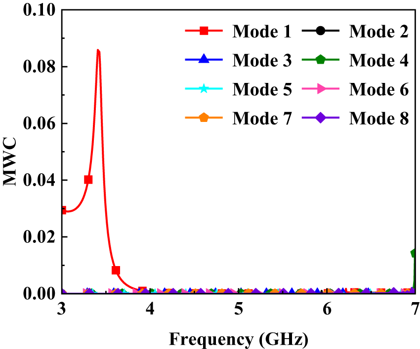
To determine the effective excitation of the port, Fig. 8 presents the modal weighting coefficient (MWC) result which is calculated by introducing the coaxial line shown in Fig. 1 and setting it as a discrete port. It can be seen that in the frequency band around 3.6 GHz, except for Mode 1, the MWC of all other modes is close to zero. Hence, only Mode 1 is effectively excited within this frequency band, which is highly consistent with the current distribution result presented in Fig. 7.
MWC of the proposed MS antenna.

Figure 8 Long description
Legend: Mode 1, Mode 2, Mode 3, Mode 4, Mode 5, Mode 6, Mode 7, Mode 8. Horizontal axis label: Frequency (GHz). Range: 3 to 7. Vertical axis label: MWC. Range: 0.00 to 0.10. Mode 1 coordinate pairs: (3.0, 0.03), (3.3, 0.04), (3.4, 0.085), (3.6, 0.008). Mode 4 coordinate pairs: (7.0, 0.015). Mode 1 shows a rise from 0.03 at 3.0 to 0.085 at 3.4, then a drop to 0.008 at 3.6. Mode 2 is plotted close to 0.00 across the frequency range 3 to 7. Mode 3 is plotted close to 0.00 across the frequency range 3 to 7. Mode 4 is plotted close to 0.00 across the frequency range 3 to 7, with a plotted point at (7.0, 0.015). Mode 5 is plotted close to 0.00 across the frequency range 3 to 7. Mode 6 is plotted close to 0.00 across the frequency range 3 to 7. Mode 7 is plotted close to 0.00 across the frequency range 3 to 7. Mode 8 is plotted close to 0.00 across the frequency range 3 to 7.
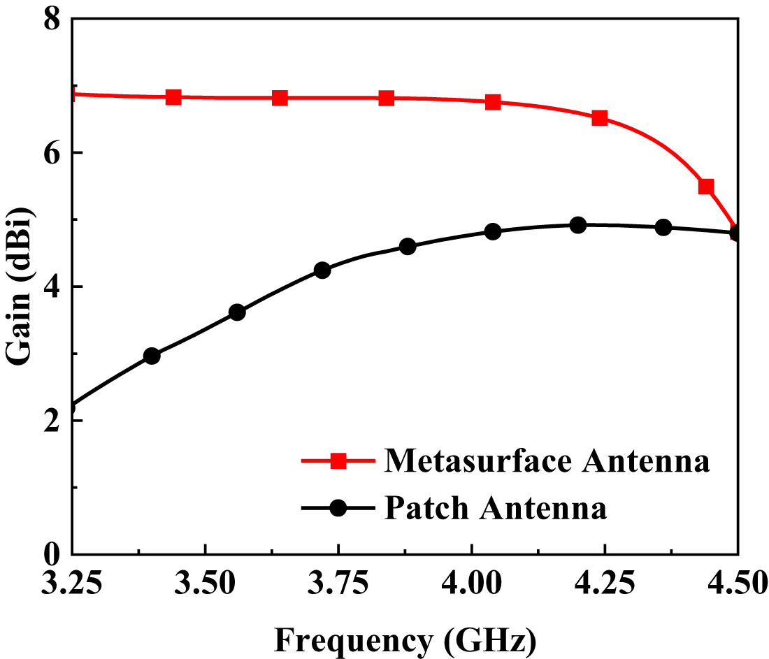
Figure 9 compares the simulated gain of the antenna with and without the MS. The original patch antenna exhibits a peak gain of 4.8 dBi within its operational band (4.09–4.22 GHz). After integrating the MS, the gain is improved to a 4.9–6.8 dBi across an expanded bandwidth of 3.45–4.5 GHz, with a gain fluctuation of less than 1.9 dB and a flat gain curve across most of the band.
The simulated gain of antenna with and without MS.

Figure 10 presents the normalized radiation patterns simulated at 3.68 and 4.26 GHz. The antenna exhibits consistent E- and H-plane radiation patterns at both frequencies, achieving quasi-omnidirectional radiation with low cross-polarization levels. The peak gains are 6.8 dBi (3.68 GHz) and 6.48 dBi (4.26 GHz), which meet the gain requirements for 5G NR applications.
The simulated normalized radiation pattern of single-port MS antenna. (a) 3.68 GHz, E-plane. (b) 3.68 GHz, H-plane. (c) 4.26 GHz, E-plane. (d) 4.26 GHz, H-plane.

Figure 10 Long description
The simulated normalized radiation pattern of a single-port MS antenna is shown in four polar plots. The radial axis represents gain in decibels, ranging from 0 to minus 60. The angle is labeled from 0 to 360 degrees in increments of 30. Image A shows the E-plane at 3.68 GHz. The co-polarization (Sim E-copol) trace follows near the outer ring, with a dip around 180 degrees. The cross-polarization (Sim E-x-pol) trace forms a smaller loop near the center, peaking around 90 degrees. Image B shows the H-plane at 3.68 GHz. The co-polarization (Sim H-copol) trace stays close to the outer ring, with a slight dip near 180 degrees. The cross-polarization (Sim H-x-pol) forms a symmetric two-lobed shape, peaking at 90 and 270 degrees. Image C shows the E-plane at 4.26 GHz. The co-polarization (Sim E-copol) trace runs near the outer ring, dipping around 180 degrees. The cross-polarization (Sim E-x-pol) forms a multi-loop shape near the center, with a larger bulge at 90 degrees. Image D shows the H-plane at 4.26 GHz. The co-polarization (Sim H-copol) trace remains near the outer ring, with a mild dip at 180 degrees. The cross-polarization (Sim H-x-pol) forms a symmetric two-lobed shape, peaking at 90 and 270 degrees. Overall, the co-polarization dominates across most angles, while cross-polarization remains significantly lower, approximately 40 to 60 decibels below the peak. The plots illustrate the antenna’s polarization purity and radiation pattern consistency across different planes and frequencies.
Dual-port MS MIMO antenna
As illustrated in Fig. 11, two of the proposed single-port MS antennas are orthogonally arranged to form a dual-port MIMO antenna. The edge-to-edge distance between the two MSs is 0.049 λ 0, where λ 0 is the free-space wavelength corresponding to the lower cutoff frequency of the antenna. The detailed parameters of the MIMO antenna are listed in Table 1.
Geometry of the dual-port MS MIMO antenna. (a) 3D. (b) Top and bottom views.

Figure 11 Long description
Insufficient visual information to describe this element accurately.
Figure 12 shows the simulated S-parameters of the MIMO antenna. As shown, the proposed MS MIMO antenna operates from 3.44 to 4.39 GHz with an isolation greater than 23.6 dB across the entire band, demonstrating inherent decoupling. By exciting the fundamental TM10, polarization diversity is achieved, enabling high isolation without additional decoupling structures.
Simulated S-parameters of the MS MIMO antenna.

Additionally, the current distributions of the MIMO antenna at 3.68 and 4.18 GHz are depicted in Fig. 13(a) and (b), respectively. When port 1 is excited, the current is primarily concentrated on the rectangular patch and the edge regions of the MS layer at both frequencies. In contrast, the coupled current on the neighboring antenna 2 is relatively weak.
Current distributions of the proposed antenna at (a) 3.68 GHz and (b) 4.18 GHz.

Figure 13 Long description
The image shows vector-field plots of surface current density for an antenna at two frequencies: 3.68 gigahertz and 4.18 gigahertz. The plots illustrate the distribution of surface current density magnitude, labeled as Jsurf in A m superscript -1, with a color scale ranging from 0.2 to 20.0 A m superscript -1. Arrows indicate the direction of surface current. Panel (a) represents the current distribution at 3.68 gigahertz. A high current region is observed near the central sections, reaching the upper range of the color scale, while other areas show lower current densities. Panel (b) shows the distribution at 4.18 gigahertz. Similar to panel (a), a high current region is present, but the peak magnitude is slightly reduced compared to panel (a). The rest of the sections display more uniformly low currents. Both panels use the same color scale and coordinate orientation, with x pointing right, y pointing down and z pointing up. The plots highlight the differences in current distribution between the two frequencies, with panel (a) showing a more pronounced peak in current density.
Fabrication and experimental results
To validate the design, a prototype of the dual-port MIMO antenna was fabricated and measured. SMA-KFD5 coaxial connectors specified for DC to 6 GHz operation was adopted. The fabricated prototype and test environment are depicted in Fig. 14. The S-parameters were measured using an Agilent N5222A vector network analyzer, and the radiation patterns were measured in an anechoic chamber.
Fabricated antenna and test environment. (a) Top view. (b) Bottom and side view. (c) Test environment.

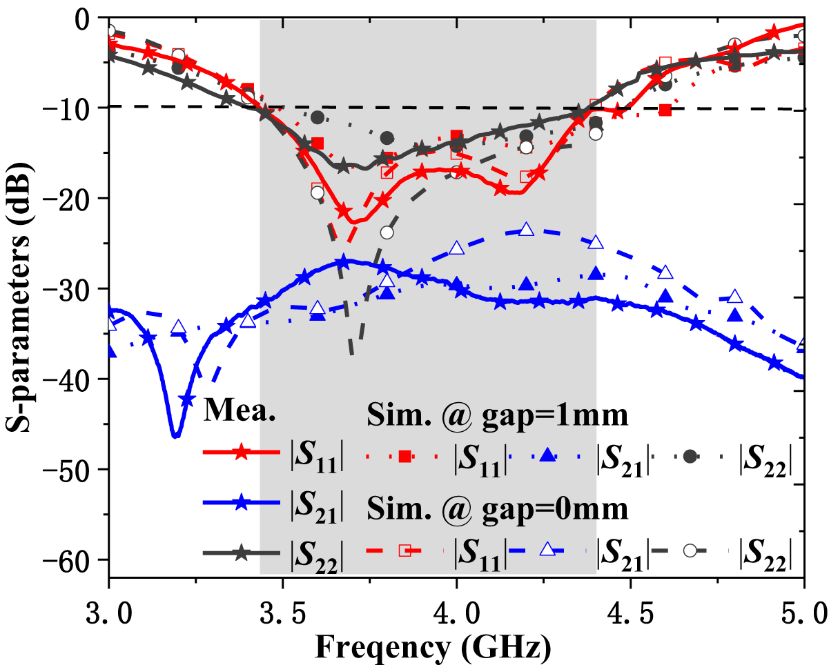
Figure 15 compares the measured and simulated S-parameters of the dual-port MIMO antenna. Good agreement is observed between the simulated and measured results, both covering an operating band of 3.44–4.39 GHz, with the measured isolation exceeding 26.25 dB across the band. The error primarily originates from manufacturing tolerances. Since the antenna consists of an MS layer and a patch layer, fabrication limitations result in a small interlayer gap at the solder joints for the SMA connector probe. This gap significantly degrades the accuracy of the measurement results. To verify this, the simulation results for a 1 mm gap between the upper and lower layers are also included in Fig. 15. It can be observed that the gap causes a frequency shift and alters the magnitude of the S-parameters. This confirms that the discrepancy between the measured and simulated results is mainly attributable to manufacturing tolerances.
Simulated and measured S-parameters of the proposed MS MIMO antenna.

Figure 15 Long description
Simulated and measured -parameters of the proposed MS MIMO antenna.S A line graph with multiple overlaid curves. The x-axis is labeled Frequency (gigahertz), with tick labels at 3.0, 3.5, 4.0, 4.5 and 5.0. The y-axis is labeled S-parameters (decibel), ranging from 0 at the top down to minus 60 at the bottom, with tick labels at 0, minus 10, minus 20, minus 30, minus 40, minus 50 and minus 60. A horizontal dashed reference line is drawn at minus 10 decibel. A vertical shaded band spans a mid-frequency region between the 3.5 and 4.5 tick marks. Legend text includes: Mea.; Sim. at gap equals 1 millimeter; Sim. at gap equals 0 millimeter. The plotted quantities in the legend are magnitude of S subscript 11, magnitude of S subscript 21 and magnitude of S subscript 22. Magnitude of S subscript 11 curves occupy the upper portion of the plot. One magnitude of S subscript 11 curve drops from near 0 decibel around 3.0 gigahertz to below minus 10 decibel within the shaded band, reaching a minimum below minus 20 decibel around the mid-band, then rises toward near 0 decibel by 5.0 gigahertz. Another magnitude of S subscript 11 curve follows a similar shape with a mid-band minimum between minus 10 and minus 20 decibel. Magnitude of S subscript 22 curves also occupy the upper portion of the plot and track near the magnitude of S subscript 11 curves. They dip below minus 10 decibel in the shaded band and rise again toward the upper range by 5.0 gigahertz. Magnitude of S subscript 21 curves occupy the lower portion of the plot. One magnitude of S subscript 21 curve shows a deep notch near the low-frequency end, reaching below minus 40 decibel shortly after 3.0 gigahertz, then rises to around the minus 30 decibel region through the shaded band and trends downward again toward the high-frequency end. Additional magnitude of S subscript 21 curves remain between roughly minus 25 and minus 40 decibel across the frequency range, with their highest levels occurring within the shaded band.
Figure 16 compares the measured and simulated radiation patterns of the prototype at 3.68 and 4.18 GHz. When port 1 is excited, port 2 is terminated by a matched load. At the two frequencies of 3.68 GHz and 4.18 GHz, the main beam directions of the antenna in the E-plane are 0° and −45°, respectively, while in the H-plane they are both close to 0°. On the main radiation direction, the cross-polarization level is more than 20 dB lower than the co-polarization. It should be noted that within the angular range of 120°–240° in the E-plane, the measured cross-polarization radiation is significantly higher than the simulation results. This discrepancy is primarily attributed to multi-path reflections and scattering from the antenna mount in the measurement environment.
The simulated and measured normalized radiation pattern of MS MIMO antenna. (a) 3.68 GHz, E-plane. (b) 3.68 GHz, H-plane. (c) 4.18 GHz, E-plane. (d) 4.18 GHz, H-plane.

Figure 16 Long description
The image consists of four polar plots comparing simulated and measured normalized radiation patterns of an MS MIMO antenna. Each plot represents different conditions: (a) 3.68 GHz in the E-plane, (b) 3.68 GHz in the H-plane, (c) 4.18 GHz in the E-plane and (d) 4.18 GHz in the H-plane. The radial axis represents gain in decibels, ranging from 0 to approximately -60. The angle axis is in degrees, ranging from 0 to 360. Each plot includes four datasets: simulated co-polarization (Sim E-copol or Sim H-copol), measured co-polarization (Mea E-copol or Mea H-copol), simulated cross-polarization (Sim E-x-pol or Sim H-x-pol) and measured cross-polarization (Mea E-x-pol or Mea H-x-pol). In the E-plane plots, the main beam direction is at 0 degrees for 3.68 GHz and -45 degrees for 4.18 GHz. In the H-plane plots, the main beam direction is close to 0 degrees for both frequencies. The cross-polarization level is more than 20 decibels lower than the co-polarization in the main radiation direction. Notable discrepancies between simulation and measurement occur in the E-plane within the angular range of 120 to 240 degrees, where measured cross-polarization is significantly higher.
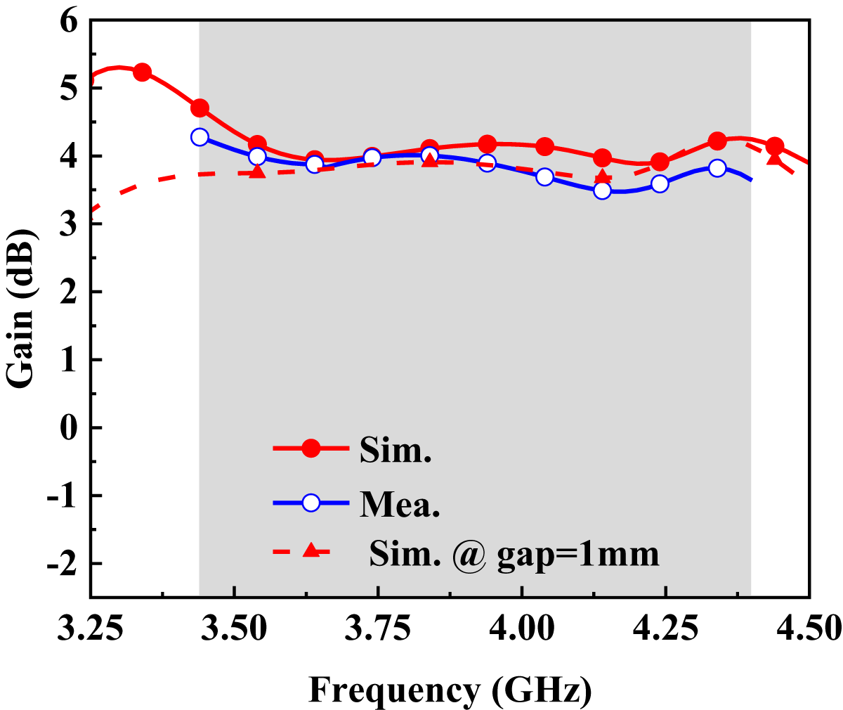
Figure 17 plots the measured and simulated gain of the MIMO antenna. Over the operating band, the simulated and measured gains range from 3.9 to 4.7 dBi and 3.43 to 4.27 dBi, with fluctuations of 0.8 dB and 0.84 dB, respectively. The results demonstrate flat gain characteristics with good agreement between simulation and measurement. The discrepancy is primarily attributed to antenna fabrication tolerances as well as non-ideal measurement conditions such as cable loss, multipath interference, and gain standard uncertainty. As mentioned above, an inevitable small gap between the MS and the feed layer degrades impedance matching and introduces additional loss. To verify the impact of this fabrication imperfection, Fig. 17 also presents the simulated gain for a 1 mm interlayer gap. The results show an overall decrease in gain compared to the case without a gap, confirming that manufacturing imperfections cause errors in gain measurement.
The simulated and measured gain of MS MIMO antenna.

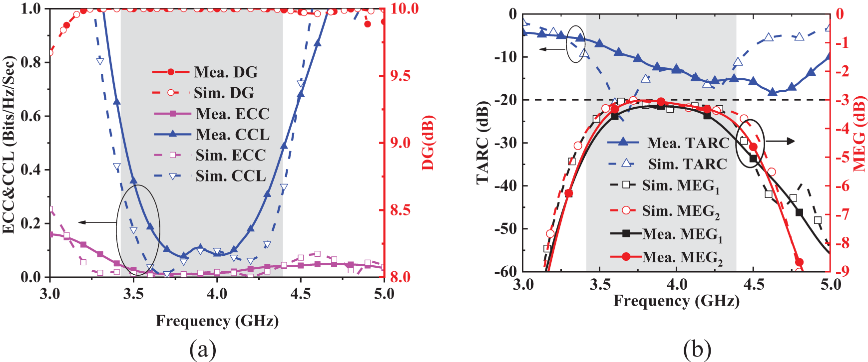
To further evaluate the diversity characteristics and data transmission quality of this MIMO antenna, Fig. 18 presents the calculated results for envelope correlation coefficient (ECC), diversity gain (DG), total active reflection coefficient (TARC), channel capacity loss (CCL), and mean effective gain (MEG). The measured and simulated values of these indicators show good agreement. In engineering practice, the generally acceptable ranges are as follows: ECC < 0.5, CCL < 0.5 bits/Hz/sec, DG > 6 dB (with10 dB being ideal), TARC < 0 dB, and MEG < −3 dB. In Fig. 18(a), within the entire operating frequency band, both measured and simulated ECC values remain below 0.05, the CCL values are under 0.48 bits/Hz/sec, and DG values exceed 9.9 dB. Meanwhile, Fig. 18(b) indicates that the TARC and MEG obtained from measurement and simulation are respectively lower than −7 dB and −3 dB. These results confirm that the proposed MIMO antenna achieves excellent spatial multiplexing performance across the entire frequency band, ensuring reliable signal transmission.
The indicators of MS MIMO antenna calculated from simulated and measured results. (a) ECC, CCL, and DG. (b) TARC and MEG.

Figure 18 Long description
The image A showing a line graph with Frequency (Gigahertz) on the horizontal axis from 3.0 to 5.0, with labeled ticks at 3.0, 3.5, 4.0, 4.5 and 5.0. The left vertical axis is labeled ECC and CCL (Bits per Hertz per Sec) from 0.0 to 1.0 with labeled ticks at 0.0, 0.2, 0.4, 0.6, 0.8 and 1.0. The right vertical axis is labeled DG (decibel) from 8.0 to 10.0 with labeled ticks at 8.0, 8.5, 9.0, 9.5 and 10.0. A legend lists six series: Mea. DG, Sim. DG, Mea. ECC, Mea. CCL, Sim. ECC and Sim. CCL. Mea. DG is a red line with filled circle markers near the top of the plot, starting near 9.7 at 3.0 Gigahertz and reaching about 10.0 by about 3.3 Gigahertz, then staying close to 10.0 through 5.0 Gigahertz, with a final point slightly below 10.0 near 5.0 Gigahertz. Sim. DG is a red dashed line with open circle markers that follows a similar path close to 10.0 across most of the range. Mea. ECC is a purple line with square markers that starts near 0.20 at 3.0 Gigahertz, decreases toward about 0.05 by about 3.4 Gigahertz, approaches about 0.00 around 3.6 to 4.2 Gigahertz, then rises slightly to around 0.05 to 0.08 near 4.6 to 5.0 Gigahertz. Sim. ECC is a purple dashed line with open square markers that stays close to 0.00 from about 3.4 to 4.4 Gigahertz and rises slightly above 0.05 near the upper end of the frequency range. Mea. CCL is a blue line with filled triangle markers that is high near 3.0 Gigahertz, drops steeply to near 0.10 around 3.6 to 4.1 Gigahertz, then rises again toward higher values by about 4.6 to 5.0 Gigahertz. Sim. CCL is a blue dashed line with open inverted triangle markers that follows a similar U shaped pattern, with low values near the middle frequencies and higher values toward the lower and upper ends. The image B showing a line graph with Frequency (Gigahertz) on the horizontal axis from 3.0 to 5.0, with labeled ticks at 3.0, 3.5, 4.0, 4.5 and 5.0. The left vertical axis is labeled TARC (decibel) from minus 60 to 0 with labeled ticks at minus 60, minus 50, minus 40, minus 30, minus 20, minus 10 and 0. The right vertical axis is labeled MEG (decibel) from minus 9 to 0 with labeled ticks at minus 9, minus 8, minus 7, minus 6, minus 5, minus 4, minus 3, minus 2, minus 1 and 0. A horizontal dashed line is drawn at minus 20 on the TARC axis and at minus 3 on the MEG axis. A legend lists six series: Mea. TARC, Sim. TARC, Sim. MEG subscript 1, Sim. MEG subscript 2, Mea. MEG subscript 1 and Mea. MEG subscript 2. Mea. TARC is a blue line with filled triangle markers, starting near minus 5 at 3.0 Gigahertz, decreasing to around minus 15 by about 4.2 Gigahertz, then rising slightly toward about minus 10 by 5.0 Gigahertz. Sim. TARC is a blue dashed line with open triangle markers, starting near minus 5 at 3.0 Gigahertz, dropping to around minus 20 near about 3.6 Gigahertz, then rising toward about minus 5 by about 4.8 to 5.0 Gigahertz. Sim. MEG subscript 1 is a black dashed curve that rises from near minus 60 at 3.0 Gigahertz to around minus 22 near about 3.6 to 4.0 Gigahertz, then falls toward about minus 55 by 5.0 Gigahertz. Sim. MEG subscript 2 is a red dashed curve that follows a similar arch shape, reaching around minus 20 near about 3.7 to 4.1 Gigahertz and then decreasing toward lower values by 5.0 Gigahertz. Mea. MEG subscript 1 is a black solid curve with square markers that rises from near minus 60 at 3.0 Gigahertz to around minus 22 near about 3.7 to 4.1 Gigahertz, then decreases to around minus 50 to minus 55 by 5.0 Gigahertz. Mea. MEG subscript 2 is a red solid curve with filled circle markers that rises from near minus 60 at 3.0 Gigahertz to around minus 20 near about 3.7 to 4.1 Gigahertz, then decreases more steeply after about 4.4 Gigahertz, reaching near minus 60 by about 4.8 to 5.0 Gigahertz.
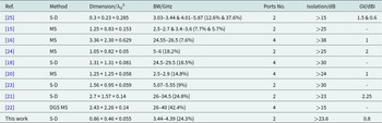
To emphasize the superior performance of the proposed antenna, Table 2 compares its performance with those reported in previous literature. Here, λ 0 denotes the free-space wavelength corresponding to the antenna’s lower cutoff frequency. The designs in [Reference Wang, Li and Yin14, Reference Zeng, Chen and Liang20, Reference Li, Nan, Xu, Chen and Feng23] have similar profile heights but occupy a much larger area. The design in [Reference Angadi, Sharma, Raghava and Sabapathy25] has a profile height approximately five times greater than that of the proposed antenna, although it achieves the smallest footprint. The antennas in [Reference Tiwari, Gaur, Kaushik, Shastri, Singh and Gahlaut21] and [Reference Gaur, Tiwari, Kaushik, Mishra, Shastri and Gahlaut22] have demonstrated superior performance in terms of bandwidth; however, their dimensions and profile are also significantly larger than those of this work. Consequently, the proposed design achieves significant miniaturization while also exhibiting superior gain flatness. In summary, by jointly exciting the TM10 mode of the rectangular patch and the MS, this work realizes a compact, high-isolation, self-decoupling MS MIMO antenna.
Comparison between the proposed and previously reported MS MIMO antennas

Table 2 Long description
The table compares multiple MIMO antenna designs by decoupling method, normalized size, operating bandwidth in gigahertz, number of ports, isolation in decibels, and gain variation in dBi. The proposed design (“This work”) is a 2-port self-decoupled antenna with a normalized size of 0.86 by 0.46 by 0.055, covering 3.44 to 4.39 GHz with 24.3 percent fractional bandwidth. Its isolation is above 23.6 dB and its gain variation is 0.8 dBi. Among other 2-port entries, isolation ranges from above 15 dB to above 30 dB, with bandwidths spanning narrow dual bands (for example 2.5 to 2.7 and 3.4 to 3.6 GHz) to wider single bands (for example 5 to 6 GHz). Several 4-port designs target millimeter-wave bands such as 24.5 to 29.5 GHz and 26 to 40 GHz, often reporting higher isolation (up to above 38 dB) but with larger normalized dimensions. Gain variation is not consistently reported across studies, so comparisons on that metric are limited to rows where values are provided.
S-D, self-decoupled; MS, MS; BW, bandwidth; GV, gain variation.
Conclusion
This paper proposes a gain-flattened MS MIMO antenna based on CMA. By analyzing the modal characteristics of the rectangular patch and MS, a pair of degenerate modes in the MS is separated, while the dominant mode is reconfigured into the desired TM10 mode. The joint excitation of the TM10 mode in both the rectangular patch and the MS enables broadband single-mode radiation. Furthermore, a compact MS MIMO antenna with self-decoupling capability via polarization diversity is constructed by orthogonally arranging the aforementioned single-port antennas. The proposed design exhibits isolation greater than 23.6 dB and a flat in-band gain variation of merely 0.8 dB. It operates from 3.44 to 4.39 GHz, fully encompassing the target 5G NR n48 band (3.55–3.7 GHz). A prototype of the MIMO antenna was fabricated and measured, confirming stable radiation patterns and reliable signal transmission performance. This work provides an effective solution for 5G wireless communication systems. Future work will explore bandwidth extension or dual-band configurations to address a broader range of sub-6 GHz and mmWave frequencies, thereby supporting more diverse 5G applications.
Acknowledgements
This work was supported by the National Natural Science Foundation of China (62071282) and the Fundamental Research Program of Shanxi Province (202203021211295).
Competing interests
The authors declare none.

Jinrong Su was born in 1981. She received the B.S. and M.S. degrees in electronic engineering and the Ph.D. degree in radio physics from Shanxi University, Taiyuan, China, in 2004, 2007, and 2017, respectively. She is currently an Associate Professor with the Department of Electronics and Information Engineering, Shanxi University. Her research interests include microwave and millimeter-wave passive device.

ShiQi Di was born in 1997. She received the B.S. degree in communication engineering and the M.S. in the Department of Information and Communication Engineering from Shanxi University, Taiyuan, China, in 2021 and 2025, respectively. Her research interests include high isolation MIMO antenna.

Xinwei Chen received the B.S. and Ph.D. degrees in electronic engineering from Shanxi University, Taiyuan, China, in 2002 and 2013, respectively. He is currently an Associate Professor with the School of Physics and Electronic Engineering, Shanxi University. His research interests include microwave and millimeter-wave passive device.

Runbo Ma was born in Changzhi, Shanxi, China, in 1974. He received the B.S., M.S., and Ph.D. degrees in electronic engineering from Shanxi University, Taiyuan, China, in 1993, 2002, and 2011, respectively. He is currently an Associate Professor with the College of Physics and Electronics, Shanxi University. His research interests include microwave and millimeter-wave integrated circuits, RFID, and microstrip antenna.

Wenmei Zhang was born in 1969. She received the B.S. and M.S. degrees in radio technology and electromagnetic field and microwave technology from the Nanjing University of Science and Technology, Nanjing, China, in 1992 and 1995, respectively, and the Ph.D. degree in electronic engineering from Shanghai Jiao Tong University, Shanghai, China, in 2004. In 2008 and 2010, she was a Senior Visiting Scholar with the Nanyang University of Technology, Singapore. She holds 6 Chinese patent, has authored more than 150 papers in peer-reviewed journals, more than 30 papers in conference proceedings. She is currently a Professor with the School of Physics and Electronics, Shanxi University, Taiyuan, China. Her current research interests include microwave/millimeter wave integrated circuits, EMC, and microstrip antenna. Prof. Zhang served as the General Chair of “2019 Cross Strait Quad-Regional Radio Science and Wireless Technology Conference” and TPC member for multiple conferences.