1. Introduction
Considering a compressible turbulent boundary layer on a flat plate, we distinguish three characteristic flow regions: viscous and logarithmic sublayers near the wall and an outer region of the boundary layer. Each of them in the framework of the Reynolds equations is described by its own approximate system of equations and its own similarity laws. For the outer region of interest, the velocity defect law is known (Fernholz Reference Fernholz1969; Fernholz & Finley Reference Fernholz and Finley1980; Smits & Dussauge Reference Smits and Dussauge2006) as follows:
 \begin{align} \frac {2 [\varphi (u_\infty ) - \varphi (\overline u)]}{M_\infty \sqrt {r (\gamma - 1) C_{\!f}}} &= - 4.7 \ln \frac y {\varDelta ^*} - 6.74, \end{align}
 \begin{align} \varphi (x) = \arcsin \frac {r u_\infty x + h_w - h_r}{\sqrt {2 r u_\infty ^2 h_w + (h_w - h_r)^2}}, & \quad \varDelta ^* = \frac {2 \int _0^\infty [\varphi (u_\infty ) - \varphi (\overline u)]\,\textrm {d} y}{M_\infty \sqrt {r (\gamma - 1) C_{\!f}}}. \end{align}
Here,
 $C_{\!f}$
is the skin-friction coefficient,
 $u_\infty$
,
 $h_\infty$
and
 $M_\infty$
are the free-stream velocity, enthalpy and Mach number,
 $h_w$
is the gas enthalpy at the wall,
 $h_r = h_\infty + r u_\infty^2/2$
is the recovery enthalpy,
 $r$
is the recovery factor, which is assumed to be
 $0. 896$
,
 $\overline u$
is the Reynolds-averaged velocity profile and
 $y$
is the distance from the wall. Comparison with a large body of experimental data (Fernholz & Finley Reference Fernholz and Finley1980) has shown that this formula approximates well the velocity profiles in a significant part of the boundary layer. At the same time, it has a substantial drawback. Relation (1.1) proposed for compressible boundary layers at small free-stream Mach numbers should obviously coincide with the von Kármán velocity defect law (Yaglom Reference Yaglom1979), which is valid for an incompressible fluid
 \begin{align} \frac {u_\infty - \overline u}{u_\infty \sqrt {\frac {1}{2} C_{\!f}}} = g \left ( \frac {y}{\delta ^*} \sqrt {\frac {1}{2} C_{\!f}} \right )\!, \quad g (\eta ) \to - \frac 1 \varkappa \ln \eta + \ldots , \quad \eta \to 0, \end{align}
where
 $\delta ^*$
is the displacement thickness,
 $\varkappa$
is the von Kármán constant and the boundary-layer thickness introduced by Clauser (Reference Clauser1956) is used as the transverse scale. Meanwhile, this is not the case. In the particular case of a thermally insulated plate, (1.2) takes the form
 \begin{align} \varphi (x) = \arcsin \frac {M_\infty x}{u_\infty } \sqrt {\frac {r (\gamma - 1)}{2 + r (\gamma - 1) M_\infty ^2}}, \end{align}
which implies that as
 $M_\infty \to 0$
, the left-hand side of (1.1) is equal to the left-hand side of equality (1.3) while
 $\varDelta ^* = \delta ^* \sqrt {2/C_{\!f}}$
. But the right-hand side of (1.1) is significantly different from that of (1.3) because
 $4.7$
is not equal to
 $1/\varkappa$
. Therefore, relation (1.1) can hardly be regarded as a valid theoretical result.
The velocity profile in the outer region was also analysed on the basis of the law of the wake proposed by Coles (Reference Coles1956) for the incompressible boundary layer, which was modified using the Van Driest (Reference Van Driest1951) formula (see, e.g. Fernholz Reference Fernholz1969; Fernholz & Finley Reference Fernholz and Finley1980; Huang, Bradshaw & Coakley Reference Huang, Bradshaw and Coakley1993; Smits & Dussauge Reference Smits and Dussauge2006; Wenzel et al. Reference Wenzel, Selent, Kloker and Rist2018; Hasan et al. Reference Hasan, Larsson, Pirozzoli and Pecnik2024; Appelbaum et al. Reference Appelbaum, Gibis, Pirozzoli and Wenzel2025).
As for the temperature profile, we do not know any analogues of the known temperature defect law for the incompressible boundary layer (Rotta Reference Rotta1964; Squire Reference Squire1964; Yaglom Reference Yaglom1979; Vigdorovich Reference Vigdorovich2015) or other similarity relations for this quantity that are valid in the outer region.
Our goal is to obtain similarity laws for velocity and temperature that are valid in the outer region of the turbulent boundary layer on a flat plate at moderate supersonic free-stream Mach numbers without involving partial hypotheses and approximate turbulence models in the way that was done for an incompressible fluid by Vigdorovich (Reference Vigdorovich2015, Reference Vigdorovich2016, Reference Vigdorovich2017). The asymptotic theory developed by Vigdorovich (Reference Vigdorovich2015, Reference Vigdorovich2016, Reference Vigdorovich2017) includes the formulation of closure relations connecting the turbulent shear stress and turbulent heat flux to the mean velocity and temperature gradients, and a special change of variables in the boundary-layer equations that makes it possible to search for the solution to the problem in the form of asymptotic expansions at large values of the logarithm of the Reynolds number based on the boundary-layer thickness (Vigdorovich Reference Vigdorovich1993). It was possible to generalise this theory to the case of gas flow (Vigdorovich Reference Vigdorovich2023a ,Reference Vigdorovich b , Reference Vigdorovich2024). In Vigdorovich (Reference Vigdorovich2023a ), strict closure relations are obtained from first principles that take into account key processes in compressible flows – a change in density and kinetic heating. Furthermore, a similar change of variables in the compressible-boundary-layer equations as well as a procedure for constructing the solution in the outer region in the form of asymptotic expansions for large values of the logarithm of Reynolds number are proposed in the present work.
A working tool of the theory is the method of matched asymptotic expansions (Van Dyke Reference Van Dyke1975), which is applied to the solutions obtained in the adjacent regions of the boundary layer – outer and logarithmic. In the latter one, the Crocco integral, which expresses a functional relation between velocity and temperature, and asymptotic expansions for the velocity and temperature profiles – the laws of the wall for these quantities, obtained by Vigdorovich (Reference Vigdorovich2023b , Reference Vigdorovich2024), are valid. The results of matching are the velocity and temperature defect laws, skin-friction law and expressions for the recovery and Reynolds-analogy factors. These relations are valid at moderate supersonic free-stream Mach numbers, when the relative difference in temperature across the boundary layer is of order one. The case of hypersonic flow in the outer region will be considered in the next paper.
Recovery and Reynolds-analogy factors are important quantitative characteristics of turbulent near-wall flow because they allow the recovery temperature and wall heat flux to be calculated from the known free-stream parameters, wall enthalpy and skin friction. Using a semi-empirical approximation of shear stress in the boundary layer, Van Driest (Reference Van Driest1956, Reference Van Driest1959) obtained expressions for these quantities in the form of expansions in the small parameter – the root of the skin-friction coefficient. The leading terms of the expansions for the recovery and Reynolds-analogy factors are found to be
 $\sigma$
and
 $1/\sigma$
, respectively, where
 $\sigma$
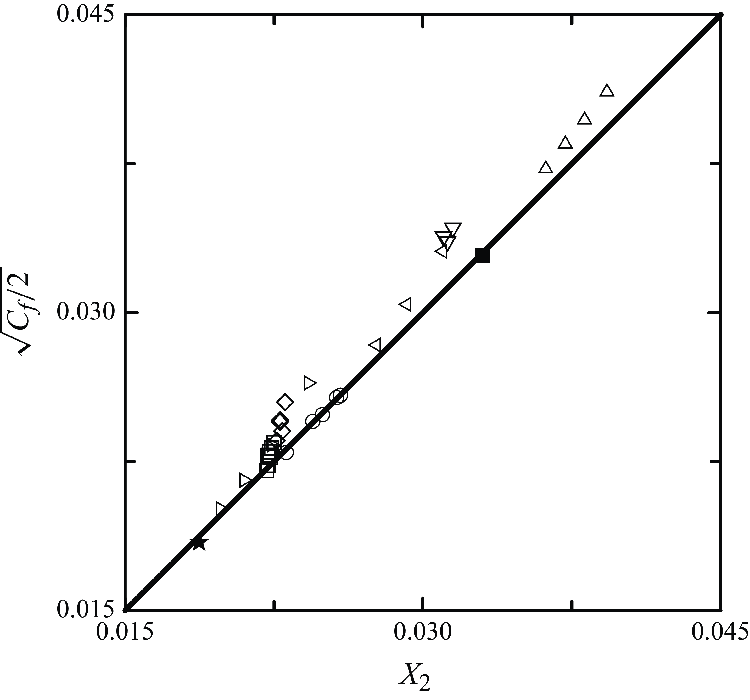
is the turbulent Prandtl number in the logarithmic region, which coincides with the asymptotic representations obtained in the present work. The skin-friction law obtained by asymptotic matching of the solutions for the outer region and logarithmic sublayer is also close in structure to the formula proposed by Van Driest (Reference Van Driest1956).
For matching, it is necessary to know asymptotic expansions of the solutions for the outer region and the logarithmic sublayer, valid at the boundaries of the two adjacent regions, which together constitute an overlap zone of the solutions. In our approach, these asymptotic expansions are uniquely determined by solving a closed boundary-value problem for the mean velocity and enthalpy fields. It can be compared with the method used by He et al. (Reference He, Kazakia and Walker1995, Reference He, Kazakia, Ruban and Walker1996), who considered the same problem of a supersonic turbulent boundary layer on a plate. These authors, however, as well as a number of their predecessors, dealt with the unclosed turbulent boundary-layer and energy equations. In this case, there is not enough data to determine the asymptotic behaviour of the velocity and enthalpy profiles in the overlap zone and, therefore, its form has to be postulated based on certain hypotheses. He et al. (Reference He, Kazakia and Walker1995, Reference He, Kazakia, Ruban and Walker1996), in particular, assumed that velocity in the logarithmic region of supersonic boundary layers in terms of a rescaled transverse coordinate obeys a logarithmic law, just as in an incompressible fluid. Meanwhile, as proved by Vigdorovich (Reference Vigdorovich2024), this is not the case and in the leading term of the asymptotic expansion the velocity profile is described by the well-known Van Driest (Reference Van Driest1951) formula. An incorrect asymptotics is also chosen for enthalpy in the near-wall region. Naturally, the consequences of incorrect assumptions give incorrect results.
The following § 2 gives the problem formulation, basic equations and closure relations. In § 3 the outer region of the boundary layer is considered, the velocity and temperature profiles in which are constructed as asymptotic expansions at large values of the logarithm of the Reynolds number based on the boundary-layer thickness. Section 4 presents the main similarity relationships valid in the logarithmic region adjacent to the outer region of the boundary layer: the Crocco integral and the laws of the wall for velocity and temperature. They are needed for asymptotic matching with the solution in the outer region, as a result of which in § 5 the velocity defect law (§ 5.1) and temperature defect law (§ 5.2) for the outer region are obtained. Other results of the matching are asymptotic expansions for the recovery (§ 6.1) and Reynolds-analogy (§ 6.2) factors. In § 7 the velocity and temperature defect laws are formulated that are valid everywhere outside the viscous sublayer. The formulations of similarity rules for the Reynolds-tensor components and root-mean-square enthalpy fluctuation are given in § 8 while the skin-friction law valid for zero and non-zero wall heat flux is presented in § 9.
2. Basic equations and closure relations
We consider a turbulent boundary layer on a flat plate in a uniform stationary stream with velocity
 $u_\infty$
, density
 $\rho _\infty$
, viscosity
 ${\mu} _\infty$
and enthalpy
 $h_\infty$
. The gas enthalpy at the plate
 $h_w$
is constant. The gas is perfect with heat capacity ratio
 $\gamma$
. The coefficients of viscosity
 ${\mu}$
and thermal conductivity
 $k$
are power functions of temperature with the exponent
 $n$
, while the molecular Prandtl number
 $\textit{Pr} = c_p {\mu} /k$
is a constant quantity.
The flow is described by the compressible turbulent boundary-layer equations
 \begin{align} \overline \rho \tilde u \frac {{\partial } \tilde u} {{\partial } x} + \overline \rho \tilde v \frac {{\partial } \tilde u} {{\partial } y} = \frac {{\partial }} {{\partial } y} & \left ( \overline {{\mu} \frac {{\partial } u} {{\partial } y}} - \overline \rho \, \widetilde {u'' v''} \right )\!, \end{align}
 \begin{align} \frac {{\partial } \overline \rho \tilde u} {{\partial } x} + \frac {{\partial } \overline \rho \tilde v}{{\partial } y} = 0, &\end{align}
 \begin{align} \overline \rho \tilde u \frac {{\partial } \tilde h} {{\partial } x} + \overline \rho \tilde v \frac {{\partial } \tilde h} {{\partial } y} = \frac {\partial } {{\partial } y} \left [ \overline { \frac k {c_p} \frac {{\partial } h} {{\partial } y}} + \overline {{\mu} u \frac {{\partial } u} {{\partial } y}} - \overline \rho \widetilde {h'' v''} \right. & \left. -\, \frac {\overline \rho } 2 \left(\widetilde {u^{\prime \prime 2} v''} + \widetilde {v^{\prime \prime 3}} + \widetilde {v'' w^{\prime \prime 2}}\right) \right ] \nonumber \\- \tilde u \frac {{\partial }} {{\partial } y} \left ( \overline {{\mu} \frac {{\partial } u} {{\partial } y}} \right ) & - \overline \rho \frac {{\partial } \tilde u} {{\partial } y}\, \widetilde {u'' v''}, \\\overline \rho \, \tilde h = \frac {\gamma p_\infty }{(\gamma -1)}; & \nonumber \\x \gt 0, \quad y = 0: \quad \tilde u = \tilde v = 0, \quad \tilde h = h_w; \quad y \to \infty : &\quad \tilde u \to u_\infty , \quad \tilde h \to h_\infty , \nonumber \end{align}
in which Favre’s averaging (Favre Reference Favre1969) with density as a weighting function is used. As shown by Vigdorovich (Reference Vigdorovich2023a ), in the energy equation (2.1c ), the terms associated with the triple correlations of velocity fluctuations, which are usually neglected, should be retained (see also Huang, Coleman & Bradshaw Reference Huang, Coleman and Bradshaw1995; Wenzel, Gibis & Kloker Reference Wenzel, Gibis and Kloker2022).
We use the relations
 \begin{align} \widetilde {u'' v''} = - \left ( y \frac {{\partial } \tilde u}{{\partial } y} \right )^2 & S ({\textit{Re}},\, {\textit{Pe}},\, n,\, \eta ,\, \varPi _1,\, \varPi _2,\, \varGamma ), \end{align}
 \begin{align} \widetilde {h'' v''} + \frac {1}{2} \left ( \widetilde {u^{\prime \prime 2} v''} + \widetilde {v^{\prime \prime 3}} +\widetilde {v'' w^{\prime \prime 2}} \right ) &= - y^2 \frac {{\partial } \tilde h}{{\partial } y} \frac {{\partial } \tilde u}{{\partial } y}H ({\textit{Re}},\, {\textit{Pe}},\, n,\, \eta ,\, \varPi _1,\, \varPi _2,\, \varGamma ) \\[9pt] \nonumber \end{align}
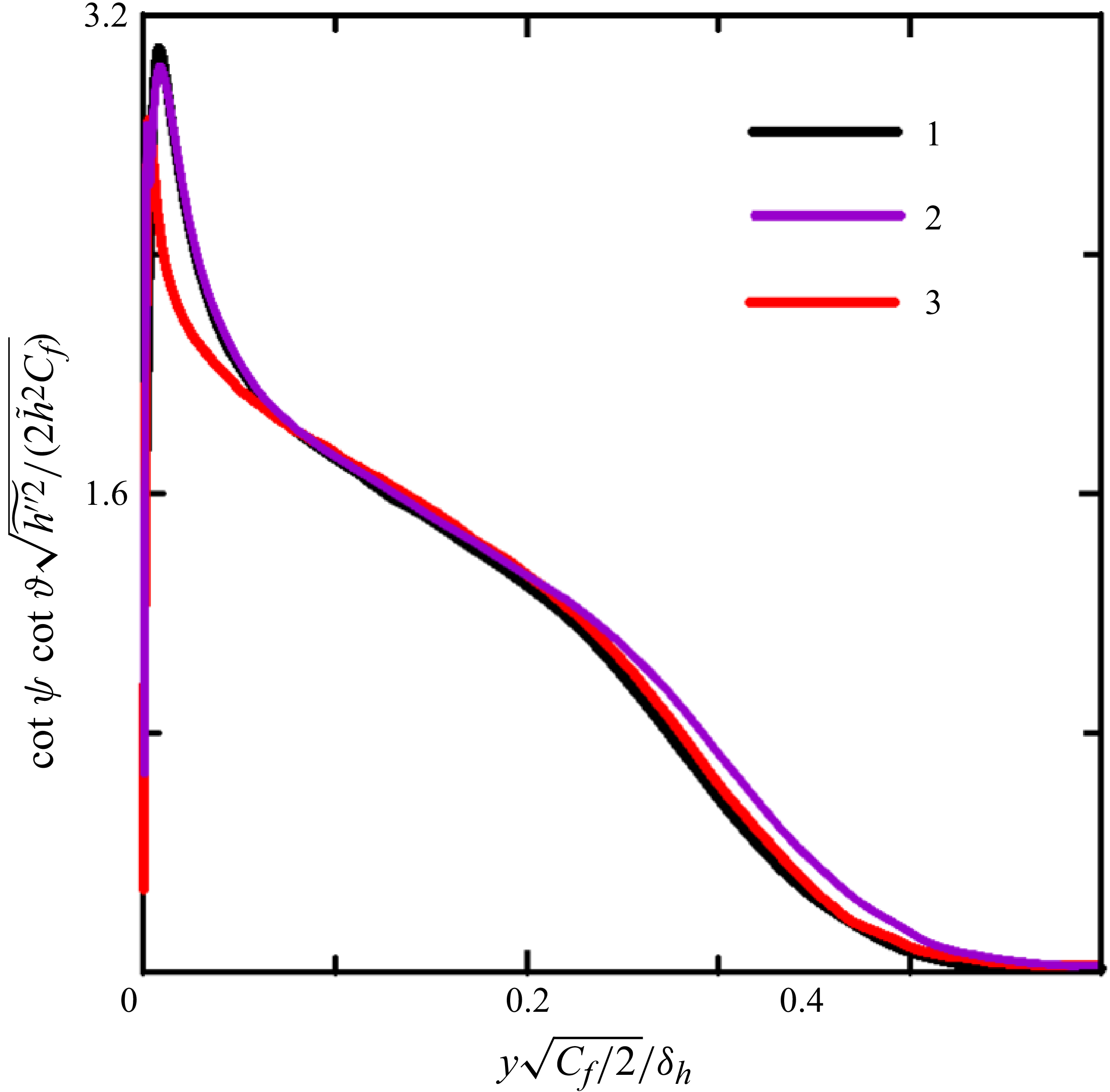
to close the boundary-layer equations (2.1), and also the expressions for the mean-square velocity and enthalpy fluctuations
 \begin{align} \widetilde {u^{\prime \prime 2}} &= \left ( y \frac {{\partial } \tilde u} {{\partial } y} \right )^2 U ({\textit{Re}},\, {\textit{Pe}},\, n,\, \eta ,\, \varPi _1,\, \varPi _2,\, \varGamma ), \end{align}
 \begin{align} \widetilde {h^{\prime \prime 2}} &= \left ( y \frac {{\partial } \tilde h}{{\partial } y} \right )^2 G ({\textit{Re}},\, {\textit{Pe}},\, n,\, \eta ,\, \varPi _1,\, \varPi _2,\, \varGamma ), \\{\textit{Re}} = \frac {\overline \rho y^2} {\tilde {\mu} } \frac {{\partial } \tilde u} {{\partial } y}, \!\!\quad {\textit{Re}} &= \textit{Pr} {\textit{Pe}}, \!\!\quad \eta = \frac y \delta , \!\!\quad \varPi _1 = \frac {y ({\partial } \tilde u / {\partial } y)^2}{{\partial } \tilde h / {\partial } y}, \!\!\quad \varPi _2 = \frac y {\tilde h} \frac {{\partial } \tilde h} {{\partial } y}, \!\!\quad \varGamma = \frac {\gamma \varPi _1 \varPi _2}{\gamma - 1}, \nonumber \end{align}
the existence of which was proved by Vigdorovich (Reference Vigdorovich2023a
). Here,
 $\delta$
is the boundary-layer thickness. These finite functional relationships are not based on partial hypotheses about the nature of turbulent exchange in the boundary layer or turbulence models. They are a direct consequence of the fact that the flow under consideration is completely determined by a finite set of given constant quantities, the governing parameters of the problem, which include the free-stream velocity
 $u_\infty$
, enthalpy
 $h_\infty$
, density
 $\rho _\infty$
and viscosity
 ${\mu} _\infty$
, the gas enthalpy
 $h_w$
at the wall, as well as the molecular Prandtl number, heat capacity ratio and exponent
 $n$
in the viscosity law (Vigdorovich Reference Vigdorovich2023a
). The universal functions
 $S$
,
 $H$
,
 $G$
and
 $U$
have the asymptotic expansions
 \begin{align} S &= S_0 ({\textit{Re}},\, \eta ) + \varPi _2 S_2 ({\textit{Re}},\, {\textit{Pe}},\, n/{\textit{Re}},\, \eta ) + O(\varPi _1 \varPi _2) + O\big(\varPi _2^2\big), \end{align}
 \begin{align} H &= H_0 ({\textit{Re}},\, {\textit{Pe}},\, \eta ) + \varPi _1 H_1 ({\textit{Re}},\, {\textit{Pe}},\, \eta ) + \varPi _2 H_2 ({\textit{Re}},\, {\textit{Pe}},\, n/{\textit{Re}},\, \eta ) \nonumber \\ &\quad + O(\varPi _1 \varPi _2) + O\big(\varPi _2^2\big), \end{align}
 \begin{align} G &= G_0 ({\textit{Re}},\, {\textit{Pe}},\, \eta ) + \varPi _1 G_1 ({\textit{Re}},\, {\textit{Pe}},\, \eta ) + \varPi _1^2 G_2 ({\textit{Re}},\, {\textit{Pe}},\, \eta )\nonumber \\ &\quad + \varPi _2 G_3 ({\textit{Re}},\, {\textit{Pe}},\, n/{\textit{Re}},\, \eta ) + O(\varPi _1 \varPi _2) + O\big(\varPi _2^2\big), \end{align}
 \begin{align} U &= U_0 ({\textit{Re}},\, \eta ) + \varPi _2 U_2 ({\textit{Re}},\, {\textit{Pe}},\, n/{\textit{Re}},\, \eta ) + O(\varPi _1 \varPi _2) + O\big(\varPi _2^2\big), \quad \varPi _2 \to 0. \end{align}
Since the parameter
 $\varPi _2$
expresses the relative enthalpy drop across the boundary layer and, thus, characterises flow compressibility, the first terms in expansions (2.4), the functions
 $S_0$
,
 $H_0$
,
 $G_0$
and
 $U_0$
, correspond to incompressible flow. The derivation of asymptotic representations (2.4) also dispenses with the involvement of physical hypotheses, but is based on the analysis of the general structure of the solution to the Navier–Stokes equations in the case of weakly compressible flow (Vigdorovich Reference Vigdorovich2023a
). The physical requirements for the closure relations are formulated only in terms of smoothness conditions for the universal functions. It is natural to consider
 $S_0$
,
 $S_2$
,
 $H_0$
,
 $H_1$
and
 $H_2$
as continuous and differentiable functions of their arguments, but it is sufficient to set weaker Hölder conditions
 \begin{align} S_0 ({\textit{Re}},\, \eta ) &= S_0 ({\textit{Re}},\, 0) + O(\eta ^{\alpha _1}), \quad \eta \to 0, \quad {\textit{Re}} = O(1), \nonumber \\ S_0 ({\textit{Re}},\, 0) &= S_0 (\infty ,\, 0) + O({\textit{Re}}^{-\alpha _2}), \quad {\textit{Re}} \to \infty , \nonumber \\ S_0 ({\textit{Re}},\, \eta ) &= S_0 (\infty ,\, \eta ) + O({\textit{Re}}^{-\alpha _2}), \quad {\textit{Re}} \to \infty , \quad 1/\eta = O(1), \nonumber \\ S_0 (\infty ,\, \eta ) &= S_0 (\infty ,\, 0) + O(\eta ^{\alpha _1}), \quad \eta \to 0, \quad \alpha _1, \alpha _2 \gt 0, \end{align}
and similar conditions for other universal functions. The conditions (2.5) are a mathematical formulation of the main physical assumption dating back to von Kármán (Reference von Kármán1930), according to which there are only two characteristic length scales in the flow under consideration: a viscous scale (that determines the viscous-sublayer thickness) and the boundary-layer thickness. At high Reynolds numbers, molecular viscosity and thermal conductivity are not significant outside the viscous sublayer, while the outer scale does not affect the flow in the near-wall region.
In what follows, we use the abbreviated notations
 \begin{align} \begin{split} S \left ( \infty ,\, \infty ,\, n,\, \eta ,\, \varPi _1,\, \varPi _2,\, \varGamma \right ) &= S_e \left ( \eta ,\, \varPi _1,\, \varPi _2,\, \varGamma \right )\!, \\ H \left ( \infty ,\, \infty ,\, n,\, \eta ,\, \varPi _1,\, \varPi _2,\, \varGamma \right ) &= H_e \left ( \eta ,\, \varPi _1,\, \varPi _2,\, \varGamma \right )\!, \end{split} \end{align}
which take into account that at
 ${\textit{Re}} \to \infty$
, the molecular viscosity and thermal conductivity and, hence, the value of
 $n$
, which specifies the viscosity law, are not significant outside the viscous sublayer.
3. Outer region of the boundary layer
3.1. Change of variables
Let us introduce the streamfunction
 $\psi _y = \overline \rho \tilde u$
and
 $\psi _x = - \overline \rho \tilde v$
and new variables by the formulas
 \begin{align} \psi = \rho _\infty u_\infty \delta \varPsi (\xi , \, \eta ), & \quad \tilde h = h_\infty + u_\infty ^2 \varPhi (\xi ,\, \eta ), \quad \overline \rho = \rho _\infty \omega (\xi ,\, \eta ), \nonumber \\ \xi = \ln {\textit{Re}}_\delta , &\quad {\textit{Re}}_\delta = \frac {\sqrt {\rho _\infty \rho _w}\, u_\infty \delta } {{\mu} _w}, \end{align}
where
 $\rho _w$
and
 ${\mu} _w$
are the averaged gas density and viscosity at the wall. Based on (3.1), we have
 \begin{align} {\partial }_x = \frac {\varLambda } {\delta } ( {\partial }_\xi - \eta {\partial }_\eta ), \quad {\partial }_y = \frac {{\partial }_\eta } \delta , \quad \varLambda (\xi ) = \frac {\textrm {d} \delta } {\textrm {d} x}, \end{align}
 \begin{align} \tilde u = u_\infty \omega ^{-1} \varPsi _\eta , \quad \tilde v = - u_\infty \varLambda \omega ^{-1} (\varPsi + \varPsi _\xi - \eta \varPsi _\eta ). \end{align}
The logarithm of the Reynolds number based on the boundary-layer thickness and the normalised distance from the wall are chosen as independent variables
 $\xi$
and
 $\eta$
. In addition to the dimensionless streamfunction
 $\varPsi (\xi ,\, \eta )$
and enthalpy
 $\varPhi (\xi ,\, \eta )$
, the third unknown function
 $\varLambda (\xi )$
– the growth rate of the boundary-layer thickness is introduced. From (2.1a
) and (2.1c
), for the functions
 $\varPsi$
,
 $\varPhi$
and
 $\varLambda$
, taking into account the closure relations (2.2), we obtain
 \begin{align} &\varLambda \big [ \varPsi _\eta \big(\omega ^{-1} \varPsi _\eta \big)_\xi - (\varPsi + \varPsi _\xi ) \big(\omega ^{-1} \varPsi _\eta \big)_\eta \big ] = \big \{ \omega \big [\eta \big(\omega ^{-1} \varPsi _\eta \big)_\eta \big ]^2 \!S_e (\eta ,\, \varPi _1,\, \varPi _2,\, \varGamma )\big \}_\eta, \end{align}
 \begin{align}&\qquad\quad \varLambda [\varPsi _\eta \varPhi _\xi - (\varPsi + \varPsi _\xi ) \varPhi _\eta ] = \big [ \omega \eta ^2 \varPhi _\eta \big(\omega ^{-1} \varPsi _\eta\big)_\eta H_e (\eta ,\, \varPi _1,\, \varPi _2,\, \varGamma ) \big ]_\eta \nonumber \\ &\qquad\qquad\qquad\qquad\qquad\qquad\qquad + \omega \eta ^2 \big[\big(\omega ^{-1} \varPsi _\eta\big)_\eta\big]^3 S_e (\eta ,\, \varPi _1,\, \varPi _2,\, \varGamma ), \end{align}
 \begin{align}&\qquad\qquad \omega ^{-1} = 1 + (\gamma - 1) M_\infty ^2 \varPhi , \quad \varPi _1 = \frac {\eta \big[\big(\omega ^{-1} \varPsi _\eta\big)_\eta\big]^2} {\varPhi _\eta }, \quad \varPi _2 = - \frac {{\partial } \ln \omega }{{\partial } \ln \eta }. \end{align}
Since (3.3) will be used only in the outer region of the boundary layer, the molecular viscosity and thermal conductivity terms are omitted, and the local Reynolds and Peclet numbers are set equal to infinity, which allows the notation (2.6) to be used.
Equations (3.3) are convenient for asymptotic analysis, since the boundary-layer thickness growth rate
 $\varLambda$
is a small quantity and the variable
 $\xi$
equal to the logarithm of the Reynolds number is a large quantity, which makes it possible to search for an asymptotic solution of the problem as
 $\xi \to \infty$
. The change of variables (3.1) and the equations for the desired functions (3.3) were first proposed by Vigdorovich (Reference Vigdorovich1993) for the boundary layer of an incompressible fluid.
3.2. Solution for the outer region
Let us consider the case of moderate free-stream Mach numbers
 $M_\infty = O(1)$
when, according to (3.3c
), the relative change in density across the boundary layer is of order one.
According to Vigdorovich (Reference Vigdorovich1993), the asymptotic expansions for the desired functions as
 $\xi \to \infty$
contain
 $\ln \xi$
in addition to inverse powers of
 $\xi$
. To simplify the form of the desired expansions and to avoid the appearance of logarithmic terms, we introduce a new independent variable
 $\zeta$
by the formula (Vigdorovich Reference Vigdorovich2017)
 \begin{align} \xi = \zeta + k \ln \zeta , \end{align}
where the coefficient
 $k$
will be chosen later. In the outer region of the boundary layer that is characterised by the condition
 $1/\eta = O(1)$
, we look for the solution of (3.3) in the form (Vigdorovich Reference Vigdorovich2017)
 \begin{align} \varLambda &= \lambda _1 \zeta ^{-1} + O(\zeta ^{-2}), \end{align}
 \begin{align} \frac {\tilde u}{u_\infty } &= \frac {\varPsi _\eta } \omega = 1 + \lambda _1 f_0 (\eta ) \zeta ^{-1} + O(\zeta ^{-2}), \end{align}
 \begin{align} \varPhi &= \lambda _2 \varphi _0 (\eta ) \zeta ^{-1} + O(\zeta ^{-2}), \quad \zeta \to \infty , \end{align}
where
 $\lambda _1$
and
 $\lambda _2$
are constant coefficients. For the dimensionless density, equalities (3.3c
) and (3.5c
) give
 \begin{align} \omega ^{-1} = 1 + (\gamma - 1) M_\infty ^2 \lambda _2 \varphi _0 (\eta ) \zeta ^{-1} + O(\zeta ^{-2}). \end{align}
Substituting (3.5b
)–(3.6) into (3.3d
) and (3.3e
), we obtain the estimates
 $\varPi _1 = O (\zeta ^{-1})$
and
 $\varPi _2 = O (\zeta ^{-1})$
, which on the basis of (2.6) and asymptotic representations (2.4a
) and (2.4b
) yield
 \begin{align} S_e (\eta ,\, \varPi _1,\, \varPi _2,\, \varGamma ) &= S_0 (\infty ,\, \eta ) + O (\zeta ^{-1}), \nonumber\\ H_e (\eta ,\, \varPi _1,\, \varPi _2,\, \varGamma ) &= H_0 (\infty ,\, \infty ,\, \eta ) + O (\zeta ^{-1}). \end{align}
By substituting the expansions (3.4)–(3.7) together with the equality
 $\varPsi = \eta + O (\zeta ^{-1})$
, which follows from (3.5b
) and (3.6), into (3.3) and taking the limit as
 $\zeta \to \infty$
with
 $1/\eta = O(1)$
, we obtain, for the functions
 $f_0$
and
 $\varphi _0$
, the ordinary differential equations
 \begin{align} \left [\big(\eta f^{\prime}_0\big)^2 S_0 (\infty ,\, \eta ) \right ]^{\prime} + \eta f^{\prime}_0 = 0; \quad f_0(\infty ) = 0, \end{align}
 \begin{align} \left [ \eta ^2 \varphi^{\prime}_{0} f^{\prime}_{0} H_0 (\infty ,\, \infty ,\, \eta ) \right ]^{\prime} + \eta \varphi^{\prime}_{0} = 0; \quad \varphi _0 (\infty ) = 0. \end{align}
The last term in (3.3b ) related to kinetic heating has a higher order of smallness and is not included in (3.8b ).
Equations (3.8) coincide completely with those obtained by Vigdorovich (Reference Vigdorovich2017) for the incompressible boundary layer. A non-zero solution to (3.8a ) has the form (Vigdorovich Reference Vigdorovich2017)
 \begin{align} f_0 (\eta ) = - \int \limits _\eta ^\infty \frac {{\textrm{d}}\eta _1} {2 \eta _1 \sqrt {S_0 (\infty ,\, \eta _1)}} \int \limits _{\eta _1}^\infty \frac {{\textrm{d}} \eta _2} {\sqrt {S_0 (\infty ,\, \eta _2)}} \end{align}
and is uniquely determined by the supplied boundary condition (3.8a ). From (3.9), given the smoothness conditions for the universal function (2.5), we obtain the asymptotic representation (Vigdorovich Reference Vigdorovich2017)
 \begin{align} f_0 (\eta ) &= \frac {I_0} \varkappa (\ln \eta + A_0 - \ln I_0) + O(\eta ^\alpha ), \quad \eta \to 0, \quad \alpha \gt 0, \end{align}
 \begin{align} I_0 &= \left (- \int _0^\infty f_0 \,\textrm {d} \eta \right )^{1/2} = \int \limits _0^\infty \frac {{\textrm{d}} \eta }{2 \sqrt {S_0 (\infty ,\, \eta )}}. \end{align}
Here,
 $\varkappa = \sqrt {S_0 (\infty ,\, 0)}$
and
 $A_0$
is some constant.
The boundary-layer thickness
 $\delta (x)$
introduced by us can be chosen with a significant degree of arbitrariness. Let us introduce a new transverse scale by the formula
 $\hat \delta = a \delta$
, where
 $a$
is a constant factor. Then
 $\hat \eta = a^{-1} \eta$
and
 $\hat \varLambda = a \varLambda$
. Hence, based on (3.5a
) and (3.5b
),
 $\hat f_0 = a^{-1} f_0$
. Consequently, based on (3.10b
),
 $\hat I_0 = a^{-1} I_0$
. It is now clear that the constant
 $A_0$
in (3.10a
) is introduced in such a way that it does not depend on
 $a$
, i.e. on the choice of the transverse scale
 $\delta$
.
The solution to (3.8b ) is
 \begin{align} \varphi _0 (\eta ) = C_2 \int \limits _\eta ^\infty \frac 1 \eta \textrm {d} \exp \left [- \int \limits _0^\eta \frac {\textrm {d} \eta } {\eta f^{\prime}_0 H_0 (\infty ,\, \infty ,\, \eta )} \right ] \end{align}
and is determined with accuracy to the constant
 \begin{align} C_2 = - \int \limits _0^\infty \varphi _0 \,\textrm {d} \eta \end{align}
(this equality is obtained by integrating (3.11) and taking the integral by parts), which can be chosen arbitrarily. Putting the additional condition
 \begin{align} \sigma \int \limits _0^\infty \varphi _0 \,{\textrm{d}} \eta = I_0, \quad \sigma = \frac {S_0 (\infty ,\, 0)}{H_0 (\infty ,\, \infty ,\, 0)}, \end{align}
where
 $\sigma$
is the turbulent Prandtl number in the logarithmic region (Vigdorovich Reference Vigdorovich2023b
), we obtain from (3.11) and the smoothness conditions (2.5) that the temperature profile has the logarithmic asymptotics at the wall
 \begin{align} \varphi _0 (\eta ) = - \frac 1 \varkappa (\ln \eta + E_0 - \ln I_0) + O(\eta ^\alpha ), \quad \eta \to 0, \quad \alpha \gt 0, \end{align}
where
 $E_0$
is a constant, which is also independent of the choice of the transverse scale
 $\delta$
.
The numerical values of the von Kármán constant
 $\varkappa$
, turbulent Prandtl number in the logarithmic region
 $\sigma$
and constants
 $A_0$
and
 $E_0$
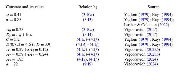
adopted in the present work are given in table 1.
Values of the empirical constants used.

Thus, the functions
 $f_0 (\eta )$
and
 $\varphi _0 (\eta )$
, specifying the dimensionless velocity and temperature defect profiles, can be taken from the solution for an incompressible fluid. The density variation in the outer region of the boundary layer is small and kinetic heating can be neglected.
3.3. Estimation of transverse pressure gradient
The Favre-averaged momentum equation in the
 $y$
direction has the form
 \begin{align} \frac {\partial } {{\partial } y} \big( \overline p + \overline \rho \tilde v^2 + \overline \rho \widetilde {v^{\prime \prime 2}} \big) = - \frac {\partial } {{\partial } x} \overline \rho \big( \tilde u \tilde v + \widetilde {u'' v''}\big). \end{align}
The molecular-viscosity terms in (3.15) are omitted. Integrating (3.15) over
 $y$
from zero to
 $\infty$
in view of the wall and free-stream conditions yields
 \begin{align} \overline p_w - p_\infty = \frac {\partial } {{\partial } x} \int _0^\infty \overline \rho \big( \tilde u \tilde v + \widetilde {u'' v''}\big) \textrm {d} y. \end{align}
Equality (3.2e
) and the expansions (3.5a
) and (3.5b
) imply that the dimensionless transverse velocity component is of order
 $\zeta ^{-2}$
, and the dimensionless shear stress is of the same order by virtue of (2.2a
) and (3.5b
). According to (3.2a
), differentiating by
 $x$
raises the order of the right-hand side of (3.16) by two more units. Thus, for the dimensionless pressure difference, we obtain the estimate
 \begin{align} \frac {\overline p_w - p_\infty }{\rho _\infty u_\infty ^2} = O (\zeta ^{-4}), \end{align}
which is enough to put
 $\overline p_w = p_\infty$
wherever necessary in further calculations.
4. Crocco integral in the logarithmic sublayer and laws of the wall for velocity and temperature
Vigdorovich (Reference Vigdorovich2023b , Reference Vigdorovich2024) obtained asymptotic representations for the velocity and temperature profiles in the logarithmic region of the boundary layer, which are formulated as a functional relationship between temperature and velocity (the Crocco integral) and laws of the wall for velocity and temperature:
 \begin{align} &\qquad\qquad h_w = \tilde h + \sigma \frac {\tilde u^2} 2 + \sigma \frac {\tilde u q_w}{\tau _w} +\frac {\varepsilon _* h_w P (\phi ,\, \phi _w)}{\cos ^2 \phi _w} + O\big(\varepsilon _*^2\big), \end{align}
 \begin{align} & \frac {\phi - \phi _w}{\varepsilon _*} + Q_1 (\phi ,\, \phi _w) + O(\varepsilon _*) = \frac 1 \varkappa \ln y_+ + D_1 (\textit{Pr},\, n,\, Q_+) + O\big(y_+^{-\alpha }\big), \end{align}
 \begin{align} &\quad \frac {\psi - \phi _w}{\varepsilon _*} + R (\psi ,\, \phi _w) + O (\varepsilon _*) = \frac 1 \varkappa \ln y_+ + D_1 (\textit{Pr},\, n,\, Q_+) + O\big(y_+^{-\alpha }\big), \\\varepsilon _* & = \sqrt {\frac {\sigma \tau _w}{2 h_w \rho _w}}, \quad y_+ = \frac {y \sqrt {\rho _w \tau _w}}{{\mu} _w};\quad \phi _w \leqslant \phi \lt \frac \pi 2, \quad y_+ \to \infty , \quad \alpha \gt 0, \nonumber \end{align}
 \begin{align} &\quad P(\phi ,\,\phi _w) = 2 A_1 (\phi - \phi _w) + A_2 \sin 2 \phi + [D (\textit{Pr}) - C - A_2] \sin 2 \phi _w, \end{align}
 \begin{align} &\quad Q_1 (\phi ,\, \phi _w) = A_1 (\phi - \phi _w) \tan \phi + A_3 \ln \frac {\cos \phi } {\cos \phi _w} \nonumber \\ &\qquad\qquad\qquad - A_2 \frac {\sin \phi _w \sin (\phi - \phi _w)} {\cos \phi } + [D (\textit{Pr}) - C] \frac {\cos \phi _w \cos (\phi - \phi _w)}{\cos \phi }, \end{align}
 \begin{align} &\quad R (\psi ,\, \phi _w) = -A_1 (\psi - \phi _w) \cot \psi + A_3 \ln \frac {\cos \psi } {\cos \phi _w} \nonumber\\ &\qquad\qquad\qquad + [D (\textit{Pr}) - C - A_2] \frac {\cos \phi _w \sin (\psi - \phi _w)} {\sin \psi }.\end{align}
The Crocco integral (4.1a ) and the laws of the wall for velocity (4.1b ) and temperature (4.1c ) are written in the similarity variables
 \begin{align} \phi &= \arcsin \frac {\sqrt \sigma (\tilde u + q_w/\tau _w)} {\sqrt {2 h_w + \sigma (q_w/\tau _w)^2}}, \end{align}
 \begin{align} \psi &= \arccos \frac {\sqrt {2 \tilde h}}{\sqrt {2 h_w + \sigma (q_w/\tau _w)^2}} = \arccos \left (\!\cos \phi _w \sqrt {\tilde h/h_w} \right )\!, \end{align}
where
 $\tau _w$
and
 $q_w$
are the shear stress and heat flux at the wall, respectively, and
 \begin{align} \phi _w = \arctan \frac {\sqrt \sigma q_w}{\tau _w \sqrt {2 h_w}} \end{align}
is the value of the variable
 $\phi$
at
 $\tilde u = 0$
. In addition to the von Kármán constant
 $\varkappa$
, turbulent Prandtl number in the logarithmic region
 $\sigma$
and quantities
 $C$
and
 $D (\textit{Pr})$
, which are included in the logarithmic laws (laws of the wall) for velocity and temperature in an incompressible fluid (Vigdorovich Reference Vigdorovich2017, Reference Vigdorovich2023b
), relations (4.1) contain three new universal constants
 $A_1$
,
 $A_2$
and
 $A_3$
determined in (Vigdorovich Reference Vigdorovich2023b
, Reference Vigdorovich2024) by comparison with direct numerical simulation (DNS) data. The numerical values of these quantities are given in table 1. The empirical function
 $D_1 (\textit{Pr},\, n,\, Q_+)$
depends on the molecular Prandtl number, the law of viscosity and heat conductivity, which in this case is specified by the exponent
 $n$
, and the dimensionless heat flux
 \begin{align} Q_+ = \frac {q_w}{h_w \sqrt {\rho _w \tau _w}}. \end{align}
The equality
 $D_1 (\textit{Pr},\, n,\, 0) = D (\textit{Pr})$
holds. The Crocco integral and laws of the wall for velocity and temperature are obtained by Vigdorovich (Reference Vigdorovich2023b
, Reference Vigdorovich2024) as asymptotic expansions in the small parameter
 $\varepsilon _*$
, which is proportional to the Mach number formed with the friction velocity and the speed of sound at the wall. By introducing the skin-friction coefficient
 $C_{\!f} = 2 \tau _w/\rho _\infty u_\infty ^2$
and neglecting, according to the result formulated in § 3.3, the pressure drop across the layer, we obtain
 \begin{align} \varepsilon _* = \tan \vartheta \sqrt {\frac {1}{2} C_{\!f}}, \quad \tan \vartheta = \sqrt {\frac {\sigma u_\infty ^2}{2 h_\infty }} = M_\infty \sqrt {\frac {1}{2} \sigma (\gamma - 1)}. \end{align}
As shown by Vigdorovich (Reference Vigdorovich2023b ), in zeroth-order approximation in the small parameter, the Crocco integral (4.1a ) yields the well-known Walz (Reference Walz1966) equation, while the leading term of the expansion on the left-hand side of (4.1b ) is the Van Driest (Reference Van Driest1951) formula in the form given, e.g. by Wilcox (Reference Wilcox2006).
The range of applicability of the law of the wall for velocity (4.1b
) is the logarithmic sublayer – an intermediate region located between the outer region and the viscous sublayer at the wall. The same applies to the law of the wall for temperature (4.1c
) in the cases of a heated and adiabatic plate. In the boundary layer on a cooled plate, the temperature behaves non-monotonically across the layer, and relation (4.1c
) is valid only in the upper part of the logarithmic sublayer above the temperature maximum point. Since the Crocco integral (4.1a
) can be written as
 $\cos ^2 \psi = \cos ^2 \phi + O(\varepsilon _*)$
, in the region of a one-to-one relationship between velocity and temperature the equality holds
 \begin{align} \psi = \phi + O(\varepsilon _*), \end{align}
which we will use further.
5. Matching of solutions for the outer region and logarithmic sublayer
The relationships obtained in the logarithmic region, the Crocco integral and laws of the wall for velocity and temperature, contain as a parameter an unknown quantity – the wall shear stress or skin-friction coefficient. The expansions for the velocity and temperature profiles in the outer region (3.5b
) and (3.5c
) contain the coefficients
 $\lambda _1$
and
 $\lambda _2$
to be determined. These three quantities will be determined as a result of asymptotic matching of the solutions for the two regions.
5.1. Matching on the basis of the law of the wall for velocity
The law of the wall for the velocity profile (4.1b
) is an asymptotic expansion of the solution to the problem in the near-wall region as
 $y_+ \to \infty$
. Following the matching procedure (Van Dyke Reference Van Dyke1975), let us rewrite it in outer variables. The relation between the variables reads
 \begin{align} y_+ = {\textit{Re}}_\tau \eta , \quad {\textit{Re}}_\tau = \frac {\delta \sqrt {\rho _w \tau _w}}{{\mu} _w} = {\textit{Re}}_\delta \sqrt {\frac {1}{2} C_{\!f}}. \end{align}
Here, the definition of
 ${\textit{Re}}_\delta$
(3.1) is taken into account. According to (3.5b
) in the outer region
 \begin{align} \tilde u = u_\infty + u_\infty \lambda _1 f_0 (\eta ) \zeta ^{-1} + O(\zeta ^{-2}). \end{align}
Let us substitute (5.2) into the left-hand side of equality (4.1b
) and under the condition
 $1/\eta = O(1)$
, when
 $f_0 (\eta ) = O(1)$
, expand it in the small parameter
 $\zeta ^{-1}$
. The result is
 \begin{align} &\frac {\phi _\infty - \phi _w}{\tan \vartheta \sqrt {\frac {1}{2} C_{\!f}}} + \frac {u_\infty \phi ' (u_\infty ) \lambda _1 f_0 (\eta )} {\zeta \tan \vartheta \sqrt {\frac {1}{2} C_{\!f}}} + Q_1 (\phi _\infty ,\, \phi _w) + O(\zeta ^{-1}) + O \big(\sqrt {C_{\!f}}\big) \nonumber \\ &\quad = \frac 1 \varkappa \ln (\eta {\textit{Re}}_\tau ) + D_1 (\textit{Pr},\, n,\, Q_+) + O\big({\textit{Re}}_\tau ^{-\alpha }\big). \end{align}
Here we used (4.5a
), and
 $\phi _\infty = \phi (u_\infty )$
is the value of the variable
 $\phi$
(4.2a
) at the outer boundary of the boundary layer. From (4.2) we have
 \begin{align} \phi '(\tilde u) = \frac {\cos \psi }{\cos \phi } \sqrt {\frac \sigma {2 \tilde h}}, \end{align}
which based on (4.5b ) and (4.6) allows us to write
 \begin{align} u_\infty \phi ' (u_\infty ) = \tan \vartheta + O \big(\sqrt {C_{\!f}}\big). \end{align}
Let us now take in (5.3) the limit as
 $\eta \to 0$
. For this purpose, we replace the function
 $f_0 (\eta )$
by its asymptotic expansion (3.10a
). As a result, in view of (5.5), we obtain the matching condition (Van Dyke Reference Van Dyke1975)
 \begin{align} &\frac {\phi _\infty - \phi _w} {\tan \vartheta \sqrt {\frac {1}{2} C_{\!f}}} + \frac {I_0 \lambda _1}{\varkappa \zeta \sqrt {\frac {1}{2} C_{\!f}}} (\ln \eta + A_0 - \ln I_0) + Q_1 (\phi _\infty ,\, \phi _w) + O(\zeta ^{-1}) + O \big(\sqrt {C_{\!f}}\big) \nonumber \\ &\quad = \frac 1 \varkappa \ln (\eta {\textit{Re}}_\tau ) + D_1 (\textit{Pr},\, n,\, Q_+). \end{align}
Equating in this equality the coefficients at
 $\ln \eta$
, we have
 \begin{align} \sqrt {\frac {1}{2} C_{\!f}} = \frac {I_0 \lambda _1} \zeta + O(\zeta ^{-2}). \end{align}
The second relation that follows from (5.6) is the friction law
 \begin{align} \ln (I_0 {\textit{Re}}_\tau ) = \frac {\varkappa (\phi _\infty - \phi _w)} {\tan \vartheta \sqrt {\frac {1}{2} C_{\!f}}} + \varkappa [Q_1 (\phi _\infty ,\, \phi _w) - D_1 (\textit{Pr},\, n,\, Q_+)] + A_0 + O \big(\sqrt {C_{\!f}}\big), \end{align}
i.e. a relationship between the skin-friction coefficient and Reynolds number. It is taken into account here that according to (5.7) and (4.5a
),
 $\sqrt {C_{\!f}} = O(\zeta ^{-1})$
.
Based on (5.1), (3.1), (3.4) and (5.7),
 \begin{align} \ln {\textit{Re}}_\tau = \zeta + k \ln \zeta + \ln \sqrt {\frac {1}{2} C_{\!f}} = \zeta + (k - 1) \ln \zeta + O(1). \end{align}
On the other hand, substitution of (5.7) into (5.8) yields
 \begin{align} \ln {\textit{Re}}_\tau = \frac {\varkappa (\phi _\infty - \phi _w) \zeta }{I_0 \lambda _1 \tan \vartheta } + O(1). \end{align}
From a comparison of (5.9) and (5.10), we obtain
 $k = 1$
and
 \begin{align} \lambda _1 = \frac {\varkappa (\phi _\infty - \phi _w)}{I_0 \tan \vartheta }. \end{align}
5.2. Matching on the basis of the Crocco integral
Let us now perform the matching based on the Crocco integral (4.1a ). On the basis of (3.1) and (3.5c ) in the outer region
 \begin{align} \tilde h = h_\infty + u_\infty ^2 \lambda _2 \varphi _0 (\eta ) \zeta ^{-1} + O(\zeta ^{-2}). \end{align}
Substitution of (5.2) and (5.12) into (4.1a
) and expanding in the small parameter
 $\zeta ^{-1}$
under the condition
 $1/\eta = O(1)$
, when
 $f_0 (\eta ) = O(1)$
and
 $\varphi _0 (\eta ) = O(1)$
, yield
 \begin{align} h_w - h_\infty - \frac {\sigma u_\infty ^2} 2 - \frac {\sigma u_\infty q_w}{\tau _w} &= \frac {u_\infty ^2 \lambda _2} \zeta \varphi _0 (\eta ) + \sigma u_\infty \left ( u_\infty + \frac {q_w}{\tau _w} \right ) \frac {\lambda _1} \zeta f_0(\eta ) \nonumber \\ &\quad + \frac {h_w \tan \vartheta P (\phi _\infty ,\, \phi _w)}{\cos ^2 \phi _w} \sqrt {\frac {1}{2} C_{\!f}} + O(C_{\!f}). \end{align}
Here, we also used (4.5a
) and took into account that
 $\sqrt {C_{\!f}} = O(\zeta ^{-1})$
. Taking in this equality the limit as
 $\eta \to 0$
, i.e. replacing the functions
 $f_0$
and
 $\varphi _0$
by their asymptotic expansions (3.10a
) and (3.14), gives the matching condition (Van Dyke Reference Van Dyke1975)
 \begin{align} h_w - h_\infty - \frac {\sigma u_\infty ^2} 2 - \frac {\sigma u_\infty q_w}{\tau _w} &= \frac {u_\infty ^2 \lambda _2}{\varkappa \zeta } (\ln \eta + E_0 - \ln I_0) \nonumber \\ &\quad + \sigma u_\infty \left ( u_\infty + \frac {q_w}{\tau _w} \right ) \frac {I_0 \lambda _1}{\varkappa \zeta } (\ln \eta + A_0 - \ln I_0) \nonumber \\ &\quad + \frac {h_w \tan \vartheta P (\phi _\infty ,\, \phi _w)}{\cos ^2 \phi _w} \sqrt {\frac {1}{2} C_{\!f}} + O(C_{\!f}). \end{align}
By equating the coefficients at
 $\ln \eta$
, in view of (5.7), we have
 \begin{align} \frac {\lambda _2} \zeta = \sigma \left ( 1 + \frac {q_w}{u_\infty \tau _w} \right ) \sqrt {\frac {1}{2} C_{\!f}} + O(C_{\!f}). \end{align}
The second relation, which follows from (5.14),
 \begin{align}& h_w - h_\infty - \frac {\sigma u_\infty ^2} 2 - \frac {\sigma u_\infty q_w}{\tau _w} \nonumber\\ &\quad= \sqrt {\frac {1}{2} C_{\!f}} \left [ \frac {\sigma u_\infty } \varkappa \left ( u_\infty + \frac {q_w}{\tau _w} \right ) (A_0 - E_0) + \frac {h_w \tan \vartheta P (\phi _\infty ,\, \phi _w)}{\cos ^2 \phi _w} \right ] + O(C_{\!f}), \end{align}
will allow us to calculate the recovery and Reynolds-analogy factors.
5.3. Matching on the basis of the law of the wall for temperature
Substituting (5.12) into (4.2b ), we get
 \begin{align} \psi = \psi _\infty + \psi ' (h_\infty ) u_\infty ^2 \lambda _2 \varphi _0 (\eta ) \zeta ^{-1} + O (\zeta ^{-2}). \end{align}
Here,
 $\psi _\infty = \psi (h_\infty )$
is the value of the variable
 $\psi$
(4.2b
) at the outer boundary of the boundary layer. Since based on (4.2b
),
 \begin{align} \psi '(\tilde h) = - \frac {\cot \psi }{2 \tilde h}, \end{align}
we obtain
 \begin{align} \psi = \psi _\infty - \frac 12 (\gamma - 1) M_\infty ^2 \cot \psi _\infty \lambda _2 \varphi _0 (\eta ) \zeta ^{-1} + O (\zeta ^{-2}), \end{align}
which after substitution into (4.1c
) and expanding in terms of the small parameter
 $\zeta ^{-1}$
yields
 \begin{align} \frac {\psi _\infty - \phi _w} {\tan \vartheta \sqrt {\frac {1}{2} C_{\!f}}} &- \frac {(\gamma - 1) M_\infty ^2 \cot \psi _\infty \lambda _2 \varphi _0 (\eta )} {2 \zeta \tan \vartheta \sqrt {\frac {1}{2} C_{\!f}}} + R (\psi _\infty ,\, \phi _w) + O \big(\sqrt {C_{\!f}}\big) \nonumber \\ &= \frac 1 \varkappa \ln ({\textit{Re}}_\tau \eta ) + D_1 (\textit{Pr},\, n,\, Q_+) + O\big({\textit{Re}}_\tau ^{-\alpha }\big). \end{align}
We obtain the matching condition (Van Dyke Reference Van Dyke1975) by replacing the function
 $\varphi _0 (\eta )$
in this equality by its asymptotic expansion (3.14):
 \begin{align} \frac {\psi _\infty - \phi _w}{\tan \vartheta \sqrt {\frac {1}{2} C_{\!f}}} &+ \frac {\cot \psi _\infty \tan \vartheta \lambda _2} {\sigma \varkappa \zeta \sqrt {\frac {1}{2} C_{\!f}}} (\ln \eta + E_0 - \ln I_0) + R (\psi _\infty ,\, \phi _w) + O \big(\sqrt {C_{\!f}}\big) \nonumber \\ &= \frac 1 \varkappa \ln ({\textit{Re}}_\tau \eta ) + D_1 (\textit{Pr},\, n,\, Q_+). \end{align}
Here we have taken into account equality (4.5b
). Now, equating in (5.21) the coefficients at
 $\ln \eta$
, we have
 \begin{align} \frac {\lambda _2} \zeta = \frac {\sigma \tan \psi _\infty }{\tan \vartheta } \sqrt {\frac {1}{2} C_{\!f}} + O(C_{\!f}). \end{align}
Using (4.6) and then (4.2) with the accuracy of
 $O(\sqrt {C_{\!f}})$
yields
 \begin{align} \frac {\tan \psi _\infty }{\tan \vartheta } = \frac {\sin \phi _\infty }{\cos \psi _\infty \tan \vartheta } = \frac {\sqrt \sigma (u_\infty + q_w/\tau _w)}{\tan \vartheta \sqrt {2 h_\infty }}. \end{align}
Hence, given (4.5b
), we can conclude that the expression for
 $\lambda _2$
(5.22) coincides with (5.15).
The second relation, which follows from the matching condition (5.21), is another formulation of the friction law
 \begin{align} \ln (I_0 {\textit{Re}}_\tau ) = \frac {\varkappa (\psi _\infty - \phi _w)} {\tan \vartheta \sqrt {\frac {1}{2} C_{\!f}}} + \varkappa [R (\psi _\infty ,\, \phi _w) - D_1 (\textit{Pr},\, n,\, Q_+)] + E_0 + O \big(\sqrt {C_{\!f}}\big). \end{align}
6. Recovery and Reynolds-analogy factors
6.1. Recovery factor
In the case of an adiabatic plate, when
 $q_w = 0$
,
 $\phi _w = 0$
and
 $h_w = h_r$
, (5.16) takes the form
 \begin{align} u_\infty ^2 (r - \sigma ) = \sqrt {2 C_{\!f}}\, \left [ \frac {\sigma u_\infty ^2} \varkappa (A_0 - E_0) + h_r \tan \vartheta P (\phi _\infty ,\, 0) \right ] + O(C_{\!f}). \end{align}
At zero heat flux, (4.2a ) implies that
 \begin{align} \sin ^2 \phi _\infty = \frac {\sigma u_\infty ^2}{2 h_r}, \end{align}
which allows us to write (6.1) as
 \begin{align} \frac r \sigma = 1 + \sqrt {\frac {1}{2} C_{\!f}} \left [ \frac 2 \varkappa (A_0 - E_0) + \frac {\tan \vartheta P (\phi _\infty ,\, 0)} {\sin ^2 \phi _\infty } \right ] + O(C_{\!f}). \end{align}
This equality confirms the estimate given by Van Driest (Reference Van Driest1956, Reference Van Driest1959) for the recovery factor
 $r = \sigma + O (\sqrt {C_{\!f}})$
, using which, based on (4.5b
), we write (6.2) in the form
 \begin{align} \sin ^2 \phi _\infty = \frac {\sigma u_\infty ^2}{2 h_\infty + r u_\infty ^2} = \sin ^2 \vartheta \left [ 1 + O \big(\sqrt {C_{\!f}}\big) \right ] \end{align}
or
 $\phi _\infty = \vartheta + O(\sqrt {C_{\!f}})$
, which in view of the expression (4.1d
) for the function
 $P(\phi _\infty ,\, 0)$
, allows us to finally write the recovery factor as
 \begin{align} \frac r \sigma = 1 + \sqrt {2 C_{\!f}} \left ( \frac {A_0 - E_0} \varkappa + A_2 + \frac {2 A_1 \vartheta } {\sin 2 \vartheta } \right ) + O(C_{\!f}). \end{align}
Thus, just like Van Driest (Reference Van Driest1956, Reference Van Driest1959), we have obtained the recovery factor for the boundary layer on a flat plate in the form of an asymptotic expansion in the small parameter – the root of the skin-friction coefficient. The leading term of the expansion is the turbulent Prandtl number in the logarithmic region
 $\sigma$
, and the coefficient of the small parameter, in view of the expression for
 $\vartheta$
(4.5b
), is a function of the Mach number and heat capacity ratio. In addition, relation (6.5) contains five more universal constants, three of which --
 $\varkappa$
,
 $A_0$
and
 $E_0$
-- are known for the incompressible boundary layer, while
 $A_1$
and
 $A_2$
enter the Crocco integral for a compressible gas (Vigdorovich Reference Vigdorovich2023b
).
Since according to (4.5b
),
 $\vartheta \to \pi /2$
as
 $M_\infty \to \infty$
, the expression (6.5) has a singularity at
 $M_\infty = \infty$
and, hence, is valid only at moderate free-stream Mach numbers. On the other hand, the limit at
 $M_\infty = 0$
exists and is equal to
 \begin{align} \frac r \sigma = 1 + \sqrt {2 C_{\!f}} \left ( \frac {A_0 - E_0} \varkappa + A_1 + A_2 \right ) + O(C_{\!f}). \end{align}
This equality can be compared with the expression obtained by Rotta (Reference Rotta1964) for an incompressible fluid,
 $r = \sigma + B_0 \sqrt {{C_f /2}} + O(C_{\!f})$
, which differs only in the value of the coefficient
 $B_0 \approx 1$
. It is about half of the corresponding coefficient in (6.6).
Note that according to (6.5), the recovery factor with the accuracy of
 $O(C_{\!f})$
is independent of the molecular Prandtl number. Furthermore, this conclusion is supported by the expressions obtained by Van Driest (Reference Van Driest1956, Reference Van Driest1959) and Rotta (Reference Rotta1964).
6.2. Reynolds-analogy factor
By introducing the Stanton number
 $St = q_w /\rho _\infty u_\infty (h_w - h_r)$
and the Reynolds-analogy factor
 $\alpha = 2 St/C_{\!f}$
, we can write
 \begin{align} \frac {u_\infty q_w}{\tau _w} = \alpha (h_w - h_r), \end{align}
which after substitution into (5.16) gives
 \begin{align} & (1 - \sigma \alpha )(h_w - h_r) + (r - \sigma ) \frac {u_\infty ^2} 2 \nonumber \\ &\quad = \sqrt {\frac {1}{2} C_{\!f}} \left \{ \frac \sigma \varkappa \left [ u_\infty ^2 + \alpha (h_w - h_r) \right ] (A_0 - E_0) + \frac {h_w \tan \vartheta P (\phi _\infty ,\, \phi _w)}{\cos ^2 \phi _w} \right \} + O(C_{\!f}). \end{align}
The second term on the left-hand side of (6.8), in view of the expression for the recovery factor (6.5), has the form
 \begin{align} (r - \sigma ) \frac {u_\infty ^2} 2 = \sigma u_\infty ^2 \sqrt {\frac {1}{2} C_{\!f}} \left ( \frac {A_0 - E_0} \varkappa + A_2 + \frac {2 A_1 \vartheta } {\sin 2 \vartheta } \right ) + O(C_{\!f}), \end{align}
which after substitution into (6.8) yields
 \begin{align} (1 - \sigma \alpha )(h_w - h_r) &= \sqrt {\frac {1}{2} C_{\!f}} \left [ \frac {\sigma \alpha } \varkappa (h_w - h_r)(A_0 - E_0) - \sigma u_\infty ^2 \left ( A_2 + \frac {2 A_1 \vartheta } {\sin 2 \vartheta } \right ) \right . \nonumber \\ &\quad +\left . \, \frac {h_w \tan \vartheta P (\phi _\infty ,\, \phi _w)}{\cos ^2 \phi _w} \right ] + O(C_{\!f}). \end{align}
In view of the expression (4.1d
) for the function
 $P(\phi _\infty ,\, \phi _w)$
, the last term on the right-hand side of (6.10) is
 \begin{align} \frac {h_w \tan \vartheta P (\phi _\infty ,\, \phi _w)}{(h_w - h_r) \cos ^2 \phi _w} = \frac {h_w \tan \vartheta }{(h_w - h_r)} \left \{ \frac {2 A_1 (\phi _\infty - \phi _w)}{\cos ^2 \phi _w} \right . \nonumber \\ \left . + \frac {A_2 \sin 2 \phi _\infty }{\cos ^2 \phi _w} + 2 [D (\textit{Pr}) - C - A_2] \tan \phi _w \right \}\!. \end{align}
Equality (6.10) implies the estimate given by Van Driest (Reference Van Driest1956, Reference Van Driest1959) for the Reynolds-analogy factor
 $\alpha = 1/\sigma + O (\sqrt {C_{\!f}})$
, by using which along with (4.2), (4.3), (4.5b
), (4.6) and (6.7), we have with the accuracy of
 $O(\sqrt {C_{\!f}})$
:
 \begin{align} \frac {h_w \tan \vartheta \sin 2 \phi _\infty }{(h_w - h_r) \cos ^2 \phi _w} = 1 + \frac {\sigma u_\infty ^2}{h_w - h_r}, \quad \frac {2 h_w \tan \vartheta \tan \phi _w}{(h_w - h_r)} = \sqrt {\frac {h_w}{h_\infty }}. \end{align}
Substitution of (6.11) and (6.12) into (6.10) yields
 \begin{align} \sigma \alpha = 1 & + \sqrt {\frac {1}{2} C_{\!f}} \left [ \frac {E_0 - A_0} \varkappa - A_2 + [C + A_2 - D (\textit{Pr})] \sqrt {\frac {h_w}{h_\infty }} \right . \nonumber \\ & \left . +\, \frac {2 A_1}{h_w - h_r} \left ( \frac {\sigma u_\infty ^2 \vartheta }{\sin 2 \vartheta } - \frac {(\phi _\infty - \phi _w) h_w \tan \vartheta }{\cos ^2 \phi _w} \right ) \right ] + O(C_{\!f}). \end{align}
Replacing in (6.7)
 $r$
and
 $\alpha$
by
 $\sigma$
and
 $1/\sigma$
, respectively, we get
 \begin{align} \frac {u_\infty q_w}{\tau _w} = \left ( \frac {h_w - h_\infty } \sigma - \frac {u_\infty ^2} 2 \right ) \left [1 + O \big(\sqrt {C_{\!f}}\big) \right ]\!. \end{align}
The quantities
 $\phi _\infty$
and
 $\phi _w$
on the right-hand side of (6.13) as well as
 $\psi _\infty$
can be calculated to the accuracy of
 $O(\sqrt {C_{\!f}})$
using (4.2), (4.3) and (6.14) in terms of the free-stream parameters and wall enthalpy. Denoting the corresponding quantities by
 $\phi ^{\prime}_\infty$
,
 $\psi ^{\prime}_\infty$
and
 $\phi ^{\prime}_w$
, we have
 \begin{align} \psi ^{\prime}_\infty &= \phi ^{\prime}_\infty = \arctan \left [ \frac {(2 + \sigma Ec) \tan \vartheta }{2 \sigma Ec} \right ]\!, \end{align}
 \begin{align} \phi ^{\prime}_w &= \arctan \left [ \frac {(2 - \sigma Ec) \tan \vartheta }{2 \sigma Ec} \sqrt {\frac {h_\infty }{h_w}} \right ]\!, \quad Ec = \frac {u_\infty ^2}{h_w - h_\infty } = \frac {(\gamma - 1) M_\infty ^2}{h_w/h_\infty - 1}, \\[9pt] \nonumber \end{align}
where
 $Ec$
is the Eckert number characterising gas kinetic heating. Then, we finally obtain
 \begin{align} \sigma \alpha = 1 + \sqrt {\frac {1}{2} C_{\!f}} \left [ \frac {E_0 - A_0} \varkappa - A_2 + [C + A_2 - D (\textit{Pr})] \sqrt {\frac {h_w}{h_\infty }} \right . \nonumber\\ \left . + A_1 \cot \phi ^{\prime}_w \left (\frac \vartheta {\cos ^2 \vartheta } - \frac {\psi ^{\prime}_\infty - \phi ^{\prime}_w} {\cos ^2 \psi ^{\prime}_\infty } \right ) \sqrt {\frac {h_\infty }{h_w}} \right ] + O(C_{\!f}). \end{align}
Formula (6.16) specifies the Reynolds-analogy factor in the form of an asymptotic expansion in the small parameter
 $\sqrt {C_{\!f}}$
, the leading term of which is the reciprocal of the turbulent Prandtl number, which coincides in structure with the expression obtained by Van Driest (Reference Van Driest1956, Reference Van Driest1959). Compared with the recovery factor, the number of parameters on which the Reynolds-analogy factor depends is two more due to the enthalpy ratio
 $h_w/h_\infty$
and the molecular Prandtl number. The latter quantity enters (6.16) via the function
 $D (\textit{Pr})$
, which is known from the logarithmic law for temperature in an incompressible fluid (Vigdorovich Reference Vigdorovich2017, Reference Vigdorovich2023b
). Equality (6.16) also includes the constant
 $C$
from the logarithmic law for the velocity profile in an incompressible fluid (Vigdorovich Reference Vigdorovich2017, Reference Vigdorovich2023b
).
Since when
 $M_\infty \to \infty$
,
 $\vartheta \to \pi /2$
according to (4.5b
) and
 $\phi ^{\prime}_\infty \to \pi /2$
according to (6.15a
), the expression (6.16) has a singularity at
 $M_\infty = \infty$
and, therefore, like the expression (6.5) for the recovery factor, is valid only at moderate free-stream Mach numbers. In the case of incompressible flow taking in (6.16) the limit as
 $\vartheta \to 0$
and
 $h_w/h_\infty \to 1$
, we have the expression
 \begin{align} \sigma \alpha = 1 + \sqrt {\frac {1}{2} C_{\!f}} \left [ \frac {E_0 - A_0} \varkappa + C - D (\textit{Pr}) \right ] + O(C_{\!f}), \end{align}
which was obtained by Vigdorovich (Reference Vigdorovich2017) for the incompressible boundary layer.
The case of an adiabatic plate (
 $h_w = h_r$
) corresponds to the limit as
 $Ec \to 2/\sigma$
, for which from (6.15) we have
 \begin{align} \phi ^{\prime}_\infty = \vartheta + \frac {2 - \sigma Ec}{4 \sigma Ec} \sin 2 \vartheta + \ldots , \quad \phi ^{\prime}_w = \frac {2 - \sigma Ec} {2 \sigma Ec} \sin \vartheta + \ldots . \end{align}
Here, we take into account that
 $h_r/h_\infty = \sec ^2 \vartheta + O(\sqrt {C_{\!f}})$
. Substitution of (6.18) into (6.16) yields
 \begin{align} \sigma \alpha = 1 &+ \sqrt {\frac {1}{2} C_{\!f}} \left \{ \frac {E_0 \!-\! A_0} \varkappa - A_2 \!+\! [C + A_1 + A_2 - D (\textit{Pr})] \sec \vartheta - A_1 (1 + 2 \vartheta \tan \vartheta ) \right \} \nonumber \\ & +\, O(C_{\!f}). \end{align}
At
 $\vartheta = 0$
, this expression gives (6.17) for an incompressible fluid.
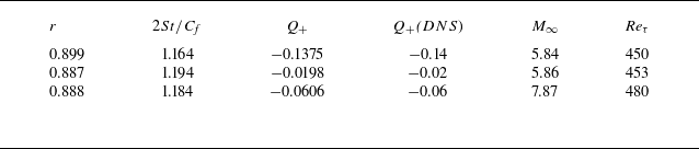
Formulas (6.5) and (6.16) allow us to calculate the wall heat flux from the known free-stream parameters, wall temperature and skin-friction coefficient. The results of calculations using the values of the constants from table 1 are presented in table 2 and yield values of
 $Q_+$
that are very close to those obtained by DNS (Zhang, Duan & Choudhari Reference Zhang, Duan and Choudhari2018). Moreover, as can be seen from table 2, good agreement is achieved despite the rather large free-stream Mach numbers.
Heat-flux values calculated with the help of formulas for the recovery and Reynolds-analogy factors (6.5) and (6.16) and the DNS data by Zhang et al. (Reference Zhang, Duan and Choudhari2018).

7. Velocity and temperature defect laws
According to (5.2) and (5.7), the velocity defect law in the outer region of the boundary layer is formulated in the same way as in an incompressible fluid (1.3), i.e. it is the von Kármán velocity defect law (Yaglom Reference Yaglom1979)
 \begin{align} \frac {u_\infty - \tilde u}{u_\infty \sqrt {\frac {1}{2} C_{\!f}}} = -\frac {f_0 (\eta )}{I_0} + O \big(\sqrt {C_{\!f}}\big). \end{align}
The temperature defect law on the basis of (5.12) and (5.15) has the form
 \begin{align} \frac {\tilde h - h_\infty }{\sigma u_\infty (u_\infty + q_w/\tau _w) \sqrt {\frac {1}{2} C_{\!f}}} = \varphi _0 (\eta ) + O \big(\sqrt {C_{\!f}}\big). \end{align}
Based on (6.14), this relation can be rewritten as
 \begin{align} \frac {\tilde h - h_\infty }{\big(h_w - h_\infty + \frac {1}{2} \sigma u_\infty ^2\big) \sqrt {\frac {1}{2} C_{\!f}}} = \varphi _0 (\eta ) + O \big(\sqrt {C_{\!f}}\big). \end{align}
This relationship also coincides with the following temperature defect law in an incompressible fluid (Vigdorovich Reference Vigdorovich2017):
 \begin{align} \frac {\overline h - h_\infty }{(h_w - h_\infty ) \sqrt {\frac {1}{2} C_{\!f}}} = \varphi _0 (\eta ) + O \big(\sqrt {C_{\!f}}\big), \end{align}
when the free-stream velocity squared can be neglected in comparison with the difference in enthalpy, i.e. in the special case
 $Ec = 0$
, corresponding to an incompressible fluid. The universal functions of the normalised distance from the wall on the right-hand sides of equalities (7.1) and (7.3) are the same as in an incompressible fluid.
Integrating equalities (7.1) and (7.3) across the layer and taking into account relations (3.10b ) and (3.13), we get
 \begin{align} \frac {\delta _u}{\sqrt {\frac {1}{2} C_{\!f}}} &= I_0 \delta \left [1 + O \big(\sqrt {C_{\!f}}\big) \right ]\!, \quad \frac {\sigma \delta _h}{\sqrt {\frac {1}{2} C_{\!f}}} = I_0 \delta \left [1 + O \big(\sqrt {C_{\!f}}\big) \right ]\!, \\\delta _u &= \int _0^\infty \left (1 - \frac {\tilde u}{u_\infty } \right ) \textrm {d} y, \quad \delta _h = \frac {\int _0^\infty (\tilde h - h_\infty ) \textrm{d}y}{h_w - h_\infty + \frac {1}{2} \sigma u_\infty ^2}, \nonumber \end{align}
where
 $\delta _u$
and
 $\delta _h$
are the velocity and enthalpy defect thicknesses. Hence, it is clear that, for the dynamical problem, it is convenient to use as a transverse scale the quantity
 $\delta _u \sqrt {2/C_{\!f}}$
, which for incompressible flow is known as the Clauser boundary-layer thickness (Clauser Reference Clauser1956) (see also Rotta Reference Rotta1950). For the thermal problem, such a role is played by the quantity
 $\delta _h \sqrt {2/C_{\!f}}$
, which in the special case
 $Ec = 0$
coincides with the characteristic transverse scale proposed for an incompressible fluid by Vigdorovich (Reference Vigdorovich2017). The relation between the dynamic and thermal scales is given by the equality
 \begin{align} \delta _u = \sigma \delta _h \left [ 1 + O \big(\sqrt {C_{\!f}}\big) \right ]\!, \end{align}
which gives an exact relationship between the integral parameters of the velocity and temperature profiles in turbulent boundary layers.
The range of applicability of the similarity laws (7.1) and (7.3) is the outer region of the boundary layer. We show that the velocity defect law that is satisfied everywhere outside the viscous sublayer can be written as
 \begin{align} \frac {\phi _\infty - \phi } {\tan \vartheta \sqrt {\frac {1}{2} C_{\!f}}} = - \frac {f_0 (\eta )}{I_0} \left [ 1 + O \big(\sqrt {C_{\!f}}\big) \right ]\!. \end{align}
The validity of this relationship in the outer region is proved by substitution of the expression for the velocity (5.2) into the left-hand side and expanding at
 $1/\eta = O(1)$
and
 $f_0 (\eta ) = O(1)$
in the small parameter
 $\zeta ^{-1}$
. This gives the expression
 \begin{align} - \frac {u_\infty \phi '(u_\infty ) \lambda _1 f_0 (\eta )}{\zeta \tan \vartheta \sqrt {\frac {1}{2} C_{\!f}}} + O(\zeta ^{-1}), \end{align}
which on the basis of (5.5) and (5.7) is equal to the right-hand side of (7.7). Let us now prove the validity of (7.7) for
 $\eta \to 0$
, i.e. in the logarithmic sublayer. In this region, the law of the wall (4.1b
) is satisfied. Let us recast the right-hand side of (4.1b
) in terms of
 $\eta$
using the formula
 $\ln y_+ = \ln \eta + \ln {\textit{Re}}_\tau$
and replace
 $\ln {\textit{Re}}_\tau$
by the expression (5.8). As a result, we obtain
 \begin{align} \frac {\phi _\infty - \phi } {\tan \vartheta \sqrt {\frac {1}{2} C_{\!f}}} + Q_1 (\phi _\infty ,\, \phi _w) - Q_1 (\phi ,\,\phi _w)= - \frac 1 \varkappa (\ln \eta + A_0 - \ln I_0). \end{align}
According to (3.10a
), the right-hand side of this equality is equal to the asymptotics of the right-hand side of (7.7) as
 $\eta \to 0$
. In the logarithmic region, where the difference
 $\phi _\infty - \phi$
is of order one, the first term on the left-hand side of (7.9) is a large quantity of order
 $C_{\!f}^{-1/2}$
and the second term is a quantity of order one. Therefore, (7.9) can be written as
 \begin{align} \frac {\phi _\infty - \phi } {\tan \vartheta \sqrt {\frac {1}{2} C_{\!f}}} \left [ 1 + O \big(\sqrt {C_{\!f}}\big) \right ] = - \frac 1 \varkappa (\ln \eta + A_0 - \ln I_0), \end{align}
which proves the validity of (7.7) in the logarithmic region.
The analogous to (7.7) temperature defect law reads
 \begin{align} \frac {\psi _\infty - \psi } {\tan \vartheta \sqrt {\frac {1}{2} C_{\!f}}} = \varphi _0 (\eta ) \left [ 1 + O \big(\sqrt {C_{\!f}}\big) \right ]\!. \end{align}
This relation can be proved in the same way as (7.7) using equalities (5.22), (4.1c ), (5.24) and (3.14). In the case of a heated and adiabatic plate, it is valid everywhere outside the viscous sublayer. But since, as stated above, in the boundary layer on a cooled plate, the law of the wall for temperature (4.1c ) describes the velocity profile only in the part of the logarithmic sublayer above the temperature maximum point, the temperature defect law (7.11) is also satisfied in the region above this point.
Let us now show that in the limit as
 $M_\infty \to 0$
and
 $h_w/h_\infty \to 1$
, relations (7.7) and (7.11) are the similarity laws for an incompressible fluid (7.1) and (7.4). Let us write the expansions of the functions
 $\phi (\tilde u)$
and
 $\psi (\tilde h)$
at the points
 $u_\infty$
and
 $h_\infty$
in power series with remainder terms:
 \begin{align} \phi &= \phi _\infty + \phi '(u_\infty ) (\tilde u - u_\infty ) + \frac 12 \phi ''(a) (\tilde u - u_\infty )^2 \nonumber \\ &= \phi _\infty + \phi '(u_\infty ) (\tilde u - u_\infty ) \left [ 1 + \frac {\phi ''(a)}{2 \phi '(u_\infty )} (\tilde u - u_\infty ) \right ]\!, \end{align}
 \begin{align} \psi &= \psi _\infty + \psi '(h_\infty ) (\tilde h - h_\infty ) + \frac 12 \psi ''(b) (\tilde h - h_\infty )^2 \nonumber \\ &= \psi _\infty + \psi '(u_\infty ) (\tilde h - h_\infty ) \left [ 1 + \frac {\psi ''(b)}{2 \psi '(u_\infty )} (\tilde h - h_\infty ) \right ]\!. \end{align}
Here
 $a$
and
 $b$
belong to the intervals
 $(\tilde u,\, u_\infty )$
and
 $(\tilde h,\, h_\infty )$
, respectively. Calculating the second derivative from (4.2) gives
 \begin{align} \phi ''(\tilde u) = - \frac {\sigma \tan \phi \cos ^2 \psi }{2 \tilde h \cos ^2 \phi }. \end{align}
In view of the value of the first derivative (5.5) as well as (4.5b
), (4.2) and (4.6) for the quantity in square brackets in (7.12a
), we can give the estimate
 $1 + O (\beta )$
,
 $\beta = h_w/h_\infty - 1$
and, thus, write
 \begin{align} \frac {\phi _\infty - \phi }{\tan \vartheta } = \left ( 1 - \frac {\tilde u}{u_\infty } \right ) [1 + O (\beta )], \quad M_\infty \to 0, \quad \frac {h_w}{h_\infty } \to 1. \end{align}
Therefore, in the limit under consideration, the left-hand sides of (7.7) and (7.1) coincide. Putting in (7.14)
 $\tilde u = 0$
and
 $\phi = \phi _w$
, we find that the limiting value of the quantity (5.11) is
 $\lambda _1 = \varkappa /F_0$
and is equal to the corresponding coefficient obtained by Vigdorovich (Reference Vigdorovich2017) for the incompressible boundary layer.
Based on (5.18), (5.23) and (4.5b ),
 \begin{align} \psi '(h_\infty ) = - \frac {\cot \psi _\infty }{2 h_\infty } = - \frac {\tan \vartheta }{\sigma u_\infty (u_\infty + q_w/\tau _w)}. \end{align}
Calculating the second derivative from (4.2b ), we have
 \begin{align} \psi ''(\tilde h) = - \frac {(\cot ^2 \psi - 1 ) \cot \psi }{4 \tilde h^2}. \end{align}
These expressions for the derivatives together with (4.5b
), (4.2) and (4.6) give for the quantity in square brackets in (7.12b
) the estimate
 $1 + O (Ec)$
. Therefore,
 \begin{align} \frac {\psi _\infty - \psi }{\tan \vartheta } = \frac {\tilde h - h_\infty }{h_w - h_\infty } [1 + O (Ec)], \quad M_\infty \to 0, \quad \frac {h_w}{h_\infty } \to 1. \end{align}
Since the Eckert number is small in incompressible flow, the left-hand sides of (7.11) and (7.4) coincide.
Thus, the velocity and temperature defect laws (7.7) and (7.11) are valid over the entire range of free-stream Mach numbers from zero to moderate supersonic values. According to (7.7) and (7.11), to calculate the universal velocity and enthalpy profiles, one needs to know the free-stream parameters as well as the enthalpy, heat flux and shear stress at the wall and only one empirical constant
 $\sigma$
.
The universal function on the right-hand side of (7.1) can be specified, e.g. using the empirical Coles formula known for the incompressible boundary layer (Coles Reference Coles1956),
 \begin{align} \frac {f_0 (\eta )} {I_0} = \frac 1 \varkappa \left [ \ln \eta - 0.55 (1 + \cos \pi \eta ) \right ]\!, \quad 0 \lt \eta \leqslant 1, \end{align}
in which the boundary-layer thickness
 $\delta$
is the distance from the wall at which the mean longitudinal velocity differs by
 $1 \,\%$
from the free-stream one. This relation yields
 $I_0 = 1.55/\varkappa$
and
 $A_0 = 0.23$
. If the analogue of the Clauser boundary-layer thickness (7.5a
) is used as the transverse scale, (7.18) becomes
 \begin{align} \frac {f_0 (\eta )}{I_0} = \frac 1 \varkappa \left [ \ln \left ( I_0 \sqrt {\frac {1}{2} C_{\!f}} \frac y {\delta _u} \right )- 0.55 - 0.55 \cos \left ( \pi I_0 \sqrt {\frac {1}{2} C_{\!f}} \frac y {\delta _u} \right ) \right ]\!. \end{align}
Vigdorovich (Reference Vigdorovich2017) showed that the function
 $\varphi _0 (\eta )$
is well approximated by the expression
 \begin{align} \varphi _0 (\eta ) = - \frac 1 \varkappa [\ln (\sigma \eta ) - 0.55 - 0.55 \cos (\pi \sigma \eta )], \quad 0 \lt \eta \leqslant \frac 1 \sigma , \end{align}
according to which the dimensionless temperature profile can be obtained from the velocity profile (7.18) by simply stretching the transverse coordinate by a factor of
 $1/\sigma$
. Unlike the relation given by Cebeci & Bradshaw (Reference Cebeci and Bradshaw1984), (7.20), in particular, accounts for the fact that the thicknesses of dynamic and thermal boundary layers are different. If according to (7.5b
),
 $\delta _h \sqrt {2/C_{\!f}}$
is used as the transverse scale, (7.20) reads
 \begin{align} \varphi _0 = - \frac 1 \varkappa \left [ \ln \left ( \sigma I_0 \sqrt {\frac {1}{2} C_{\!f}} \frac y {\delta _h} \right )- 0.55 - 0.55 \cos \left ( \pi \sigma I_0 \sqrt {\frac {1}{2} C_{\!f}} \frac y {\delta _h} \right ) \right ]\!. \end{align}
Equation (7.20) implies that
 $E_0 = A_0 + \ln \sigma$
.
7.1. About the averaging methods
The proposed theory is based on Favre’s averaging (Favre Reference Favre1969), since it preserves the form of the continuity equation (2.1b ). In experiments, Reynolds’ averaging is used to determine the velocity and temperature profiles. Therefore, before proceeding to the comparison with measurement data, we evaluate how the averaging method affects the magnitude of the parameters in the considered outer region of the boundary layer.
The equation of state for a perfect gas implies the equality
 \begin{align} \frac {p'}{\overline p} = \frac {\rho '}{\overline \rho } + \frac {h''}{\tilde h} + \frac {\rho ' h''}{\overline \rho \, \tilde h}, \end{align}
and from the definitions of Favre’s and Reynolds’ averaging we have
 \begin{align} \tilde u = \overline u \left ( 1 + \frac {\overline {\rho ' u'}}{\overline \rho \, \overline u} \right )\!, \quad \tilde h = \overline h \left ( 1 + \frac {\overline {\rho ' h'}}{\overline \rho \, \overline h} \right )\!. \end{align}
We will proceed from the estimates
 \begin{align} u' \thicksim u'' \thicksim \sqrt {\widetilde {u^{\prime \prime 2}}}, \quad h' \thicksim h'' \thicksim \sqrt {\widetilde {h^{\prime \prime 2}}}. \end{align}
Relations (2.3a ) and (2.3b ) allow us to estimate the magnitude of the root-mean-square fluctuations through the gradients of the mean quantities
 \begin{align} \sqrt {\widetilde {u^{\prime \prime 2}}} \thicksim y \frac {{\partial } \tilde u}{{\partial } y}, \quad \sqrt {\widetilde {h^{\prime \prime 2}}} \thicksim y \frac {{\partial } \tilde h} {{\partial } y}, \end{align}
which after calculation of these gradients from the velocity and enthalpy defect laws (7.1) and (7.3) yields
 \begin{align} \frac {u'}{u_\infty } \thicksim \sqrt {C_{\!f}}, \quad \frac {h'}{h_\infty } \thicksim M_\infty ^2 \sqrt {C_{\!f}}. \end{align}
Based on the pressure-fluctuation estimate
 $p' \thicksim \overline \rho u^{\prime 2}$
and relation (7.26a
), we obtain
 \begin{align} \frac {p'}{p_\infty } \thicksim M_\infty ^2 C_{\!f}. \end{align}
Hence, (7.22) and (7.26b ) give
 \begin{align} \frac {\rho '}{\overline \rho } \thicksim M_\infty ^2 \sqrt {C_{\!f}}. \end{align}
After substituting (7.26) and (7.28) into (7.23), we have in the outer region
 \begin{align} \tilde u = \overline u \left [1 + M_\infty ^2 O (C_{\!f}) \right ]\!, \quad \tilde h = \overline h \left [1 + M_\infty ^4 O (C_{\!f}) \right ]\!. \end{align}
Based on similar estimates of flow parameters in the logarithmic region, Vigdorovich (Reference Vigdorovich2023b ) obtained the relations that can be written as
 \begin{align} \tilde u = \overline u \left [1 + M_\infty ^2 O (C_{\!f}) \right ]\!, \quad \tilde h = \overline h \left [1 + M_\infty ^2 O (C_{\!f}) \right ]\!. \end{align}
Since the velocity and enthalpy defect laws (7.7) and (7.11) are formulated with an accuracy of
 $O(\sqrt {C_{\!f}})$
, relations (7.29) and (7.30) imply that at moderate Mach numbers, when
 $M_\infty = O(1)$
, these laws remain valid if Reynolds’ averaging is used instead of Favre’s averaging.
Conclusions about the small difference between the results of Favre’s and Reynolds’ averaging based on estimates partly employing empirical information are given by Cebeci & Bradshaw (Reference Cebeci and Bradshaw1984), and as a result of the analysis of the channel-flow DNS data are given by Huang et al. (Reference Huang, Coleman and Bradshaw1995).
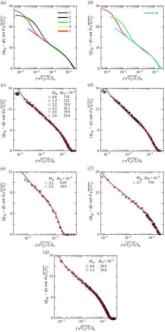
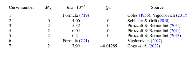
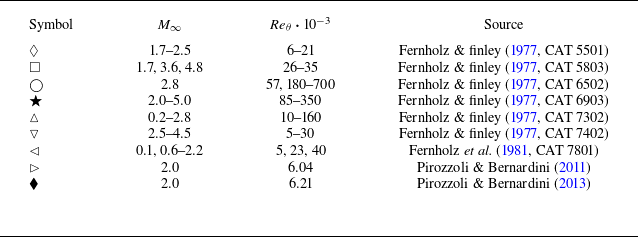
Calculated and experimental velocity and temperature profiles in subsonic and supersonic turbulent boundary layers on an adiabatic plate plotted in similarity variables (7.7) and (7.11). The description of the calculated curves is given in table 3. (c,d) Data from (Fernholz & Finley Reference Fernholz and Finley1977, CAT 7302), (e) data from (Fernholz & Finley Reference Fernholz and Finley1977, CAT 5501), (f) data from (Fernholz & Finley Reference Fernholz and Finley1977, CAT 6502), (g) data from (Fernholz, Finley & Mikulla Reference Fernholz, Finley and Mikulla1981, CAT 7801). The Reynolds number
 ${\textit{Re}}_\theta$
is calculated based on the free-stream parameters and momentum thickness.

7.2. Comparison with calculated and experimental data
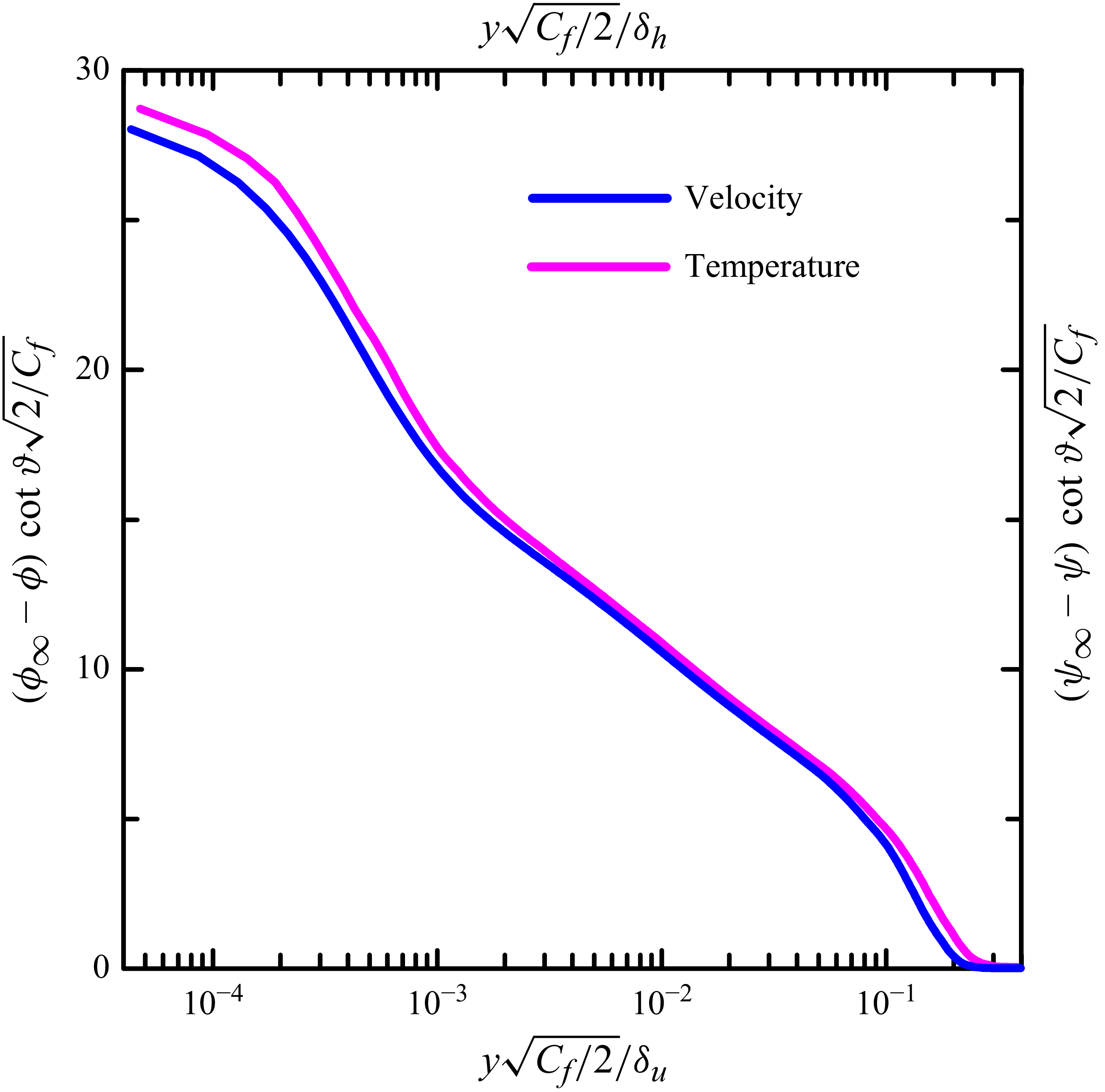
In figure 1 the velocity and temperature profiles in the turbulent boundary layer are plotted in the similarity variables (7.7) and (7.11), respectively. The quantities (7.5) are used as transverse scales. According to (7.7) and (7.11), the velocity and temperature profiles in the outer region and logarithmic sublayer are described by universal curves and, thus, do not depend on the free-stream Mach number (if, according to the assumptions made, it remains moderate and does not reach hypersonic values), Reynolds number and wall-heat-transfer conditions. The data in figure 1, obtained at zero wall heat flux, fully confirm the conclusions of the theory. In figure 1(a) the calculated velocity profiles in the incompressible (curve 2) (Schlatter & Örlü Reference Schlatter and Örlü2010) and compressible supersonic boundary layer at
 $M_\infty = 2$
(curves 3–5) (Pirozzoli & Bernardini Reference Pirozzoli and Bernardini2011, Reference Pirozzoli and Bernardini2013), outside the viscous sublayer, practically, describe a single curve, which can also be specified by the Coles formula for the incompressible boundary layer (7.19) (curve 1), while the Reynolds number affects only the logarithmic section extent. The temperature profiles obtained at
 $M_\infty = 2$
(figure 1
b) behave in the same way; in the outer region and logarithmic sublayer, they are very close to the empirical approximation of the temperature profile in the incompressible boundary layer (7.21). Complete universality in Mach and Reynolds numbers is demonstrated by the experimental data (Fernholz & Finley Reference Fernholz and Finley1977, CAT 7302) in figures 1(c,d), where all experimental points obtained at Mach numbers from
 $0.8$
to
 $2.8$
and different Reynolds numbers, outside the viscous sublayer lie on the calculated curves corresponding to
 $M_\infty = 2$
. The velocity profiles shown in figures 1(e–g), of which the profile in figure 1(f), in particular, corresponds to a very high Reynolds number
 ${\textit{Re}}_\theta = 7.34 \boldsymbol{\cdot }10^5$
and
 $M_\infty = 2.67$
, demonstrate the same behaviour.

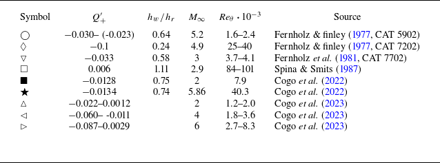
Calculated and experimental velocity and temperature profiles in supersonic turbulent boundary layers on a plate with heat transfer plotted in similarity variables (7.7) and (7.11). The calculated curves description is given in figure 1 and table 3. (c,d) Data from (Fernholz & Finley Reference Fernholz and Finley1977, CAT 7702) at
 $h_w/h_r = 0.58$
, (e, f) data from (Spina & Smits Reference Spina and Smits1987) at
 $h_w/h_r = 1.11$
and
 $M_\infty = 2.9$
.

The validity of the universal velocity and temperature defect laws (7.7) and (7.11) is confirmed by computational and experimental data obtained at non-zero wall heat transfer. Curve 7 in figure 2(a), which specifies the velocity profile on a cooled plate at
 $Q_+ = -0.01285$
,
 $h_w/h_r = 0.75$
and
 $M_\infty = 2$
(Cogo et al. Reference Cogo, Salvadore, Picano and Bernardini2022), outside the viscous sublayer is in perfect agreement with the velocity profile in the incompressible boundary layer (Schlatter & Örlü Reference Schlatter and Örlü2010). Furthermore, the corresponding temperature profile in figure 2(b) is quite close to the supersonic profile at zero heat flux (Pirozzoli & Bernardini Reference Pirozzoli and Bernardini2013) as well as the curve given by the empirical formula for an incompressible fluid (7.21). The experimental velocity and temperature profiles in figures 2(c,d), corresponding to
 $h_w/h_r = 0.58$
(Fernholz & Finley Reference Fernholz and Finley1977, CAT 7702), also follow the similarity rules (7.7) and (7.11). Across a cooled boundary layer, the temperature varies non-monotonically, so the temperature profiles plotted in similarity variables (7.11) in figures 2(b,d) have a local maximum in the logarithmic region. In figures 2(e, f) the velocity and temperature profiles measured in different sections of the boundary layer on a heated plate follow universal curves close to the profiles of the corresponding quantities in a zero-heat-flux boundary layer. Since the wall heat flux was not measured in this experiment, it is determined from the free-stream parameters, wall enthalpy and skin friction using (6.5) and (6.16) for the recovery and Reynolds-analogy factors. Figures 1 and 2 show that relations (7.7) and (7.11) provide universal velocity and temperature distributions up to
 $M_\infty = 3$
.
The temperature profiles in figures 1 and 2 follow empirical formula (7.21) and, thus, confirm the conclusion made by Vigdorovich (Reference Vigdorovich2017) that the temperature profile constructed in similarity variables can be obtained from the velocity profile by simply stretching the transverse coordinate by a factor of
 $1/\sigma$
. This empirical observation is consistent with the exact equality (7.6) that relates the integral parameters of the velocity and temperature profiles, and is confirmed by the DNS results – the calculated velocity and temperature profiles given in similarity variables in figure 3 are quite close.
Velocity and temperature profiles in similarity variables (7.7) and (7.11), respectively. The DNS data by Pirozzoli & Bernardini (Reference Pirozzoli and Bernardini2011) at
 $M_\infty = 2$
.

8. Similarity rules for quantities containing velocity and temperature fluctuations
Quantities containing velocity and enthalpy fluctuations can be expressed in terms of mean velocity and enthalpy gradients based on (2.2) and (2.3).
Differentiating both parts of equality (7.7) in view of the expression for the derivative (5.4) gives
 \begin{align} \frac {{\partial } \tilde u}{{\partial } y} \frac {y \cos \psi }{\cos \phi \tan \vartheta } \sqrt {\frac \sigma {\tilde h C_{\!f}}} = \frac {\eta f^{\prime}_0 (\eta )}{I_0} + O \big(\sqrt {C_{\!f}}\big). \end{align}
This equality, like the velocity defect law (7.7), from which it is obtained, is valid outside the viscous sublayer, i.e. in the logarithmic and outer regions, where, taking into account the estimates for the quantities
 $\varPi _1$
and
 $\varPi _2$
based on (2.4d
), we have
 \begin{align} U ({\textit{Re}},\, {\textit{Pe}},\, n,\, \eta ,\, \varPi _1,\, \varPi _2,\, \varGamma ) = U_0 (\infty ,\, \eta ) + O \big(\sqrt {C_{\!f}}\big). \end{align}
Relations (8.1) and (8.2) together with (2.3a ) allow us to obtain the representation for the root-mean-square velocity fluctuation
 \begin{align} \sqrt {\frac {2 h_\infty \widetilde {u^{\prime \prime 2}}} {\tilde h u_\infty ^2 C_{\!f}}} = \frac {\eta f^{\prime}_0 (\eta )}{I_0} \sqrt {U_0 (\infty ,\, \eta )} + O \big(\sqrt {C_{\!f}}\big). \end{align}
Here we also used equalities (4.5b ) and (4.6). The expressions for other Reynolds-tensor components are similar. Relation (8.3) is a similarity rule according to which, for moderate supersonic free-stream Mach numbers and any wall-heat-transfer conditions, the profile of the root-mean-square velocity fluctuation outside the viscous sublayer is described by a universal function of the dimensionless distance from the wall, which is known for an incompressible fluid.
The range of applicability of the similarity rule (8.3) can be extended to the entire boundary layer by writing it in the form
 \begin{align} \sqrt {\frac {2 \overline \rho \, \widetilde {u^{\prime \prime 2}}} {\rho _\infty u_\infty ^2 C_{\!f}}} = g (y_+, \, \eta ) + O \big(\sqrt {C_{\!f}}\big), \end{align}
where
 $g (y_+, \, \eta )$
is a universal function of two variables. Here we have also expressed the enthalpy ratio in terms of the density ratio, using the equation of state of the gas and the fact that, according to (3.17), the transverse pressure gradient in the boundary layer can be neglected. Relation (8.4), however, is not valid for all heat-transfer conditions but only for positive, zero and moderate negative wall heat flux, when, according to Vigdorovich (Reference Vigdorovich2023b
), the condition
 $q_w/(\tau _w \sqrt {2 h_w}) = O(1)$
is satisfied. In this case, the flow in the viscous sublayer is in the first approximation incompressible
 $\overline \rho /\rho _w = 1 + O (\sqrt {C_{\!f}})$
, while the dimensionless velocity profile is the same as in an incompressible fluid
 \begin{align} \frac {\tilde u}{u_\tau } = U_+ (y_+) + O (\varepsilon _*), \quad u_\tau = \sqrt {\frac {\tau _w}{\rho _w}}, \end{align}
and the variable characterising flow compressibility
 $\varPi _2 = O (\varepsilon _*)$
. Based on (8.5), (2.3a
) and (2.4d
), we obtain the representation
 \begin{align} \frac {\sqrt {\vphantom{{{u^{\prime \prime 2}}^{1}}}\widetilde {u^{\prime \prime 2}}}}{u_\tau } = y_+ \frac {\textrm {d} U_+}{\textrm {d} y_+} \sqrt {U_0 ({\textit{Re}},\, 0)} + O \big(\sqrt {C_{\!f}}\big), \quad {\textit{Re}} = y_+^2 \frac {\textrm {d} U_+}{\textrm {d} y_+}, \end{align}
which proves the validity of (8.4) in the viscous sublayer. In this region, the function on the right-hand side of (8.4) can be expressed in terms of the velocity profile in an incompressible fluid:
 \begin{align} g (y_+, \, 0) = y_+ \frac {\textrm {d} U_+}{\textrm {d} y_+} \sqrt {U_0 ({\textit{Re}},\, 0)}. \end{align}
Relation (8.4) as well as the similarity rules for other Reynolds-tensor components were obtained by Pirozzoli & Bernardini (Reference Pirozzoli and Bernardini2011) on the basis of the Morkovin (Reference Morkovin1962) hypothesis. For the same
 ${\textit{Re}}_\tau$
, relation (8.4) allows one to overlap the transverse Reynolds-tensor-component profiles in compressible and incompressible boundary layers, which was demonstrated with high accuracy by Pirozzoli & Bernardini (Reference Pirozzoli and Bernardini2011).
Differentiating both parts of equality (7.11), in view of the expression for the derivative (5.18), we get
 \begin{align} \frac {y \cot \psi }{\tilde h \tan \vartheta \sqrt {2 C_{\!f}}} \frac {{\partial } \tilde h}{{\partial } y} = \eta \varphi^{\prime}_{0} (\eta ) + O \big(\sqrt {C_{\!f}}\big). \end{align}
Like the temperature defect law (7.11), this relationship is valid everywhere outside the viscous sublayer for zero and positive wall heat flux, and when the heat flux is negative, it is valid above the point of maximum temperature. In this region, based on (2.3b
) and (2.4c
), replacing the function
 $G$
with the first term of the asymptotic expansion
 $G_0$
, we can write
 \begin{align} \frac {\cot \psi }{\tilde h \tan \vartheta } \sqrt {\frac {\widetilde {h^{\prime \prime 2}}}{2 C_{\!f}}} = -\eta \varphi^{\prime}_{0} (\eta ) \sqrt {G_0 (\infty ,\, \infty ,\, \eta )} + O \big(\sqrt {C_{\!f}}\big). \end{align}
On the right-hand side of this equality is a function of the dimensionless distance from the wall, known for the incompressible boundary layer. The similarity rule for the root-mean-square enthalpy fluctuation (8.9), as well as (8.3), is valid at moderate supersonic free-stream Mach numbers and any wall-heat-transfer conditions. In the particular case of an insulated plate, taking into account (4.2a ), it can be written as
 \begin{align} \frac {\sqrt {\vphantom{{{u^{\prime \prime 2}}^{1}}}\widetilde {h^{\prime \prime 2}}}}{\tan \vartheta \sqrt {2 \tilde h (h_r - \tilde h) C_{\!f}}} = -\eta \varphi^{\prime}_{0} (\eta ) \sqrt {G_0 (\infty ,\, \infty ,\, \eta )} + O \big(\sqrt {C_{\!f}}\big). \end{align}
The DNS data by Cogo et al. (Reference Cogo, Salvadore, Picano and Bernardini2022, Reference Cogo, Baù, Chinappi, Bernardini and Picano2023) plotted in figure 4 follow the similarity rule (8.9). The root-mean-square enthalpy fluctuation profiles obtained at
 $M_\infty = 2$
, different Reynolds numbers and different wall-heat-flux values describe one curve in the outer part of the boundary layer.
Direct numerical simulation data by Cogo et al. (Reference Cogo, Salvadore, Picano and Bernardini2022, Reference Cogo, Baù, Chinappi, Bernardini and Picano2023) for root-mean-square enthalpy fluctuations at
 $M_\infty = 2$
plotted in similarity variables (8.9). Curve 1:
 $Q_+ \approx 0$
; curve 2:
 $Q_+ = -0.0057$
and
 $Re_\tau = 444$
(Cogo et al. Reference Cogo, Baù, Chinappi, Bernardini and Picano2023); curve 3:
 $Q_+ = -0.01285$
and
 $Re_\tau = 1947$
(Cogo et al. Reference Cogo, Salvadore, Picano and Bernardini2022).

9. Skin-friction law
The matching of the velocity and temperature profiles yields two friction-law formulations (5.8) and (5.24). Since, based on (3.1), (5.1) and (7.5),
 \begin{align} I_0 {\textit{Re}}_\tau = I_0 {\textit{Re}}_\delta \sqrt {\frac {1}{2} C_{\!f}} = {\textit{Re}}_u \sqrt {\frac {h_\infty }{h_w}} \left [1 + O \big(\sqrt {C_{\!f}}\big) \right ] = \sigma {\textit{Re}}_h \sqrt {\frac {h_\infty }{h_w}} \left [1 + O \big(\sqrt {C_{\!f}}\big) \right ]\!, \end{align}
where
 ${\textit{Re}}_u = \rho _\infty u_\infty \delta _u/{\mu} _w$
and
 ${\textit{Re}}_h = \rho _\infty u_\infty \delta _h/{\mu} _w$
are the Reynolds numbers based on the free-stream parameters, wall viscosity and velocity and enthalpy defect thicknesses, which are given by the expressions (7.5), relations (5.8) and (5.24) can be written as
 \begin{align} \ln {\textit{Re}}_u &= \frac {\varkappa (\phi _\infty - \phi _w)} {\tan \vartheta \sqrt {\frac {1}{2} C_{\!f}}} + \varkappa [Q_1 (\phi _\infty ,\, \phi _w)- D_1 (\textit{Pr},\, n,\, Q_+)] + A_0 \nonumber\\ &\quad +\ \frac 12 \ln \frac {h_w}{h_\infty } + O \big(\sqrt {C_{\!f}}\big), \end{align}
 \begin{align} \ln (\sigma {\textit{Re}}_h) &= \frac {\varkappa (\psi _\infty - \phi _w)} {\tan \vartheta \sqrt {\frac {1}{2} C_{\!f}}} + \varkappa [R (\psi _\infty ,\, \phi _w) - D_1 (\textit{Pr},\, n,\, Q_+)] + E_0 \nonumber\\ &\quad +\, \frac 12 \ln \frac {h_w}{h_\infty } + O \big(\sqrt {C_{\!f}}\big). \end{align}
These equalities give an analytical formulation of the friction law, in which the Reynolds numbers are based on
 $\delta _u$
and
 $\delta _h$
(7.5), while the well-known empirical formulas for skin friction contain the momentum and energy thicknesses. This choice of characteristic transverse scales is dictated by the velocity and temperature defect laws (7.1) and (7.3), which allow us to express the boundary-layer thickness through integrals of the profiles of these quantities according to (7.5). Note that the quantity
 $\delta _u$
, which is calculated from the velocity defect, can be found in the extensive database (Fernholz & Finley Reference Fernholz and Finley1977; Fernholz et al. Reference Fernholz, Finley and Mikulla1981) along with other integral parameters of compressible boundary layers.
The definition of the function
 $\varLambda$
(3.2c
) and the expansion (3.5a
) imply that
 \begin{align} \textrm {d} {\textit{Re}}_x = \frac {\textrm {d} e^\xi }{\varLambda (\xi )} \sqrt {\frac {h_w}{h_\infty }} = \frac {\zeta \textrm {d} e^\xi }{\lambda _1} \sqrt {\frac {h_w}{h_\infty }} \big[1 + O(\zeta ^{-1}) \big], \quad {\textit{Re}}_x = \frac {\rho _\infty u_\infty x} {{\mu} _w}. \end{align}
Here,
 ${\textit{Re}}_x$
is the Reynolds number based on the distance from the leading edge of the plate. After integrating this expression and taking into account equality (5.7), we obtain
 \begin{align} {\textit{Re}}_x = \frac {\zeta {\textit{Re}}_\delta }{\lambda _1} \sqrt {\frac {h_w}{h_\infty }} \big[ 1 + O(\zeta ^{-1}) \big] = I_0 {\textit{Re}}_\delta \sqrt {\frac {2 h_w}{C_{\!f} h_\infty }} \big[ 1 + O \big(\sqrt {C_{\!f}}\big) \big]. \end{align}
Now, given relation (5.1) between
 ${\textit{Re}}_\tau$
and
 ${\textit{Re}}_\delta$
, equality (5.8) can be written as
 \begin{align} \ln {\textit{Re}}_x &= \frac {\varkappa (\phi _\infty - \phi _w)} {\tan \vartheta \sqrt {\frac {1}{2} C_{\!f}}} - \ln \frac {C_{\!f}} 2 + \varkappa [Q_1 (\phi _\infty ,\, \phi _w) - D_1 (\textit{Pr},\, n,\, Q_+)] + A_0 \nonumber\\ &\quad +\, \frac 12 \ln \frac {h_w}{h_\infty } + O \big(\sqrt {C_{\!f}}\big). \end{align}
9.1. Adiabatic plate
In the case of a thermally insulated plate, relations (9.2), taking into account the expressions for the functions
 $Q_1 (\phi _\infty ,\, 0)$
and
 $R (\psi _\infty ,\, 0)$
(4.1e
) and (4.1f
) and the equality
 $D_1 (\textit{Pr},\, n,\, 0) = D (\textit{Pr})$
, become
 \begin{align} \ln {\textit{Re}}_u &= \frac {\varkappa \phi _\infty \cot \vartheta }{\sqrt {\frac {1}{2} C_{\!f}}} + \varkappa A_1 \phi _\infty \tan \phi _\infty + (\varkappa A_3 - 1) \ln \cos \phi _\infty - \varkappa C + A_0 \nonumber\\ &\quad +\, O \big(\sqrt {C_{\!f}}\big), \nonumber\\ \ln (\sigma {\textit{Re}}_h)& = \frac {\varkappa \psi _\infty \cot \vartheta }{\sqrt {\frac {1}{2} C_{\!f}}} - \varkappa A_1 \psi _\infty \cot \psi _\infty + (\varkappa A_3 - 1) \ln \cos \psi _\infty - \varkappa (A_2 + C) \nonumber\\ &\quad +\, E_0 + O \big(\sqrt {C_{\!f}}\big). \end{align}
For
 $h_w = h_r$
, relations (4.2) on the basis of (4.5b
) yield
 \begin{align} \phi _\infty = \arcsin \frac {\sin \vartheta }{\sqrt {1 + (r/\sigma - 1) \sin ^2 \vartheta }}, \quad \psi _\infty = \arccos \frac {\cos \vartheta }{\sqrt {1 + (r/\sigma - 1) \sin ^2 \vartheta }}. \end{align}
Substituting here the expression for the recovery factor (6.5), after expanding in the small parameter
 $\sqrt {C_{\!f}}$
, we find that both relations (9.6) give the same expression, i.e.
 \begin{align} \ln {\textit{Re}}_u = \ln \sigma {\textit{Re}}_h &= \frac {\varkappa \vartheta \cot \vartheta }{\sqrt {\frac {1}{2} C_{\!f}}} + (\varkappa A_3 - 1) \ln \cos \vartheta \nonumber\\ &\quad +\, A_0 \cos ^2 \vartheta + (E_0 - \varkappa A_2) \sin ^2 \vartheta - \varkappa C + O \big(\sqrt {C_{\!f}}\big), \end{align}
while (9.5) is written as
 \begin{align} \ln {\textit{Re}}_x &= \frac {\varkappa \vartheta \cot \vartheta }{\sqrt {\frac {1}{2} C_{\!f}}} - \ln \frac {C_{\!f}} 2 + (\varkappa A_3 - 1) \ln \cos \vartheta \nonumber\\ &\quad + A_0 \cos ^2 \vartheta + (E_0 - \varkappa A_2) \sin ^2 \vartheta - \varkappa C + O \big(\sqrt {C_{\!f}}\big). \end{align}
For incompressible flow in the limit as
 $M_\infty \to 0$
(
 $\vartheta \to 0$
), relations (9.8) and (9.9) become
 \begin{align} \ln {\textit{Re}}_{\delta ^*} &= \frac \varkappa {\sqrt {\frac {1}{2} C_{\!f}}} - \varkappa C + A_0 + O \big(\sqrt {C_{\!f}}\big),\nonumber \\ \ln {\textit{Re}}_x &= \frac \varkappa {\sqrt {\frac {1}{2} C_{\!f}}} - \ln \frac {C_{\!f}} 2 - \varkappa C + A_0 + O \big(\sqrt {C_{\!f}}\big), \end{align}
where
 ${\textit{Re}}_{\delta ^*}$
is the Reynolds number based on the displacement thickness. These formulas for incompressible flow are given by Vigdorovich (Reference Vigdorovich2015).
Thus, when
 $M_\infty$
ranges from zero (incompressible flow) to moderate supersonic values, the skin-friction coefficient on an adiabatic wall is a known function of the Reynolds number
 ${\textit{Re}}_u$
,
 ${\textit{Re}}_h$
or
 ${\textit{Re}}_x$
, free-stream Mach number and heat capacity ratio (see (4.5b
) for the quantity
 $\vartheta$
), as well as seven universal constants, five of which, i.e.
 $\varkappa$
,
 $C$
,
 $\sigma$
,
 $A_0$
and
 $E_0$
, are known for incompressible flow, and the two
 $A_2$
and
 $A_3$
are included in the laws of the wall for velocity and temperature for a compressible gas (Vigdorovich Reference Vigdorovich2024). Here, it should be emphasised again that according to (9.8) and (9.9), the skin-friction coefficient on an adiabatic plate does not depend on the molecular Prandtl number.
Expressing the skin-friction coefficient from equality (9.8), we obtain
 \begin{align} \sqrt {\frac {1}{2} C_{\!f}} = \frac {\varkappa \vartheta \cot \vartheta }{\ln {\textit{Re}}_u + (1 - \varkappa A_3) \ln \cos \vartheta - A_0 \cos ^2 \vartheta + (\varkappa A_2 - E_0) \sin ^2 \vartheta + \varkappa C}. \end{align}


In figure 5, this formula is compared with a large body of experimental data collected by Fernholz & Finley (Reference Fernholz and Finley1977), Fernholz et al. (Reference Fernholz, Finley and Mikulla1981) and the DNS data of Pirozzoli & Bernardini (Reference Pirozzoli and Bernardini2011, Reference Pirozzoli and Bernardini2013). As can be seen in table 4, which shows the range of Mach and Reynolds numbers in which the experiments were performed, it describes well the measurement results up to
 $M_\infty = 5$
.
Description of experimental and calculated points in figure 5.

9.2. Heat transfer at the wall
In the case of non-zero wall heat flux, the friction law in the form (9.2) contains one empirical function
 $D_1 (\textit{Pr},\, n,\, Q_+)$
, which depends on the dimensionless heat flux
 $Q_+$
, molecular Prandtl number and viscosity law (Vigdorovich Reference Vigdorovich2024). According to (4.2) and (4.4), the quantities
 $\phi _w$
,
 $\phi _\infty$
,
 $\psi _\infty$
and
 $Q_+$
included in (9.2) are calculated based on the wall-heat-flux value
 $q_w$
. If this quantity is unknown or is not determined accurately enough, which is quite typical of available experimental data (Fernholz & Finley Reference Fernholz and Finley1977; Fernholz et al. Reference Fernholz, Finley and Mikulla1981; Spina & Smits Reference Spina and Smits1987), it can be determined from the known free-stream parameters, skin friction and wall enthalpy using the formulas for the recovery and Reynolds-analogy factors (6.5) and (6.16).
In view of (4.5b ) and (6.7), (4.3) can be written as
 \begin{align} \tan \phi _w = \alpha \tan \vartheta \frac {2 - r Ec}{2 Ec} \sqrt {\frac {h_\infty }{h_w}}. \end{align}
Substituting here the expressions for the recovery and Reynolds-analogy factors (6.5), (6.16) and expanding in the small parameter
 $\sqrt {C_{\!f}}$
, we have
 \begin{align} \tan \phi _w &= \tan \phi ^{\prime}_w - N \sqrt {\frac {1}{2} C_{\!f}} + O(C_{\!f}), \\N &= \frac 12 \sec \psi ^{\prime}_\infty \sec \phi ^{\prime}_w \left [ P(\psi ^{\prime}_\infty ,\,\phi ^{\prime}_w) + \frac 1 \varkappa (A_0 - E_0) \sin 2 \psi ^{\prime}_\infty \right ]\!. \nonumber \end{align}
Here, we have taken into account the expression (6.15a ) and the representations (4.2). From (9.13), we obtain
 \begin{align} \phi _w = \phi ^{\prime}_w - \cos ^2 \phi ^{\prime}_w N \sqrt {\frac {1}{2} C_{\!f}} + O(C_{\!f}). \end{align}
Relations (4.2b ) and (9.14) imply that
 \begin{align} \psi _\infty = \psi ^{\prime}_\infty - \frac 12 \sin 2 \phi ^{\prime}_w \cot \psi ^{\prime}_\infty N \sqrt {\frac {1}{2} C_{\!f}} + O(C_{\!f}). \end{align}
Equalities (9.14) and (9.15) yield
 \begin{align} \frac {\psi _\infty - \phi _w} {\sqrt {\frac {1}{2} C_{\!f}}} = \frac {\psi ^{\prime}_\infty - \phi ^{\prime}_w}{\sqrt {\frac {1}{2} C_{\!f}}} + \frac {\cos \phi ^{\prime}_w \sin \big(\psi ^{\prime}_\infty - \phi ^{\prime}_w\big) N}{\sin \psi ^{\prime}_\infty } + O\big(\sqrt {C_{\!f}}\big). \end{align}
Substituting this relation into (9.2b ), we obtain the skin-friction law, which is valid at moderate free-stream Mach numbers over the entire range of wall heat flux,
 \begin{align} \varkappa D_1 \big(\textit{Pr},\, n,\, Q_{+}^{\prime }\big) = &\, \frac {\varkappa \big(\psi ^{\prime}_\infty - \phi ^{\prime}_w\big)}{\tan \vartheta \sqrt {\frac {1}{2} C_{\!f}}} - \ln {\textit{Re}}_u + \frac {\varkappa A_1 \big(\psi ^{\prime}_\infty - \phi ^{\prime}_w\big)}{\tan \vartheta } \left ( \sqrt {\frac {h_w}{h_\infty }} - 1 \right ) \nonumber\\ & +\, \left \{ A_0 - E_0 + \varkappa A_2 + \varkappa [D (\textit{Pr}) - C - A_2] \sqrt {\frac {h_w}{h_\infty }} \right \} \frac {\sin \big(\psi ^{\prime}_\infty - \phi ^{\prime}_w\big)}{\tan \vartheta }\nonumber \\ & +\, \frac 12 (1 - \varkappa A_3) \ln \frac {h_w}{h_\infty } + E_0 + O(\sqrt {C_{\!f}}), \end{align}
where in view of (9.1),
 ${\textit{Re}}_u$
can be replaced by
 $\sigma {\textit{Re}}_h$
. According to this equality, its right-hand side, which can be calculated from the Reynolds number, skin-friction coefficient, wall enthalpy and free-stream parameters, for fixed
 $\textit{Pr}$
and
 $n$
, is a function of only the quantity
 \begin{align} Q_{+}^{\prime } = \frac 2 \sigma \tan \phi ^{\prime}_w \tan \vartheta \sqrt {\frac {1}{2} C_{\!f}}, \end{align}
which based on (4.3) and (4.4) represents the quantity
 $Q_+$
with the accuracy
 $O (\sqrt {C_{\!f}})$
and may also be calculated in terms of the skin-friction coefficient, wall enthalpy and free-stream parameters. In other words, the skin-friction distribution can be described by a single universal curve that is specified by the function
 $D_1 (\textit{Pr},\, n,\, Q_{+}^{\prime })$
.
Since in all available experiments and calculations
 $Q_{+}^{\prime }$
is a sufficiently small quantity (see table 5), after expanding in the series
 \begin{align} D_1 (\textit{Pr},\, n,\, Q_{+}^{\prime }) = D (\textit{Pr}) - d (\textit{Pr},\, n) Q_{+}^{\prime } + O(Q_{+}^{\prime 2}), \quad d (\textit{Pr},\, n) = - \frac {{\partial } D_1 (\textit{Pr},\, n,\, 0)}{{\partial } Q_+} \end{align}
the left-hand side of (9.17) taking into account (9.18) can be written as
 \begin{align} \varkappa D (\textit{Pr}) - \frac {2 \varkappa } \sigma d (\textit{Pr},\, n) \tan \phi ^{\prime}_w \tan \vartheta \sqrt {\frac {1}{2} C_{\!f}}. \end{align}
This transforms (9.17) into an equation for the skin-friction coefficient, which contains one unknown parameter
 $d (\textit{Pr},\, n)$
, the value of the derivative of the function
 $D_1 (\textit{Pr},\, n,\, Q_+)$
at
 $Q_+ = 0$
. As a result of processing the velocity profiles in the logarithmic region of boundary layers based on the law of the wall (4.1b
), Vigdorovich (Reference Vigdorovich2024) obtained the estimate for this quantity
 $d (\textit{Pr},\, n) \approx 22$
, which will be used further.
Description of experimental and calculated points in figure 6.


The solution of (9.17) with the right-hand side (9.20) is
 \begin{align} &\qquad\sqrt {\frac {1}{2} C_{\!f}} = \frac {2 a}{\sqrt {c^2 + 4 a b} + c}, \end{align}
 \begin{align} &\qquad\qquad a = \varkappa \big(\psi ^{\prime}_\infty - \phi ^{\prime}_w\big), \quad b = - \frac {2 \varkappa } \sigma d (\textit{Pr},\, n) \tan \phi ^{\prime}_w \tan ^2 \vartheta , \end{align}
 \begin{align} c &= \tan \vartheta \left [ \ln {\textit{Re}}_u - \frac 12 (1 - \varkappa A_3) \ln \frac {h_w}{h_\infty } + \varkappa D (\textit{Pr}) - E_0 \right ] \nonumber \\ &\quad - \varkappa A_1 \big(\psi ^{\prime}_\infty - \phi ^{\prime}_w\big) \left ( \sqrt {\frac {h_w}{h_\infty }} - 1 \right )\nonumber \\ &\quad - \left \{ A_0 - E_0 + \varkappa A_2 + \varkappa [D (\textit{Pr}) - C - A_2] \sqrt {\frac {h_w}{h_\infty }} \right \} \sin \big(\psi ^{\prime}_\infty - \phi ^{\prime}_w\big). \end{align}
In figure 6 this formula is compared with available experimental and DNS data for the boundary layer on a cooled and heated plate. For the derivative
 $d (\textit{Pr},\, n)$
, the above value is adopted, also given in table 1. It can be seen that (9.21) generally describes the experimental and calculated data well. The maximum inaccuracy is observed at the largest heat-flux values (see table 5), which is natural given the assumption under which this formula is obtained from exact relation (9.17) where
 $D_1 (\textit{Pr},\, n,\, Q_+)$
is approximated by a linear function. Although even at the heat-flux value
 $Q_{+}^{\prime } = -0.1$
, for which
 $h_w/h_r = 0.24$
, the discrepancy does not exceed
 $10\, \%$
. The agreement between the theory and available experimental and calculated data is observed up to
 $M_\infty = 6$
.
10. Conclusion and discussion
We develop a rational asymptotic theory of the compressible turbulent boundary layer on a flat plate, whose first main element are closure relations connecting the Reynolds-tensor components and turbulent enthalpy flux with the mean velocity and enthalpy gradients. Together with the boundary layer and energy equations, they give a well-posed boundary-value problem for the mean velocity and enthalpy fields (Vigdorovich Reference Vigdorovich2023a ). Derived from first principles, these closure relations are not based on any partial hypotheses about the nature of turbulent exchange or turbulence models and, therefore, allow us to describe the flow under consideration at a new higher level of rigour.
The second important element of the theory is its asymptotic character. When describing the flow in the near-wall region, we introduce a small parameter of the problem
 $\varepsilon _*$
, which is proportional to the Mach number formed with the friction velocity and the speed of sound at the wall, and construct the solution in two characteristic regions of the boundary layer – viscous and logarithmic – by the method of matched asymptotic expansions in this small parameter (Vigdorovich Reference Vigdorovich2023b
, Reference Vigdorovich2024).
For an asymptotic description of the flow under consideration in the outer region and the boundary layer as a whole, a special change of variables in the boundary-layer and energy equations is proposed, which makes it possible to construct the solution in the form of asymptotic expansions at large values of the logarithm of the Reynolds number based on the boundary-layer thickness. Together with the results known for an incompressible fluid (see, e.g. Vigdorovich Reference Vigdorovich1993, Reference Vigdorovich2017), this, in particular, shows that an adequate small parameter for near-wall turbulent flows is the reciprocal of the logarithm of Reynolds number.
The velocity and temperature defect laws, valid in the range of free-stream Mach numbers from zero to moderate supersonic values, are obtained in two forms, which have different ranges of applicability. The linear form (7.1) and (7.3) is valid only in the outer region, while the nonlinear form (7.7) and (7.11) is true everywhere outside the viscous sublayer, i.e. in the outer and logarithmic regions of the boundary layer. The linear form (7.1) and (7.3) is convenient for calculating the characteristic transverse scales of the dynamic and thermal boundary layer, since it allows these quantities to be represented in terms of the velocity and enthalpy defect thicknesses.
At moderate free-stream Mach numbers, the compressibility of the flow in the outer region can be neglected, and in similarity variables the velocity and temperature profiles are the same as in an incompressible fluid. Comparison with calculated and experimental data shows that the universal velocity and temperature defect laws (7.7) and (7.11) are valid up to
 $M_\infty = 3$
.
Asymptotically exact (and therefore most reliable) expressions for the recovery and Reynolds-analogy factors obtained in this work, in addition to their general theoretical significance, also have important practical applications. Thus, there is a substantial corpus of experimental data for turbulent boundary layers in supersonic flow (Fernholz & Finley Reference Fernholz and Finley1977; Fernholz et al. Reference Fernholz, Finley and Mikulla1981). The measurements were performed in boundary layers on adiabatic surfaces and in the presence of wall heat transfer. However, in the latter case, there are practically no reliable data for the wall heat flux. In most experimental works, the heat-flux values are not given at all, and only the wall temperature is measured. However, the skin-friction-coefficient value is almost always known. Knowing the recovery and Reynolds-analogy factors allows us, by calculating the Stanton number from the skin-friction coefficient, then to determine heat flux from the difference between the recovery and wall temperatures. The results of such calculations, given in table 2, agree very well with the DNS data.
The friction law, which is expressed by relations (9.2), is formulated as a functional relationship between the Reynolds number, heat flux and shear stress at the wall, as well as the free-stream and wall parameters of the gas. These asymptotically exact relations, in contrast to the known semi-empirical formulas, use integral parameters calculated from the velocity or enthalpy defects as the transverse scale of the boundary layer. At moderate Mach numbers, they allows us to describe the skin-friction distribution by a single universal curve, which is specified by the empirical function
 $D_1 (\textit{Pr},\, n,\, Q_+)$
. At zero heat flux, relations (9.2) together with the expression for the recovery factor yield a simple formula for the skin-friction coefficient, which describes well available experimental and computational data up to
 $M_\infty = 5$
. For non-zero heat transfer, the formulas for the recovery and Reynolds-analogy factors allow us to reduce the number of parameters included in the friction law by excluding wall heat flux. Given the fact that in all available experiments and calculations the dimensionless heat flux
 $Q_+$
is a sufficiently small quantity and the function
 $D_1 (\textit{Pr},\, n,\, Q_+)$
can be replaced by its two-term expansion in zero, this gives an explicit formula for the skin-friction coefficient, which also describes the available experimental data up to
 $M_\infty = 6$
quite well. The only free parameter used in this approximation, the derivative
 $D_1 (\textit{Pr},\, n,\, Q_+)$
at zero, is taken from the work of Vigdorovich (Reference Vigdorovich2024), where it is determined by processing the velocity profiles in the logarithmic region of the boundary layer. The formulas for skin friction do not contain any fitting coefficients that are present in all known empirical formulas, while the empirical constants that are included in them are either long known (
 $\varkappa$
,
 $\sigma$
, etc.), or, like
 $A_1$
,
 $A_2$
and
 $A_3$
, were determined in earlier works (Vigdorovich Reference Vigdorovich2023b
, Reference Vigdorovich2024) from comparison with velocity and temperature profiles.
The obtained by Vigdorovich (Reference Vigdorovich2023a ) representations for the quantities containing velocity and temperature fluctuations (2.2) and (2.3), together with the velocity and temperature defect laws (7.7) and (7.11), give the similarity rules for the Reynolds-tensor components obtained earlier by Pirozzoli & Bernardini (Reference Pirozzoli and Bernardini2011) on the basis of the Morkovin (Reference Morkovin1962) hypothesis, as well as a new similarity rule for the root-mean-square enthalpy fluctuation.
Acknowledgements
The author would like to thank S. Pirozzoli and M. Bernardini, who kindly provided their DNS data.
Funding
The paper is published with the financial support of the Ministry of Education and Science of the Russian Federation as part of the program of the Moscow Center for Fundamental and Applied Mathematics under the Agreement no. 075-15-2025-345.
Declaration of interests
The author reports no conflict of interest.