1 Introduction
High-strength polymer fibres are produced by a solution spinning technique wherein the polymeric fluid filament is stretched mechanically while being exposed to air. For high tensile strength, it is desired that the globular molecular chains be stretched and aligned in the axial direction. The stretching is achieved by mechanically drawing the filament from the spinneret through the air gap before winding it onto the rotating spool. The strength of the extensional flow in the air gap is characterised by the parameter termed the draw ratio
 $DR$
, defined as the ratio of fibre velocity at the take-up point (controlled by the speed of the rotating spool) to the velocity at the spinneret (extrudate velocity at the die-exit point). Very thin fibres are produced by subjecting the fluid to high draw ratio. However, for draw ratio higher than a certain critical value
 $DR_{c}$
, the extensional spinning flow admits travelling wave instability known as draw resonance, which manifests in the form of sustained oscillations in the fibre cross-sectional area at any point in the air gap (Christensen Reference Christensen1962). Draw resonance can be understood kinematically as the progression of a throughput wave along the spinline which travels faster than the fluid residence time in the air gap (Hyun Reference Hyun1978). The critical draw ratio
 $DR_{c}$
for the onset of the instability, is strongly influenced by fluid rheology under extensional flow conditions. In realistic fibre spinning, the filament of polymeric solution exits the spinneret at a very high temperature (above the polymer crystallisation temperature), and it loses both heat energy and solvent as it travels towards the take-up roller. This heat and mass transfer from fibre to the ambient air greatly influences the fluid rheology which in turn affects the stability behaviour of the spinning flow. In this study, the role of simultaneous heat and mass transfer in draw resonance is investigated using both linear and weakly nonlinear stability analyses.
For Newtonian fluid under creeping flow and isothermal conditions, the onset of draw resonance occurs at the critical draw ratio of 20.218 (Matovich & Pearson Reference Matovich and Pearson1969; Pearson & Matovich Reference Pearson and Matovich1969; Fisher & Denn Reference Fisher and Denn1975a
, Reference Fisher and Denn1976). This value of
 $DR_{c}$
is independent of the length of spinning flow and the extrudate velocity. It is also independent of the viscosity of the Newtonian fluid, provided that viscosity remains constant throughout the evaluation domain. For viscoelastic fluids described using the upper convected Maxwell (UCM) model, studies have found that the critical draw ratio depends on the fluid elasticity characterised by the flow Deborah number defined as
 $De=\unicode[STIX]{x1D706}v_{0}/L$
(Hyun Reference Hyun1999; Jung & Hyun Reference Jung and Hyun1999; Lee et al.
Reference Lee, Jung, Hyun and Scriven2005a
). Here,
 $\unicode[STIX]{x1D706}$
is the characteristic relaxation time of the fluid,
 $v_{0}$
is the extrudate velocity through the die exit and
 $L$
is the length of the air gap. The enhancement in extensional viscosity for the polymeric fluid leads to
 $DR_{c}$
values greater than
 $20.218$
indicating the stabilising role of fluid elasticity. Under non-isothermal spinning, Jung & Hyun (Reference Jung and Hyun1999) found that the cooling decreases the sensitivity of spinline tension to perturbations indicating stabilisation by heat transfer. However, a simple Maxwell model more suitable for unentangled polymer fails to appropriately describe the rheological behaviour of high- and ultra-high-molecular-weight entangled polymer. In particular, the Maxwell model is unable to capture the nonlinear extensional rheology of high-molecular-weight polymers due to the divergence of extensional viscosity, even for a moderate strength of extensional flow, making it unsuitable for high-speed fibre spinning.
For a solution of high-molecular-weight entangled polymers, both strain rate thinning and strain rate hardening effects are realised depending upon the strength of extensional flow characterised by Deborah number. Therefore, a viscoelastic model is desired which captures the nonlinear rheological behaviour shown by polymer solutions. This analysis employs the eXtended Pom-Pom (XPP) model, a variant of the classical tube model, for the dynamics of entangled polymers which is known to predict both rate hardening and softening and spans well across elastic flows of interest for high-strength fibre spinning (Inkson et al. Reference Inkson, McLeish, Harlen and Groves1999; Verbeeten, Peters & Baaijens Reference Verbeeten, Peters and Baaijens2001). The XPP model has been used extensively to describe the dynamics of entangled polymers (Auhl et al. Reference Auhl, Hoyle, Hassell, Lord and Harlen2011; van der Walt et al. Reference van der Walt, Hulsen, Bogaerds, Meijer and Bulters2012; Gupta & Chokshi Reference Gupta and Chokshi2015, Reference Gupta and Chokshi2016, Reference Gupta and Chokshi2017). It should be noted that the XPP model can produce non-physical multiple solutions in simple steady shear and uniaxial extensional flows, when the anisotropy parameter is non-zero (Clemeur, Rutgers & Debbaut Reference Clemeur, Rutgers and Debbaut2003; Inkson & Phillips Reference Inkson and Phillips2007). For this analysis, the anisotropy parameter is kept at zero since the second normal stress difference is ignored, and this suppresses the occurrence of multiple steady states (Baltussen Reference Baltussen2010; Baltussen, Hulsen & Peters Reference Baltussen, Hulsen and Peters2010).
While the previous analysis (Gupta & Chokshi Reference Gupta and Chokshi2015) assumes a uniform temperature and concentration of polymer along the spinline, the practical fibre spinning process is usually accompanied by an axial temperature drop and solvent evaporation in the air gap. The simultaneous transfer of thermal energy and solvent to the surrounding air results in considerable enhancement of fluid viscosity, whose effect on stability behaviour is the focus of the present study. The analysis by Gupta & Chokshi (Reference Gupta and Chokshi2015) established that that spinline stability is directly correlated to the fluid rheology. The neutral stability curve exhibits the stabilising effect of strain rate hardening and destabilising effect of strain rate softening in different flow regimes. The experiments by Yang & Chen (Reference Yang and Chen1997) on an ultra-high-molecular-weight polyethylene (UHMWPE)–decalin system show that the change in viscosity can be as much sensitive to the variation in concentration as it is to the variation in temperature, and hence, both these factors are expected to play a significant role in the spinline stability. This sensitivity however, can be desirably altered by introducing additives into the polymer matrix that influence the activation energy. A series of experiments show that filaments/films produced by solution spinning of a UHMWPE–decalin system are more drawable than melt spinning of UHMWPE under similar drawing conditions and have superior mechanical properties (Smith & Lemstra Reference Smith and Lemstra1979, Reference Smith and Lemstra1980a ,Reference Smith and Lemstra b ,Reference Smith and Lemstra c ; Smith, Lemstra & Booij Reference Smith, Lemstra and Booij1981). For pure melt spinning too, experiments by Ishihara & Kase (Reference Ishihara and Kase1976) demonstrated suppressed perturbation amplitudes with increasing spinline length, due to the increasing dominance of cooling. For viscoelastic fluids described by the UCM model, Fisher & Denn (Reference Fisher and Denn1977) constructed stability map in an ambient temperature–Stanton number plane indicating the stabilising role of heat transfer. The experimental and theoretical studies by Demay & Agassant (Reference Demay and Agassant1985) also confirm the enhancement in flow stability with increasing heat transfer.
The simultaneous heat and mass transfer during fibre spinning has been analysed for dry spinning (Ohzawa, Nagano & Matsuo Reference Ohzawa, Nagano and Matsuo1969; Ohzawa & Nagano Reference Ohzawa and Nagano1970). In dry (solution) spinning, the solidification of fibre is entirely achieved in a long air gap by evaporation of the solvent and convective cooling by surrounding air. In gel (melt) spinning, heat convection in the short air gap may only solidify the filament partially, and complete solidification is achieved by quenching in water/chemical bath. In the former case of dry spinning, the phase transition of polymer from solution to semi-crystalline state occurs in the air gap itself, such that the polymer crystallisation becomes important. Lee et al. (Reference Lee, Shin, Jung and Hyun2005b
) examined the role of flow induced crystallisation in the dynamics of the low-speed fibre spinning process. For the latter case of gel spinning, the short air gap is insufficient for crystallisation. If the temperature of the spinline is held above the crystallisation temperature (or glass transition
 $T_{g}$
for amorphous polymers), the cooling of the spinline has a stabilising influence on draw resonance (Matsumoto & Bogue Reference Matsumoto and Bogue1978). This stabilisation is attributed to the enhancement in the extensional viscosity of the polymer due to a reduction in temperature. Thus, the rheology, in terms of sensitivity of viscosity to temperature, plays an important role in the onset of draw resonance.
The stability analysis of fibre spinning with external heating has gained significant interest in the recent past (Blyler Jr & Gieniewski Reference Blyler and Gieniewski1980). For spinning of Newtonian fluids under external heating, the theoretical studies by Wylie, Huang & Miura (Reference Wylie, Huang and Miura2007) and Suman & Kumar (Reference Suman and Kumar2009) indicate multiple steady states, specifically three values of spinning force for a given draw ratio. The multiplicity is caused due to the abrupt change in fluid viscosity upon heating, modelled as a near-step function of viscosity with temperature. This multiplicity introduces a qualitatively new thermo-viscous instability for a small window of heating flux and spinning force which strongly depends on the magnitude and abruptness of the step-like variation in viscosity with temperature. For viscoelastic fluids described by the simple upper convected Maxwell model with a step-like variation in viscosity with temperature, Zhou & Kumar (Reference Zhou and Kumar2010) found that heating stabilises the spinline for lower elasticity indicated by the critical draw ratio of above 20.2, the corresponding isothermal value. For fluids with high elasticity, the authors find that the multiplicity in steady state is eliminated and the non-isothermal effect exhibits a destabilising influence on draw resonance.
The high-strength polymer fibres are produced by the gel spinning technique with a short air gap to induce high extensional strain rates. The spinline loses thermal energy by convective heat transfer to the ambient air and also by removal of latent heat due to solvent evaporation. In the present study, the role of thermal effects on the onset of draw resonance is investigated with the help of linear stability analysis. It is important to quantify the role of individual effects, viz. convective effect and solvent evaporation, in the stability behaviour. For isothermal spinning, Gupta & Chokshi (Reference Gupta and Chokshi2015) show that the spinning flow is Hopf bifurcated at the critical draw ratio, and the nature of bifurcation is supercritical for low to moderate elasticity and crosses over to the subcritical unstable state for high elasticity. The present work also performs the weakly nonlinear stability analysis to predict the bifurcation and amplitude of disturbances in the vicinity of the critical point and examine the role of thermal effects on the finite amplitude stability of fibre spinning.
The rest of the paper is organised as follows: § 2 provides the mathematical formulation of the problem being studied. In this section, a model to describe the temperature and concentration dependence of fluid rheology is presented. This section also outlines the theoretical framework of both linear and weakly nonlinear stability analyses. The results are discussed in § 3, by assuming exemplary spinning data for a polyethylene–decalin (polymer–solvent) system. The effect of simultaneous heat and mass transfer on the steady state as well as the linear stability of the system is then examined. Lastly, the finite amplitude stability analysis of the extensional spinning flow is presented. The equilibrium amplitude of a resonating spinline post-onset of draw resonance is also estimated to analyse the role of thermal effects on stability characteristics. The important findings are summarised and concluded in § 4.
2 Problem formulation
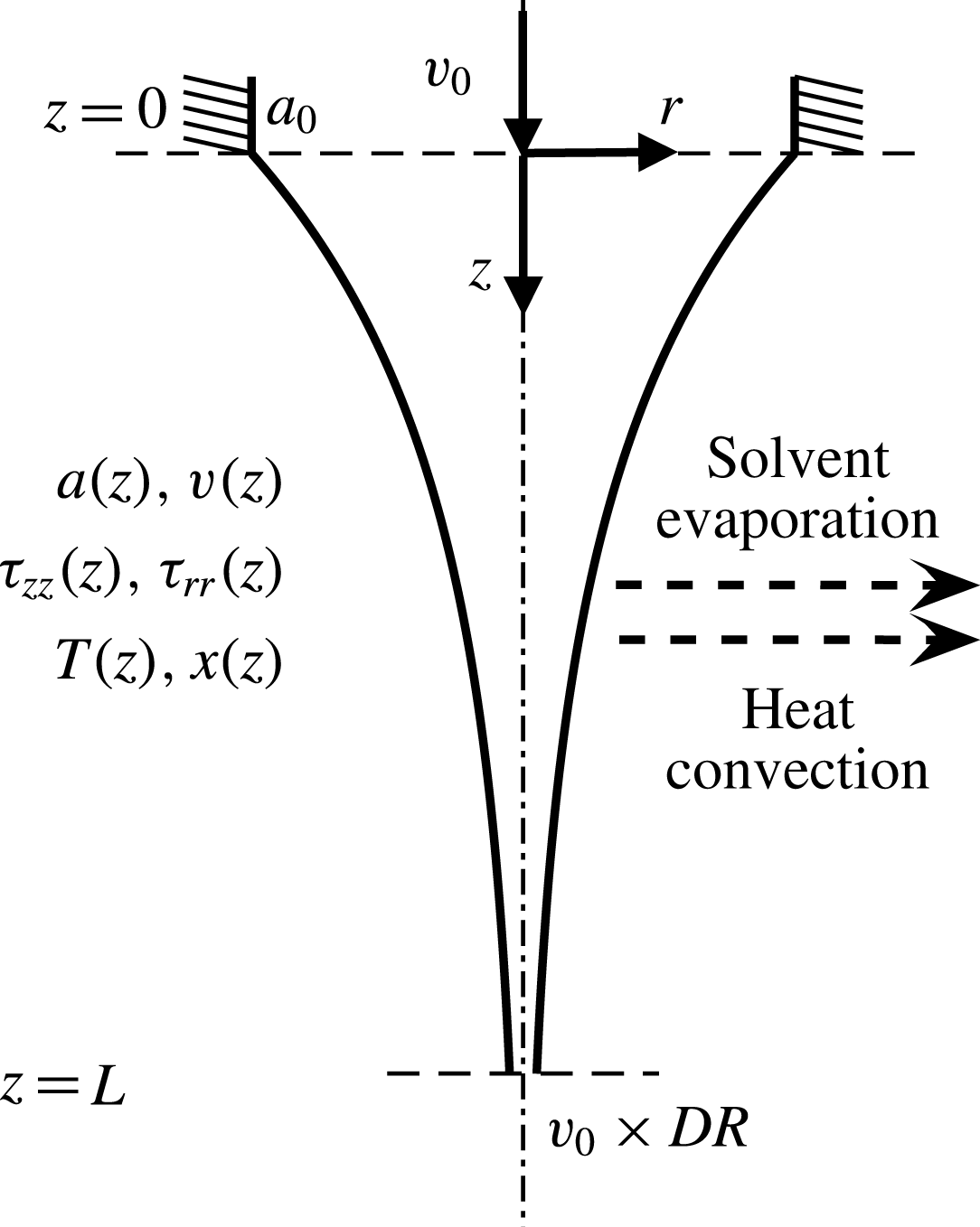
In polymer fibre spinning process, a concentrated solution of high-molecular-weight entangled polymer flows through the spinneret (die-exit point) from which a filament is drawn. The filament is subject to significant thinning to obtain thin fibres with polymeric chains aligned along the fibre axis. The chain alignment is responsible for high mechanical strength post crystallisation/solidification. The drawing of fibre takes place in the air gap, as shown in figure 1, at the end of which the fibre is quenched in water bath before being wound on a take-up roller. In the spinline, the polymeric fluid is subjected to a strong extensional flow with exposure to ambient air. While drawing, the filament loses thermal energy to the surrounding air by convective cooling. In addition, the solvent also evaporates in air resulting in further cooling by the loss of latent heat. The spinline usually releases heat and mass to a natural (stationary) environment, although a cooling air flow may also be used. Thus, the spinning flow exhibits a significant temperature and concentration variation along the spinline as the fibre thins. It is, however, assumed that the fibre temperature does not drop below its crystallisation temperature and the polymeric material essentially remains in the liquid state.
Schematic of an air-gap flow in fibre spinning process showing the one-dimensional coordinate system. The flow begins at the extrusion point (
 $z=0$
) and terminates at the take-up end (
 $z=L$
). Area
 $a$
, velocity
 $v$
, axial
 $\unicode[STIX]{x1D70F}_{zz}$
and radial
 $\unicode[STIX]{x1D70F}_{rr}$
stresses, temperature
 $T$
and polymer mass fraction
 $x$
are only dependent on axial position
 $z$
. The ratio of take-up to extrusion speed is termed the draw ratio
 $DR$
. The spinline loses both heat and solvent to the ambient air by convection and evaporation mechanisms.

2.1 Mathematical modelling
In the present study, the predominant elongational air-gap flow from the point of maximum extrudate swell near the die exit (
 $z=0$
) to the take-up point (
 $z=L$
) is considered. The spinning flow is modelled as a one-dimensional slender-body filament assuming that the spinline variables are functions of only the axial direction, and the radial distribution of the fibre variables, like velocity and temperature, are ignored. For the spinning flow considered, the length of the air gap is typically 25–100 mm and the radius of the capillary is 0.5 mm. Therefore, the aspect ratio of the fibre is around 50–200, justifying the slender-body approximation. Considering the polymeric flow means viscoelastic stresses are dominant, and other forces like inertia, gravity and surface tension are negligible and are hence ignored. Further, material properties such as density, specific heat and thermal conductivity are assumed to be constant along the fibre axis. For this analysis, non-isothermal conditions are considered. Thus the spinline is gradually exchanging heat by three mechanisms – convection, evaporation and viscous dissipation (radiation negligible) – as it progresses from the spinneret to take-up. The loss of thermal energy is not significant enough to cause crystallisation however, i.e. the temperature of spinline remains well above the crystallisation temperature. Also, there is negligible heat conduction within the spinline in the axial direction. Lastly, the extrudate swell exhibited by the spinline is neglected for this study, and hence the domain starts from the point of maximum extrudate swell. The influence of extrudate swell on stability for this fibre spinning model is studied in Gupta & Chokshi (Reference Gupta and Chokshi2016).
In the present study, simultaneous heat and mass transfer effects on the spinline stability are studied, since the spinline loses not only heat but also the solvent mass to the environment. Thus, the spinline variables considered are: fibre cross-sectional area
 $a(z)$
, fibre velocity
 $v(z)$
, stresses
 $\unicode[STIX]{x1D749}(z)$
, temperature
 $T(z)$
and mass fraction of polymer
 $x(z)$
. The dimensional governing equations are
 $$\begin{eqnarray}\displaystyle & \displaystyle \unicode[STIX]{x1D70C}\frac{\unicode[STIX]{x2202}a}{\unicode[STIX]{x2202}t}+\unicode[STIX]{x1D70C}\frac{\unicode[STIX]{x2202}(av)}{\unicode[STIX]{x2202}z}=-2\sqrt{a\unicode[STIX]{x03C0}}N, & \displaystyle\end{eqnarray}$$
 $$\begin{eqnarray}\displaystyle & \displaystyle \unicode[STIX]{x1D70C}\frac{\unicode[STIX]{x2202}}{\unicode[STIX]{x2202}t}[(1-x)a]+\unicode[STIX]{x1D70C}\frac{\unicode[STIX]{x2202}}{\unicode[STIX]{x2202}z}[av(1-x)]=-2\sqrt{a\unicode[STIX]{x03C0}}N, & \displaystyle\end{eqnarray}$$
 $$\begin{eqnarray}\displaystyle & \displaystyle \frac{\unicode[STIX]{x2202}}{\unicode[STIX]{x2202}z}(a\unicode[STIX]{x1D6F4}_{zz})=0, & \displaystyle\end{eqnarray}$$
 $$\begin{eqnarray}\displaystyle & \displaystyle \unicode[STIX]{x1D70C}C_{p}\left[\frac{\unicode[STIX]{x2202}(aT)}{\unicode[STIX]{x2202}t}+\frac{\unicode[STIX]{x2202}(avT)}{\unicode[STIX]{x2202}z}\right]=-2\sqrt{a\unicode[STIX]{x03C0}}[h(T-T_{a})+N{\mathcal{L}}]+a\unicode[STIX]{x1D6F4}_{zz}\frac{\unicode[STIX]{x2202}v}{\unicode[STIX]{x2202}z}, & \displaystyle\end{eqnarray}$$
 $$\begin{eqnarray}\displaystyle & \displaystyle \frac{\unicode[STIX]{x2202}\unicode[STIX]{x1D749}}{\unicode[STIX]{x2202}t}+\boldsymbol{v}\boldsymbol{\cdot }\unicode[STIX]{x1D735}\unicode[STIX]{x1D749}-\unicode[STIX]{x1D749}\boldsymbol{\cdot }\unicode[STIX]{x1D735}\boldsymbol{v}-(\unicode[STIX]{x1D735}\boldsymbol{v})^{\text{T}}\boldsymbol{\cdot }\unicode[STIX]{x1D749}=G[(\unicode[STIX]{x1D735}\boldsymbol{v})+\left(\unicode[STIX]{x1D735}\boldsymbol{v}\right)^{\text{T}}]-\frac{1}{\unicode[STIX]{x1D706}}[F\unicode[STIX]{x1D749}+G(F-1)\unicode[STIX]{x1D644}],\quad & \displaystyle\end{eqnarray}$$
 $$\begin{eqnarray}\displaystyle & \displaystyle \text{where }F=2r\left(1-\frac{1}{\unicode[STIX]{x1D6EC}}\right)\exp \left[\frac{2}{q}(\unicode[STIX]{x1D6EC}-1)\right]+\frac{1}{\unicode[STIX]{x1D6EC}^{2}},\text{and }\unicode[STIX]{x1D6EC}^{2}=1+\frac{\text{tr}(\unicode[STIX]{x1D749})}{3G}. & \displaystyle\end{eqnarray}$$
Equation (2.1) is the overall mass conservation equation, and (2.2) is the conservation equation for the solvent species. Equations (2.3) and (2.4) are the momentum and thermal energy conservation equations.
 $\unicode[STIX]{x1D6F4}_{zz}$
is the total normal stress in the
 $z$
-direction given by
 $\unicode[STIX]{x1D6F4}_{zz}=\unicode[STIX]{x1D70F}_{zz}-\unicode[STIX]{x1D70F}_{rr}$
. The polymeric stress tensor
 $\unicode[STIX]{x1D749}$
is described by the XPP model, the nonlinear rheological model given in (2.5). The superscript
 $\text{T}$
denotes the transpose. The various terms in the above governing equations (2.1)–(2.5) will be explained next.
In the mass conservation equations,
 $N$
is the mass flux of the solvent evaporating from the spinline given by the film theory as
 $$\begin{eqnarray}N=m\unicode[STIX]{x1D70C}(1-x),\end{eqnarray}$$
where
 $m$
is the mass transfer coefficient. The evaporation mass flux removes the latent heat from the spinline and hence it also appears in the energy conservation equation (2.4). In this equation,
 ${\mathcal{L}}$
is the latent heat of solvent evaporation. The change in thermal energy can also occur due to convective heat transfer from the fibre to the surrounding air (either stationary or flowing). The temperature change due to convective heat transfer is given by the term containing
 $h$
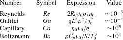
, the heat transfer coefficient. The last term in (2.4) is the viscous dissipation term. The heat transfer by radiation is considered insignificant. In the momentum balance equation (2.3), the forces like inertia, gravity and surface tension are ignored in comparison to the dominant viscous forces. This assumption can be justified by calculating the typical dimensionless numbers for the spinline in table 1, from the assumed variable values specified later in table 2. For the dominant viscous forces in the polymeric spinline, the spinning force, given by
 ${\mathcal{F}}=a\unicode[STIX]{x1D6F4}_{zz}$
, remains constant along the spinline.
Typical dimensionless numbers for the spinline.

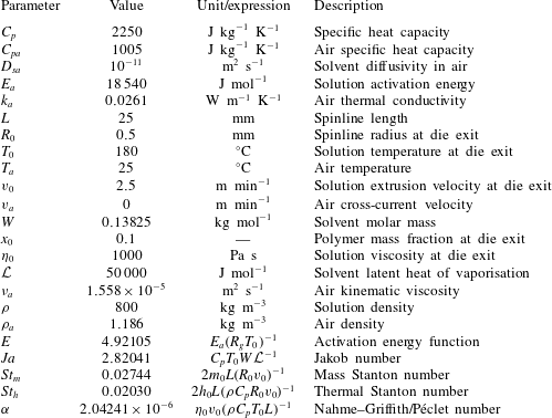
Polymer and ambient air properties, and the calculated dimensionless numbers for the reference non-isothermal UHMWPE–decalin fibre spinning case.

The above governing equations (2.1)–(2.5) include an appropriate constitutive equation which describes the rheology of an entangled polymer. The present study employs a variant of the tube model (Doi & Edwards Reference Doi and Edwards1978), the XPP model (Verbeeten et al.
Reference Verbeeten, Peters and Baaijens2001). The XPP model, given in (2.5), describes the nonlinear rheology of an entangled polymer and it captures the realistic dynamics of polymeric flow under both shear and extension. The XPP model has been extensively employed to describe the dynamics of entangled polymers (Auhl et al.
Reference Auhl, Hoyle, Hassell, Lord and Harlen2011; van der Walt et al.
Reference van der Walt, Hulsen, Bogaerds, Meijer and Bulters2012; Gupta & Chokshi Reference Gupta and Chokshi2015, Reference Gupta and Chokshi2017). The XPP model considers a polymeric chain to be composed of two parts, a backbone chain, and the free dangling arms present at each end of the backbone. To reptate, a chain must retract the branches to the retraction point (local branch point). The function
 $F$
in the XPP constitutive equation (2.5) contains the effect of chain architecture. The number of arms
 $q$
at each end of the XPP molecule physically signify the resistance faced by the backbone to reptate (strain hardening), while the ratio of relaxation times
 $r$
signify the separation of time scales for the two modes of chain movement, i.e. backbone orientation and stretch.
 $\unicode[STIX]{x1D6EC}$
is a measure of the extent of chain stretch.
Since the rheology of the material varies along the spinline due to variation in temperature and concentration, a proper estimation of the material properties is necessary. In real fibre spinning processes, the viscosity is known to be dependent on the concentration and temperature. This dependence is shown in the experiments performed by Yang & Chen (Reference Yang and Chen1997) for a solution of ultra-high-molecular-weight polyethylene (UHMWPE) dissolved in decalin solvent. For the UHMWPE–decalin solution in the regime
 $T\gg T_{g}$
of interest, the authors propose the expression
 $$\begin{eqnarray}\unicode[STIX]{x1D702}=\unicode[STIX]{x1D702}_{0}\left(\frac{x}{x_{0}}\right)^{3}\exp \left[\frac{E_{a}}{R_{g}}\left(\frac{1}{T}-\frac{1}{T_{0}}\right)\right]=\unicode[STIX]{x1D702}_{0}\unicode[STIX]{x1D709}(T,x).\end{eqnarray}$$
The subscript ‘
 $0$
’ refers to the value of the variables at the spinneret end at
 $z=0$
. This expression was proposed for a UHMWPE concentration of less than
 $10\,\%$
by weight, for which case the solution viscosity is found to depend on concentration by a simple power law. The temperature dependence of viscosity is given by the Arrhenius–Frenkel–Eyring relation in the range
 $125{-}165\,^{\circ }\text{C}$
. These are typical conditions for the presented analysis, and thus the chosen viscosity model is suitable. The model is advantageous in a sense that, a simple empirical relation can adequately model the change in extensional viscosity imparted by changes in concentration and temperature, and also by introduction of additives (changing activation energy) that influence the polymer chain–solvent interactions. The relation is, however, of limited suitability for a dilute solution of UHMWPE in decalin
 $(x<0.1)$
. Now, since the temperature dependence of elastic modulus of a polymeric fluid is given by
 $G\propto k_{B}T$
(Rubinstein & Colby Reference Rubinstein and Colby2007; Dealy & Plazek Reference Dealy and Plazek2009), one can write
 $$\begin{eqnarray}G=G_{0}T/T_{0}.\end{eqnarray}$$
Thus, the longest relaxation time of the XPP molecule
 $\unicode[STIX]{x1D706}$
is defined as
 $$\begin{eqnarray}\unicode[STIX]{x1D706}=\frac{\unicode[STIX]{x1D702}}{G}=\frac{\unicode[STIX]{x1D702}_{0}}{G_{0}}\frac{\unicode[STIX]{x1D709}}{T/T_{0}}=\unicode[STIX]{x1D706}_{0}\frac{\unicode[STIX]{x1D709}}{T/T_{0}}.\end{eqnarray}$$
The above three relations (2.8)–(2.10) describe the dependence of the material properties on the change in temperature and composition, thus influencing the rheology of the material. This influence modifies the XPP constitutive equation (2.5) to yield terms containing the temperature variable
 $T$
and viscosity function
 $\unicode[STIX]{x1D709}$
, discussed later in the non-dimensionalised and resolved XPP equations (2.21)–(2.22). By uniaxial extension calculations, the temperature and composition dependent XPP constitutive equation exhibits an enhanced extensional hardening characteristic.
The developed model considers that the spinline dissipates energy in an environment that may be natural, or forced by a cooling air flow. The transfer coefficients are expected to change as the spinline proceeds from the spinneret to the take-up. Thus, the heat and the mass transfer coefficients can be given by
 $$\begin{eqnarray}\displaystyle & \displaystyle h=h_{0}\unicode[STIX]{x1D713}(a,v,v_{a}), & \displaystyle\end{eqnarray}$$
 $$\begin{eqnarray}\displaystyle & \displaystyle m=m_{0}\unicode[STIX]{x1D713}(a,v,v_{a}), & \displaystyle\end{eqnarray}$$
with
 $h_{0}$
and
 $m_{0}$
being the transfer coefficients at the spinneret end
 $(z=0)$
. The heat and mass transfer coefficients vary along the spinline as given by the function
 $\unicode[STIX]{x1D713}(a,v,v_{a})$
, where
 $v_{a}$
denotes the speed of the surrounding air. For a fine cylindrical filament cooled by an air current,
 $\unicode[STIX]{x1D713}(a,v,v_{a})$
is derived by Kase & Matsuo (Reference Kase and Matsuo1967) as
 $$\begin{eqnarray}\unicode[STIX]{x1D713}(a,v,v_{a})=\left(\frac{v}{a}\right)^{1/3}\left[1+\left(\frac{8v_{a}}{v}\right)^{2}\right]^{1/6}=\left(\frac{v^{2}+64v_{a}^{2}}{a^{2}}\right)^{1/6}.\end{eqnarray}$$
The transfer coefficients are not only influenced by the fibre velocity and area, but also by the orientation of the cooling air speed with respect to the spinline as given by the ratio
 $v_{a}/v$
, which is the tangent of the angle which the cooling air makes with the spinline. Since
 $v=v(z)$
, this angle can be interpreted as an incident angle of a single stream of cooling air on a stationary particle at the spinline surface. For
 $v_{a}=0$
meaning no cross-air at all, the cooling air draft is co-current to the flow of spinline by virtue of motion of the spinline itself in a cooled stagnant environment. As
 $v_{a}$
increases, the cooling air becomes increasingly cross-current, until at
 $v_{a}=\infty$
the flow is exactly cross-current. As further explained by Kase & Matsuo (Reference Kase and Matsuo1967), cooling of the top segment of the spinline is dominated by
 $v_{a}$
, while the cooling of lower segment is dominated by the spinline velocity
 $v$
. Along the spinline where
 $v_{a}/v=0.125$
, transition of this dominance takes place.
Now, the initial transfer coefficients
 $h_{0}$
and
 $m_{0}$
need to be estimated. For the fibre spinning process,
 $m_{0}$
is derived from the heat transfer–mass transfer analogy, given by (Ohzawa et al.
Reference Ohzawa, Nagano and Matsuo1969)
 $$\begin{eqnarray}m_{0}=h_{0}\left(\frac{\unicode[STIX]{x1D70C}_{a}D_{sa}}{k_{a}}\right)\left(\frac{Sc}{Pr}\right)^{1/2}=h_{0}\left(\frac{D_{sa}}{\unicode[STIX]{x1D70C}_{a}C_{pa}k_{a}}\right)^{1/2},\end{eqnarray}$$
where the subscript ‘
 $a$
’ refers to the ambient air properties.
 $Sc=\unicode[STIX]{x1D708}_{a}/D_{sa}$
and
 $Pr=C_{pa}\unicode[STIX]{x1D708}_{a}\unicode[STIX]{x1D70C}_{a}/k_{a}$
are the Schmidt and the Prandtl numbers respectively.
 $D_{sa}$
is the solvent diffusivity in air. Now, for air flowing past a fine cylindrical filament of any polymer type with circular cross-section,
 $h_{0}$
is derived to be (Kase & Matsuo Reference Kase and Matsuo1967)
 $$\begin{eqnarray}h_{0}=0.388\left(\frac{k_{a}}{\unicode[STIX]{x1D708}_{a}^{1/3}}\right)\left(\frac{v_{0}}{a_{0}}\right)^{1/3}.\end{eqnarray}$$
Next, the fibre variables are made dimensionless as follows:
 $$\begin{eqnarray}a^{\ast }=\frac{a}{a_{0}},\quad v^{\ast }=\frac{v}{v_{0}},\quad \unicode[STIX]{x1D70F}_{zz}^{\ast }=\frac{\unicode[STIX]{x1D70F}_{zz}}{G_{0}},\quad \unicode[STIX]{x1D70F}_{rr}^{\ast }=\frac{\unicode[STIX]{x1D70F}_{rr}}{G_{0}},\quad T^{\ast }=\frac{T}{T_{0}},\quad z^{\ast }=\frac{z}{L},\quad t^{\ast }=t\frac{v_{0}}{L}.\end{eqnarray}$$
The variables with superscript ‘
 $\ast$
’ denote dimensionless variables. In what follows, the superscript ‘
 $\ast$
’ is dropped for brevity. The non-dimensionalised governing equations become
 $$\begin{eqnarray}\displaystyle & \displaystyle \frac{\unicode[STIX]{x2202}a}{\unicode[STIX]{x2202}t}+\frac{\unicode[STIX]{x2202}(av)}{\unicode[STIX]{x2202}z}=-St_{m}\sqrt{a}(1-x)\unicode[STIX]{x1D713}, & \displaystyle\end{eqnarray}$$
 $$\begin{eqnarray}\displaystyle & \displaystyle \frac{\unicode[STIX]{x2202}x}{\unicode[STIX]{x2202}t}+v\frac{\unicode[STIX]{x2202}x}{\unicode[STIX]{x2202}z}=\frac{St_{m}}{\sqrt{a}}x(1-x)\unicode[STIX]{x1D713}, & \displaystyle\end{eqnarray}$$
 $$\begin{eqnarray}\displaystyle & \displaystyle \frac{\unicode[STIX]{x2202}(a\unicode[STIX]{x1D6F4}_{zz})}{\unicode[STIX]{x2202}z}=0, & \displaystyle\end{eqnarray}$$
 $$\begin{eqnarray}\displaystyle & \displaystyle \frac{\unicode[STIX]{x2202}T}{\unicode[STIX]{x2202}t}+v\frac{\unicode[STIX]{x2202}T}{\unicode[STIX]{x2202}z}=-\frac{\unicode[STIX]{x1D713}}{\sqrt{a}}\left[St_{h}(T-T_{a})+\frac{St_{m}(1-x)}{Ja}\right]+\unicode[STIX]{x1D6FC}\frac{\unicode[STIX]{x1D6F4}_{zz}}{De}\frac{\unicode[STIX]{x2202}v}{\unicode[STIX]{x2202}z}, & \displaystyle\end{eqnarray}$$
 $$\begin{eqnarray}\displaystyle & \displaystyle \frac{\unicode[STIX]{x2202}\unicode[STIX]{x1D70F}_{zz}}{\unicode[STIX]{x2202}t}+v\frac{\unicode[STIX]{x2202}\unicode[STIX]{x1D70F}_{zz}}{\unicode[STIX]{x2202}z}-2(\unicode[STIX]{x1D70F}_{zz}+T)\frac{\unicode[STIX]{x2202}v}{\unicode[STIX]{x2202}z}=-\frac{T}{De\unicode[STIX]{x1D709}}[F\unicode[STIX]{x1D70F}_{zz}+T(F-1)], & \displaystyle\end{eqnarray}$$
 $$\begin{eqnarray}\displaystyle & \displaystyle \frac{\unicode[STIX]{x2202}\unicode[STIX]{x1D70F}_{rr}}{\unicode[STIX]{x2202}t}+v\frac{\unicode[STIX]{x2202}\unicode[STIX]{x1D70F}_{rr}}{\unicode[STIX]{x2202}z}+(\unicode[STIX]{x1D70F}_{rr}+T)\frac{\unicode[STIX]{x2202}v}{\unicode[STIX]{x2202}z}=-\frac{T}{De\unicode[STIX]{x1D709}}[F\unicode[STIX]{x1D70F}_{rr}+T(F-1)], & \displaystyle\end{eqnarray}$$
 $$\begin{eqnarray}\displaystyle & \displaystyle \text{where }F=2r\left(1-\frac{1}{\unicode[STIX]{x1D6EC}}\right)\exp \left[\frac{2}{q}\left(\unicode[STIX]{x1D6EC}-1\right)\right]+\frac{1}{\unicode[STIX]{x1D6EC}^{2}},\text{and }\unicode[STIX]{x1D6EC}^{2}=1+\frac{\unicode[STIX]{x1D70F}_{zz}+2\unicode[STIX]{x1D70F}_{rr}}{3T}.\qquad & \displaystyle\end{eqnarray}$$
Note that the ambient temperature
 $T_{a}$
is also made dimensionless by
 $T_{0}$
in the energy conservation equation (2.20). The various dimensionless groups appearing in the governing equations (2.17)–(2.22) are explained next.
(i)
 $\unicode[STIX]{x1D713}=(v^{2}+64v_{a}^{2})^{1/6}/a^{1/3}$
accounts for the effect of the velocity and the orientation of the cooling air on the energy loss to the environment by the spinline, as explained in the discussion for (2.13).
(ii)
$St_{m}=(2m_{0}L)/(R_{0}v_{0})$
is the mass Stanton number, accounting for the energy lost by the spinline to the environment, by the solvent evaporation mode.(iii)
$St_{h}=(2h_{0}L)/(\unicode[STIX]{x1D70C}C_{p}R_{0}v_{0})$
is the thermal Stanton number, accounting for the spinline’s energy loss to the environment by the convection mode. By substituting the expression for
$h_{0}$
from (2.15) here, it can be seen that this form of
$St_{h}$
agrees with the one used extensively in the literature, as
$St_{h}=cL/(\unicode[STIX]{x1D70C}C_{p}a_{0}^{5/6}v_{0}^{2/3})$
, where
$c$
is a constant (Fisher & Denn Reference Fisher and Denn1977; Jung, Song & Hyun Reference Jung, Song and Hyun1999).(iv)
$Ja=C_{p}T_{0}W/{\mathcal{L}}$
is the ratio of the sensible heat contained in the polymer to the latent energy
${\mathcal{L}}$
expelled during liquid–vapour phase change, where
$W$
is the solvent molar mass.(v)
$\unicode[STIX]{x1D6FC}=(\unicode[STIX]{x1D702}_{0}v_{0})/(\unicode[STIX]{x1D70C}C_{p}T_{0}L)$
is the ratio of Nahme–Griffith to Péclet number, characterising the heat generated due to viscous dissipation in the bulk of the system.(vi)
$De=\unicode[STIX]{x1D706}_{0}v_{0}/L$
is the Deborah number, a measure of fluid elasticity, such that for
$De\ll 1$
, the polymer chains are neither stretched nor oriented and hence the fluid behaves like a Newtonian fluid.(vii)
$\unicode[STIX]{x1D709}=(x/x_{0})^{3}\exp [E(1/T-1)]$
accounts for the effect of the temperature and composition change on the polymer rheology (viscosity and relaxation time) due to energy and mass lost to the environment by the spinline, as explained in the discussion for (2.8).(viii)
$E=E_{a}/(R_{g}T_{0})$
is the dimensionless activation energy appearing in the Arrhenius term in the expression for
$\unicode[STIX]{x1D709}$
.(ix)
$F$
and
$\unicode[STIX]{x1D6EC}^{2}$
are the viscoelastic terms appearing in the XPP constitutive equation (2.21) and (2.22).














While the present analysis holds qualitatively for a general polymer–solvent system, as a case study, the spinning fluid is considered to be ultra-high-molecular-weight polyethylene dissolved in decalin solvent (Yang & Chen Reference Yang and Chen1997; Clément & Leng Reference Clément and Leng2004). The material parameters for the UHMWPE–decalin system are given in table 2, where the values of the various dimensionless numbers appearing in the analysis are also listed.
For stability analysis, the steady-state solution of the above nonlinear equations is first obtained and will be referred to as the base state for the linear and weakly nonlinear stability analyses. For the boundary conditions, the set of governing equations (2.17)–(2.22) requires either of the stress components
 $\bar{\unicode[STIX]{x1D70F}}_{rr}$
or
 $\bar{\unicode[STIX]{x1D70F}}_{zz}$
to be specified at
 $z=0$
, where the overbars represent the steady-state value of the quantity. However, these stresses are generally not known for the one-dimensional filament model aimed at addressing only the spinning flow. In the present study,
 $\bar{\unicode[STIX]{x1D70F}}_{rr}(0)$
(
 $\bar{\unicode[STIX]{x1D70F}}_{rr}$
at
 $z=0$
) is taken to be zero as the radial stress is assumed to be fully relaxed. The axial stress is non-zero, to give a non-zero tensile force. This boundary condition has been widely used in the literature (Fisher & Denn Reference Fisher and Denn1975b
). As found by Papanastasiou et al. (Reference Papanastasiou, Dimitriadis, Scriven, Macosko and Sani1996), the ratio
 $\bar{\unicode[STIX]{x1D70F}}_{rr}(0)/\bar{\unicode[STIX]{x1D70F}}_{zz}(0)$
ranges between
 $-0.5$
(Newtonian fluid limit) and
 $0$
(infinitely elastic fluid limit). van der Walt et al. (Reference van der Walt, Hulsen, Bogaerds, Meijer and Bulters2012) had examined the sensitivity of fibre profile to a specified boundary condition on
 $\bar{\unicode[STIX]{x1D70F}}_{rr}$
at
 $z=0$
. The authors used
 $\bar{\unicode[STIX]{x1D70F}}_{rr}$
equal to zero, or have non-zero negative values, and also an open boundary condition for
 $\bar{\unicode[STIX]{x1D70F}}_{rr}$
. It has been found that, except for a very short distance near
 $z=0$
, the profile of
 $\bar{\unicode[STIX]{x1D70F}}_{rr}(z)$
is insensitive to the choice of boundary condition
 $\bar{\unicode[STIX]{x1D70F}}_{rr}(0)$
. The authors in that work also performed a linear stability analysis, and the disturbance eigenvalues are also found to be nearly insensitive to the choice of value for
 $\bar{\unicode[STIX]{x1D70F}}_{rr}(0)$
. Hence, in the absence of the knowledge of stresses at
 $z=0$
, it appears to be a fair assumption to take
 $\bar{\unicode[STIX]{x1D70F}}_{rr}(0)=0$
and
 $\bar{\unicode[STIX]{x1D70F}}_{zz}\neq 0$
. Hence, the governing equations (2.17)–(2.22) are supplemented with the boundary conditions
 $$\begin{eqnarray}\text{at }z=0:\bar{a}=1,\quad \bar{v}=1,\quad \bar{\unicode[STIX]{x1D70F}}_{rr}=0,\quad \bar{T}=1,\quad \bar{x}=x_{0},\end{eqnarray}$$
 $$\begin{eqnarray}\text{at }z=1:\bar{v}=DR.\end{eqnarray}$$
The steady-state problem is a typical boundary-value problem (BVP). To obtain its solution, the shooting method is employed, wherein the boundary-value problem is converted in to an initial-value problem (IVP). Assuming the value of
 $\bar{\unicode[STIX]{x1D70F}}_{zz}(0)$
, the axial stress at the spinneret, the governing equations are integrated from the spinneret (
 $z=0$
) to the take-up point (
 $z=1$
) using fourth-order Runge–Kutta method on an adaptive grid (ode45 module in MATLAB). The estimate of
 $\bar{\unicode[STIX]{x1D70F}}_{zz}(0)$
is then improved by enforcing the boundary condition at the take-up point,
 $\bar{v}(1)=DR$
, using the Newton–Raphson technique. The quadratic convergence of the Newton–Raphson iterations produces the steady-state solution with a
 $\bar{\unicode[STIX]{x1D70F}}_{zz}(0)$
value that satisfies the boundary condition
 $\bar{v}(1)=DR$
. The shooting method produces a solution closest to the initial guess of
 $\bar{\unicode[STIX]{x1D70F}}_{zz}(0)$
. Since the governing equations are nonlinear, there may be a possibility of multiple steady-state solutions, that may influence the stability analysis. Wylie et al. (Reference Wylie, Huang and Miura2007) studied the effect of external heating on the fibre spinning process of a Newtonian fluid. The authors verified the existence of multiple steady states (MSS) under non-isothermal conditions such that for a given draw ratio, there exist three possible spinning profiles corresponding to three values of spinning force. The existence of MSS in this case is attributed to a sudden change in viscosity with temperature, described by the step-like function. However, it is confirmed that the Arrhenius-type function for viscosity given by (2.8) does not exhibit multiple steady states. Although not shown for brevity, the form of (2.8) leads to a gradual change in viscosity for the range of temperature values studied, and exhibits only a single steady-state profile at a given non-isothermal condition.
2.2 Linear stability analysis
The linear stability method is briefly outlined next. The normal mode form of axisymmetric perturbations are superimposed on the base-state solution as
 $$\begin{eqnarray}\unicode[STIX]{x1D719}(z,t)=\bar{\unicode[STIX]{x1D719}}(z)+\unicode[STIX]{x1D716}\hat{\unicode[STIX]{x1D719}}(z)\text{e}^{st},\end{eqnarray}$$
where a general variable
 $\unicode[STIX]{x1D719}$
represents any of the fibre variables amongst
 $a$
,
 $v$
,
 $\unicode[STIX]{x1D70F}_{zz}$
,
 $\unicode[STIX]{x1D70F}_{rr}$
,
 $T$
and
 $x$
.
 $\bar{\unicode[STIX]{x1D719}}(z)$
denotes the base-state solution for the variable.
 $\hat{\unicode[STIX]{x1D719}}(z)$
is the disturbance profile with
 $\unicode[STIX]{x1D716}$
denoting the order of magnitude of the imposed disturbance.
 $s$
is the complex-valued linear growth rate for the disturbance given by
 $s=s_{r}+\text{i}s_{i}$
. The disturbance governing equations linearised to
 $O(\unicode[STIX]{x1D716})$
are of the form
 $$\begin{eqnarray}s\hat{\unicode[STIX]{x1D63D}}+\bar{\unicode[STIX]{x1D63E}}\frac{\text{d}\hat{\unicode[STIX]{x1D63D}}}{\text{d}z}+\hat{\unicode[STIX]{x1D63E}}\frac{\text{d}\bar{\unicode[STIX]{x1D63D}}}{\text{d}z}+\unicode[STIX]{x1D63F}=0,\end{eqnarray}$$
where,
 $$\begin{eqnarray}\unicode[STIX]{x1D63D}=\left[\begin{array}{@{}c@{}}a\\ 0\\ \unicode[STIX]{x1D70F}_{zz}\\ \unicode[STIX]{x1D70F}_{rr}\\ T\\ x\end{array}\right],\quad \unicode[STIX]{x1D63E}=\left[\begin{array}{@{}cccccc@{}}v & a & 0 & 0 & 0 & 0\\ \displaystyle \unicode[STIX]{x1D70F}_{zz}-\unicode[STIX]{x1D70F}_{rr} & 0 & a & -a & 0 & 0\\ \displaystyle 0 & -2(\unicode[STIX]{x1D70F}_{zz}+T) & v & 0 & 0 & 0\\ \displaystyle 0 & \unicode[STIX]{x1D70F}_{rr}+T & 0 & v & 0 & 0\\ \displaystyle 0 & \displaystyle -\frac{\unicode[STIX]{x1D6FC}}{De}(\unicode[STIX]{x1D70F}_{zz}-\unicode[STIX]{x1D70F}_{rr}) & 0 & 0 & v & 0\\ \displaystyle 0 & 0 & 0 & 0 & 0 & v\end{array}\right],\end{eqnarray}$$
 $$\begin{eqnarray}\unicode[STIX]{x1D63F}=\left[\begin{array}{@{}c@{}}\displaystyle \frac{St_{m}}{\sqrt{\bar{a}}}\{\bar{\unicode[STIX]{x1D713}}[\hat{a}(1-\bar{x})-2\hat{x}\bar{a}]+2\bar{a}\hat{\unicode[STIX]{x1D713}}(1-\bar{x})\}\\ 0\\ \displaystyle \frac{1}{De\bar{\unicode[STIX]{x1D709}}}\left\{(\bar{\unicode[STIX]{x1D70F}}_{zz}+\bar{T})\left(\bar{T}\hat{F}+\bar{F}\hat{T}-\bar{F}\bar{T}\frac{\hat{\unicode[STIX]{x1D709}}}{\bar{\unicode[STIX]{x1D709}}}\right)+\bar{T}\left[\bar{F}(\hat{\unicode[STIX]{x1D70F}}_{zz}+\hat{T})-2\hat{T}+\frac{\bar{T}\hat{\unicode[STIX]{x1D709}}}{\bar{\unicode[STIX]{x1D709}}}\right]\right\}\\ \displaystyle \frac{1}{De\bar{\unicode[STIX]{x1D709}}}\left\{(\bar{\unicode[STIX]{x1D70F}}_{rr}+\bar{T})\left(\bar{T}\hat{F}+\bar{F}\hat{T}-\bar{F}\bar{T}\frac{\hat{\unicode[STIX]{x1D709}}}{\bar{\unicode[STIX]{x1D709}}}\right)+\bar{T}\left[\bar{F}(\hat{\unicode[STIX]{x1D70F}}_{rr}+\hat{T})-2\hat{T}+\frac{\bar{T}\hat{\unicode[STIX]{x1D709}}}{\bar{\unicode[STIX]{x1D709}}}\right]\right\}\\ \displaystyle \frac{1}{\bar{a}^{3/2}}\left\{(\hat{\unicode[STIX]{x1D713}}\bar{a}-\bar{\unicode[STIX]{x1D713}}\hat{a})\left[St_{h}(\bar{T}-T_{a})+(1-\bar{x})\frac{St_{m}}{Ja}\right]+2\bar{a}\bar{\unicode[STIX]{x1D713}}\left(St_{h}\hat{T}-\hat{x}\frac{St_{m}}{Ja}\right)\right\}\\ \displaystyle \frac{St_{m}}{\sqrt{\bar{a}}}\left\{2\hat{\unicode[STIX]{x1D713}}(\bar{x}-1)\bar{x}+\bar{\unicode[STIX]{x1D713}}\left[2\hat{x}(2\bar{x}-1)-\bar{x}(\bar{x}-1)\frac{\hat{a}}{\bar{a}}\right]\right\}\end{array}\right].\end{eqnarray}$$
Also,
 $$\begin{eqnarray}\displaystyle & \displaystyle \hat{\unicode[STIX]{x1D6EC}}=\frac{\bar{T}(\hat{\unicode[STIX]{x1D70F}}_{zz}+2\hat{\unicode[STIX]{x1D70F}}_{rr})-\hat{T}(\bar{\unicode[STIX]{x1D70F}}_{zz}+2\bar{\unicode[STIX]{x1D70F}}_{rr})}{6\bar{\unicode[STIX]{x1D6EC}}\bar{T}^{2}}, & \displaystyle\end{eqnarray}$$
 $$\begin{eqnarray}\displaystyle & \displaystyle \hat{F}=2\hat{\unicode[STIX]{x1D6EC}}\left\{-\frac{1}{\bar{\unicode[STIX]{x1D6EC}}^{3}}+r\exp \left[\frac{2}{q}(\bar{\unicode[STIX]{x1D6EC}}-1)\right]\left[\frac{1}{\bar{\unicode[STIX]{x1D6EC}}^{2}}+\frac{2}{q}\left(1-\frac{1}{\bar{\unicode[STIX]{x1D6EC}}}\right)\right]\right\}, & \displaystyle\end{eqnarray}$$
 $$\begin{eqnarray}\displaystyle & \displaystyle \hat{\unicode[STIX]{x1D709}}=\left(\frac{\bar{x}}{x_{0}}\right)^{3}\exp \left[E\left(\frac{1}{\bar{T}}-1\right)\right]\left(3\frac{\hat{x}}{\bar{x}}-E\frac{\hat{T}}{\bar{T}^{2}}\right), & \displaystyle\end{eqnarray}$$
 $$\begin{eqnarray}\displaystyle & \displaystyle \hat{\unicode[STIX]{x1D713}}=\frac{\hat{v}\bar{a}\bar{v}-\hat{a}(\bar{v}^{2}+64v_{a}^{2})}{3\bar{a}^{3}\bar{\unicode[STIX]{x1D713}}^{5}}. & \displaystyle\end{eqnarray}$$
The disturbance boundary conditions are given by
 $$\begin{eqnarray}\text{at }z=0:\hat{a}=0,\quad \hat{v}=0,\quad \hat{\unicode[STIX]{x1D70F}}_{rr}=0,\quad \hat{T}=0,\quad \hat{x}=0,\end{eqnarray}$$
 $$\begin{eqnarray}\text{at }z=1:\hat{v}=0.\end{eqnarray}$$
The solution to this problem set provides the eigenvalue
 $s$
and eigenfunction
 $\hat{\unicode[STIX]{x1D719}}$
. Real component
 $s_{r}$
indicates the growth or decay of the disturbance amplitude, while the imaginary part
 $s_{i}$
indicates the frequency part of the travelling wave disturbance.
 $s_{i}$
can either be zero, implying a non-oscillatory instability mode, or it can exist as a pair of conjugate values, implying a travelling wave instability. The real part
 $s_{r}$
is negative for a stable flow for
 $DR<DR_{c}$
, and positive for an unstable flow for
 $DR>DR_{c}$
. Thus, for a particular draw ratio when
 $s_{r}=0$
, the condition for neutral stability
 $DR=DR_{c}$
is achieved at which state the process is critically stable. This approach is frequently used in the stability literature, with the form for a one-dimensional axisymmetric disturbance as given in (2.26) employed for fibre spinning with Newtonian fluids, Maxwell type viscoelastic fluids as well as for XPP type viscoelastic fluids (Pearson & Matovich Reference Pearson and Matovich1969; Jung & Hyun Reference Jung and Hyun1999; van der Walt et al.
Reference van der Walt, Hulsen, Bogaerds, Meijer and Bulters2012). The linear stability behaviour of the fibre spinning problem is presented in the form of a neutral stability diagram on a
 $DR_{c}{-}De$
plane in § 3.2.
The solution to the linear perturbation problem is also obtained by the shooting method as adopted for the steady-state problem. After transforming the problem to an initial-value problem (IVP), the value of the perturbation in axial stress at the top,
 $\hat{\unicode[STIX]{x1D70F}}_{zz}(0)$
, is fixed to any value as a normalising condition. The disturbance growth rate, which is the eigenvalue of the perturbation problem, is assumed and the governing equations are integrated from
 $z=0$
to
 $z=1$
using the fourth-order Runge–Kutta method on an adaptive grid (ode45 module in MATLAB). By enforcing the fixed velocity of fibre at the take-up point, i.e. the perturbation quantity
 $\hat{v}(1)=0$
, the estimate of the growth rate,
 $s$
, is improved using the Newton–Raphson technique. The procedure is iterated to obtain an accurate growth rate
 $s$
and eigenfunction
 $\hat{\unicode[STIX]{x1D719}}$
satisfying the boundary conditions. It is important to note that the disturbance growth rate,
 $s$
, the eigenvalue of the problem, is independent of the choice of the normalisation condition on
 $\hat{\unicode[STIX]{x1D70F}}_{zz}(0)$
.
The shooting method converges only to the single growth rate
 $s$
closest to the initial guess value. In reality, a series of discrete eigenmodes exist for the linear stability problem. However, since one is interested only in the eigenmode with the largest value of growth rate, referred to as the leading mode, it is ensured that the shooting method provides the growth rate corresponding to the leading mode. In order to confirm that the leading growth rate is indeed captured by the shooting method, the Chebyshev collocation technique is used to obtain all the discrete modes and construct the entire eigenspectrum. In § 3.2, the eigenspectrum is plotted for few cases and the finding of the leading mode by shooting method is verified.
In the Chebyshev collocation technique, the spatial domain is discretised in
 $P$
collocation points as roots of the Chebyshev polynomial in the domain
 $z=[0,1]$
. The equations discretised by Chebyshev first and second derivative matrices result in a generalised eigenvalue problem of the form
 ${\mathcal{R}}\hat{\unicode[STIX]{x1D719}}=s{\mathcal{S}}\hat{\unicode[STIX]{x1D719}}$
, where
 $\hat{\unicode[STIX]{x1D719}}$
is an array of
 $6P\times 1$
order and
 ${\mathcal{S}}$
and
 ${\mathcal{R}}$
are matrices of order
 $6P\times 6P$
. The six variables at
 $P$
points are
 $\hat{a},\hat{v},\hat{\unicode[STIX]{x1D70F}}_{zz},\hat{\unicode[STIX]{x1D70F}}_{rr},\hat{T},\hat{x}$
. This eigenvalue problem can be solved using the numerical library packages (DGEEV subroutine in LAPACK). The solution to this problem gives a spectrum of complex eigenvalues
 $s$
, which are then plotted on
 $s_{r}{-}s_{i}$
plane. By varying the number of collocations points
 $P$
, the spurious modes are filtered by eliminating the non-overlapping modes.
2.3 Weakly nonlinear stability analysis
In the previous section on linear stability theory, a procedure is described to estimate the critical draw ratio
 $DR_{c}$
for flow transition beyond which the draw resonance occurs. However, the results imply that any infinitesimally small disturbance in the unstable regime (
 $DR>DR_{c}$
) will grow exponentially with time, which may not be true when the draw resonating spinline assumes an oscillatory steady state. This inaccuracy arises because, as the disturbance amplitude becomes finite, nonlinear terms ignored in the linear stability analysis become significant and the exponential linear growth rate is modified by the nonlinearities in the governing equations (2.17)–(2.22). Successively, it becomes essential to know the amplitude of the area oscillations in an unstable region, which is beyond the scope of linear stability theory. In this section, the weakly nonlinear stability analysis is performed to predict the dynamical nature of the system under draw resonance conditions.
A detailed framework of the weakly nonlinear stability theory is described in Gupta & Chokshi (Reference Gupta and Chokshi2015). For brevity, the procedure is briefly outlined here. In weakly nonlinear analysis, the steady-state profile is superimposed with a transient disturbance as
 $$\begin{eqnarray}\unicode[STIX]{x1D719}(z,t)=\bar{\unicode[STIX]{x1D719}}(z)+\unicode[STIX]{x1D719}^{\prime }(z,t),\end{eqnarray}$$
where a general variable
 $\unicode[STIX]{x1D719}$
represents the spinline variable
 $\unicode[STIX]{x1D719}=[a,v,\unicode[STIX]{x1D70F}_{zz},\unicode[STIX]{x1D70F}_{rr},T,x]^{\text{T}}$
.
 $\bar{\unicode[STIX]{x1D719}}(z)$
represents the steady-state profile. In weakly nonlinear analysis, the perturbation field
 $\unicode[STIX]{x1D719}^{\prime }(z,t)$
is expanded in a power series of amplitude
 $A_{1}(t)$
as well as in higher-order harmonics of the fundamental disturbance wave, as (Reynolds & Potter Reference Reynolds and Potter1967; Chokshi & Kumaran Reference Chokshi and Kumaran2008a
,Reference Chokshi and Kumaran
b
)
 $$\begin{eqnarray}\unicode[STIX]{x1D719}^{\prime }(z,t)=\mathop{\sum }_{k=0}^{\infty }\mathop{\sum }_{\substack{ n=k \\ n\neq 0}}^{\infty }(A_{1}(t))^{n}[\text{e}^{kst}\hat{\unicode[STIX]{x1D719}}^{(k,n)}(z)+\text{e}^{-kst}\hat{\unicode[STIX]{x1D719}}^{\dagger (k,n)}(z)].\end{eqnarray}$$
In this equation,
 $\hat{\unicode[STIX]{x1D719}}^{(k,n)}$
is the disturbance eigenfunction with harmonic index
 $k$
and amplitude exponent
 $n$
. The superscript
 $\dagger$
denotes complex conjugate.
 $A_{1}(t)$
is a real-valued magnitude of the amplitude of perturbations that also has a frequency part. The disturbance amplitude and frequency can be derived after substituting equations (2.36) and (2.37) into the governing equations (2.17)–(2.22). The dynamical equations for the absolute magnitude and frequency of disturbance are
 $$\begin{eqnarray}\displaystyle & \displaystyle \frac{1}{A_{1}}\frac{\text{d}A_{1}}{\text{d}t}=s_{r}+l_{r}A_{1}^{2}+\cdots \,, & \displaystyle\end{eqnarray}$$
 $$\begin{eqnarray}\displaystyle & \displaystyle \unicode[STIX]{x1D714}=s_{i}+l_{i}A_{1}^{2}+\cdots \,. & \displaystyle\end{eqnarray}$$
In the above equation,
 $\unicode[STIX]{x1D714}$
is the linear frequency (
 $s_{i}$
) corrected by the finite amplitude disturbances. The above expressions hold for finite but small amplitude disturbances, such that
 $A_{1}\ll 1$
. Interestingly, the above two equations assume the form of a truncated Landau equation, which presents the dynamical relation for the complex-valued disturbance amplitude
 $A_{0}(t)$
as
 $$\begin{eqnarray}\frac{\text{d}A_{0}}{\text{d}t}=sA_{0}+lA_{0}^{3}+\cdots \,.\end{eqnarray}$$
Here,
 $s=s_{r}+\text{i}s_{i}$
is the growth rate from linear stability theory, and the coefficient
 $l=l_{r}+\text{i}l_{i}$
(Landau constant) is a complex-valued quantity representing the
 $O(A_{0}^{2})$
correction to the linear growth rate. The amplitude
 $A_{0}(t)$
is a complex-valued quantity, containing the transients of both the magnitude and the phase of the disturbance amplitude. Thus, one can write
 $A_{0}(t)=A_{1}(t)\text{e}^{\text{i}\unicode[STIX]{x1D714}t}$
where
 $A_{1}=|A_{0}|$
, the magnitude of the disturbance amplitude, a real-valued quantity. It should be noted that upon the substitution of (2.36) into the governing equations (2.17)–(2.22), the coefficients of the terms containing even powers of
 $A_{0}$
vanish. The derivation of the Landau equation is briefly outlined in § 1 of the supplementary material available at https://doi.org/10.1017/jfm.2018.504.
The fundamental mode is the solution of the linear stability problem
 $\hat{\unicode[STIX]{x1D719}}(z)$
. The framework of weakly nonlinear analysis is valid only in the vicinity of the critical point, so that
 $|DR-DR_{c}|\ll 1$
. Using the above mentioned perturbation expansion and the fundamental mode
 $\hat{\unicode[STIX]{x1D719}}^{(1,1)}$
, a set of disturbance eigenfunctions are obtained at various orders and harmonic indices sequentially, i.e.
 $\hat{\unicode[STIX]{x1D719}}^{(0,2)}$
,
 $\hat{\unicode[STIX]{x1D719}}^{(2,2)}$
and
 $\hat{\unicode[STIX]{x1D719}}^{(1,3)}$
, in that order. As is turns out, for problems where
 $k+n=$
odd, the solution is trivial. Hence only those problems need to be solved for which
 $k+n=$
even. Note that the solution
 $\hat{\unicode[STIX]{x1D719}}^{(1,1)}$
, which is used to obtain higher-order eigenfunctions, is subject to a normalisation condition which is
 $\hat{a}^{(1,1)}(1)=1$
, the same as that used previously for isothermal spinline analysis in Gupta & Chokshi (Reference Gupta and Chokshi2015). While the solution of
 $(0,2)$
problem represents the base-state distortion, the solution to the
 $(2,2)$
problem represents the self-interaction of fundamental mode, and the solution to the
 $(1,3)$
problem represents the distortion to the fundamental mode. The goal of a weakly nonlinear analysis is to calculate the complex-valued Landau constant
 $l$
that appears in the governing equations for
 $\hat{\unicode[STIX]{x1D719}}^{(1,3)}$
. The procedure to calculate the first Landau constant
 $l$
is presented in detail in the supplementary material, and also discussed in Gupta & Chokshi (Reference Gupta and Chokshi2015).
The sign of the real part of the Landau constant
 $l_{r}$
reveals the nature of the bifurcation at the critical point. For
 $l_{r}<0$
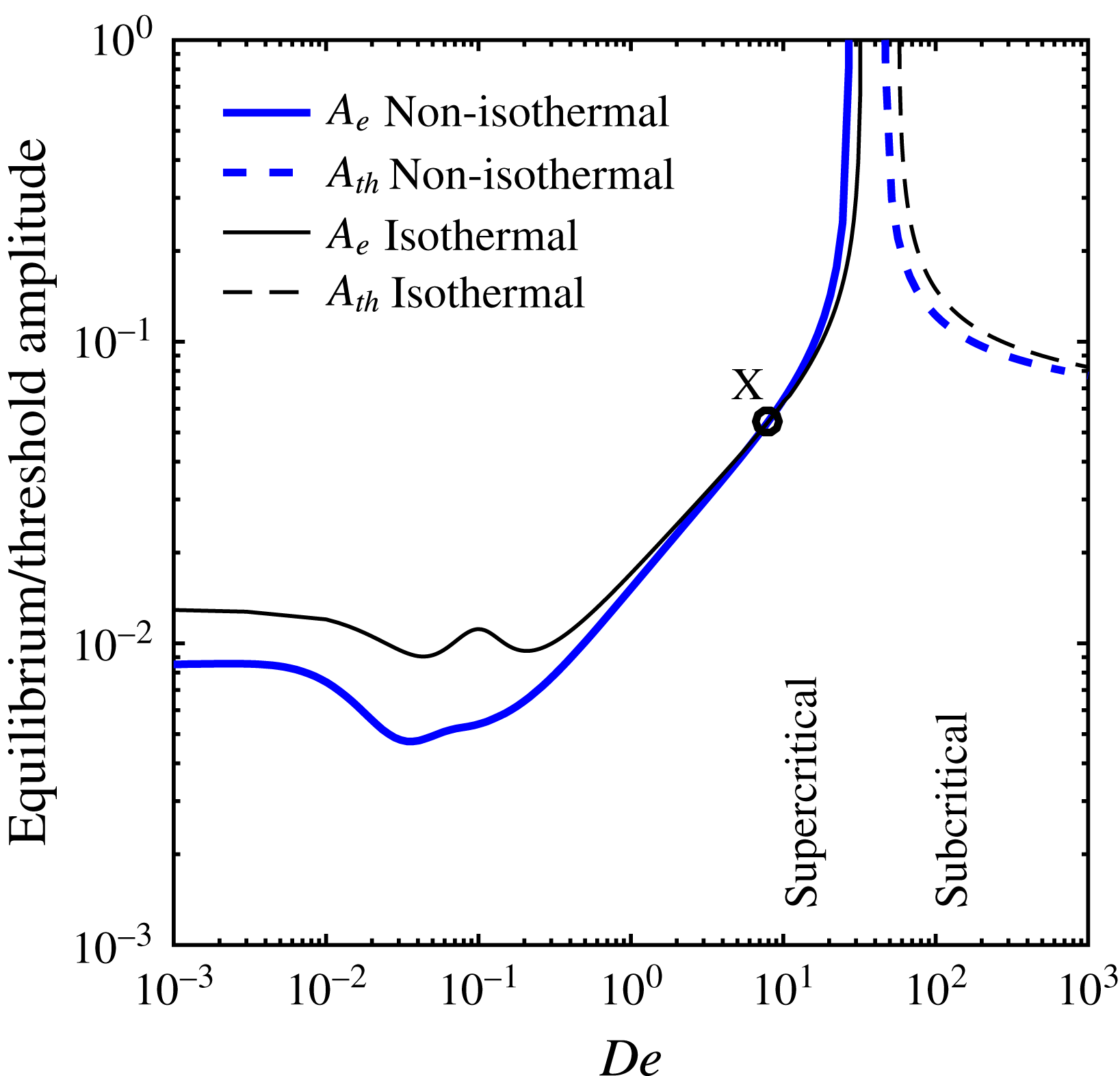
, the nonlinearities tend to stabilise the amplitude growth above the critical point (
 $DR>DR_{c}$
). In other words, the exponential growth of the disturbance amplitude is stabilised by nonlinear self-interaction of the fundamental mode to saturate the amplitude to an equilibrium value
 $A_{e}$
. Thus the flow is said to undergo a supercritical bifurcation at the critical point. On the contrary, for
 $l_{r}>0$
the nonlinearities tend to destabilise the flow, and it can become unstable even below the critical point (
 $DR<DR_{c}$
) provided the imposed disturbance amplitude is greater than a certain threshold value
 $A_{th}$
. Therefore, the finite amplitude manifold is of subcritical nature in the vicinity of the critical point.
The fixed point of amplitude equation (2.38), in the neighbourhood of
 $DR_{c}$
i.e.
 $s_{r}\sim O(A_{1}^{2})$
, gives an equilibrium amplitude from which the finite amplitude branch can be constructed. By setting the rate of change of amplitude to zero, the equilibrium or threshold amplitude is
 $$\begin{eqnarray}A=\sqrt{-s_{r}/l_{r}}.\end{eqnarray}$$
This relation should be the same for the equilibrium (supercritical branch) as well as the threshold amplitude (subcritical branch) since
 $s_{r}$
and
 $l_{r}$
are always of opposite signs in the region of interest.
3 Results and discussion
In the mathematical modelling § 2.1, the spinning fluid is considered to be ultra-high-molecular-weight polyethylene dissolved in decalin solvent. The material parameters for the UHMWPE–decalin system are given in table 2, where the values of the various dimensionless numbers appearing in the analysis are also listed. The values of the XPP parameters
 $r$
and
 $q$
are the same as those used in the earlier analyses for the same system (van der Walt et al.
Reference van der Walt, Hulsen, Bogaerds, Meijer and Bulters2012, Reference van der Walt, Hulsen, Bogaerds and Anderson2014; Gupta & Chokshi Reference Gupta and Chokshi2015, Reference Gupta and Chokshi2016). The XPP (
 $r$
and
 $q$
) and the rheological (
 $G_{0}$
and
 $\unicode[STIX]{x1D706}_{0}$
) parameters are in general obtained by rheology, i.e. transient extensional viscosity in a uniaxial extension experiment and linear oscillatory frequency sweep experiment respectively.
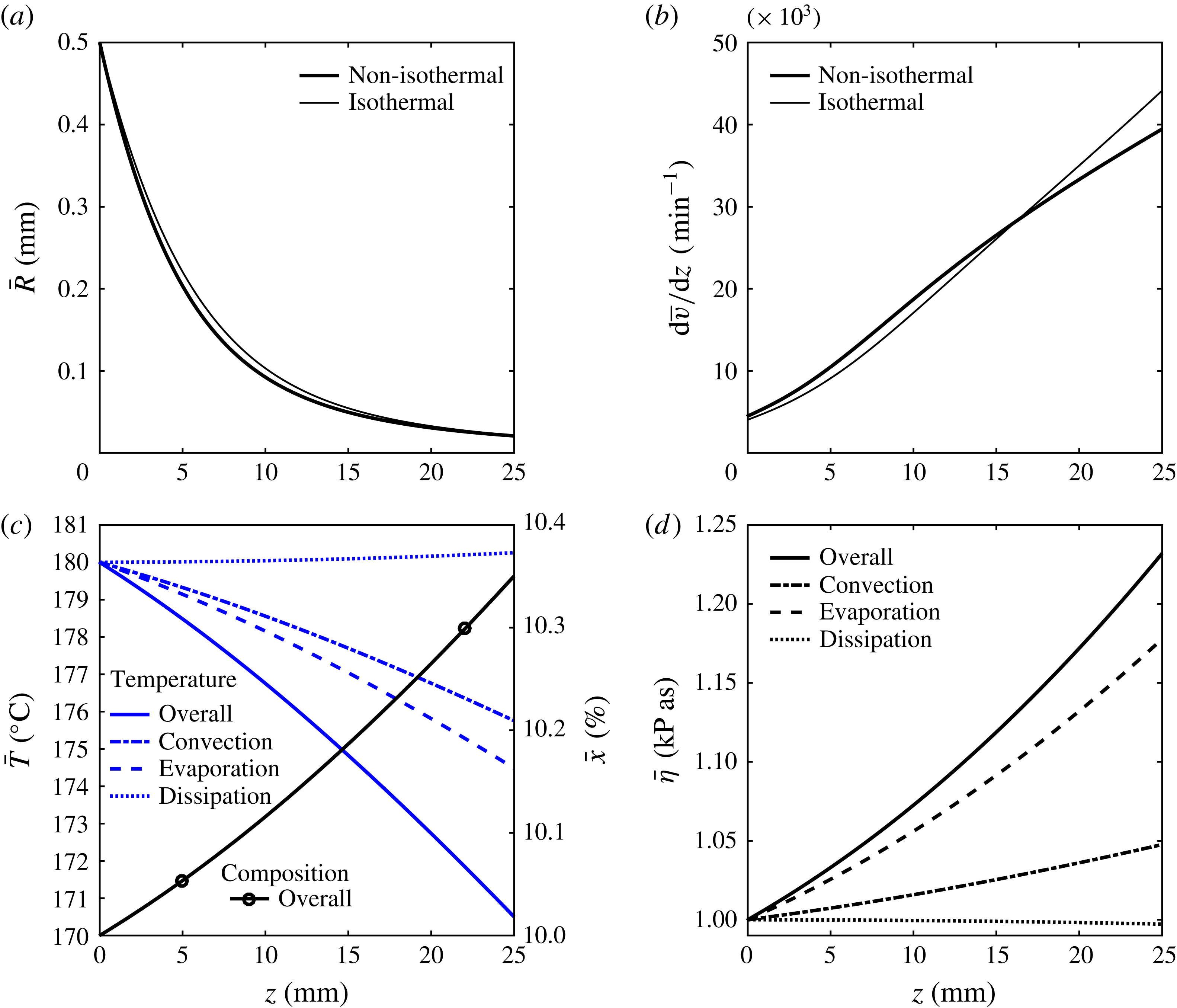
Steady-state profile of variables versus spinline coordinate
 $z$
. (a) Radius
 $R(z)$
, (b) local extension rate
 $\text{d}v/\text{d}z$
, (c) temperature
 $T(z)$
and polymer concentration
 $x(z)$
by wt.
 $\%$
and (d) local viscosity
 $\unicode[STIX]{x1D702}(z)$
. Comparison of non-isothermal (thick lines) with isothermal (thin solid lines) calculations exhibits the role of energy loss from the spinline. Temperature drop and rising polymer fraction contribute to viscosity enhancement, seen most by evaporation. Parameters:
 $De=0.1$
,
 $DR=23.18$
with other parameters specified in table 2.

3.1 Steady-state solution
For stability analysis, the steady-state solution forms the base state upon which the infinitesimally small and finite amplitude disturbances are imposed. The steady-state solution for the non-isothermal spinning flow is obtained by solving the governing equations (2.17)–(2.22) assuming zero time derivatives, by the shooting method. The steady-state profiles for fibre radius
 $R(z)$
, temperature
 $T(z)$
and polymer concentration
 $x(z)$
are shown in figure 2. In this figure, the variables are plotted in the dimensional form to appreciate the magnitude change due to non-isothermal effects. The spinning is accompanied by two non-isothermal effects. First, the material loss of solvent from the filament and the associated loss of latent heat appearing in the thermal energy conservation equation (2.20) (the term containing the mass Stanton number
 $St_{m}$
). Second, the loss of thermal energy by convective heat transfer to the surrounding air, indicated by the term containing heat Stanton number
 $St_{h}$
in the same equation. Thus, the radius, temperature and polymer mass fraction are directly influenced by the simultaneous heat and mass transfer, whereas the remaining spinline variables (velocity and stresses) are influenced indirectly due to the temperature and concentration dependence of the fluid viscosity. Comparison of non-isothermal (thick lines) with isothermal calculations (thin solid lines) shows the role of non-isothermal effects in the spinline variables. In figure 2(a), the evaporating solvent causes the radius to decrease. Figure 2(b) shows the strain rate along the fibre axis. Towards the end of spinline, the viscosity build-up by non-isothermal effects leads to a reduction in strain rate. Figure 2(c) shows the drop in the spinline temperature (thick solid line) as it proceeds from the spinneret to the take-up. Due to solvent evaporation, the polymer concentration increases along the flow direction, as shown in figure 2(c) (marked thick solid line). For an air gap of
 $25$
mm and the choice of parameters studied, the fibre temperature drops from
 $180\,^{\circ }$
C to nearly
 $170\,^{\circ }$
C and the polymer concentration increases from
 $10\,\%$
to around
 $10.35\,\%$
. The decreasing temperature and rising polymer concentration contribute to viscosity enhancement by nearly
 $50\,\%$
as shown in figure 2(d) (thick solid line). In figures 2(c) and 2(d), additional information (dash and dash-dot lines) about individual modes of heat transfer are shown, which will be discussed in § 3.2 in context.
3.1.1 Effect of spinline cooling on steady-state solution
In the governing equations (2.17)–(2.22), the energy balance equation (2.20) accommodates heat exchange of the spinline with the surroundings by three mechanisms – convection, evaporation and viscous dissipation. To understand the steady-state behaviour with increasing energy transfer, the convective mode is isolated by setting the mass Stanton number and the viscous dissipation to zero (
 $St_{m}=\unicode[STIX]{x1D6FC}=0$
) and increasing the thermal Stanton number. By increasing
 $St_{h}$
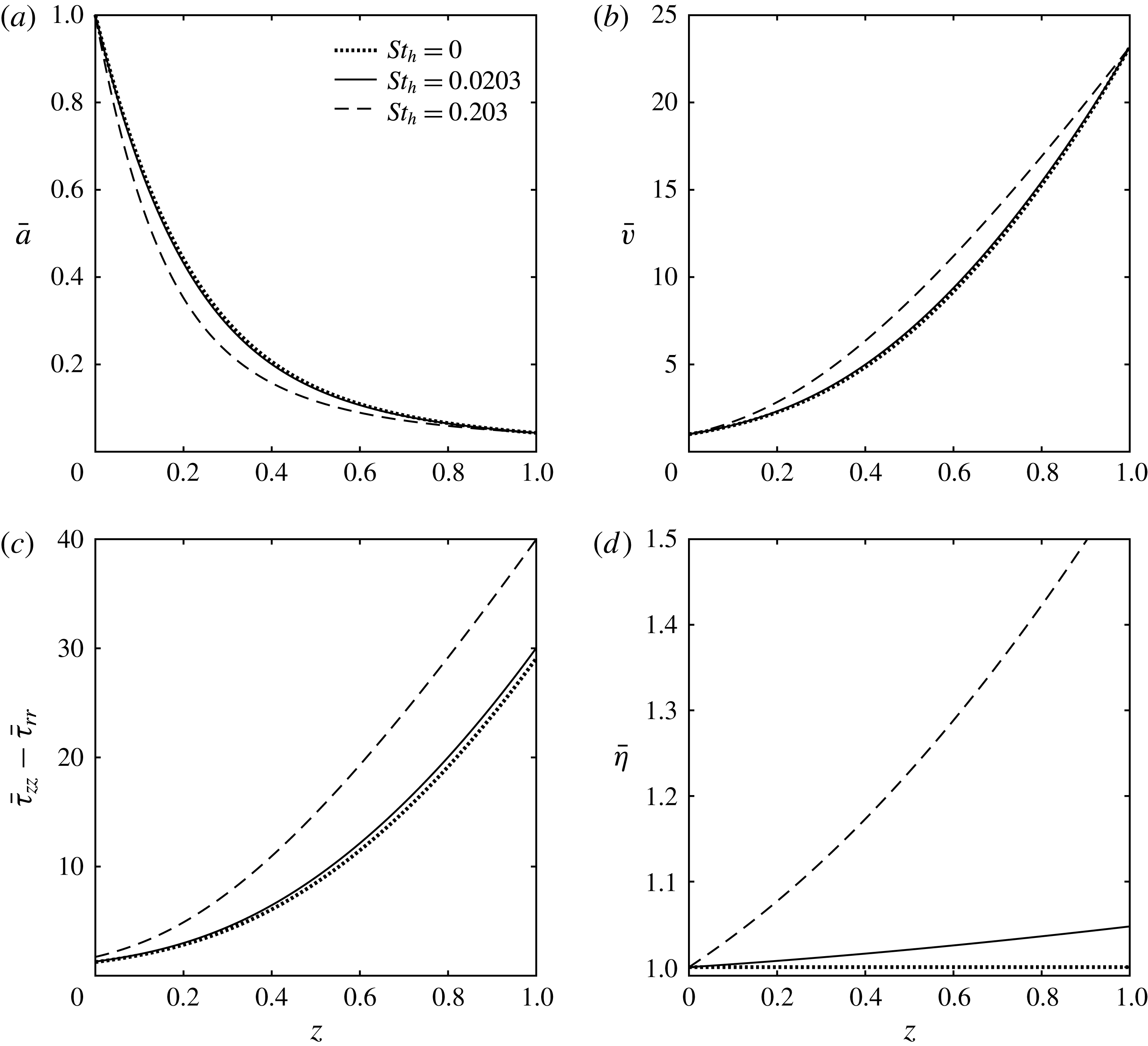
, the cooling of the spinline increases and the temperature across the spinline drops by a larger degree. The effect is that the spinline thins in between the fixed bounds of the spinneret and the take-up, as seen in figure 3(a). Since the area is coupled to the velocity by the mass conservation equation (2.17), figure 3(b) shows that the fibre speeds up between the fixed bounds of the spinneret and the take-up. Figure 3(b) qualitatively agrees with the results of Fisher & Denn (Reference Fisher and Denn1977), where the authors also report an enhancement of spinline velocity with increasing thermal Stanton number. This thinning and speeding up of the spinline occurs due to an increase in the spinline tension, as shown in figure 3(c), which is a consequence of the increasing stresses that are coupled to the spinline area in the momentum conservation equation (2.19). The higher stresses develop owing to an enhanced viscosity as shown in figure 3(d). In this plot, the local spinline viscosity scaled with respect to the initial condition
 $\bar{\unicode[STIX]{x1D702}}=\unicode[STIX]{x1D702}/\unicode[STIX]{x1D702}_{0}$
, increases due to the reduction in fibre temperature.
Steady-state plots of (a) spinline area, (b) spinline velocity, (c) first normal stress difference and (d) viscosity along the spinline length
 $z$
, compared for increasing thermal Stanton number. Parameters are specified in table 2.

3.2 Linear stability analysis
For infinitesimally small amplitude disturbances, the linear stability analysis predicts the critical draw ratio
 $DR_{c}$
for the onset of draw resonance instability by setting the real part of the complex growth rate
 $s_{r}$
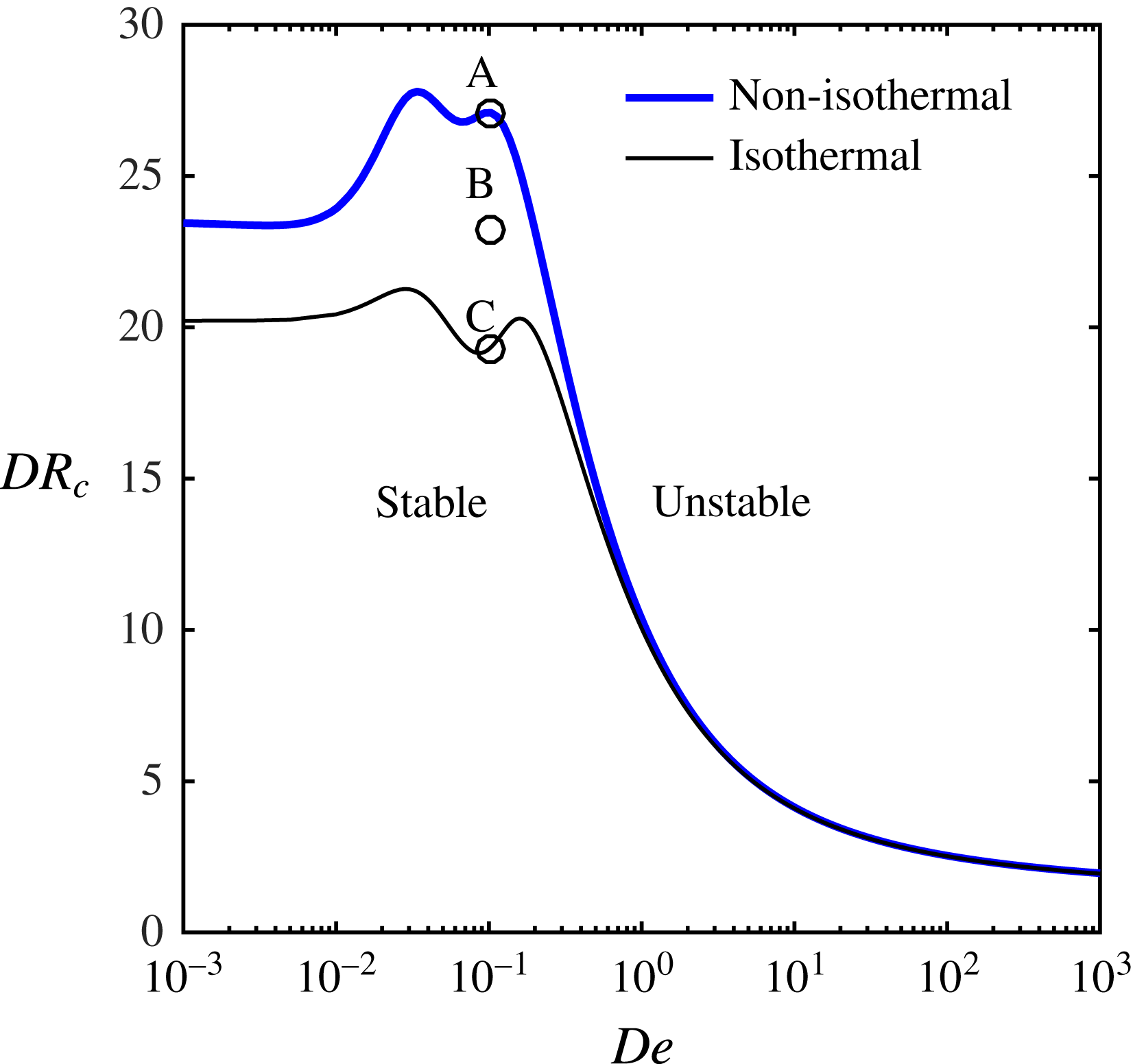
to zero. The variation of
 $DR_{c}$
with flow Deborah number
 $De$
results in the stability map shown in figure 4. The neutral stability curve for the isothermal spinning (thin line) is same as that reported in earlier analyses (van der Walt et al.
Reference van der Walt, Hulsen, Bogaerds, Meijer and Bulters2012; Gupta & Chokshi Reference Gupta and Chokshi2015), and is shown for comparison with the neutral stability curve for the non-isothermal spinning (thick line). The region below the curve (
 $DR<DR_{c}$
) indicates stable spinning, while above the curve (
 $DR>DR_{c}$
) represents spinning with draw resonance instability. In the limit
 $De\rightarrow 0$
, the fluid behaves like a Newtonian fluid, as the polymer chains are not deformed from their globular state. As the viscoelasticity of the flow increases with Deborah number
 $De$
, the chains are increasingly in an oriented and stretched state. The linear viscoelastic model behaviour continues till
 $De\approx 10^{-2}$
, where the backbone stretch ratio
 $\unicode[STIX]{x1D6EC}\approx 1$
. In this regime, only the backbone orientation relaxation time is of significance (Verbeeten et al.
Reference Verbeeten, Peters and Baaijens2001). On the other hand, for highly stretched flow in the range
 $De>1$
,
 $\unicode[STIX]{x1D6EC}\gg 1$
, which means that only the backbone stretch relaxation time is of significance. Thus, in the interim
 $10^{-2}<De<1$
range, the variation of
 $DR_{c}$
with
 $De$
shows two peaks corresponding to two relaxation time scales associated with the polymer chain. The separation of peaks is related to the separation of these two relaxation times given by their ratio, the parameter
 $r$
, such that
 $r\geqslant 1$
.
Variation in critical draw ratio
 $DR_{c}$
, with flow Deborah number
 $De$
. The region below the neutral stability curve indicates stable flow, and that above it represents the linearly unstable flow. The figure compares obtained curves under non-isothermal and isothermal conditions to highlight the role of energy loss on stability. At points marked A, B and C, the growth rate eigenspectra are constructed, as shown in figures 6 and 7, discussed later. Parameters are specified in table 2.

Around the range of Deborah numbers approaching the first peak, the backbone chains undergo orientation in the deformation direction. This orientation is resisted by the neighbouring chains, leading to a viscosity build up that manifests in a peaked
 $DR_{c}$
value. With increasing viscoelasticity of the flow, these constraints (neighbouring chains) relax to some degree allowing chain orientation, causing the extensional viscosity thinning behaviour. This thinning behaviour manifests in the form of decreasing
 $DR_{c}$
value. These nearly oriented backbone chains then begin to undergo stretching caused by the presence of dangling arms at each branch point of the chain. The backbone chain stretching leads to viscosity build up indicated by the second peak in
 $DR_{c}$
value. In the limit of high elasticity post second peak, dangling arms at the branch points retract to the branch point releasing the stretch build up and allowing the backbone chain to reptate. Thus, for fast extensional flows, the XPP fluid exhibits an extensional softening effect achieved by reptation motion of the polymeric chains (Gupta & Chokshi Reference Gupta and Chokshi2015). The strain softening leads to destabilisation, indicated by a decrease in
 $DR_{c}$
with
 $De$
.
In the limit of a Newtonian fluid, the value of the critical draw ratio for non-isothermal spinning is significantly higher than 20.218, the corresponding value for isothermal spinning. This additional stabilisation was found for viscoelastic fluids as well, though the additional stability decreases for strongly viscoelastic flows (
 $De\gg 1$
). The stabilising role of non-isothermal effects is attributed to non-uniform temperature and concentration dependent viscosity along the fibre realised by spinline cooling. The additional stability for a viscoelastic fluid stems from the reduced mobility of the polymeric chain suppressing the relaxation of stretch in the backbone of the polymer molecule (Peterlin Reference Peterlin1974). The slowdown of polymer chain relaxation mechanisms due to cooling, given by the dependence of relaxation time on the temperature in (2.10), means that the apparent Deborah number
 $\unicode[STIX]{x1D706}v_{0}/L$
is larger than the Deborah number based on conditions at the die-exit point
 $De=\unicode[STIX]{x1D706}_{0}v_{0}/L$
. This difference in
 $De$
is reflected as a slight horizontal shift of the peaks of the neutral stability curve towards the left side when the spinline cooling is taken into account. For highly elastic flows in the limit
 $De\gg 1$
, the destabilisation by the extensional thinning effect is dominant over the stabilisation by cooling of the spinline. Thus, the isothermal and non-isothermal neutral stability curves tend to meet for highly viscoelastic flows.
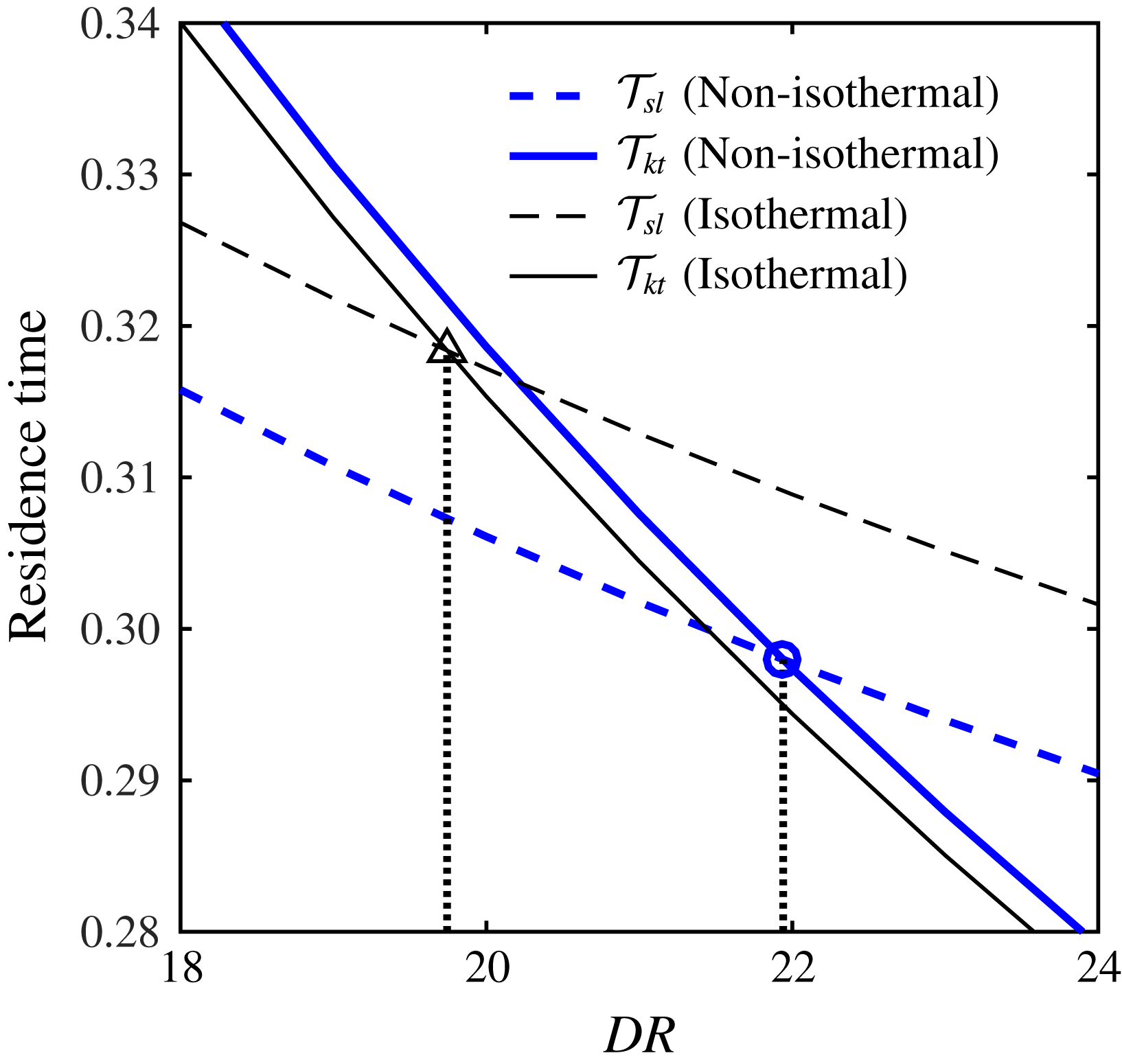
Residence times of the spinline
 ${\mathcal{T}}_{sl}$
and a cycle of kinematic throughput wave
 ${\mathcal{T}}_{kt}$
, against the draw ratio
 $DR$
for Newtonian fibre spinning, although the mechanism extends to viscoelastic flows as well. The two residence times meet at a draw ratio
 $DR_{c}=19.77$
for isothermal spinning (▵), and
 $DR_{c}=21.96$
for non-isothermal spinning (○). Parameters are specified in table 2.

The instability can also be understood kinematically as the sustained progression of a throughput (volumetric flow rate) disturbance wave as suggested by Hyun (Reference Hyun1978). When the time period of one cycle of throughput wave
 ${\mathcal{T}}_{kt}$
is less than the fluid residence time during spinning
 ${\mathcal{T}}_{sl}$
, the disturbances decay and the flow is termed stable. However, when
 ${\mathcal{T}}_{kt}>{\mathcal{T}}_{sl}$
, the travelling wave becomes sustainable, and the draw resonance occurs. For neutral stability at
 $DR=DR_{c}$
, the time period of the kinematic throughput wave is equal to the spinline residence time
 ${\mathcal{T}}_{kt}={\mathcal{T}}_{sl}$
. To comprehend the draw resonance for non-isothermal spinning, a numerical estimation of the two time scales for different values of draw ratio is done. The comparison of the residence times of the spinline
 ${\mathcal{T}}_{sl}$
and that of a cycle of a throughput kinematic wave
 ${\mathcal{T}}_{kt}$
, for an isothermal and a non-isothermal spinline is shown in figure 5. For a spinline that loses both thermal energy and solvent, it is observed that a throughput wave takes longer to pass the spinline length, whereas the fluid residence time reduces greatly in comparison to isothermal spinning. Both these factors contribute to the postponement of draw resonance indicated by an increase of
 $DR_{c}$
, though the latter is clearly more dominant. It must be noted that the
 $DR_{c}$
prediction by the kinematic theory is in close agreement with the results of linear stability.
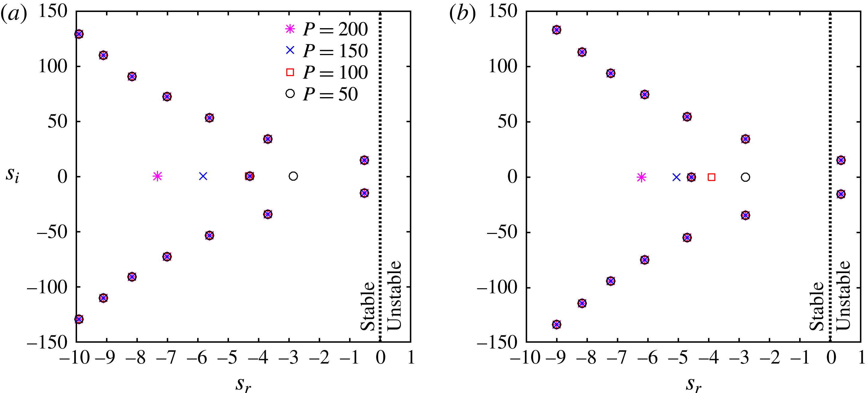
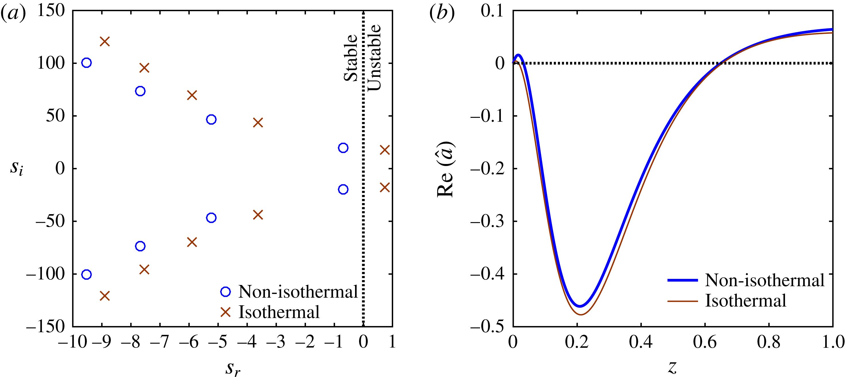
Eigenspectrum for complex-valued linear growth rate
 $s$
calculated in (a)
 $-5\,\%$
, and (b)
 $+5\,\%$
vicinity of
 $DR$
corresponding to point A in figure 4. The physical eigenmodes are independent of the number of Chebyshev collocation points
 $P$
. The leading mode is negative when
 $DR<DR_{c}$
and positive when
 $DR>DR_{c}$
. Hence the two methods (spectral and shooting) predict the same
 $DR_{c}$
. Parameters are specified in table 2.

The stability diagram in figure 4 is constructed using the shooting method which numerically estimates the largest growth
 $s=s_{r}+\text{i}s_{i}$
for a given draw ratio
 $DR$
. At the critical point
 $DR=DR_{c}$
, the real part
 $s_{r}$
is set to zero. While the shooting method predicts only the leading eigenmode, the Chebyshev collocation technique using
 $P$
collocation points is used to construct the entire eigenspectrum of disturbance growth rates. The eigenspectra are generated in approximately a
 $\pm 5\,\%~DR$
range of point A on the neutral stability curve of figure 4. In figure 6(a), for
 $DR\lesssim DR_{c}$
the spectrum has a leading mode pair with a small negative real part
 $s_{r}\approx -0.2$
. The negative sign implies that the spinning flow is linearly stable with no other mode dominating the flow. Similarly, in figure 6(b) for
 $DR\gtrsim DR_{c}$
, the leading pair of eigenmodes has a small positive part
 $s_{r}\approx 0.2$
indicating linearly unstable flow. Here, all the eigenvalues except those with
 $s_{i}=0$
are found to be independent of the number of collocation points
 $P$
. It should be noted that the leading mode found by the spectral method is the same as the linear growth rate
 $s$
that is predicted by the shooting method.

In figure 7(a), a comparison of the eigenspectra is presented for isothermal and non-isothermal spinning at point B on the neutral stability curve of figure 4. At this point, the isothermal spinning is linearly unstable which is confirmed by the positive value of
 $s_{r}$
for the leading pair of eigenmodes. However, for non-isothermal spinning, the leading pair of growth rates becomes negative indicating stable spinning flow. The non-zero imaginary component of leading mode
 $s_{i}$
indicates a wave-like progression of disturbance through the spinline, and the value of
 $s_{i}$
denotes the frequency of oscillations. The shape of the disturbance area profile, the eigenfunction corresponding to the leading mode, is shown in figure 7(b) for both isothermal and non-isothermal cases. It is this disturbance in fibre area that oscillates due to non-zero imaginary part
 $s_{i}$
giving rise to, in a material frame of reference, a travelling wave of disturbance superimposed on the steady-state fibre profile. Upon comparing the frequencies of the leading mode instability in isothermal (
 $s_{i}=18.18$
) and non-isothermal (
 $s_{i}=19.24$
) spinlines, it can be inferred that spinline cooling accelerates travel of the disturbance waves. It is found that at any point along the neutral stability curves in figure 4, the imaginary part of linear growth rate
 $s_{i}$
is higher for the non-isothermal spinning than its value for the isothermal spinning at the same Deborah number. This fast travelling of perturbations in an non-isothermal spinline, when compared to an isothermal one, occurs due to faster transmission of the perturbation energy along the uniform long-range macromolecular network, which is under larger stress when compared to relatively non-uniform chain network of the isothermal case (Jung et al.
Reference Jung, Song and Hyun1999). The larger stress in a uniform network translates to a rather quick change of spinline variables, resulting in a shorter time period of the waves.
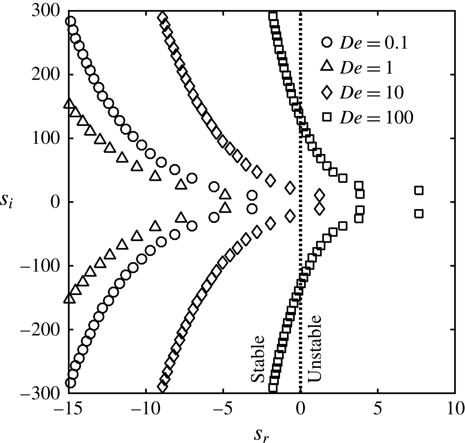
Variation of non-isothermal eigenspectra with increasing
 $De$
for
 $DR=5$
. As
 $De$
rises from the Newtonian limit, the spectrum indicates stabilising flow (negative
 $s_{r}$
shift), followed by rapid destabilisation (positive
 $s_{r}$
shift). The lowest magnitude non-zero frequency mode remains the leading mode for any
 $De$
. Parameters are specified in table 2.

Figure 8 shows the variation in the eigenspectrum with flow Deborah number at a fixed draw ratio
 $DR=5$
to ensure that no other dominant mode characterises the flow other than the one predicted by the shooting method. For
 $De=0.1$
, the leading mode of the spectrum lies well within the stable limit as
 $DR<DR_{c}$
. As
 $De$
is increased, the spectrum shifts in the negative
 $s_{r}$
direction, indicating the stabilising role of fluid elasticity due to extensional hardening. Upon further increasing
 $De$
, the region of rapid destabilisation begins, thus the spectrum advances in the positive
 $s_{r}$
direction. At
 $De=100$
, modes other than the leading pair are also seen in the unstable regime too, suggesting a strongly destabilised flow, since the chosen
 $DR=5$
is greater than the critical value. Importantly, for the entire range of Deborah numbers, the mode with the smallest magnitude non-zero imaginary part
 $s_{i}$
remains the leading mode, the one with the largest value of the real part
 $s_{r}$
.
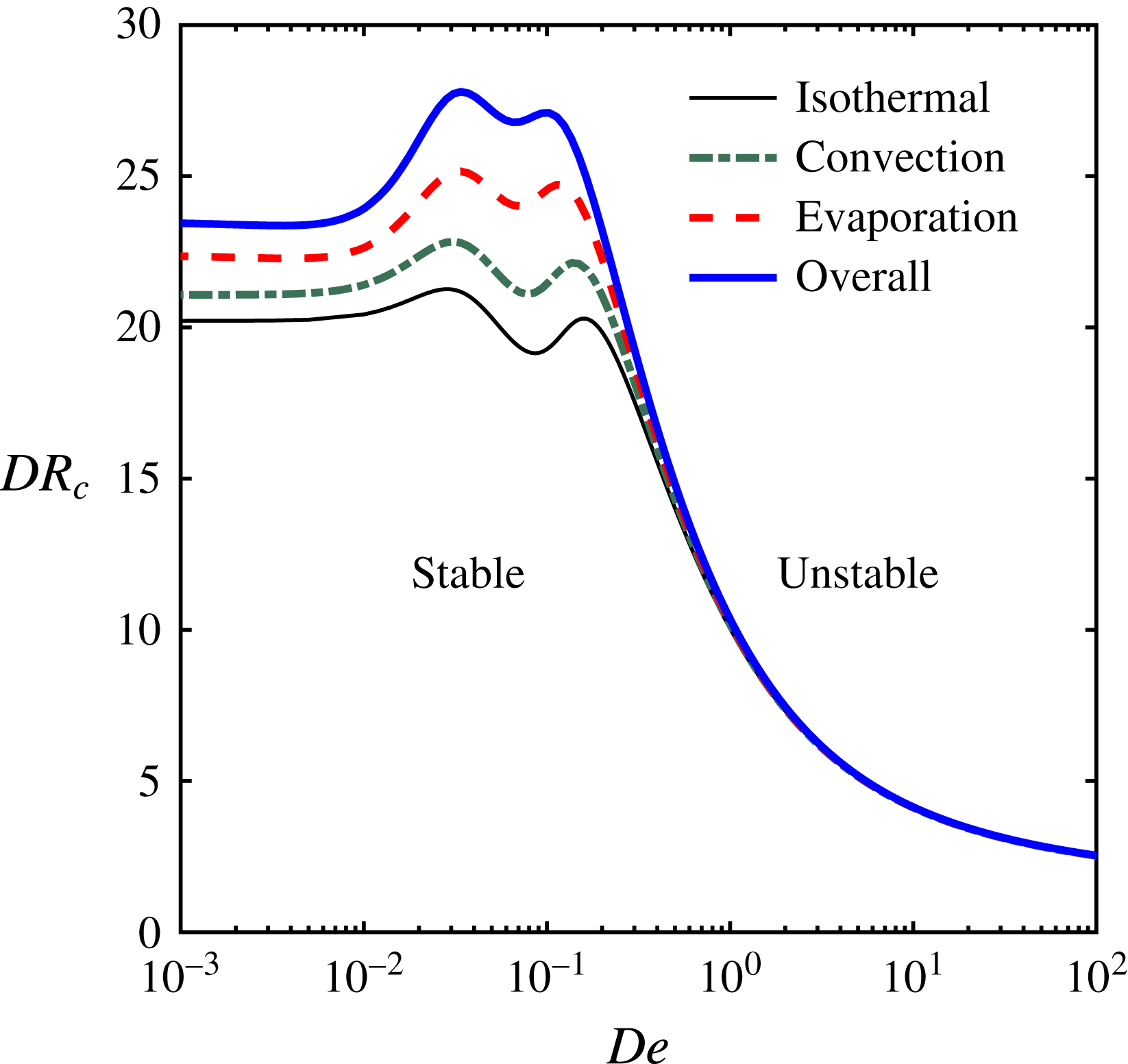
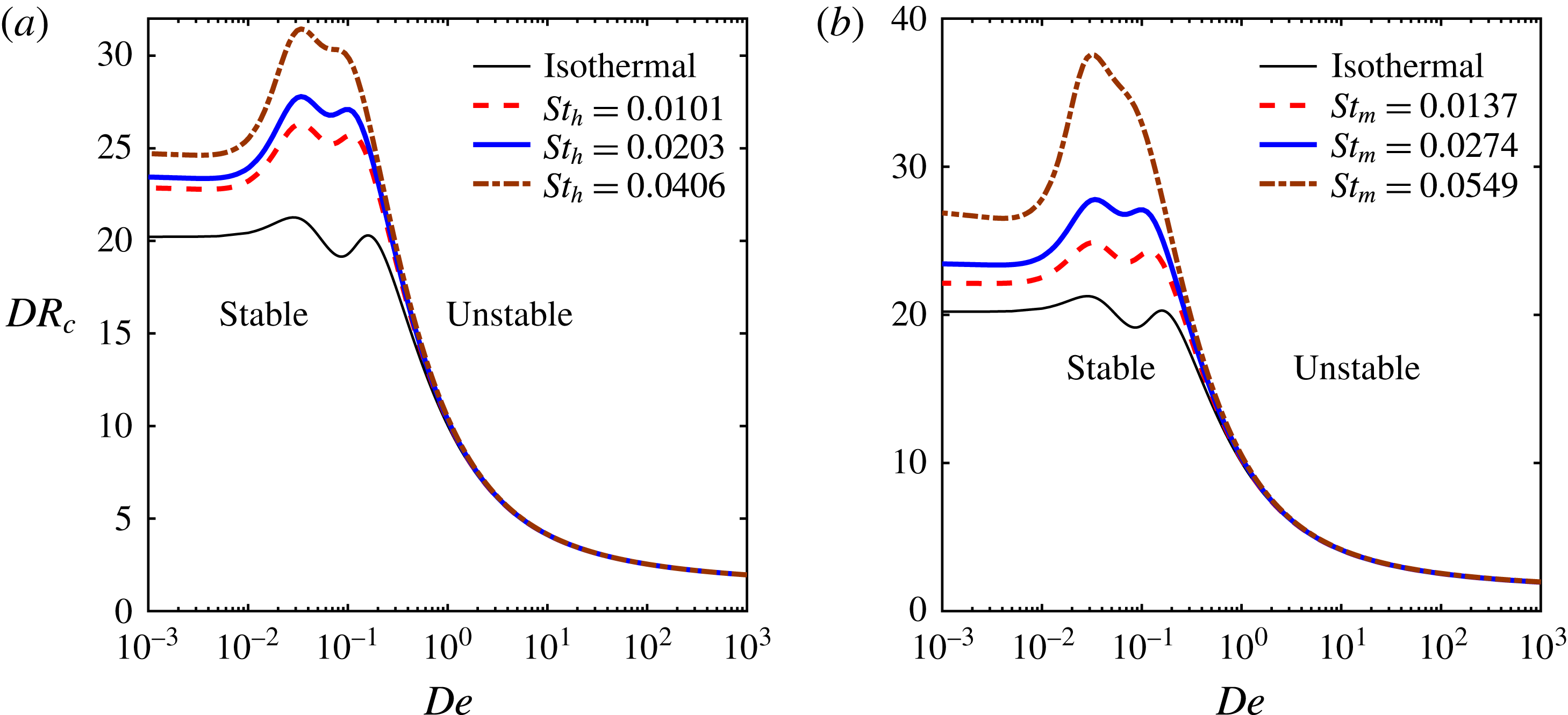
Variation in the critical draw ratio
 $DR_{c}$
with flow Deborah number
 $De$
. The individual roles of two non-isothermal mechanisms, i.e. pure convection and pure solvent evaporation to ambient air are seen. The contribution from evaporation is found to be stronger than that from only convection. Spinning parameters are specified in table 2.

Next, the role of individual heat loss mechanisms in the enhancement of spinline stability is shown in figure 9. The dash-dot line represents the neutral stability curve considering the convective heat transfer as the only non-isothermal effect, with the solvent evaporation and viscous dissipation terms being disabled. This case can be seen as a non-isothermal melt spinning process. The dashed line represents the neutral stability curve calculated with the convection and viscous dissipation terms disabled, i.e. the spinline loses heat by only solvent evaporation mode. This case can be seen as a non-isothermal solution spinning process without convection to ambient air. Both the convection and solvent evaporation mechanisms individually tend to play a stabilising role due to rheology modification upon cooling. In qualitative validation of the finding of the stability analysis, the experimental study by Demay & Agassant (Reference Demay and Agassant1985) reports the stabilising role of heat convection on polyester fibre spinning, in which the critical
 $DR$
increases with increasing the heat Stanton number. Interestingly, the vertical shift of the neutral stability curve is found to be more pronounced for the solvent evaporation mechanism in comparison to the convection mode. The solvent evaporation enhances viscosity by not only temperature drop associated with evaporative cooling but also by enrichment of polymer concentration in the fibre. In the steady-state profiles in figure 2(c,d), the temperature drop and viscosity enhancement by both these mechanisms are compared. While pure convection increases the viscosity by only
 $10\,\%$
, pure evaporation tends to increase viscosity by nearly
 $40\,\%$
due to a greater temperature drop by latent heat removal. The solely viscous dissipation, which tends to increase the fibre temperature, leads to only a marginal reduction in viscosity. Thus, its influence on the neutral stability curve is insignificant. To summarise, the solvent evaporation mode of heat transfer plays a more important role in stability behaviour than the convective heat transfer and the onset of draw resonance can be delayed significantly by factors enhancing solvent removal during spinning.
The cooling of the spinline enhances the extensional viscosity by restricting the chain relaxation mechanisms. For convection and evaporation mechanisms, this viscosity enhancement has to be differentiated, to understand figure 9 in a better way. Topological homogenisation of entanglements is more favourable for the drawability of high-molecular-weight polymers (Smith & Lemstra Reference Smith and Lemstra1979). With pure melts, the entanglements between macromolecules, or the ‘friction points’ remain high but are localised, may be discontinuous and hence the overall integrity of the structure contains defects which may lead to instabilities under fast extensional flow. For polymer solution, with the addition of a diluent, a tenuous structure of somewhat fewer entanglements is achieved although with fewer defects, such that a rigid long-range entanglement network of molecules is formed. Now, when cooling happens, the relaxation of polymeric chains is restricted, thus offering more extensional viscosity. Additionally, the evaporating solvent also reduces chain mobility by creating new friction points as solvent particles leave the system. Thus even though stability increases by convection for pure melt spinning, the enhancement is still less when compared to broadening of the stable region by evaporation for solution spinning.
The stability of the spinning flow is sensitive to various process parameters. The two dominant factors that affect both convection and evaporation are cross-air velocity
 $v_{a}$
and material activation energy
 $E$
. As explained earlier in § 2,
 $v_{a}=0$
refers to parallel co-current flow of cooling air, and as
 $v_{a}$
increases, the air flow is increasingly cross-current. Since the cross-current flow tends to withdraw heat and mass more efficiently, an enhancement in stability is expected as cross-flow increases. In the governing equations (2.17)–(2.22), the function
 $\unicode[STIX]{x1D713}(a,v,v_{a})$
affects both convection and evaporation terms. Figure 10(a) depicts the effect of cross-flow air velocity
 $v_{a}$
(made dimensionless using the extrusion velocity
 $v_{0}$
) on the stability diagram. As cooling air speed increases, the critical draw ratio
 $DR_{c}$
increases significantly for low to moderate values of flow Deborah number. Noticeably, amongst the two peaks, the first one related to the longest relaxation time is significantly affected by the cooling. This effect is attributed to a slowdown in chain relaxation due to reduced mobility. For highly elastic fluids in the limit of
 $De\gg 1$
, the extensional softening is far more dominant than the cooling induced hardening, implying an insignificant role of non-isothermal effects. This behaviour will be common to all the subsequent parametric variations. In an experimental study by Kase (Reference Kase1974) investigating draw resonance in a water quenched melt spinning of polyethylene terephthalate (PET), the author exhibits stabilisation by increasing the cooling cross-air velocity. For gel/solution spinning, additives in high concentration (
 $1\,\%$
by wt.) can cause the material activation energy to increase by nearly
 $100\,\%$
, subsequently suppressing the spinning instabilities by making decalin a poorer solvent to UHMWPE such that polymer–polymer interactions dominate and more entanglements are created (Yang & Chen Reference Yang and Chen1997). Further, the higher the activation energy is, the greater the fluid viscosity sensitivity to the temperature variation will be. This effect is depicted in figure 10(b), where the increase in activation energy tends to broaden the region for stable spinning.
Variation in critical draw ratio with flow Deborah number
 $De$
, for varying (a) cross-flow air velocity
 $v_{a}$
, and (b) activation energy
 $E$
. When
 $v_{a}=0$
, the cooling air is co-current, and increasingly becomes cross-current as
 $v_{a}\rightarrow \infty$
. The stability is sensitive to cooling air velocity and its orientation, and also to material activation
 $E$
. Other spinning parameters are specified in table 2.

There may exist changes in certain parameters that only affect either one or the other cooling mechanism. For example, if ambient temperature
 $T_{a}$
were to be maintained at a lower temperature, the convection mode would be promoted with no effect on evaporation; whereas evaporation could be promoted by choosing a diluent with high volatility, in which case convection would be constant. It would be convenient to study such effects via the variation of thermal and mass Stanton numbers
 $St_{h}$
and
 $St_{m}$
. The variation of
 $St_{h}$
and
 $St_{m}$
from half to double the values calculated from the parameters in table 2 is shown in figure 11. Figure 11(a) shows only a minor change to the non-isothermal neutral stability curve by variation of
 $St_{h}$
, while figure 11(b) shows a major change to the non-isothermal neutral stability curve by variation of
 $St_{m}$
. Thus stability enhancement by spinline cooling is found to be more sensitive to the evaporation mode than the convection mode.
Variation in critical draw ratio with flow Deborah number
 $De$
, for varying (a) thermal Stanton number
 $St_{h}$
, and (b) mass Stanton number
 $St_{m}$
. The spinline is more sensitive to changes
 $St_{m}$
than
 $St_{h}$
. Parameters are specified in table 2, other than varying
 $St_{h}$
for (a) and
 $St_{m}$
for (b).

Finally, it would also be interesting to examine the effect of material rheology on the stability behaviour. It is known that real polymers of interest to high-strength fibre spinning exhibit extensive strain hardening effect for a range of strain rates. This effect is captured by increasing the value of the XPP parameter
 $q$
, which denotes the number of arms at each branch point. Increasing
 $q$
leads to stronger stretching of the backbone chain until retraction of the dangling arms to the branch point, a necessity for the backbone chain to relax by reptation. In short,
 $q$
is a measure of the degree of branching in the polymer which is responsible for extensional hardening, making the material suitable for spinning. The effect of the strain hardening parameter
 $q$
on the stability diagram is shown in figure 12(a). It is seen that the neutral stability curve is enhanced to greater values of
 $DR_{c}$
indicating the stabilising role of the strain hardening parameter. It should be noted that this stabilisation by an increasing degree of branching is greater under non-isothermal conditions. This effect is mainly due to an increased friction coefficient by cooling which results in greater resistance to arm retraction to the branch point leading to enhanced strain hardening effect. Another rheological parameter in the XPP model is
 $r$
, the ratio of backbone orientation to stretch relaxation times. The influence of
 $r$
on the stability diagram is shown in figure 12(b). Increasing the parameter
 $r$
implies increased separation of the two chain relaxation modes which leads to increased separation between the two peaks in the stability map. The stabilising role of non-isothermal spinning is visible for any choice of rheological parameters.
Variation in critical draw ratio with flow Deborah number
 $De$
, for varying XPP parameters: (a) the strain hardening parameter
 $q$
, and (b) the chain orientation to stretch relaxation time ratio
 $r$
. Spinning parameters are specified in table 2, other than varying
 $q$
for (a) and
 $r$
for (b).

3.3 Weakly nonlinear analysis
The linear stability theory predicts the onset of draw resonance in terms of
 $DR_{c}$
such that the infinitesimally small amplitude disturbances grow exponentially in the unstable region with
 $DR>DR_{c}$
. In reality, beyond the critical point, the growing disturbance amplitude saturates because of the stabilising role of nonlinearities ignored in the linear stability analysis (for supercritical bifurcation at the critical point). The equilibrium amplitude represents the amplitude of the periodic oscillations in the fibre cross-sectional area when the draw resonance sets in. In case of a destabilising role of nonlinearities, the spinning flow can become unstable even in the linearly stable region (
 $DR<DR_{c}$
) when perturbed with disturbances of finite amplitude (for subcritical bifurcation at the critical point). Thus, for finite amplitude disturbances, the role of nonlinearities in the governing equations (2.17)–(2.22) needs to be investigated to determine the nature of bifurcation at the critical point. Weakly nonlinear stability analysis is thus employed to consider the dynamics of finite amplitude disturbances as governed by the Landau equation (2.40). In this equation, the higher-order correction to the linear growth rate is obtained as the complex-valued Landau constant
 $l=l_{r}+\text{i}l_{i}$
, whose real part
 $l_{r}$
provides the
 $O(A_{0}^{2})$
correction to the linear growth rate
 $s_{r}$
. The imaginary part
 $l_{i}$
accounts for the
 $O(A_{0}^{2})$
correction to the linear frequency
 $s_{i}$
. The weakly nonlinear analysis is valid in the vicinity of the critical point such that
 $|DR-DR_{c}|\sim O(A_{0}^{2})$
.
Variation in the real part of the Landau constant
 $l_{r}$
with flow Deborah number
 $De$
calculated along the neutral stability curve in figure 4. Both isothermal (thin line) and non-isothermal (thick line) spinning are considered for comparison. Spinning parameters are specified in table 2.

The nonlinear correction to the growth rate
 $l_{r}$
is calculated at all points along the neutral stability curve in figure 4. The variation in the real part of the Landau constant
 $l_{r}$
with flow Deborah number is shown in figure 13. The results for the isothermal case are also shown for comparison. For low to moderate
 $De$
, the nonlinear growth rate is found to be negative, indicating the stabilising role of the nonlinearities in the problem giving rise to a supercritical Hopf bifurcation at the critical point. While being negative, the magnitude of
 $l_{r}$
is found to be much greater for the non-isothermal spinning than for the isothermal spinning. Thus, the non-isothermal effects related to viscosity enhancement upon cooling and solvent evaporation exhibit a stabilising influence on the finite amplitude stability behaviour. The stabilising effect of nonlinearities is maximum at a Deborah number corresponding to the extensional hardening peak in the linear stability diagram of figure 4. Upon increasing
 $De$
further, the extensional softening tends to reduce the magnitude of
 $l_{r}$
as it approaches zero and finally changes the sign to positive for highly elastic fast flows in the limit
 $De\gg 1$
. Thus, the nature of finite amplitude bifurcation crosses over from supercritical stable state to subcritical unstable state. It is found that the crossover Deborah number is slightly lower for the non-isothermal spinning (
 $De\approx 35$
) than for the isothermal spinline (
 $De\approx 42$
).
The finite amplitude manifold, in terms of equilibrium or threshold amplitude, plotted against the deviation of draw ratio from its critical value. The finite amplitude branches signify Hopf bifurcation at the critical point. (a) Effect of fluid elasticity is to reduce the equilibrium amplitude of the supercritical bifurcation; (b) increasing
 $De$
beyond a limit (strain hardening peak) tends to increase the equilibrium amplitude; and (c) for highly elastic fluids undergoing fast flows, the bifurcation crosses over to the subcritical state at
 $De\approx 35$
. Parameters are specified in table 2.

With the help of the Landau constant, the equilibrium amplitude is calculated as the fixed point of the dynamical Landau equation (2.41). This calculation allows us to construct a finite amplitude manifold emerging from the critical point
 $DR=DR_{c}$
. In figure 14, the equilibrium amplitude is plotted against the deviation from the critical point
 $(DR-DR_{c})$
for different values of Deborah number. For
 $0.001<De<0.05$
, figure 14(a) shows that the equilibrium amplitude of the draw resonance decreases upon increasing
 $De$
. In this regime, the stabilising extensional hardening effect is responsible for the reduction in the severity of draw resonance. The maximum stabilisation occurs at
 $De\approx 0.05$
around which point the magnitude of the negative nonlinear growth
 $l_{r}$
is maximum. Upon increasing
 $De$
, the trend reverses and the equilibrium amplitude increases with
 $De$
as shown in figure 14(b), indicating increasing severity of draw resonance as fluid elasticity increases. The magnitude of the nonlinear growth rate
 $l_{r}$
decreases with the sign remaining negative. For highly elastic flows with
 $De\gg 1$
, the sign of
 $l_{r}$
changes from negative to positive resulting in a bifurcation that crosses over from the supercritical state to the subcritical state, as illustrated in figure 14(c). For subcritical bifurcation, the fixed point amplitude of the Landau equation given by (2.41) represents the threshold amplitude such that disturbances of amplitude greater than the threshold value render the flow unstable even for
 $DR<DR_{c}$
. Figure 14(c) clearly shows the crossover of bifurcation as the finite amplitude manifold turns backwards on increasing
 $De$
beyond the crossover value of approximately 35. Any further increase in
 $De$
lowers the threshold amplitude of the subcritical manifold implying that the spinning flow becomes increasingly prone to destabilisation by even smaller amplitude disturbances despite the flow being linearly stable for
 $DR<DR_{c}$
. As the subcritical manifold is an unstable branch, practically, the spinning operation in this regime may lead to breakage of fibre.
Interestingly, all these branches lay lower than those for the isothermal case studied in Gupta & Chokshi (Reference Gupta and Chokshi2015). For the supercritical bifurcation regime, this implies that the amplitude of the periodic oscillations post-draw resonance is weaker (meaning less severe draw resonance) for non-isothermal spinning in comparison to the equivalent isothermal case. This fact has been verified by full numerical transient simulations as well, and is explained in the supplementary material. However, in the regime of the subcritical state (fast flows of highly elastic fluids), the threshold amplitude to excite an instability is lower for the non-isothermal flow than for the isothermal flow. Thus, the nonlinear stabilisation by spinline cooling decreases as
 $De$
increases, and cooling effect becomes nonlinearly destabilising at very high
 $De$
. Figure 15 plots the equilibrium/threshold amplitude, calculated from (2.41), in the vicinity of
 $DR_{c}$
(1
 $\,\%$
deviation from
 $DR_{c}$
) for a range of flow Deborah number. It is seen that for
 $De<8$
, cooling and solvent evaporation weakens the intensity of draw resonance amplitude. For
 $De\gtrsim 8$
(represented by point X), the non-isothermal effects on the nonlinear growth rate tend to be destabilising with higher equilibrium amplitude compared to the isothermal case. For
 $De\approx 35$
, the nonlinearities become destabilising with bifurcation crossing over to the subcritical state. In the regime of subcritical instability, the threshold amplitude for non-isothermal spinning remains lesser than that for the isothermal case. Thus, the entire subcritical regime shows nonlinear destabilisation aggravated by cooling of the spinline. The destabilisation, both linear and weakly nonlinear, for fast flow with
 $De\gg 1$
, is attributed to the extensional strain softening of the polymeric solution represented by the XPP model. The destabilising effect of extensional softening overcomes the stabilising role of viscosity enhancement by cooling and solvent evaporation.
Variation of equilibrium/threshold amplitude with
 $De$
. The draw ratio is fixed at 1 % deviation from the
 $DR_{c}$
value. The continuous line indicates the supercritically stable branch and the broken line represents the subcritical unstable branch. The divergence in amplitude occurs at the point of crossover from supercritical to the subcritical bifurcation. At point X, the role of non-isothermal effects changes from stabilising to destabilising in nature. Parameters are specified in table 2.

4 Conclusion
The role of spinline cooling in the overall stability of a polymer fibre spinning process is investigated. The elongational flow created by drawing a fibre in an air gap experiences variation in both composition and temperature attributed to the solvent evaporation and convective cooling to the surrounding air along the spinline. As a result, the rheology of the polymeric fluid undergoes drastic change along the flow direction, thus directly influencing the stability behaviour. The nonlinear rheology of ultra-high-molecular-weight polymer is described using a model suitable for the entangled polymers, viz. the XPP model. The dependence of viscosity on temperature and composition is appropriately modelled to describe the rheological behaviour of a realistic fluid, which is a solution of ultra-high-molecular-weight polyethylene in decalin. The analysis includes linear as well as finite amplitude stability of the non-isothermal spinning flow, subjected to axisymmetric disturbances.
Using the linear stability analysis, the critical draw ratio
 $DR_{c}$
is estimated for the onset of axisymmetric instability, referred to as draw resonance, for a range of flow Deborah number
 $De$
. The effects of non-isothermal conditions and solvent evaporation on the stability diagram constructed in the
 $DR_{c}{-}De$
plane are studied. The enhancement in viscosity attributed to two mechanisms, viz. spinline cooling and solvent evaporation, tends to expand the stable region in the
 $DR_{c}{-}De$
plane. The stabilising effect is more pronounced for low to moderate values of Deborah number than for the highly elastic flows in the limit of very high Deborah numbers. For highly elastic flow, the XPP model exhibits strain rate softening behaviour in extensional viscosity which overcomes the viscosity enhancement due to non-isothermal conditions. A study on stability imparted by individual mechanisms of spinline cooling suggests that the stabilising effect of simultaneous heat and mass transfer due to solvent evaporation is stronger than the stabilising effect of heat transfer due to convection. Hence, the stability of the spinning flow is highly sensitive to solvent evaporation during spinning. Thus the factors enhancing the mass transfer coefficient render the flow stable.
Weakly nonlinear stability analysis is also done to construct the finite amplitude manifold in the vicinity of the critical point. For low to moderate Deborah numbers (up to
 $De\approx 35$
), the nonlinear correction to the linear growth rate (Landau constant) is found to be negative, indicating supercritical Hopf bifurcation at the critical point. For a major part of this region, the equilibrium amplitude for the non-isothermal spinning is found to be lower than that for the isothermal spinning. Thus, the severity of draw resonance in the spinline with solvent evaporation and convective cooling is weaker in comparison to that for the isothermal spinline, suggesting a stabilising influence of non-isothermal conditions on nonlinearities. For highly elastic flows with
 $De\gtrsim 20$
, the nonlinear bifurcation crosses over to the subcritical state. In this regime, the cooling makes the spinline more sensitive to the perturbations by decreasing the threshold amplitude, such that the non-isothermal spinline can be destabilised by lower amplitude disturbances in comparison to the isothermal spinline. For highly elastic flows, the destabilisation due to softening of extensional viscosity is stronger than the stabilisation due to viscosity enhancement by solvent evaporation and spinline cooling.
The stability analysis presented is aimed at providing theoretical insights into the stability behaviour of the non-isothermal spinning of entangled polymeric systems. The findings of the analysis can potentially provide useful guidelines to tune not only the polymer rheology but also the spinning conditions to either completely suppress or weaken the severity of draw resonance during the spinning process.
Acknowledgements
One of the authors (P.C.) is deeply grateful to M. Bulters and R. Stepanyan at the Materials Sciences Center, DSM, The Netherlands, for many prolonged and insightful discussions on polymer fibre spinning. The first author (K.G.) thanks his colleague Dharmansh for invaluable help on the Chebyshev collocation technique and formulation. Authors are grateful to the Department of Science and Technology, Government of India for financial support. The authors are also highly grateful to all of the anonymous referees for offering insightful comments leading to improvement of the quality of the analysis and its presentation.
Supplementary material
Supplementary material is available at https://doi.org/10.1017/jfm.2018.504.