1. Introduction
High-fidelity computational fluid dynamics tools, such as direct numerical simulations (DNS) and large-eddy simulations (LES), remain costly despite advancements in high-performance computing (Choi & Moin Reference Choi and Moin2012; Yang & Griffin Reference Yang and Griffin2021; Yang et al. Reference Yang, Zhang, Abkar and Anderson2024a ). The Reynolds-averaged Navier–Stokes (RANS) method will therefore remain the workhorse of fluids engineering for the foreseeable future (Slotnick et al. Reference Slotnick, Khodadoust, Alonso, Darmofal, Gropp, Lurie and Mavriplis2014; Li, Yang & Kunz Reference Li, Yang and Kunz2022). Conventional RANS closures rely heavily on heuristics and dimensional arguments (Spalart Reference Spalart2000; Durbin Reference Durbin2018). Research in this area dates back to Prandtl and his mixing length model, in which he invoked the Boussinesq hypothesis and modelled the eddy viscosity in a wall-bounded flow as a function of the strain rate and a mixing length:
 \begin{equation} \nu _t = l^2 \left | \frac {\partial U}{\partial y} \right |, \end{equation}
where
 $\nu _t$
is the eddy viscosity,
 $l$
is the mixing length, and
 $\partial U / \partial y$
is the strain rate in the wall-normal direction. Prandtl (Reference Prandtl1925) drew an analogy between the mixing length
 $l$
and the mean free path, explaining that ‘the mixing length may be considered as the diameter of the masses of fluid moving as a whole in each individual case; or again, as the distance traversed by a mass of the type before it becomes blended in with neighboring masses’, thereby giving the mixing length a physical interpretation. Despite its simplicity, the mixing length model remains one of the most widely used turbulence closures, and serves as the foundation for nearly all wall models (Bose & Park Reference Bose and Park2018).
Following Prandtl, modelling efforts shifted towards transport-type models, leading to the development of the one-equation Spalart–Allmaras (SA) model (Spalart & Allmaras Reference Spalart and Allmaras1992), the two-equation
 $k$
-
 $\omega$
shear stress transport (SST) model (Menter Reference Menter1994), and the seven-equation full Reynolds stress model (Cécora et al. Reference Cécora, Radespiel, Eisfeld and Probst2015). Like the mixing length model, transport turbulence closures have clear physical interpretations: their equations can be decomposed into production, destruction and diffusion terms. However, these models lack the accuracy required for designing next-generation aircraft (Slotnick et al. Reference Slotnick, Khodadoust, Alonso, Darmofal, Gropp, Lurie and Mavriplis2014). Furthermore, even when high-fidelity data are available, it is unclear how conventional models should be adjusted to accommodate a given flow.
A primary goal of machine-learned models is to address the limitations of conventional approaches. The use of machine learning in turbulence modelling dates back to Sarghini et al. (Reference Sarghini, de Felice and Santini2003) and has since been widely explored. One framework that has received significant attention is field-inversion and machine learning (FIML) (Parish & Duraisamy Reference Parish and Duraisamy2016). By emphasising model-consistent training, FIML ensures that the training process remains aligned with the underlying turbulence model. This contrasts with a priori training, where training is performed by directly extracting target and input features from DNS (Wu, Xiao & Paterson Reference Wu, Xiao and Paterson2018), often leading to a mismatch between training and prediction environments (Guo, Xia & Chen Reference Guo, Xia and Chen2021).
Another notable framework is gene expression programming (GEP) or symbolic regression (SR). Unlike black-box models such as neural networks, GEP and SR produce interpretable, white-box algebraic equations (Weatheritt & Sandberg Reference Weatheritt and Sandberg2016). This approach has proven highly effective. Vaddireddy et al. (Reference Vaddireddy, Rasheed, Staples and San2020) applied GEP and successfully rediscovered the Smagorinsky model when solving the Kraichnan turbulence problem. Wu & Zhang (Reference Wu and Zhang2023a ) introduced a data-driven turbulence modelling framework that integrates field inversion and deep SR, demonstrating improved predictive capabilities and enhanced generalisability for complex separated flows compared to traditional RANS models. Wu & Zhang (Reference Wu and Zhang2023b ) enhanced the SST model by using SR to generate algebraic corrections that improved the model’s adaptability to complex flow scenarios, enabling predictions that generalise across different boundary conditions. He, Wu & Zhang (Reference He, Wu and Zhang2024) developed a data-driven turbulence modelling method that enhances the SA model for aerofoil stall prediction using SR, improving predictive accuracy without compromising performance in attached flows. Tang et al. (Reference Tang, Wang, Wang and Tian2023) introduced a deep-learning-based SR framework to derive explicit RANS turbulence closures, demonstrating improved prediction accuracy and interpretability compared to traditional machine-learned models. Shan & Zhang (Reference Shan and Zhang2025) proposed an explicit correction by using SR for the SA model to improve its performance in adverse pressure-gradient flows, enhancing accuracy in separated flows.
While machine learning has shown much promise, a challenge with machine-learned models is their ability to generalise outside the training dataset. Rumsey, Coleman & Wang (Reference Rumsey, Coleman and Wang2022) found that machine-learned augmentations, while enhancing the baseline model within the training dataset, are detrimental outside it. Vadrot, Yang & Abkar (Reference Vadrot, Yang and Abkar2023), among others (Kou & Zhang Reference Kou and Zhang2021; Chen et al. Reference Chen, Bin, Yang, Shi, Abkar and Park2023a ; Li et al. Reference Li, Bin, Huang and Yang2024), made similar observations. Taghizadeh et al. (Reference Taghizadeh, Witherden, Hassan and Girimaji2021) systematically discussed the difficulties in making deep neural network predict flows they have not seen before, and concluded that there is still much room for neural networks dealing with complex and unknown flow conditions. Such widespread lack of generalisation can be attributed to a lack of distinction between the physics that is generalisable and the physics that is specific to the training dataset. We argue that learning flow physics specific to the training dataset and applying it outside is why machine-learned models do not generalise well. This issue must be resolved before machine-learned RANS models can be used in fluids engineering.
One solution to the generalisability issue is to ignore physics and rely on big data. The logic is that when the database is sufficiently large, all future problems become interpolation, eliminating the need for generalisability. This approach has proven effective in large language model, computer vision and other applications. However, big data is not a viable solution to the turbulence problem since turbulent flows exhibit a wide range of scales, patterns and behaviours that can vary significantly with different conditions and configurations, making it impossible to capture every scenario. This calls for new machine-learning and modelling strategies to address the generalisability issue.
The strategy presented in this work relies on SR, progressive machine learning, data-consistent training, and a fundamental understanding of flow physics. The key novelty of this work is its approach to addressing the generalisability issue. Specifically, we decompose the obtained expressions into components that are specific to the training dataset and those that are generalisable. By retaining the generalisable components and progressively training on increasingly complex flows, we demonstrate that data-driven models can achieve generalisability comparable to, if not better than, conventional models. While direct advancements in turbulence modelling remain modest, addressing the generalisability issue represents a significant step toward developing truly generalisable machine-learning models.
2. Methods
We present the details of our method, focusing on how it enables the distinction between generalisable and data-specific flow physics. Figure 1 provides a schema of the work flow. The SR yields white-box models, which we interpret physically, separating generalisable parts and flow-specific parts. Flow-specific parts are removed when conducting transfer learning, whereas generalisable parts are retained. The trained models are applied to tackle RANS of complex (relative to those in the training dataset) flows outside the training dataset.
An overview of the workflow (where APGTBL means adverse PGTBL, VD refers to the mixing length proposed by van Driest Reference van Driest1956, and PG corresponds to pressure gradient).

Machine learning involves numerous user-defined choices. For example, one may opt for a priori training or model-consistent training (Zhang & Duraisamy Reference Zhang and Duraisamy2015; Parish & Duraisamy Reference Parish and Duraisamy2016), select either tensor-based or primitive flow variables as input features (Tracey, Duraisamy & Alonso Reference Tracey, Duraisamy and Alonso2015; Ling, Kurzawski & Templeton Reference Ling, Kurzawski and Templeton2016), choose between constrained and unconstrained machine-learning approaches (Gimenez & Bre Reference Gimenez and Bre2019; Bin et al. Reference Bin, Huang, Kunz and Yang2024), or select from single-source or heterogeneous, multi-fidelity data (Cao, Song & Zhang Reference Cao, Song and Zhang2024; Wu et al. Reference Wu, Zuo, Ma and Zhang2024; Zhang et al. Reference Zhang, Xuhao, Jiaqing and Xu2024). This study specifically examines the generalisation of a model trained on one dataset to another, i.e. transfer learning across datasets. To highlight the effectiveness of our approach in transfer learning, we deliberately employ simpler methods in other aspects of the model to ensure that the observed improvements stem from the ability to distinguish between generalisable and data-specific flow physics.
2.1. Using RANS
We solve the Reynolds-averaged mass and momentum conservation equations:
 \begin{equation} \frac {\partial U_i}{\partial x_i} = 0, \end{equation}
 \begin{equation} \frac {\partial U_i}{\partial t} + U_j\frac {\partial U_i}{\partial x_j} = -\frac {1}{\rho }\frac {\partial P}{\partial x_i} + \nu \frac {\partial ^2 U_i}{\partial x_j\,\partial x_j}-\frac {\partial \big\langle u_i^{\prime}u_j^{\prime} \big\rangle }{\partial x_j}. \end{equation}
Here,
 $U_i$
and
 $u_i^{\prime}$
represent the ensemble average and turbulent fluctuation, respectively, in the
 $i$
th direction of the Cartesian coordinate system
 $x_i$
;
 $\nu$
is the kinematic viscosity,
 $P$
is the mean pressure,
 $\rho$
is the fluid density, and
 $-\langle u_i^{\prime} u_j^{\prime} \rangle$
is the Reynolds stress tensor, where
 $\langle \cdot \rangle$
denotes ensemble averaging. Invoking the Boussinesq hypothesis, the Reynolds stress tensor is modelled as
 \begin{equation} -\big\langle u_i^{\prime}u_j^{\prime}\big\rangle +\tfrac {2}{3}\delta _{ij} k=2\nu _tS_{ij}, \end{equation}
where
 $\delta _{ij}$
is the Kronecker delta,
 $k$
is the turbulent kinetic energy, and
 $S_{ij}$
is the strain rate tensor. In this study, we model the eddy viscosity using (1.1). However, in general flows, the term
 $\partial U/\partial y$
in (1.1) must be replaced with the variable
 $\Omega$
, following the work of Baldwin & Lomax (Reference Baldwin and Lomax1978), where
 \begin{equation} \Omega = \left | \Omega _i \Omega _i \right |^{1/2}, \quad \Omega _i = \epsilon _{ijk} \frac {\partial U_j}{\partial x_k} \end{equation}
represents the vorticity magnitude, and
 $\epsilon _{ijk}$
is the Levi–Civita tensor. Additionally, the machine-learned mixing length model requires local turbulent boundary-layer thickness information
 $\delta _{99}$
, which is generally defined as the value of
 $y$
at which streamwise velocity
 $U(x,y)$
equals
 $99\,\%$
of the free-stream velocity
 $U_0(x)$
in the textbook Pope (Reference Pope2001). However, in practical numerical calculations, we typically choose
 $(1/0.65)$
times the height where the function
 \begin{equation} F(y) = y f_{in} \Omega \end{equation}
attains its maximum as the boundary-layer thickness, again following the work of Baldwin & Lomax (Reference Baldwin and Lomax1978). Here,
 $f_{in}$
is the wall damping, e.g. the one in van Driest (Reference van Driest1956). Besides (1.1), we will invoke the SA model (Spalart & Allmaras Reference Spalart and Allmaras1992) and the SST model (Menter Reference Menter1994) for comparison purposes. Details of the two models could also be found on the NASA Turbulence Modeling Resource (TMR) site and are not repeated here for brevity.
Three types of flow configurations are considered: plane channel flow, flat-plate turbulent boundary layers (TBLs), and aerofoil flow. These cases are standard test problems for turbulence model verification and validation, and detailed set-ups can also be found on the TMR site (Rumsey Reference Rumsey2019). While multiple solutions to the RANS equations have been observed, for the cases here, the solutions are unique. In later sections, we will highlight only the essential details.
All RANS calculations are performed using the second-order finite-volume solver GFSI on sublayer resolved structured grids. The solver has been validated extensively, with prior applications documented in Zhang et al. (Reference Zhang, Li, Ye and Jiang2015), Gao et al. (Reference Gao, Zhang, Li, Liu, Quan, Ye and Jiang2017) and Zhu et al. (Reference Zhu, Zhang, Kou and Liu2019, Reference Zhu, Zhang, Sun, Liu and Yuan2021). Here, iterations continue until the domain-integrated residual falls below
 $10^{-16}$
. Figure 2 illustrates a sample residual history from one of our RANS calculations.
A sample convergence history of RANS equations.

An illustration of SR.

2.2. Using SR
Figure 3 illustrates the process of SR, a machine-learning technique that identifies mathematical expressions best fitting a given dataset using a predefined set of operators without assuming a specific functional form. The process begins with an initial population of randomly generated mathematical expressions, each evaluated based on its ability to fit the observed data. The well-performing expressions are selected as parents, and new expressions are created through crossover, where segments of parent expressions are combined, and mutation, where small random modifications are introduced. This iterative process of evaluation, selection, crossover and mutation continues over multiple generations, gradually refining the expressions until a satisfactory one is found or a predefined number of generations is reached. Further details of the algorithm, including a pseudo-code, are included for references purposes.
We implement SR using PySR, a Python library for SR (Cranmer Reference Cranmer2023). The search process relies on a predefined set of operators inspired by existing turbulence closures, including unary functions such as
 $\exp (\cdot)$
,
 $\ln (\cdot)$
and
 $\tanh (\cdot)$
, as well as binary operations such as addition, multiplication, division and exponentiation. The quality of a candidate expression is measured using a logarithmic loss function following Cranmer (Reference Cranmer2024). The predictive loss function is defined as
 \begin{equation} L_{pred} = \sum \ln \bigg(\bigg|\frac {\hat {Y_i}}{Y_i}\bigg|\bigg), \end{equation}
where
 $\hat {Y_i}$
and
 $Y_i$
represent the predicted and target of the
 $i$
th data point in the train set, respectively. The target for each training is listed in table 1. The cost function is not weighted, and as the computational mesh clusters in the wall layer, more weight is given to the wall layer. To avoid overly complex expressions, we also introduce a complexity penalty following Cranmer (Reference Cranmer2023). Here, the complexity of an expression is defined as
 \begin{equation} C=N_{ {var}}+N_{ {const}}+N_{ {op}}, \end{equation}
where
 $N_{ {var}}$
,
 $N_{ {const}}$
and
 $N_{ {op}}$
denote the number of variables, constants and operations, respectively. The total loss of an expression includes two parts, the predictive loss and the complexity penalty:
 \begin{equation} L = L_{pred} \times \exp (\textrm {frecency} \left [ C \right]), \end{equation}
where the ‘frecency’ of
 $C$
is a combined measure of the recency of expressions occurring at complexity
 $C$
in the population. The reader is directed to Cranmer (Reference Cranmer2023) for additional details. Table 1 provides details on the inputs and targets for our training against channel flow, zero-pressure-gradient TBLs (ZPGTBLs) and pressure-gradient TBLs (PGTBLs). The selection of the inputs and the mathematical operators is guided by our physical understanding of the flow problem, the availability of relevant flow variables, and the formulations of prior models. For instance, in the context of near-wall turbulence modelling, variables such as distance from the wall are known to be important. Also, the input features include not only direct flow variables, but also their transformations to reduce the search depth of the SR algorithm. For instance, in channel flow,
 $y^+$
is related to
 $(y/H)$
and
 $Re_\tau$
, yet all three variables are included as inputs. This practice is known as feature engineering. Feature engineering is critical for any machine-learning method. For example, Huang, Yang & Kunz (Reference Huang, Yang and Kunz2019) found that their neural network generalised well only when using the logarithm of a variable instead of the variable itself. Similarly, Chen et al. (Reference Chen, Wang and Liu2022b
) demonstrated that the generalisability of a neural network depends critically on the choice of input features. These studies have motivated the careful design of the input features here. Hyperparameters such as population size, number of individuals per population, and generations per cycle are carefully chosen to balance efficiency and search effectiveness. In this study, we set the population size to 64, limit each population to 500 individuals, and allow a maximum of 300 generations per cycle. Under these settings, the expressions obtained from SR appear to be robust and repeatable. However, we acknowledge that varying the search depth may yield different expressions with similar levels of fit to the reference data. Note that SR searches for mathematical expressions rather than optimising continuous parameters, making its search space discrete and non-differentiable. As a result, gradient-based methods are not suitable, and evolutionary algorithms or genetic programming must be used instead.
Input, target, physical loss and operations of SR. Here,
 $y$
is the distance from the wall,
 $H$
is the half-width of the channel,
 $y^+$
is
 $(y/H) Re_\tau$
(where
 $Re_\tau = \delta u_\tau /\nu$
),
 $\delta$
is the characteristic length of the flow (e.g.
 $H$
in channel flow, the thickness of the boundary layer
 $\delta _{99}$
in the TBL),
 $u_\tau = \sqrt {\tau _w/\rho }$
is the friction velocity,
 $\tau _w$
is the wall shear stress,
 $({\rm d}P/{\rm d}x)^+ = (\delta _\nu /\tau _w) ({\rm d}P/{\rm d}x)$
is the dimensionless pressure gradient,
 $\delta _\nu = \nu /u_{\tau }$
is inner length scale,
 $l$
is the ‘true’ mixing length calculated from high-fidelity data,
 $l_{\textit{VD}}$
is the mixing length in van Driest (Reference van Driest1956),
 $f_{in}$
is the generalisable inner function learned from plane channel data, and
 $h_{out}$
is the TBL-specific outer function learned from the ZPGTBL.

2.3. Data
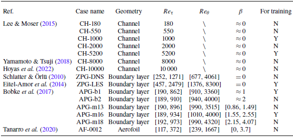
We use data from Schlatter & Örlü (Reference Schlatter and Örlü2010), Eitel-Amor, Örlü & Schlatter (Reference Eitel-Amor, Örlü and Schlatter2014), Lee & Moser (Reference Lee and Moser2015), Bobke et al. (Reference Bobke, Vinuesa, Örlü and Schlatter2017), Yamamoto & Tsuji (Reference Yamamoto and Tsuji2018), Tanarro, Vinuesa & Schlatter (Reference Tanarro, Vinuesa and Schlatter2020), Hoyas et al. (Reference Hoyas, Oberlack, Alcántara-Ávila, Kraheberger and Laux2022) for training and validation. The datasets from Lee & Moser (Reference Lee and Moser2015), Yamamoto & Tsuji (Reference Yamamoto and Tsuji2018) and Hoyas et al. (Reference Hoyas, Oberlack, Alcántara-Ávila, Kraheberger and Laux2022) correspond to plane channel flows. The data from Schlatter & Örlü (Reference Schlatter and Örlü2010) and Eitel-Amor et al. (Reference Eitel-Amor, Örlü and Schlatter2014) pertain to ZPGTBLs, while Bobke et al. (Reference Bobke, Vinuesa, Örlü and Schlatter2017) provide data for PGTBLs. The dataset from Tanarro et al. (Reference Tanarro, Vinuesa and Schlatter2020) corresponds to aerofoil flows. Table 2 provides further details, listing the reference, geometry, range of friction Reynolds number
 $Re_\tau = u_\tau \delta / \nu$
, momentum-thickness-based Reynolds number
 $Re_\theta = U_e \theta / \nu$
(when applicable), the Clauser pressure-gradient parameter
 $\beta = (\delta ^* / \tau _w) \, {\rm d}P/{\rm d}x$
(when applicable), and whether the case is used for training. Here,
 $u_\tau = \sqrt {\tau _w / \rho }$
is the friction velocity,
 $U_e$
is the free-stream velocity,
 $\theta$
is the momentum thickness,
 $\delta ^*$
is the displacement thickness, and
 $\tau _w$
is the wall shear stress.
Details of the data in Lee & Moser (Reference Lee and Moser2015), Yamamoto & Tsuji (Reference Yamamoto and Tsuji2018), Hoyas et al. (Reference Hoyas, Oberlack, Alcántara-Ávila, Kraheberger and Laux2022), Schlatter & Örlü (Reference Schlatter and Örlü2010), Eitel-Amor et al. (Reference Eitel-Amor, Örlü and Schlatter2014), Bobke et al. (Reference Bobke, Vinuesa, Örlü and Schlatter2017) and Tanarro et al. (Reference Tanarro, Vinuesa and Schlatter2020). In the last column, Y and N represent Yes and No.

3. Turbulence closures
3.1. Details of training
We apply SR to learn corrections to the mixing length model to account for various types of flow physics. The machine-learning process involves multiple stages, progressively incorporating increasingly complex flows – though none of the flows used for training is complex in an absolute sense. Again, the key novelty lies in addressing the generalisability issue and enabling transfer learning rather than in complex flows.
We first train on plane channel flow, where the mean flow is one-dimensional and depends only on the wall-normal coordinate
 $y$
. Prior knowledge of the mixing length is incorporated: rather than using the mixing length
 $l$
as the direct target, we train for
 $l/l_{\textit{VD}}$
– a strategy previously adopted in Yang et al. (Reference Yang, Zafar, Wang and Xiao2019), where the target was the mean velocity and the prior knowledge was the law of the wall. This approach has proven effective. Here,
 $l_{\textit{VD}} = \kappa y D$
,
 $D= (1-\exp (-y^+/A^+))$
represents an established model for the mixing length in the inner layer (van Driest Reference van Driest1956), where
 $A^+ = 26$
is the constant. The training dataset includes channel flow cases CH-1000 and CH-5200, with friction Reynolds numbers
 $Re_\tau = 1000$
and
 $5200$
, respectively.
Applying SR to the channel flow data yields
 \begin{equation} l = \kappa y \left [1-\exp \left(-\frac {y^+}{A^+}\right)\right]\left[1 - \exp \bigg(-\frac {\sqrt {y^+}}{3.6}\bigg) + \frac {1.21\big(y^+ + \sqrt {y^+}\big)}{\exp (\sqrt {y^+}) + 8.19}\right]^{-1}\exp \left(-\frac {y}{H}\right). \end{equation}
Due to the white-box nature of SR, we can decompose the learned closure into the prior model
 $l_{\textit{VD}}$
, an inner-layer correction
 $f_{{in}}$
, and an outer-layer correction
 $g_{{out}}$
:
 \begin{equation} l = l_{\textit{VD}}\, f_{ {in}}(y^+)\, g_{ {out}}(y/H), \end{equation}
where
 \begin{equation} f_{ {in}} = \left [1 - \exp \bigg(-\dfrac {\sqrt {y^+}}{3.6}\bigg) + \dfrac {1.21\big(y^+ + \sqrt {y^+}\big)}{\exp (\sqrt {y^+}) + 8.19}\right]^{-1} \end{equation}
and
 \begin{equation} g_{ {out}} = \exp \left (-\dfrac {y}{H}\right). \end{equation}
Here, the Reynolds number information is implicitly included since
 $Re_\tau =y^+/(y/H)$
. Since the inner layer of all wall-bounded flows is universal, the inner-layer correction
 $f_{ {in}}$
is expected to generalise across different flows. Conversely, the outer-layer correction
 $g_{ {out}}$
is specific to plane channel flow. If the obtained model is not decomposed into its generalisable and dataset-specific components, then it would remain applicable only to channel flow – highlighting why prior data-driven models often fail to generalise. By explicitly identifying and retaining only the generalisable components, we enable both generalisation and transfer learning. Equation (3.2) can be obtained through physical arguments. The purpose of this exercise is to show that SR, a machine-learning tool, has the ability to identify the internal structure of a function – a capability that black-box-type function approximators generally lack.
Before progressing to the next flow configuration, several remarks on (3.1) are warranted. First, the form in (3.1) is a result of SR, whereas (3.2) represents our physical interpretation of the white-box model in (3.1). In other words, SR provides a transparent, interpretable model from which (3.2) can be extracted. Once the structure in (3.2) is known, one can indeed use any regression method – such as neural networks – to learn
 $f_{ {in}}$
and
 $g_{ {out}}$
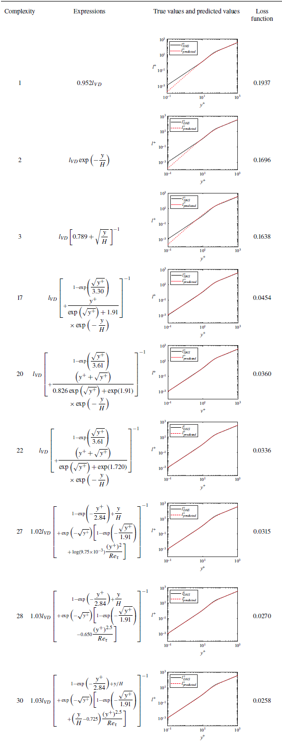
. The expression in (3.1) is a result of combined considerations of complexity and accuracy. Second, like any other machine learning, SR is also susceptible to overfitting. Table 3 shows the complexity level, the corresponding expression and the loss function. Figure 4 illustrates the complexity–accuracy trade-off. We observed that beyond complexity level 20, further increases in complexity yield only marginal improvements in the loss function. This poor complexity–accuracy trade-off indicates overfitting – although overfitting is formally defined as a lack of generalisation to unseen data, in SR literature, poor complexity–accuracy trade-off is often used as an indicator of overfitting. The above is why we picked the expression at complexity level 20 ((3.1) corresponds to the expression at complexity level 20). Admittedly, the threshold at which additional complexity yields negligible reduction in the loss function is somewhat subjective. Nonetheless, the form in (3.2) is robust. We could have selected the expressions at complexity levels 17–22, all of which conform to (3.2). For completeness, we also showcase expressions at a few complexity levels from 1 to 30. We see that too low a complexity level leads to clear underfitting, and too high a complexity level leads to overfitting, i.e. an overly complex expression with practically the same loss function.
The expressions at different complexities, and their predicted values and loss. The expressions at complexities 1, 2, 3 correspond to underfitting. The expressions at complexities 17, 20, 22 are well-generalised, while the expressions at complexities 27, 28, 30 correspond to overfitting.

Third, the redundant input
 $Re_\tau$
does not show up in the expression, showing that it is indeed redundant and that the training is robust to redundant inputs. Fourth, SR yields the correct asymptotic behaviour for the eddy viscosity at the wall. The eddy viscosity should scale as
 $\nu _t \sim O(y^3)$
near the wall (Pope Reference Pope2001) because
 \begin{align} \nonumber\\[-18pt]\lim _{y\to 0}\nu _t=\lim _{y\to 0}\dfrac {-\left \langle u^{\prime}v^{\prime}\right \rangle }{{{\rm d}U}/{{\rm d}y}}\sim \lim _{y\to 0}\dfrac {y^3}{1} \sim y^3; \end{align}
however, the conventional model in van Driest (Reference van Driest1956) behaves as
 \begin{equation} \lim _{y\to 0}\nu _t = \lim _{y\to 0} l^2 \dfrac {{\rm d}U}{{\rm d}y} \sim O(y^4), \end{equation}
which is inaccurate. The closure in (3.1), on the other hand, gives
 \begin{equation} \lim _{y\to 0}\nu _t = \lim _{y\to 0} (l_{\textit{VD}}\, f_{ {in}}\, g_{ {out}})^2 \dfrac {{\rm d}U}{{\rm d}y} \sim O(y^3), \end{equation}
which correctly recovers the expected asymptotic behaviour. This is also evident from figure 6(a), where we compare the SR model, the conventional van Driest model, and DNS data for
 $Re_{\tau }$
ranging from 180 to 10 000. The goal here is to validate the SR methodology by showing that the obtained expressions closely match the data. Comparison to existing turbulence models will be introduced in § 4, where we show results for a posteriori tests. Fifth, we trained the SR model to predict the ratio
 $l/l_{\textit{VD}}$
. This formulation isolates the correction relative to the baseline model. We may train the SR model to directly predict
 $l$
. The resulting expression still takes the form of (3.2), and the inner layer correction
 $f_{ {in, 2}}$
equals
 $f_{ {in}}D$
in terms of the performance, as shown in figure 5. However, unless we rearrange
 $f_{ {in, 2}}$
, the van Driest function does not emerge explicitly.
Normalised loss as a function of complexity from (a) one realisation corresponding to table 3, and (b) another realisation. The losses are normalised by the loss at complexity level 1. Filled symbols indicate that the expressions conform to the structure in (3.2). The two black solid lines represent finite and diminishing returns in loss reduction when increasing complexity before and beyond level 20. The skipping (e.g. 18, 21, 29 in (a)) is due to the fact that PySR will not return an expression with a loss function higher than that of the expression of a lower complexity.

A comparison between
 $f_{{in}}D$
and
 $f_{{in},2}$
, which is
 $\big[1+ 562.4\big[48.5\sqrt {y^+}+\sqrt {y^+}\exp \big(\sqrt {y^+}\big)\big]^{-1}\big]^{-1}$
.

We also distinguish between analysis and interpretation. Analysis involves examining the behaviour of a model and can be applied to both black-box models, such as neural networks, and white-box models, such as SR-derived expressions. Physical interpretation, on the other hand, involves parsing a model and assigning clear physical meanings to its components, which is typically possible only for white-box models. For example, (3.7) represents an analysis of the SR model, whereas (3.2) demonstrates its physical interpretation. While analysis may provide insights, it does not inherently lead to generalisability. In contrast, by distinguishing between generalisable and dataset-specific components, physical interpretation provides a path to achieving generalisability. This study focuses on physical interpretation. For the result in (3.1), our interpretation is the parsing of the equation into an inner-layer correction
 $f_{{in}}$
and an outer-layer correction
 $g_{{out}}$
. We can further interpret the two corrections as follows. First,
 $f_{{in}}$
modifies the mixing length in the inner layer, compensating for the overly rapid decay of eddy viscosity in the viscous sublayer. This behaviour is evident from (3.5), (3.6), (3.7) and figure 6(a). In contrast,
 $g_{{out}}$
adjusts the outer-layer mixing length by accounting for a slower-than-linear growth with distance from the wall.
(a) Eddy viscosity in channel. (b) Eddy viscosity in ZPG-LES. (c) Eddy viscosity in APG-b1. The symbols are reference DNS data. The van Driest model corresponds to the black dashed line.

Next, we train the model on the ZPGTBL. This flow is slightly more complex than in the plane channel. The mean flow is a function of the streamwise coordinate
 $ x$
and the wall-normal coordinate
 $ y$
. If we were to follow the conventional approach, then the model trained using channel flow data would yield poor results for the boundary layer, requiring training from scratch. However, because we parse the white-box model in (3.1) into a generalisable inner-layer part and a data-specific outer-layer part, here, we can take the generalisable part and use it for our training for boundary-layer flows. Specifically, we build on the generalisable inner-layer correction, and only train for an outer-layer correction for the boundary-layer configuration. Data for case ZPG-LES at a few Reynolds numbers between
 $Re_\theta =1376$
and
 $Re_\theta =8183$
are used for training. The resulting outer-layer correction takes the form
 \begin{equation} h_{ {out}}=\tanh \left [\left (0.215 + (Re_\tau + 1.0086^{Re_\tau })^{-0.62}\right)\left (\dfrac {y}{\delta _{99}}\right)^{-1}\right], \end{equation}
where
 $h_{{out}}$
plays a similar role to
 $g_{{out}}$
, but employs a functional form based on
 $\tanh (a(\delta _{99}/y))$
to achieve the slower-than-linear growth. The Reynolds-number-dependent prefactor
 $a$
captures finite Reynolds number effects (Klewicki Reference Klewicki2010), and asymptotically approaches 0.215 at high Reynolds numbers. Note that while
 $Re_\tau$
is a redundant input when we train against channel flow data, it is not a redundant input here and cannot be obtained from the other input,
 $y/\delta _{99}$
. When (3.8) is used, the function
 $h_{out}$
will replace
 $g_{out}$
in (3.4). Here, we have assumed a multiplicative correction rather than, for example, an additive correction. This choice should not affect the model’s performance, as the two are mathematically equivalent. For a baseline model denoted as
 $B$
, a multiplicative correction
 $1 + C_m$
and an additive correction
 $C_a$
satisfy the relationship
 $B C_m = C_a$
. The resulting eddy viscosity is compared against the high-fidelity LES data (
 $Re_\theta$
from 1376 to 8183) in figure 6(b), showing a close agreement between the two. The van Driest model is also shown for comparison purposes. We note that the van Driest model alone does not constitute a viable turbulence model as the linear behaviour in the outer layer must be damped using e.g. the outer-layer correction in Baldwin & Lomax (Reference Baldwin and Lomax1978). We see that the van Driest model generally overpredicts the eddy viscosity.
Finally, we consider pressure gradient. In external aerodynamics applications, pressure gradients arise due to surface curvatures (Gungor et al. Reference Gungor, Maciel, Simens and Soria2016), often leading to flow separation, which remains challenging to model. With a few exceptions (Chen et al. Reference Chen, Bin, Yang, Shi, Abkar and Park2023b
; Yang et al. Reference Yang, Chen, Zhang and Kunz2024b
), previous PGTBL modelling efforts have relied heavily on heuristics and empirical methods (Nickels Reference Nickels2004; Romero et al. Reference Romero, Zimmerman, Philip, White and Klewicki2022). Machine learning has also been applied to pressure-gradient-dominated flows, such as periodic hills, backward-facing steps and separated flows (Yan, Zhang & Chen Reference Yan, Zhang and Chen2022; Shan et al. Reference Shan, Liu, Cao, Sun and Zhang2023, Reference Shan, Sun, Cao, Zhang and Xia2024; Tang et al. Reference Tang, Wang, Wang and Tian2023; Wang & Zhang Reference Wang and Zhang2023; Zhou et al. Reference Zhou, Whitmore, Griffin and Bae2023; Arranz et al. Reference Arranz, Ling, Costa, Goc and Lozano-Durán2024; Zhou & Bae Reference Zhou and Bae2024). However, this study represents the first instance of isolating a machine-learned correction specifically for pressure-gradient effects. Here, we train the model on PGTBLs at conditions corresponding to cases APG-b1 and APG-m16. The training data cover a Reynolds number range from
 $Re_\theta = 940$
to
 $Re_\theta = 4000$
, and a Clauser pressure-gradient parameter range between 1 and 2.55. Building on the previously obtained inner-layer correction
 $f_{ {in}}$
and the outer-layer correction
 $h_{ {out}}$
for TBLs, we learn an additional correction for the pressure gradient. Symbolic regression yields the following pressure-gradient correction:
 \begin{equation} \gamma _{ {PG}} = 1 + 18 \left(\dfrac{{\rm d}P}{{\rm d}x}\right)^+\left [1-\tanh \left (\dfrac {y^+-12.7}{14}\right)\right]. \end{equation}
When used in RANS, the correction factor is incorporated into the mixing length as a multiplicative correction:
 \begin{equation} l = l_{\textit{VD}}\, f_{ {in}}\, h_{ {out}}\, \gamma _{ {PG}}. \end{equation}
Here,
 $\gamma _{ {PG}}$
modulates the eddy viscosity in the presence of streamwise pressure gradients: it reduces the eddy viscosity in favourable PGTBLs, and increases it in adverse pressure-gradient cases through the
 $b({\rm d}P/{\rm d}x)$
term. The prefactor
 $b$
, which varies with
 $y^+$
, ensures that the influence of the pressure gradient diminishes near the wall. According to this result, pressure gradients do not significantly affect the validity of the mixing length formulation in the outer region. This finding aligns with the classic work by Kays et al. (Reference Kays, Crawford and Weigand1980), who noted that for PGTBLs, modifications to the mixing length model are primarily needed in the viscous layer. The fact that the present SR approach correctly identifies this adjustment highlights the strength of our methodology. The resulting eddy viscosity is compared against the data for case APG-b1 in figure 6(c), showing close agreement between the two, while the van Driest model performs poorly.
In summary, we apply SR and train our model on plane channel flow, ZPGTBLs and PGTBLs. The inner-layer correction obtained from plane channel flow is generalisable and is retained in all subsequent training. The two outer-layer corrections,
 $ g_{ {out}}$
and
 $ h_{ {out}}$
, are specific to channel flow and TBLs, respectively, with the boundary-layer correction being retained during training on PGTBLs. Finally, a pressure-gradient correction is learned through training on PGTBLs. Again, the novelty of the present approach lies in the identification of generalisable components within machine-learned models, and the systematic utilisation of these components in subsequent training, thereby overcoming the generalisability issue.
4. Verification and validation
We have assigned clear physical interpretations to the models obtained in § 3. The purpose of this section is to evaluate their generalisability. The test cases are chosen carefully. They are simple enough to ensure clarity in the machine-learning methodology without ambiguity in flow physics, yet challenging enough that existing RANS closures struggle – allowing us to demonstrate the advantages of our approach. Furthermore, these tests will illustrate that the failure to distinguish between generalisable and data-specific flow physics is the fundamental reason why machine-learned models often lack generalisability. Throughout this section, we will include results of the SA and SST models for comparison purposes. All flow variables, including those used as inputs in SR models, are computed dynamically as we solve the RANS equations.
4.1. Seen geometries
We first consider plane channel flow. The SR model in this case contains the inner-layer correction
 $f_{ {in}}$
and the channel-specific outer-layer correction
 $g_{ {out}}$
. The RANS details are provided in § 2. Further details of the computational set-up for plane channel flow can be found on the TMR site and are not repeated here for brevity. Figure 7 presents the results, with Reynolds numbers ranging from
 $Re_\tau = 180$
to
 $Re_\tau = 10\,000$
. While the SR model has been trained on the channel configuration, it has not seen all Reynolds numbers. Figure 7(a, b) show the mean velocity profiles and the corresponding Reynolds stresses, demonstrating close agreement between the present SR model and the DNS data across all Reynolds numbers. This result confirms that
 $f_{ {in}}$
and
 $g_{ {out}}$
generalise well to both seen and unseen Reynolds numbers.
Channel flow results. The SR model contains the inner-layer correction
 $f_{ {in}}$
and the channel-specific outer-layer correction
 $g_{ {out}}$
. The present SR model has seen the configuration but not all the Reynolds numbers. (a) Mean velocity profile. For illustration purposes, neighbouring profiles are displaced by
 $10$
plus units in the vertical axis. (b) Reynolds shear stress. The symbols are DNS reference data.

The ZPGTBL results. The present SR model has seen the configuration but not all the Reynolds numbers. (a) The skin friction coefficient: SR-TBL denotes the mixing length model with the inner-layer correction
 $f_{ {in}}$
and the TBL-specific outer-layer correction
 $h_{ {out}}$
; SR-CH denotes the mixing length model with the inner-layer correction
 $f_{ {in}}$
and the channel-specific outer-layer correction
 $g_{ {out}}$
. Both LES and DNS are of higher fidelity than RANS, and are reference data. (b, d) Mean velocity profile for
 $Re_\theta \approx 670$
and 8200. (c, e) Reynolds shear stress for
 $Re_\theta \approx 670$
and 8200.

Next, we consider ZPGTBLs. As before, we replicate the set-up from the TMR website. Figure 8(a) presents the skin friction coefficient as a function of
 $Re_\theta$
. We compare high-fidelity data, the SA and SST models, the model with the inner-layer correction
 $f_{ {in}}$
and the TBL-specific outer-layer correction
 $h_{ {out}}$
, and the model with
 $f_{ {in}}$
along with the channel-specific outer-layer correction
 $g_{ {out}}$
. The SST and SA models predict the friction coefficient at high Reynolds number, although there are errors in the low-Reynolds-number regime. While the model containing
 $f_{ {in}}$
and
 $h_{ {out}}$
closely matches the high-fidelity data, applying the channel-specific outer-layer correction
 $g_{ {out}}$
to the boundary-layer configuration results in significant errors. This confirms that failing to distinguish between generalisable and dataset-specific flow physics is the reason why existing machine-learning models struggle to generalise beyond their training datasets. In figure 8(b–e), we compare the model incorporating
 $f_{ {in}}$
and
 $h_{ {out}}$
with the SA and SST models for their predictions of the mean flow and Reynolds shear stress. Figure 8(b, d) show the mean velocity profiles at
 $Re_\theta \approx 670$
, which is below the training Reynolds number, and
 $Re_\theta \approx 8200$
, which is above the training Reynolds number, while figure 8(c, e) show the corresponding Reynolds stresses. The results indicate that the present SR model provides more accurate predictions of the mean flow and Reynolds shear stress compared to the SA and SST models. The SA and SST models do not capture the mean flow at low Reynolds numbers as shown in figure 8(b). These findings demonstrate the following: (i) the inner-layer correction
 $f_{ {in}}$
generalises well across different types of wall-bounded flows; (ii) the outer-layer correction
 $g_{ {out}}$
is specific to channel flow and degrades performance when applied to boundary-layer flows; (iii) the outer-layer correction
 $h_{ {out}}$
generalises across different Reynolds numbers.
The PGTBL results. The present SR model has seen the configuration but not all the pressure-gradient conditions. (a) The skin friction coefficient: SR-PG denotes the SR model that contains the inner-layer correction
 $f_{ {in}}$
, the boundary-layer-specific outer-layer correction
 $h_{ {out}}$
and the PG-specific correction
 $\gamma _{ {PG}}$
; SR-TBL denotes the SR model that contains the inner-layer correction
 $f_{ {in}}$
and the boundary-layer-specific outer-layer correction
 $h_{ {out}}$
. (b, d, f) Velocity profiles at
 $x/L = 1000, 1500, 2000$
. (c, e, g) Reynolds shear stress at
 $x/L = 1000, 1500, 2000$
.

The NACA0012 results. The SR model contains the inner layer correction
 $f_{ {in}}$
, the boundary-layer specfic outer-layer correction
 $h_{ {out}}$
, and the pressure-gradient correction
 $\gamma _{ {PG}}$
: (a) pressure coefficient
 $-C_p$
; (b) skin friction coefficient
 $C_f$
. In the LES, the boundary layer was tripped at 10 % of the chord length from the leading edge on sides of the wing section. As a result, LES data before this location are not available. (c, e, g) Velocity profiles at
 $x/c = 0.3, 0.6, 0.9$
. (d, f, h) Reynolds shear stress at
 $x/c = 0.3, 0.6, 0.9$
.

A priori test of the SR model for LES wall modelling. Here, the SR model contains the inner layer correction
 $f_{ {in}}$
and the pressure-gradient correction
 $\gamma _{ {PG}}$
: (a) APG-b1, (b) APG-b2, (c) APG-m13, (d) APG-m16, (e) APG-m18.

Finaly, we consider PGTBLs. The flow condition corresponds to case APG-m18. The computational grid matches that of the DNS, with the first off-wall grid point located within
 $y^+ \leqslant 1$
. The pressure-gradient condition in this case exceeds that of the training data; see table 2. The pressure-gradient correction
 $\gamma _{PG}$
is incorporated into the mixing length model as a multiplicative correction. Figure 9 presents the results. Figure 9(a) shows the skin friction coefficient as a function of
 $Re_\theta$
. We compare the high-fidelity data, the SA and SST models, the model incorporating the inner-layer correction
 $f_{ {in}}$
, the outer-layer correction
 $h_{ {out}}$
and the pressure-gradient correction
 $\gamma _{ {PG}}$
, and the model with only the inner-layer correction
 $f_{ {in}}$
and outer-layer correction
 $h_{ {out}}$
. The results demonstrate that incorporating the pressure-gradient correction significantly improves the prediction of the skin friction coefficient. Figure 9(b–g) present the mean velocity profiles and Reynolds shear stress results at conditions both within and outside the training dataset. We see that the inclusion of the pressure-gradient correction improves velocity and Reynolds shear stress predictions as well. Errors in the Reynolds stresses are observed in all models, particularly at larger
 $x/L$
. This is attributed to the limitation of eddy-viscosity models to capture history effects: modelling errors at upstream locations accumulate as the flow progresses downstream (Yang et al. Reference Yang, Chen, Zhang and Kunz2024b
). In all, these PGTBL results demonstrate: (i) the outer-layer correction
 $h_{out}$
generalises to PGTBLs; (ii) the pressure-gradient correction
 $\gamma _{PG}$
generalises across pressure gradient beyond the training dataset.
4.2. Unseen geometry
We validate the SR models on an unseen configuration, specifically the NACA0012 aerofoil. This case involves both boundary-layer physics and pressure-gradient effects. The set-up follows that on the TMR site (Rumsey Reference Rumsey2019). As before, the first-layer cell height is below
 $y^+ \lt 1$
, and the grid is sublayer resolved. The aerofoil is at angle of attack
 $0^\circ$
, with Reynolds number
 $Re_c = 4\,00\,000$
. The flow experiences a favourable pressure gradient near the leading edge, and an adverse pressure gradient near the trailing edge, making it a strong test case for evaluating the pressure-gradient correction
 $\gamma _{ {PG}}$
. Figure 10 presents the results. Figure 10(a, b) show the negative pressure coefficient
 $-C_p = 2(P_\infty -P)/(\rho U_\infty ^2)$
and skin friction coefficient
 $C_f$
, while figure 10(c, e, g) depict velocity profiles as functions of
 $y^+$
at
 $x/c = 0.3, 0.6, 0.9$
. The corresponding Reynolds stresses are shown in figure 10(d, f, h). For comparison, results from the SST and SA models are also included. Several observations emerge. The conventional RANS models underpredict the skin friction coefficient and overpredict velocity. Additionally, their Reynolds shear stress predictions deviate significantly from the reference data. In contrast, the present SR model closely matches the high-fidelity reference data, with only minor errors in Reynolds shear stress. These results validate both the effectiveness and generalisability of the symbolic models.
4.3. Near-wall turbulence modelling for LES
The discussion so far has been limited to the relatively simplistic mixing length model in the context of RANS modelling. While this may seem restrictive, as modern RANS models rely primarily on transport equations rather than local algebraic closures, the mixing length model remains the dominant approach for near-wall modelling in LES (Bose & Park Reference Bose and Park2018). In this subsection, we explore the directly applicability of our SR models for LES wall modelling. For simplicity, we follow Chen et al. (Reference Chen, Lv, Xu, Shi and Yang2022a
) and conduct an a priori study. Specifically, the wall model equation is solved from the wall, i.e.
 $y/\delta = 0$
up to the wall model/LES matching location. We then compare the wall model results to those from wall-resolved LES (WRLES). We consider PGTBLs, specifically the five cases detailed in Bobke et al. (Reference Bobke, Vinuesa, Örlü and Schlatter2017). The wall shear stress is computed using information at
 $y=0.15\delta, 0.30\delta$
, typical wall-model/LES matching locations. We compare the mixing length model incorporating the
 $f_{ {in}}$
and
 $\gamma _{ {PG}}$
corrections with the conventional mixing length model in Piomelli (Reference Piomelli2008), which constutites the equilibrium wall model (EWM). The results are presented in figure 11. The SR model proves to be highly effective and robust, significantly improving wall shear stress predictions across all pressure-gradient conditions in PGTBLs, and yielding essentially the same results for the two matching locations. The EWM, on the other hand, is less accurate, and shows notable dependence on the matching location. Although the primary focus of this paper is on methodology and addressing the generalisability issue rather than developing new models, these results demonstrate the direct utility of the resulting models in Wall-modeled Large-Eddy Simulations.
5. Conclusions
Machine-learned turbulence models often struggle to generalise beyond their training datasets. Given the inherent complexity of turbulence, reliance on large datasets alone is not a practical solution. Previous efforts to enhance generalisability have focused on preserving symmetries, such as Galilean invariance, but these approaches have achieved only limited success, and the root cause of the lack of generalisability remains unclear.
This paper addresses the generalisability challenge. We first identify its root cause: the failure to distinguish between flow physics that generalise across configurations and those specific to training data. To resolve this issue, we decompose expressions obtained through symbolic regression (SR) into components that are universally applicable and those tied to the training dataset. When applying the model to flows beyond the training set – whether in the context of RANS or model retraining – only the generalisable components are retained. The SR is critical in the initial discovery process because it yields white-box models that are amenable to physical interpretation. A black-box model, on the other hand, would obscure the underlying structure and make it difficult to isolate generalisable versus data-specific physics.
Using this approach, we trained models on channel flow, ZPGTBLs and PGTBLs. This yielded generalisable corrections to the conventional mixing length model, including inner-layer and pressure-gradient corrections, as well as outer-layer adjustments specific to channel and boundary-layer flows. By applying these machine-learned mixing length closures, we achieved superior results in both familiar configurations (channel and boundary-layer flows) and an unfamiliar case (aerofoil flow), demonstrating the robustness and generalisability of the proposed corrections. These results demonstrates that data-driven models can have generalisability similar to that of conventional models.
While this study focuses on the methodology rather than the resulting model, the utility of the SR models is still demonstrated in the context of LES wall modelling. Extending our methodology to transport-type models is also possible. The process follows the same three steps outlined in this paper: first, identifying relevant features such as
 $y^+$
,
 $y/\delta$
,
 $r$
,
 $P/D$
and
 $\chi$
(Srivastava et al. Reference Srivastava, Rumsey, Coleman and Wang2024); second, applying SR to learn new terms for the transport equation; and third, parsing the learned terms into components that represent generalisable and training-specific flow physics, retaining only the former.
We believe that the results presented here pave the way for developing truly predictive machine-learned turbulence models capable of addressing complex turbulence challenges.
Funding
Z.Y., X.S. and W.Z. acknowledge financial support from the National Natural Science Foundation of China (no. 92152301, no. U2441211, no. U23B6009), the National Key Research and Development Programme of China (no. 2022YFB4300200) and Shaanxi Innovative Research Team of Artificial Intelligence for Fluid Mechanics (no. 2024RS-CXTD-16).
Declaration of interests
The authors report no conflict of interest.
Appendix A. Symbolic regression algorithm
Symbolic regression is a machine-learning technique that searches for analytical expressions that best fit a given dataset. Unlike traditional regression, which assumes a predefined functional form (e.g. linear or polynomial), SR explores a vast space of mathematical expressions constructed from a predefined set of operators (e.g. addition, multiplication, exponentiation). In this work, we use the PySR library, which implements a variant of genetic programming optimised for SR. The core idea is to evolve a population of candidate expressions over multiple generations, progressively improving their accuracy and simplicity. The process begins with an initial population of randomly generated expressions. Each expression is evaluated using a fitness score, typically the mean squared error with respect to the training data. The top-performing expressions are retained and used to generate a new population through two key mechanisms: crossover that combines parts of two parent expressions to produce new candidate expressions, and mutation that randomly modifies parts of an expression to introduce diversity. Throughout the iterations, PySR maintains a ‘hall of fame’ set that stores the best-performing expressions across all populations and generations, ensuring that promising candidates are preserved.
We summarise the SR algorithm as used in this work in Algorithm 1. Our implementation uses 64 independent populations (‘islands’), each containing 500 expressions. The algorithm runs for 300 iterations, and includes mechanisms for migration and parallel evolution across populations.
Overview of the symbolic regression procedure using PySR

Appendix B. Repeatability of (3.2)
To assess the repeatability of (3.2), we trained the SR algorithm on three distinct groups of data. Under the settings summarised in table 1, SR consistently rediscovered the structure of the mixing length expression in (3.2), as indicated by the fraction in table 4. Because both
 $f_{{in}}$
and
 $g_{{out}}$
are functions of a single variable, we can visualise and compare them across different runs. As shown in figure 12(a, b), the resulting expressions yield nearly identical profiles, confirming the robustness of the SR procedure under the specified configuration. Furthermore, we applied the discovered mixing length model to the CH-10 000 case. The predicted results exhibit excellent agreement across different SR runs, as shown in figure 12(c, d), further demonstrating the repeatability and generalisability of the obtained expression.
The training data contained in each group. The fraction given is the number of times that (3.2) is rediscovered divided by the number of total trials. The expression does not conform to (3.2) every time because CH-180 is at too low a Reynolds number and there are still low Reynolds number effects.

The results of repeated experiments: (a)
 $f_{ {in}}$
discovered across different runs; (b)
 $g_{ {out}}$
discovered across different runs; (c) predicted velocity profiles; (d) predicted Reynolds shear stress.