2. DICKEY ET AL. AND HYLLEBERG ET AL. SEASONAL UNIT ROOT TESTS

Consider the seasonal time series process, {x_t}, observed with constant periodicity S, S > 1, generated according to

where α(z) is an autoregressive (AR) polynomial of order

, and L is the usual lag operator, L^kx_t = x_t−k, k = 0,1,…. The roots of α(z) = 0 either lie (distinctly) on the unit circle, |z| = 1, at some or all of the zero and seasonal spectral frequencies, exp(±i2πk/S), k = 0,…,[S/2], [·] denoting the integer part of its argument, or lie outside the unit circle. Following Tanaka (1996, pp. 355–361), we consider the following three cases, indexed by ξ, for the deterministic kernel μ_t: (i) ξ = 0, μ_t = 0; (ii)

and (iii)

, where D_s,t = 1 if t lies in season s, s = 1,…,S, zero otherwise. To yield asymptotically pivotal statistics, the (observed) initial values are assumed to satisfy T^−1/2x_−j →^p 0, j = 0,…,S − 1, under case (i). This assumption may otherwise be dropped.

2.1. Dickey et al. Tests

Dickey et al. specialize (2.1) to the case of the pure seasonal AR(1); i.e., α(z) ≡ (1 − ρ_S z^S). In this case, one may rewrite (2.1) as

t = 1,…,T, where μ_t* ≡ α(L)μ_t. In the context of (2.2), Dickey et al. consider testing the null hypothesis

against the one-sided stationary alternative

Under H₀ of (2.3), the roots of the characteristic equation 1 − z^S = 0 are exp(±i2πk/S), k = 0,…,[S/2] . Consequently, {x_t} admits unit roots at both the zero, ω₀ ≡ 0, and seasonal spectral frequencies ω_k ≡ 2πk/S, k = 0,…,[S/2] , so that the seasonally differenced process Δ_S x_t, where Δ_S ≡ (1 − L^S), is stable and invertible. In contrast, under H₁ of (2.4), the roots of 1 − ρ_S z^S = 0 remain of equal moduli but all lie outside the unit circle.

To test H₀ of (2.3) against H₁ of (2.4), under the assumption that α(z) ≡ (1 − ρ_S z^S) in (2.1), Dickey et al. suggest the normalized coefficient estimate

, obtained from ordinary least squares (OLS) estimation of (2.2), i.e.,

and the corresponding studentized statistic

where x_t⁰ ≡ x_t and where x_t¹ and x_t² are the OLS residuals from the regression of x_t on seasonal intercepts and on seasonal intercepts and seasonal trends, respectively, and

.

Under H₀ of (2.3), it is readily demonstrated that the limiting distribution of the Dickey et al. test statistics

of (2.5) and t_ρS=1 of (2.6) are as follows:

where ⇒ denotes weak convergence and the W_s^ξ(r), s = 1,…,S, are a set of S independent standard, demeaned, and demeaned and detrended Brownian motion processes for ξ = 0, ξ = 1, and ξ = 2, respectively. Critical values from the distributions in (2.7) and (2.8) are provided in Dickey et al. for ξ = 0 and ξ = 1, whereas Tanaka (1996, pp. 262–264) provides critical values for η_ξ(S)/S for ξ = 0,1, and 2 in Tables 7.4, 7.5, and 7.7, respectively. Critical values for τ_ξ(S), ξ = 0,1,2 may also be calculated using a Gram–Charlier approximation (see Nabeya, 2000, 2001). Moreover, under H₁, it is readily seen that

and t_ρS=1 are consistent tests, both diverging to minus infinity.

2.2. Hylleberg et al. Tests

Consider (2.1) again. Following Smith and Taylor (1999, equation (4.17), p. 9) and Hylleberg et al., linearizing α(z) in (2.1) around the zero and seasonal frequency unit roots, exp(±i2πk/S), k = 0,…,[S/2] , yields the auxiliary regression equation

t = 1,…,T, omitting the term π_S/2 x_S/2,t−1 if S is odd. In contrast to (2.2), (2.9) is an unrestricted exact linear reparameterization of (2.1). In the context of (2.9), corresponding to the zero and seasonal frequencies ω_k = 2πk/S, k = 0,…,[S/2] ,

k = 1,…,S*, where S* = (S/2) − 1 (if S is even) and [S/2] (if S is odd).

The seasonal unit root null hypothesis H₀ of (2.3) implies π_j = 0, j = 0,…, S − 1, in (2.9). Consequently, the regression F-test, F_0…[S/2], for the exclusion of the regressors {x_j,t−1}_j=0^S−1 from (2.9) provides a test of H₀. However, unlike the Dickey et al. statistics the alternative hypothesis is now of stationarity at least one (i.e., not necessarily all) of the zero and seasonal frequencies. Moreover, as demonstrated in Hylleberg et al. (1990) and Smith and Taylor (1999), H₀ is the intersection of the subsidiary null hypotheses: H_0,0 : π₀ = 0, a unit root at ω₀; H_0,S/2 : π_S/2 = 0, a unit root at ω_S/2 ≡ π (S even); and H_0,k : π_k = π_S−k = 0, a pair of complex conjugate roots at the kth seasonal harmonic frequency ω_k ≡ (2πk/S), k = 1,…,S*. One may therefore consider the following individual frequency unit root statistics from (2.9): t₀ (left-sided) for the exclusion of x_0,t−1; t_S/2 (left-sided) for the exclusion of x_S/2,t−1 (S even); F_k for the exclusion of both x_k,t−1 and x_S−k,t−1, k = 1,…,S*. Limiting null distributions of the preceding statistics from (2.9) are provided in Smith and Taylor (1999), whereas the consistency of the tests under their respective alternatives is demonstrated in Rodrigues (2001) and Taylor (2002a).

As we have seen, the Dickey et al. tests impose the maintained hypothesis that α(z) of (2.1) is a seasonal AR(1) polynomial. This restriction is not imposed by the Hylleberg et al. procedure. If this restriction holds, then (2.2) will be parsimoniously parameterized vis-à-vis (2.9), and one would therefore expect the Dickey et al. statistics to enjoy a finite sample power advantage over the Hylleberg et al. statistics. This is confirmed by the simulation experiments for S = 12 reported in Rodrigues and Osborn (1999), in which the authors argue on the basis of their results that the Dickey et al. tests are generally preferable to the Hylleberg et al. statistics. However, as we show in this paper, if the restriction is violated one may pay an unacceptably high price. As a leading counterexample, the random walk process x_t = x_t−1 + ε_t, where α(z) = 1 − z, is excluded by the restriction. In the next section we focus on the behavior of the Dickey et al. statistics when applied to a random walk process and show that they do not diverge as the sample size increases.

3. ASYMPTOTIC PROPERTIES OF THE DICKEY ET AL. TESTS AGAINST A RANDOM WALK PROCESS

Suppose that the process {x_t} is generated according to the simple random walk, namely,

t = 1,…,T. It is therefore clear that when x_t is generated by (3.1), the Dickey et al. test regression (2.2) is misspecified. In contrast, the Hylleberg et al. test regression remains well specified.

As we now demonstrate in Theorem 3.1, the effects of this misspecification are pronounced; the Dickey et al. statistics

and t_ρS=1 obtained from the OLS estimation of (2.2) will not diverge as the sample size increases.

THEOREM 3.1. If the process {x_t} is generated according to (3.1), then the Dickey et al. statistics

of (2.5) and t_ρS=1 of (2.6) have the following large sample distributions:

where W^ξ(r) is a standard, demeaned, and demeaned and detrended Brownian motion for ξ = 0, ξ = 1 and ξ = 2, respectively.

Remark 3.1. An immediate consequence of (3.2) is that

being O_p(T⁻¹). This holds, regardless of the value of ξ, and tells us immediately that application of the Dickey et al. seasonal unit root test

to a series that is a purely nonseasonal random walk will not deliver a statistic that diverges to minus infinity. The t_ρS=1 statistic also has a nondegenerate limit distribution in this case, and so the same conclusion applies. With nonzero probability, the Dickey et al. tests—taken in isolation from other statistical tests—would then suggest taking seasonal differences, even though the seasonally differenced process {Δ_S x_t} would be strictly noninvertible at each of the seasonal frequencies, ω_k, k = 1,…,S − 1. In contrast, the results in Rodrigues (2001) and Taylor (2002a) show that, under the conditions of Theorem 3.1, the Hylleberg et al. statistic F_0…[S/2] from (2.9) diverges to plus infinity. Indeed, only the t₀ statistic from (2.9), which tests solely for a unit root at the zero frequency, will not diverge in this case, because π₀ = 0.

Remark 3.2. Although we have restricted the error process {ε_t} to be IID(0,σ²), relaxing this by requiring {ε_t} to satisfy only the strong mixing conditions of, among others, Phillips and Perron (1988) merely introduces nuisance parameters into the representations for the limiting null distributions of

and t_ρS=1 (for further details, see the accompanying working paper, Taylor, 2002b). Most important, Remark 3.1 remains valid under such conditions.

Remark 3.3. For a given value of ξ, η_ξ*(S) of (3.2) is equal in distribution to

, a Dickey–Fuller (DF) coefficient distribution (a standard DF distribution for ξ = 0, a demeaned DF distribution for ξ = 1, and a demeaned and detrended DF distribution for ξ = 2), multiplied by the factor S, whereas τ_ξ*(S) of (3.3) is equal in distribution to

, the corresponding DF t-distribution, multiplied by the factor

. Therefore, the greater is S, the more left-shifted will be the lower tails of the distributions of both η_ξ*(S) and τ_ξ*(S).

As Remark 3.3 demonstrates, for a given level α asymptotic critical value, c_α, from the distributions of η_ξ(S) and τ_ξ(S), one may establish the true asymptotic size of the Dickey et al. statistics

and t_ρS=1 when applied to data generated by (3.1). This follows on noting that

. Similarly,

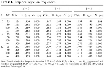
. Table 1 reports these quantities, in the rows labeled ∞, for S = 2, 4, and 12, ξ = 0, 1, and 2, and α = .05.

and t_ρS=1 statistics when applied to data generated by (3.1) over 25, 50, and 100 years of data, i.e., T/S = 25, 50, and 100. The finite sample power of the F_0…[S/2] statistic is also reported. The asymptotic power of the F_0…[S/2] statistic is, of course, unity throughout.

Empirical rejection frequencies

The asymptotic sizes reported in Table 1 were obtained via direct simulation of the

limiting functionals using a sample size of 10,000.

and t_ρS=1 statistics generated by Monte Carlo simulation of data generated according to the seasonal random walk Δ_S x_t = ε_t ∼ IN(0,1), x₀ = ··· = x_1−S = 0, for the given values of T, S, and ξ. Finite sample critical values for the Hylleberg et al. F_0…[S/2] statistic were generated in the same manner. All simulations were programmed using the RNDN random number generator of GAUSS 3.2 on a Pentium II microcomputer and 100,000 replications.

The results reported in Table 1 highlight a number of key points. First, for given T, S, and ξ the observed patterns of size distortion differ little between the

and t_ρS=1 statistics. Even in the limit, we see that the true asymptotic sizes of these two statistics are very similar. The asymptotic inference they yield will, effectively, coincide. Second, the reported patterns of size distortion in both Dickey et al. statistics change very little as T is increased, but they do increase as S increases, the latter anticipated by Remark 3.3. In contrast, the consistency of the Hylleberg et al. F_0…[S/2] statistic appears even with only 25 years of data, regardless of S. As an example, for S = 4 and ξ = 1, we see from Table 1 that use of either of the Dickey et al. statistics would lead us to seasonally difference x_t with roughly 72% probability, regardless of the sample size. In contrast, the probability that the F_0…[S/2] would lead us to do the same is estimated to be less than one in a thousand, even for T = 25. Finally, for all values of S considered, deviations of both the asymptotic and finite sample size of the Dickey et al. statistics above nominal levels decrease somewhat as ξ increases.

The analysis thus far has shown that for series with a unit root at the zero frequency,

, and that the Dickey et al. test statistics will not diverge. The same results can be shown to hold if any of the zero and seasonal frequency unit roots z = exp{i2πk/S}, k = 0,…,S − 1, solve the characteristic equation α(z) = 0. Specifically, if α(z) ≡ (1 + z), such that {x_t} admits a unit root at frequency π, then asymptotically the

and t_ρS=1 statistics from (2.2) are equal in distribution to η_ξ*(S) and τ_ξ*(S) of Theorem 3.1, respectively. Moreover, if α(z) ≡ (1 − 2z cos(2πk/S) + z²), k ∈ {1,…,S*}, such that {x_t} admits a pair of complex conjugate unit roots at frequency ω_k, then

and t_ρS=1 from (2.2) are asymptotically equal in distribution to (S/2)η_ξ(2) and

, respectively, i.e., multiples of the corresponding Dickey et al. limiting distributions applicable to S = 2. The proof of the preceding results is straightforward and follows exactly the same lines as Theorem 3.1, on noting from Burridge and Taylor (2001, pp. 98, 102) that processes that admit unit roots at the seasonal spectral frequencies ω_k, k = 1,…,[S/2] , can be mapped to standard zero frequency unit root processes by an appropriate deterministic selection matrix. By contrast, in each of these cases, the Hylleberg et al. statistic F_0…[S/2] from (2.9) again diverges to plus infinity (cf. Taylor, 2002a).