1 Introduction
In the face of ageing populations and increasing fiscal burdens, many governments feel pressed to raise taxes in order to sustain their budgets and public pension schemes. At the same time, existing preferential tax rules are often maintained to avoid offending voters or because they serve a specific policy goal. A typical example for the latter is the preferential tax treatment of private retirement savings, which many countries introduced during the past years to encourage these savings amid the reduced generosity of existing pay-as-you-go pension systems. However, in the presence of preferential tax rules, tax changes may lead to potentially unintended effects.
This paper studies one example of such tax change. In Germany, the personal income tax exemption on interest and dividend income was cut to half in 2000. Interest on whole life insurance remained, however, tax free, continuing to benefit its preferential status as one of the most popular financial assets used to save for retirement. This natural experiment allows us to identify a ‘treatment-group’, which are those households whose interest and dividend income moved from below to above the exemption limit. We apply a difference-in-differences strategy to test the predictions of a life cycle model of household saving behavior as regards the sensitivity of life insurance demand to tax incentives and bequest motives.
Life insurance is the second most common asset after savings accounts in Germany. In 2012, 16% of total private wealth, accumulating to 799 billion Euro, was allocated to life insurance (Deutsche Bundesbank, 2014). Of the 89 million existing life insurance policies, 6 million had been sold in that year, and the total annual premium paid by Germans was 62 billion Euro, corresponding to a total insured sum of 2,748 billion Euro (GDV, 2013). Following the tax reform we study in this paper, life insurance demand rose also sizeably. In the 3 years before and after tax change, the average newly insured volume of life insurance increased from 115 billion Euro before to around 160 billion Euro per year after the reform.
Not only in view of the sums involved, but also for theoretical reasons, studying the demand for whole life insurance ownership has significant appeal as it allows testing for both the importance of tax incentives and bequest motives in households’ savings decisions. This paper explores these two aspects by developing a three-periods-of-life model of household behavior in which death is uncertain and a household has both bonds and whole life insurance in its portfolio. This model is intended to highlight key effects of tax changes and bequest motives on life insurance demand in a more general environment than the German economy. It therefore abstracts from certain real-life complexities, including the presence of other tax-favored assets than life insurance. The main prediction of the model is that households facing higher relative tax rates on other savings should purchase more whole life insurance to accommodate a more downward-sloping consumption profile. Furthermore, this effect should be more pronounced among households with stronger bequest motives.
These predictions are tested empirically by exploiting the changes in the German tax law. The reduction in the tax-exempted amount of interest and dividend income created a strong incentive among previously exempted households to shelter their savings from taxation by investing in (tax-exempt) life insurance contracts. In contrast to the prior literature, this reform allows us to analyze tax incentives at the margin following a large tax shock for a well-defined sub-sample of the population, rather than relying on responses to incremental changes in after-tax returns (which are usually correlated with income changes).
A second aspect of life-insurance demand studied in this paper relates to the importance of bequest motives for saving decisions. Our theoretical model predicts a more pronounced effect of tax reductions among households with stronger bequest motive, which we test by analyzing the response of households that are naturally expected to have stronger bequest motives: married couples and households with children.
The empirical analysis uses data for the years 1996 to 2001 from the German Socioeconomic Panel (SOEP), which contains a yes/no question on whether a household owns any life insurance. The SOEP does not contain information on the amounts saved or aggregate household wealth during the period of interest. Hence, the data allow testing if treated households increased their life insurance demand at the extensive margin (i.e., raised their participation) in response to the tax change using a linear and a non-linear difference-in-differences estimator. Rather than the year 2000 when the reform was implemented, we choose 1999 as reference year, given that the tax law had been passed by March 1999, so that households could anticipate the reform. This anticipation effect was further fostered by a parallel proposal in June 1999 – which eventually was not passed – that would have abolished the tax exemption on life insurance returns altogether by the end of 1999. As the proposal would not have affected contracts sold before end-1999 it was an additional driver of demand.
The difference-in-differences estimates confirm the predictions of our stylized theoretical model of life-insurance demand. First, the probability of owning tax-exempt whole life insurance contracts increases by 5.2% among households affected by the tax reform (i.e., among those households losing their tax exemption). We also find that households largely anticipated the tax change, increasing their demand for life insurance already in 1999. Second, this effect is larger for married couples (6.4%) and households with children (9.1%), whereas the reform has no significant effect on unmarried households. Although the estimated effects are substantial, they are still conservative in our view, given we are only able to capture changes at the extensive margin. If microdata would have been collected at the time that would have allowed to also take the intensive margin into account, the estimates would probably be bigger. Moreover, if microdata on overall household wealth or asset holdings were available, the paper could have established more thoroughly if the higher participation in tax-favored assets occurred at the expense of other assets or if it was driven by an increase in overall savings among those affected by the reform. With the available evidence, it can be concluded that the treated increased their participation also in other tax-favored assets such as building savings contracts or business capital, while macrodata indicate a portfolio shift from savings accounts (which are not tax-favored) into life insurance after the reform.
This paper proceeds with a review of past literature on the topic in Section 2. It then derives testable predictions from a stylized model of life-insurance demand in Section 3 and introduces two reduced-form regression models to tests these in Section 4. Section 5 describes the data. Section 6 analyzes the impact of the German tax reform on life-insurance demand. The importance of bequest motives is studied in Section 7. The robustness of the results is evaluated in Section 8. Section 9 provides a summary and conclusions.
2 Literature review
Past empirical evidence on the importance of such tax incentives has been inconclusive and largely relied on studying incremental changes in marginal tax rates. Scholz (Reference Scholz and Slemrod1994) finds little evidence that households modified their portfolios in response to the 1986 US Tax Reform Act. Also, Jappelli and Pistaferri (Reference Jappelli and Pistaferri2003, Reference Jappelli and Pistaferri2007) do not find significant changes in the demand for life insurance and mortgage debt by those households most affected by incremental tax reforms in Italy. On the other hand, several studies that use cross-sectional data report a positive correlation between marginal tax rates and investments channeled into tax-sheltered assets: Alessie, Hochguertel, and van Soest (Reference Alessie, Hochguertel and van Soest1997) for the Netherlands, Agell and Edin (Reference Agell and Edin1990) for Sweden, Banks and Tanner (Reference Banks, Tanner, Guiso, Haliassos and Jappelli2002) for the UK, and finally King and Leape (Reference King and Leape1998), Poterba (Reference Poterba, Guiso, Haliassos and Jappelli2002), and Poterba and Samwick (Reference Poterba and Samwick2003) for the USA. Yet in cross-sections, it is difficult to disentangle variation in marginal tax rates from variation in income, because after-tax-yields depend on changing marginal tax rates which in turn vary with income levels that on their own are surely affecting savings decisions.Footnote 1 Alan et al. (Reference Alan, Atalay, Crossley and Jeon2010) try to address this multicollinearity problem by exploiting differences in marginal taxes rates within households. Such differences exist in countries with individual taxation, such as Canada. For more affluent households, they find that portfolio choices respond to tax incentives within the household.
Past empirical studies also disagree about the strength of bequest motives. Estimates of the share of bequests in aggregate private savings range from 17% (Modigliani, Reference Modigliani1988) to 46% (Kotlikoff and Summers, Reference Kotlikoff and Summers1981). Cross-country evidence shows that life-insurance demand is higher in countries with a high dependency ratio (Browne and Kim, Reference Browne and Kim1993), high income per capita, low inflation, and a high degree of banking sector development (Beck and Webb, Reference Beck and Webb2003). At the household level, Bernheim (Reference Bernheim1991) finds that a significant fraction of life-insurance demand and consumption can be motivated by the desire to leave bequests to one's children. Kopczuk and Lupton (Reference Kopczuk and Lupton2007) estimate that households with a bequest motive save about 25% more, whereas Hurd (Reference Hurd1987, Reference Hurd1989) finds that the marginal utility from bequests in a consumption-savings model is close to zero. Data based on direct survey questions on the intention to leave a bequest has been used by Laitner and Juster (Reference Laitner and Juster1996) and Jürges (Reference Jürges2001). Although both find that bequest motives shape savings behavior, altruism toward one's children appears to be of only minor importance. In contrast, Inkmann and Michaelides (Reference Inkmann and Michaelides2012) and Sauter (Reference Sauter2014) find evidence for the existence of bequest motives in life insurance demand among households with children as well as for married couples in the UK and the former German Democratic Republic, respectively.
3 A life-cycle model with tax incentives and bequests
Life insurance is one of the most popular financial assets, used by a large number of households in many countries to save for retirement (Guiso, Haliassos, and Jappelli, Reference Guiso, Haliassos and Jappelli2002). In its simplest form – term life insurance – it enables the policyholder to pass on bequests to children or other beneficiaries if he or she dies before a certain point in time (the end of the term). However, in many countries, life insurance products are a popular savings vehicle for old age as well. Under whole life insurance contracts, the insurer faces a certain liability over the whole lifetime of the insured, for which the insurer accumulates reserves during the working life of the policyholder. Typically, the policyholder has the right to withdraw the savings component in old age, provided he or she survives. As a result, under whole life insurance term life insurance provisions are coupled with a savings contract. This savings component of whole life insurance often receives tax preferences, which increase its attractiveness relative to other investments when marginal taxes are raised.
A number of papers in the economics literature model the demand for term life insurance. Term insurance pays a benefit if the insured dies before a certain date. The first model of term life insurance in a continuous time setting is introduced by Yaari (Reference Yaari1965). Fischer (Reference Fischer1973) develops a life cycle model of term life-insurance demand in discrete time and discusses the allocation of insurance purchases over the life cycle. Less common is the modeling of whole life insurance. Whole life insurance requires the build-up of insurance reserves because the insured typically pays premiums only during working life. These premiums must also finance later obligations. Many whole life insurance contracts enable the insured to take out those reserves (the cash value or surrender value) after a certain age, and therefore resemble a combination of term life insurance with a savings plan. Babbel and Ohtsuka (Reference Babbel and Ohtsuka1989) build a three-period model with uncertainty about future rates of return and health status that allows for simultaneous purchase of term life insurance and whole life insurance, overcoming the problem that whole life insurance is usually dominated by a combination of term life insurance and a savings plan. However, their model is inherently difficult to solve even with sophisticated numerical methods. Moreover, Babbel and Ohtsuka do not capture the effect of tax preferences on life-insurance demand.
This paper derives life-insurance demand in a model with a ‘joy-of-giving’ bequest motive following the standard approach in the literature (one exception is Lewis, Reference Lewis1989). The model has three periods and three types of assets: life insurance, bonds, and public pensions. Life insurance is modeled as a combination of term life insurance and a savings plan. Our specification incorporates the salient features of the German tax and pension system, but abstracts from certain favors in the German tax system for building savings contracts and some risky assets, such as stocks or business capital.Footnote 2
In the three-period model, the timing convention used is as follows: consumption streams in the three periods are indexed by 0, 1, and 2, and end-of-period bequests are indexed by 1, 2, and 3, respectively. A consumer can use his income to purchase life insurance L at a price Z per unit, or save an amount S of bonds. Bonds earn a rate of return r and the return is subject to a capital income tax of τ C . Moreover, individuals must contribute to a public pension system with a payroll tax τ S and they receive pensions in old age. The pension system has an internal rate of return of g.
More formally, consider the following expected utility function in consumption, c, and bequests, b:
 $$W(c,b) = \sum\limits_{t = 0}^2 {\displaystyle{1 \over {1 - \gamma}}} {\mkern 1mu} {\left( {\displaystyle{1 \over {1 + \delta}}} \right)^t}[c_t^{1 - \gamma} + {\eta _{t + 1}}b_{t + 1}^{1 - \gamma} (1 - {\pi _{t + 1}})]\prod\limits_{s = 1}^t {{\pi _s}}\comma $$
where δ represents the pure rate of time preference, γ is the risk aversion parameter of the constant relative risk aversion utility function, η is the weight on bequests, and π t is the probability to survive at the beginning of period t. Since death at the end of period 2 is certain, π 3 = 0.
To simplify notation, let 1 + r = R, 1 + r(1 − τ C ) = R C , and 1 + g = G. The utility maximization is then subject to the following budget constraints in the first two periods (t = 0, 1):
 $${c_t} = {w_t}(1 - {\tau ^S}) - {Z_t}{L_{t + 1}} - {S_{t + 1}} + {S_t}{R^C} + \alpha {L_t}\comma$$
 $${b_{t + 1}} = {S_{t + 1}}R + {L_{t + 1}}.$$
Here, w stands for labor earnings. α is the exogenous savings portion of the life insurance contract – if the policy holder survives, a fraction of the insurance sum (the cash value) can be withdrawn. Note also that in case of death the estate receives the full rate of return on bonds, implicitly assuming that there are no estate taxes to be paid.
Consumers retire in their third period of life and receive a public pension. Since life ends with certainty after period 2, there is no role for life insurance in the last period. Consequently, the budget constraints are as follows:
 $${c_2} = {\tau ^S}({w_0}{G^2} + {w_1}G) - {S_3} + {S_2}{R^C} + \alpha {L_2}\comma$$
 $${b_3} = {S_3}R.$$
The first-order conditions imply the following relationship between consumption in different periods and for consumption and bequest in periods t = 1, 2:
 $$\displaystyle{{{c_t}} \over {{c_{t - 1}}}} = {\left[ {\displaystyle{{1 - {Z_{t - 1}}R} \over {[{\pi _t}/(1 + \delta )]({R^C} - \alpha R)}}} \right]^{ - (1/\gamma )}}\comma$$
and
 $$\displaystyle{{{c_t}} \over {{b_t}}} = {\left[ {\displaystyle{{(1 - {\pi _t}){\eta _t}(1 - {Z_{t - 1}}R)} \over {[{\pi _t}/(1 + \delta )]({R^C}{Z_{t - 1}} - \alpha )}}} \right]^{ - (1/\gamma )}}{\mkern 1mu}. $$
Bequests at the end of period 2 are simply
 $${b_3} = {c_2}{(R{\eta _3})^{1/\gamma}}. $$
Using equations (6)–(8), the consumer's maximization problem can be solved recursively. The algebraic solution is fairly complicated and therefore provides few immediate insights (see the Appendix). However, the first-order conditions offer some qualitative predictions for variations in key variables. In general, people buy life insurance for three reasons in our model: first, life insurance enhances bequeathable wealth and is therefore valuable especially at younger ages when savings are still small. Second, life insurance has a tax advantage over other savings. Third, if the consumer considers public pension coverage as too generous he can de-annuitize by purchasing life insurance.Footnote 3
Consider first the impact of tax changes on portfolio choices. Suppose two households have the same household income but differ in their tax rate on capital income τ C . According to equations (6) and (7), the two households would differ in their consumption, bequest, and portfolio choices. As indicated by equation (6), a household facing a higher tax rate (lower R C ) would choose a flatter consumption profile because lower after-tax rates of return make future consumption more costly. As shown in equation (7), that household would also choose to bequeath more than the household facing lower tax since higher taxes make future consumption more costly but do not affect the implicit price for bequests. Equations (6) and (7) and the budget constraints also imply a different portfolio choice. For reasonable parameter choices, the household with higher tax rates can satisfy (6) and (7) simultaneously only if it holds more life insurance and less savings than the household with lower tax rates. Increasing life insurance by a dollar and lowering savings by a dollar in period 0 raises consumption by 1 − Z 0 dollars. Under the assumption that insurance is fair, Z 0 = [(1 − π 1)/R] + (απ 1/R), which is less than 1, the reallocation thus increases resources in the first period. It lowers resources in the following period by α − R C which is negative for reasonable parameter choices.Footnote 4 Moreover, such a reallocation reduces bequests by 1 − R, which is larger than α − R C , as long as (R − 1)τ c + α is less than 1, which again is the case for reasonable parameter choices, implying that bequests decline by less than resources for future consumption.Footnote 5 In summary, reallocating a dollar from savings to life insurance increases current resources, lowers future resources, and lowers future resources for consumption more than for bequests.
An analogous argument holds for changes in the parameter α that determines the savings content of whole life insurance. Increasing α has the same effect on first-order conditions as increasing the tax rate on capital income. Thus, quite intuitively, equations (6) and (7) together with the budget constraints also predict that increasing the implicit savings portion of life insurance leads households to shift more resources away from regular savings towards life insurance.
As equation (7) demonstrates, increasing the strength of bequest motives leads to the result that the relative size of bequest to consumption must increase, while the relative size of consumption in different periods remains constant according to equation (6). Clearly, the less costly way to increase bequests is to purchase more life insurance. However, unlike the previous results, it depends on specific parameter values whether both saving and life insurance increase or whether life-insurance demand increases and savings falls.Footnote 6
To summarize, the stylized life-cycle model presented in this section delivers two main testable predictions regarding life-insurance demand. First, controlling for income, consumers facing higher relative tax rates on other savings should purchase more whole life insurance to accommodate a flatter consumption profile. Second, people with stronger bequest motives are expected to be more responsive to changes in tax rates.
4 Empirical specification
We use a linear and a non-linear difference-in-differences estimator to test if a treatment group that is affected by the tax change is more likely to own one or more (tax-exempt) life insurance policies after the reform relative to a control group that is not affected. In the first step, we estimate a linear reduced-form model that does not control for other covariates in order to analyze the effect of tax reform on life-insurance demand. In particular, a before-and-after comparison is made between a control group of households that are unaffected by the reform with a treatment group that is affected by the new tax regime, using a difference-in-differences estimator on repeated cross-sectional data. We denote household i's binary indicator for the treatment group as G
i
. The treated are defined as G
it
= 1{limit
new
⩽ INC
it
⩽ limit
old
}, where INC
it
denotes total interest and dividend income. T
i
= 1{t ⩾ 1999} is a time dummy indicating the anticipated reform. To ease the notational burden, we introduce the shorthand Y
i∈g,t
for
 ${Y_i} \vert {G_i} = g\comma{T_i} = t$
. The potential outcomes with and without treatment are
 $Y_i^1 $
and
 $Y_i^0 $
, respectively. The model for the outcome without intervention is given by
 $$Y_i^0 = \alpha {T_i} + \beta {G_i} + {{\rm \epsilon} _i}\comma$$
where
 ${\rm \epsilon} _i$
⊥ (T
i
, G
i
). The model for the treatment group is
 $$Y_i^1 = \alpha + \beta + {\tau ^{DiD}} + {{\rm \epsilon} _i}. $$
In the absence of intervention, the average outcome for the treatment group is
 $E[Y_{i \in 1,1}^0 ] = E[{Y_{i \in 1,0}}] + E[{Y_{i \in 0,1}}] - E[{Y_{i \in 0,0}}]$
. The average treatment effect on the treated is defined as
 $$\eqalign{{\tau ^{DiD}} = & E[Y_{i \in 1,1}^1 ] - E[Y_{i \in 1,1}^0 ] \cr = & E[{Y_{i \in 1,1}}] - E[{Y_{i \in 1,0}}] - (E[{Y_{i \in 0,1}}] - E[{Y_{i \in 0,0}}] ).} $$
This estimator requires three identifying assumptions. First, we assume that the tax reform is exogenous with respect to the ownership decision. Households were hit by surprise when the tax reforms were announced in 1999, since the reforms were mentioned neither in election campaigns nor in the coalition program of the incoming government, which took office in 1998. We can also safely exclude the possibility of policy endogeneity, because the reform was not introduced to change the demand for life insurance by different taxpayer groups. It was part of a major tax reform package with the aim of broadening the tax base. Second, we assume that there are no group-specific trends in life insurance ownership. This assumption guarantees that the counterfactual of the treated can be inferred from the time trend of the control group. As discussed above, at the extensive margin, this assumption certainly holds for households above the new exemption limit. Third, we assume that the sample composition is exogenous to the tax reform. Essentially, this requires that interest and dividend income did not change as a result of the tax reform itself. This condition would fail if interest and dividend income fell because a formerly treated household bought life insurance in response to the reform. However, the presence of such wealth effects would bias the results against our hypothesis and the estimated treatment effect towards zero, as households buying life insurance would drop out of the treatment group.
The above estimates may be biased for two reasons. First, in the linear probability model, the estimated probabilities of investing into life insurance do not necessarily lie in the [0, 1] interval. Second, the effects could be blurred because other determinants account for different behavior across groups.
In a second step, we thus translate the difference-in-differences approach into a probit regression that imposes bounds on the estimated probabilities and accounts for other covariates. The probit model for the outcome without intervention is given by
 $$P(Y_i^0 = 1 \vert {G_i},{T_i},{{\bi x}_i}) = \Phi (\alpha {T_i} + \beta {G_i} + {{\bi x}_i}{\bi \delta} )\comma $$
where x is a vector of additional regressors and δ denotes the vector of associated parameters. The model for the treatment group is
 $$P(Y_{i \in 1,1}^1 = 1 \vert {{\bi x}_i}) = \Phi (\alpha + \beta + \gamma + {{\bi x}_i}{\bi \delta} )\comma $$
Puhani (Reference Puhani2012) shows that in a non-linear model, such as probit, the treatment effect on the treated should not be confused with the cross-derivative of the interaction term (Ai and Norton, Reference Ai and Norton2003). Based on the standard probit difference-in-differences model
 $$P({Y_i} = 1 \vert {G_i},{T_i},{x_i}) = \Phi (\alpha {T_i} + \beta {G_i} + \gamma {T_i}{G_i} + {{\bi x}_i}{\bi \delta} )\comma $$
a consistent estimator of the treatment effect is
 $$\eqalign{{{\hat \tau} ^{DiD}} = & E[Y_{i \in 1,1}^1 \vert {{\bi x}_i}] - E[Y_{i \in 1,1}^0 \vert {x_i}] \cr = & \displaystyle{1 \over N}\sum\limits_{i = 1}^N ( \Phi (\hat \alpha + \hat \beta + \hat \gamma + {{\bi x}_i}\hat{{\bi \delta}} ) - \Phi (\hat \alpha + \hat \beta + {{\bi x}_i}\hat{{\bi \delta}} )).} $$
Hence, the treatment effect is zero if and only if the coefficient γ is zero. We apply the delta method to infer statistical significance of the average treatment effect in small samples. Different from the linear model, identification is not provided by the assumption that the cross difference γ is zero for the expected potential outcome
 $Y_i^0 $
, because group and time differences in the conditional expectation of the potential outcome
 $Y_i^0 $
are not constant in the non-linear probit model. However, a non-linear parametric restriction on that cross-difference guarantees that all expected outcomes (factual or counterfactual) are bounded as required (Athey and Imbens, Reference Athey and Imbens2006).
5 The data
The estimators are applied to data from the SOEP, which offers a unique opportunity to test the predictions of the theoretical model regarding tax effects and bequest motives in life insurance demand based on the German tax reform. It is the only dataset that contains annual information about life insurance ownership and portfolio choice of German households that spans from pre- to post-reform years. (Recall that the reform we study took effect in 2000.) The first survey was conducted in 1984. Since then, the sample has been significantly increased in 1998 and 2000. In Section 8, we also test for the robustness of the results when only the original sample was used. Descriptive evidence for the development of the sample is provided in Table 2.Footnote 7
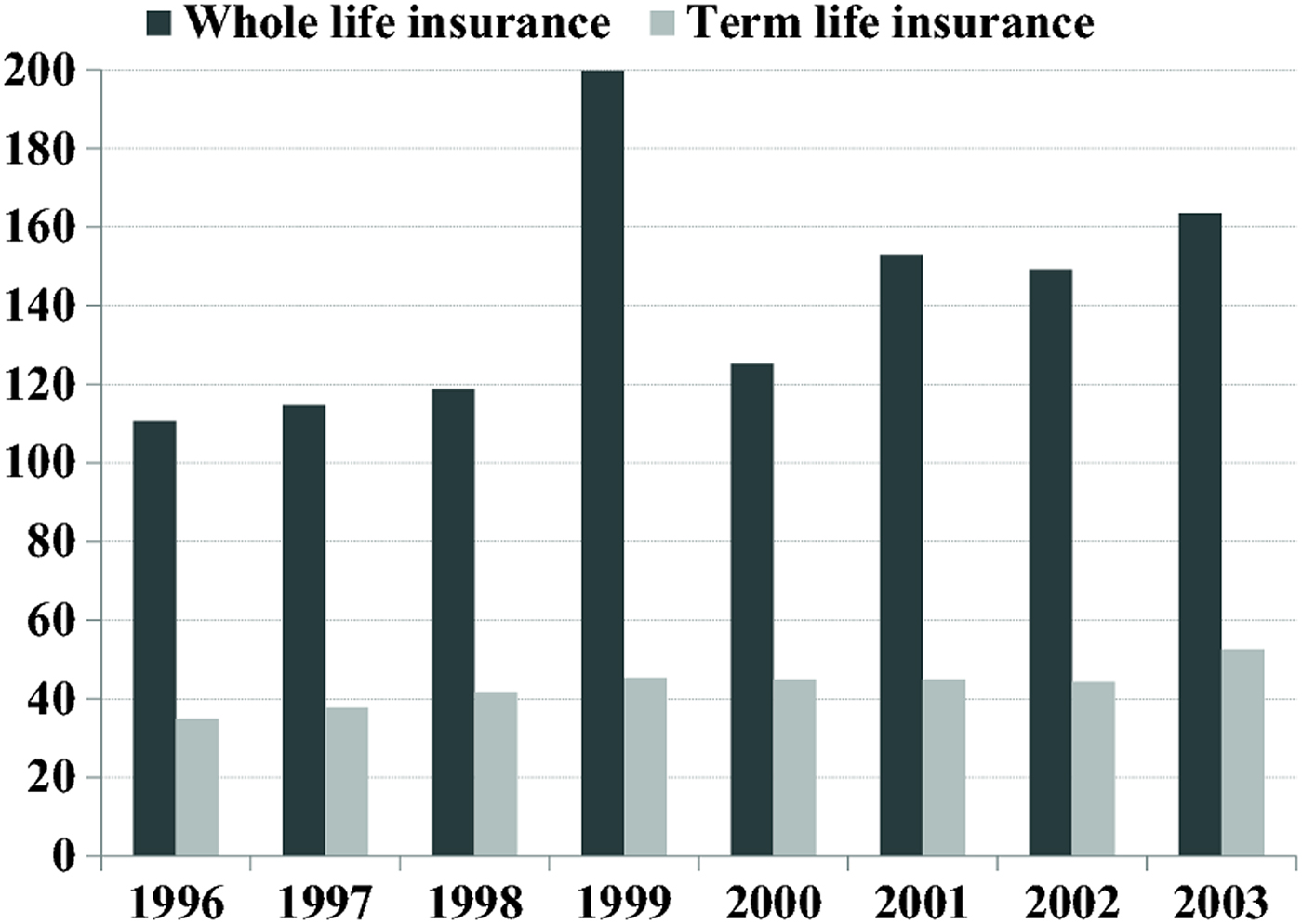
Households are asked annually if they owned one or more life insurance policies in the previous year. We therefore only use observations for households that take part in two successive surveys, with the dependent variable entering with a one period lead. As the survey does not contain any information on the nominal amount of life insurance purchased, we are only able to analyze changes in demand at the extensive margin. Moreover, the survey does unfortunately not distinguish between term and whole life insurance policies. This is not expected to significantly affect out estimates, however, for which the whole-life component is crucial, because whole life insurance is in general the dominant type in Germany, with term life policies only accounting for about one-quarter of all contracts at the time (GDV, 2003a and 2003b ). Moreover, at the macro-level, the ownership pattern and purchases of term life policies remained broadly stable during the period of observation (compare Figure 1). The survey contains similar yes/no questions for ownership of other assets such as savings accounts, stocks/mutual funds/bonds, building savings contracts, and business capital. However, information on households’ overall wealth or overall asset holdings is not available in the SOEP or in any other German microdata survey conducted during the relevant period.
(colour online) The graph depicts the insured volume of new term and whole life insurance contracts from 1996–2003 with first premium paid in billion euro in Germany. Whole life insurance comprises traditional contracts and contracts where the savings component of the life insurance contract is channeled into a mutual fund or pension plan. Source: GDV (2003b ).

As for the other covariates, it is noteworthy to describe the approximation of marginal tax rates, which is done in two steps. First, (estimated) tax payments, which are available in the SOEP, are transformed back into the household's taxable income, using the official tax formulas from the federal tax office that applied in each year.Footnote 8 Second, the household's marginal tax rate is calculated based on the derived taxable income and the marital status of the household. Socioeconomic characteristics are proxied by those of the household head.
In the next two sections, we use the analytic dataset constructed from the SOEP to analyze tax incentives and bequest motives, respectively.
6 Tax incentives
The unusually high popularity of life insurance in Germany is thought to be its favorable fiscal treatment (particularly of whole life insurance); see Sommer (Reference Sommer2007), inter alia. First, returns on life insurance are tax exempt if the contract lasts for at least 12 years, premiums are paid during at least 5 years, and the term life insurance component amounts to at least 60% of the total benefit paid out at the end of the contract. Second, annual contributions to whole life and term life insurance contracts are tax deductible. However, this is typically of little benefit for employees, as they reach the deductibility cap with their obligatory contributions to the social security system. Obligatory contributions are smaller for civil servants and the deductibility cap is higher for the self-employed, who are generally exempted from contributing to the public pension system and must provide for their own retirement income and survivor's benefits (Sommer, Reference Sommer2007). Our analysis includes controls for the self-employed and civil servants to account for these variations in effective deductibility. Finally, in the case of bequests, only two-thirds of the cash values of life insurance policies are taxed.
6.1 The reform of the tax exemption limit
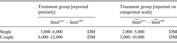
The German state taxes all personal interest and dividend income exceeding a certain threshold at the households’ marginal tax rate. The development of this threshold, the so-called Sparerfreibetrag (tax exemption limit), is shown in Table 1 for the period from 1996 to 2001. In March 1999, a law was passed, cutting the tax exemption limit from Deutsche Mark (DM) DM12,000 to DM6,000 for couples and DM6,000 to DM3,000 for singles from January 1, 2000 onward. We suspect that households between the old and the new tax exemption limits were disproportionately affected by this reform. As their interest and dividend income was fully exempted from taxation beforehand, the reform created a strong incentive to shelter their savings from taxation by purchasing whole life insurance when the reform was announced. In other words, if these households were responsive to the relative tax treatment, we should see a disproportionate increase of life insurance purchases among the group threatened to have their interest and dividend income taxed. In what follows, we denote households belonging to this category as the ‘treatment group’.
Tax exemption limits on interest and dividend income

Note: The tax exemption limit for interest and dividend income was cut to half in Germany in 2000. The table describes the treatment group, which are all households with interest and dividend income above the new and below the old tax exemption limit. The thresholds for singles for the old and new exemption limits, limit old = 6, 000 DM and limit new = 3, 000 DM (or twice these amounts for couples) define the treatment group. As survey respondents can either report their precise income or tick one of six pre-defined income ranges, the interest and dividend income for the latter can only be approximated from the categorical scale. About two-thirds of households chose to report their income on the categorical scale (indicated by tilde).
In order to identify the treatment group, we rely on a survey question that leaves it to the household whether to report its income from interest and dividends as the precise amount or within a range on an ordinal scale. Not surprisingly, three-quarters of households chose the ordinal response form, which offers ranges of less than 500, between 500 and 2,000, 2,000 and 5,000, 5,000 and 10,000, or above 10,000 DM. For these responses, we use the range between 2,000 and 5,000 DM to approximate households in the treatment group, or 5,000–10,000 DM in the case of married couples. While the ordinal thresholds may reduce the precision of the estimated response of the treatment group to tax changes, this attenuation bias will bias the results against finding significant differences between groups.Footnote 9
We use a difference-in-differences estimator to test if the treatment group is more likely to own one or more (tax-exempt) life insurance policies from 1999 onward. The choice of 1999 as reference year is motivated by the fact that the tax law was already passed in March 1999, so that households could anticipate the reform. Moreover, purchases were fostered by a parallel government proposal in June 1999, which wanted to abolish the tax exemption on life insurance returns altogether by the end of 1999. This second proposal eventually failed in the upper house of parliament (the Bundesrat) in mid-December, but was a strong driver of the anticipation effects until then.Footnote 10 Dolle-Helms (Reference Dolle-Helms1999a , Reference Dolle-Helms1999b ) provides anecdotal evidence that last minute purchases in 1999 were significant and largely driven by tax motives. The importance of anticipation effects is also confirmed by Figure 1, which shows the total insured volume of new whole and term life insurance contracts in Germany. While the value of term policies sold remains broadly stable over the entire sample, whole life insurance sales spike in 1999 and remain high thereafter. The sales of whole life contracts between 1996 and 1998 amount to an average insured volume of 115 billion Euro per year, while the average insured volume sold between 1999 and 2001 increased to 159 billion Euro.
Furthermore, the reform of the tax exemption limit may also have had an impact on households above the old exemption threshold, as their total taxable income from interest and dividends increased by the reduction in the exemption limit. These wealthy households should already have a tax incentive to buy life insurance before the reform, however. As the dependent variable does not allow distinguishing buyers of a second or third insurance policy, i.e., it does not measure changes at the intensive margin, we do not expect a significant response to the reform among this group of households. Still, we test if the ownership probability among the treatment group increases relative to households whose interest and dividend income already exceeded the old exemption limit. The implicit underlying identifying assumption is that both the treatment and the wealthy control group responded equally (in proportional terms) to the announcement of the reforms.
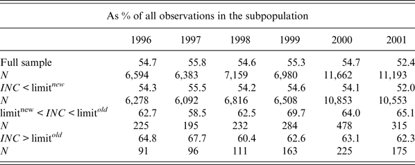
Descriptive statistics reported in Table 2 show that significant changes in life insurance ownership, i.e., at the extensive margin, occurred only in the treatment group. Life insurance ownership rates remained constant among households below the new tax exemption limit and above the old exemption limit. However, the ownership rate increased strongly from 62.5% to 69.7% in the treatment group in 1999 and remained at an elevated level thereafter. In line with the macro evidence, this indicates that households affected by the tax reform increased their life insurance demand in response to the tax reform, and largely anticipated their purchases in 1999 when the reform was announced.
Average life insurance ownership rates 1996–2001

Note: The table reports average ownership rates of life insurance policies for different subpopulations that are below, between or above the new and old tax exemption limits. INC denotes total interest and dividend income.
6.2 Unconditional estimates from a linear probability model
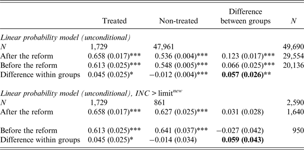
The upper panel of Table 3 reports the average effects of the tax reform, using a sample from 3 years before and after the announcement of the reform. While ownership rates of life insurance declined somewhat among households in the control group from 1999 onwards, an increase by 4.5% can be observed for the treatment group. The difference-in-differences estimate according to equation (9) is 5.7% for the full sample and statistically significant at the 5% confidence level. For households above the new exemption limit the estimate is of similar size, i.e., 5.9%. Due to the smaller sample size, however, the t-statistic does not indicate statistical significance at common confidence bounds.
Tax incentives – unconditional difference-in-differences estimates

Note: The upper panel reports average ownership rates of life insurance policies for the years 1996–2001. The bottom panel reports averages for all households with INC > limit new . The unconditional difference-in-differences estimate from a linear probability model based on equation (9) is reported in bold face in the bottom right cell of each panel. Standard errors are reported in parentheses and are clustered at the household level. *, **, *** denote statistical significance at the 10%, 5%, and 1% level, respectively.
6.3 Conditional estimates from a probit model
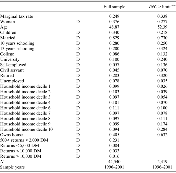
The probit model also controls for a number of additional covariates, whose summary statistics are reported in Table 4. In particular, we include the marginal tax rate to control for differences in after-tax returns. We proxy for the household's net labor income via binary indicators for deciles of the income distribution, suppressing the dummy for the median percentile.
Summary statistics

Note: The samples are from the SOEP. Demographic variables refer to the household head. Dummy variables are marked by D.
Dummies for house ownership as well as interest and dividend returns control for household wealth, where the lowest interest and dividend income category is suppressed (i.e., below DM500). Furthermore, binary indicators for marital status and households with one or more children living in the household are added to capture bequest motives as used for instance by Hurd (Reference Hurd1987, Reference Hurd1989). Dummies for employment status, civil servants, and the self-employed reflect specific characteristics of the German tax and public pension system. Finally, the model includes gender and education dummies, as well as linear and non-linear terms of the age of the household head. We use data for 3 years before and after the reform. The full sample consists of 44,540 observations and 2,419 if we constrain the analysis to households above the new exemption limit.
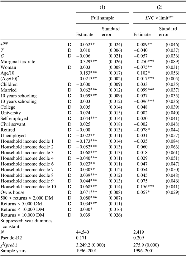
Table 5 reports average marginal effects for continuous and dummy variables. The interaction effect
 ${\hat \tau ^{DiD}}$
is statistically significant at the 5% level in both equations. According to equation (10), the reform increased ownership among households affected by the reduction of the tax exemption limit by 5.2%. The estimate is 8.9% for the restricted sample in column (2). These effects hold even after controlling for the marginal tax rate that applies to the household.
Tax incentives – conditional difference-in-differences estimates

The table reports estimates from a probit model that conditions on a large set of covariates. The treatment effect
 ${\hat \tau ^{DiD}}$
is estimated based on equation (10). Average marginal effects are reported. Robust and clustered standard errors are reported in parentheses. The right column runs the regression for a sub-sample of wealthy households above the new exemption limit, INC > limit
new
. D indicates dummy variables. ***, **, * indicate significance at the 0.01, 0.05, and 0.1 level, respectively.
Our results contrast with those of Jappelli and Pistaferri (Reference Jappelli and Pistaferri2003, Reference Jappelli and Pistaferri2007) who do not find that tax incentives matter for life-insurance demand in Italy. The authors mentioned that marketing efforts by Italian insurers did not sufficiently advertise the change in tax incentives following reforms in Italy. By contrast, anecdotal evidence suggests that sales agents exploited the favorable market situation in Germany deriving from the tax changes. Moreover, the tax incentive resulting from incremental changes in after-tax yields in Italy might have been too small to induce significant changes in investment behavior. In Germany, the reduction of the exemption limit implied that, on previously exempted interest and dividend income, some households could reduce their marginal tax rate of up to 51% in 2000 to 0% by rising the share of life insurance in their portfolios. The estimated effects should therefore be interpreted as local average treatment effects, as only a small group of rich households that are sensitive to exogenous changes in after-tax returns responded to the tax change. The Italian tax reform applied to a wider set of households, which may also explain the less pronounced sensitivity to the tax reform.
7 Bequest motives
From the theoretical model in Section 3, we derived two predictions with respect to bequests. First, a larger bequest motive raises demand for life insurance. Second, the response to tax changes is expected to be larger among households with stronger bequest motives.
When bringing these hypotheses of the model to the data, we face the problem that the SOEP provides asset ownership information only at the household level, whereas the theoretical model is developed in terms of a representative agent. It neither captures intra-household resource reallocation motives, nor is an overlapping generations model in which only children receive bequests. The set-up of the model allows for any person to be the beneficiary as long as it is stipulated in the insurance policy. Observing a larger response to the tax reform among households with children or married couples (i.e., those with potentially stronger bequest motives) would therefore be a sufficient test for the predictions of the model. However, when using a dummy for married couples as a proxy for bequest motives, some noise is introduced into the empirical specification, as all variables are observed at the household level while the theoretical model should in principle be applied to individuals, given that it does not explicitly deal with within couple resource allocation.
For the purpose at hand, however, it is not necessary to extend the model, as typical reasons for life insurance ownership of married couples can be interpreted as a larger η, i.e., stronger bequest incentives that are not related to other parameters of the model. Such reasons could for instance be income inequality within the household or estate tax incentives.Footnote 11 In order to ensure that the treatment effect for married households is estimated with sufficient precision, what is crucial is that both individuals within the household face the same tax rate. Such equalization of tax rates is ensured by the so-called income splitting mechanism of the German tax system.Footnote 12
Regarding the first hypothesis, we find that life insurance demand is higher for married couples but not for households with children.Footnote 13 The estimates in column (1) of Table 5 show that, ceteris paribus, married couples (who tend to have a higher preference for bequeathing wealth) have, on average, a 6.2% stronger demand for life insurance. By contrast, the presence of children seems not significantly related to life insurance demand, which has also been found by Jürges (Reference Jürges2001) based on SOEP data. One reason for this result could be that the indicator for households with children is an incomplete proxy variable that due to the nature of the questionnaire does not cover bequest motives to older children who do not live in the household anymore.
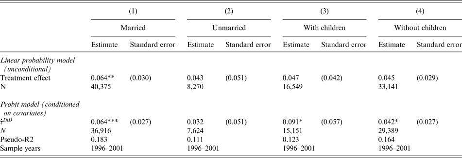
In addition to this mixed general evidence for the importance of bequest motives, Table 6 shows unconditional and conditional difference-in-differences estimates related to the second hypothesis on the impact of the tax reform on different groups of households. In particular, we compare the impact between married and unmarried households as well as households with and without children. Looking at the upper panel with unconditional difference-in-difference estimates, married households in the treatment group appear more likely to respond to the tax reform than unmarried households. The unconditional increase in life insurance ownership is statistically significant at 6.4% for married households. By contrast, no significant impact of the tax reform can be detected for the unmarried, and for households with or without children.Footnote 14
Bequest motives – average marginal effects

The upper panel reports unconditional difference-in-differences estimates of the treatment effect from a linear probability model based on equation (9). Estimates are reported for different sub-samples, i.e., married/unmarried couples and households with/without children. The bottom panel reports average marginal effects from a probit regression that conditions on a large number of other covariates. The treatment effect
 ${\hat \tau ^{DiD}}$
is estimated based on equation (10). Robust and clustered standard errors are reported in parentheses. ***, **, * indicate significance at the 0.01, 0.05, and 0.1 level, respectively.
Conditional estimates for the different sub-groups, based on equation (10), are reported in the lower panel of Table 6. The conditional probability of owning life insurance is 6.4% higher among married households affected by the tax reform. At the same time, we still find no statistically significant effect of the reform on unmarried households. This may indicate that the tax changes were not large enough to induce a change in life insurance among low-bequest households. Overall, the conditional effect of the tax reform for married households is of a similar magnitude as in the unconditional case.
For households with children, after controlling for other covariates, the estimated effect is larger than in the unconditional cases, with life insurance demand estimated to increase by 9.1% in response to the reform. Childless households increase their life insurance demand only by 4.2%, on average. However, for the case with children, it is noted that the estimates are only statistically significant at the 10% level.
8 Robustness checks
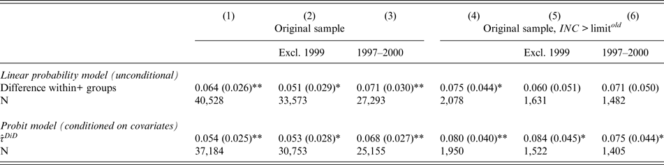
In order to assess the robustness of the estimates, we run several alternative specifications. One obvious source of concern is that the enlargement of the sample by about 3,500 households in 2000 biases the estimates and drives our findings. To control for this effect, we restrict the analysis solely to households from the original sample. Column (1) of Table 7 shows the estimated treatment effects for all households in the original sample. The unconditional estimate of 6.4% turns out to be of similar size as in the enlarged sample (5.7%), and is statistically significant at the 5% confidence level. Similarly, the conditional estimate is significant and of similar size as in the enlarged sample. Moreover, when we restrict the original sample to households above the new exemption limit, as is done in column (4), we also find statistically significant estimates with treatment effects of similar magnitude as for the enlarged sample, i.e., around 8%. We therefore conclude that the refreshment of the sample does not appear to bias our findings in a noteworthy manner.
Robustness checks – estimated treatment effects

Note: The table reports regression results for the original sample, not taking into account the enlargement of the survey sample in 2000. The difference-in-difference estimates are reported for different subsamples of the unconditioned linear probability model based on equation (9) and a probit model that conditions on a large set of covariates. For the probit model, the treatment effect
 ${\hat \tau ^{DiD}}$
is estimated based on equation (10). The sub-sample of wealthy households above the new exemption limit is denoted as INC >limit
new
. Standard errors are reported in parentheses and clustered at the household level.*, **, *** denote statistical significance at the 10%, 5% and 1% level, respectively.
As a next step, we want to rule out that our findings are solely driven by the strong increase in life insurance demand that was observed in 1999. In columns (2) and (5), observations for the year 1999 are therefore suppressed from the regressions. The estimates in column (2) show that, for both the unconditional and conditioned estimates neither the point estimates nor the standard errors change in a significant manner. However, when running the same exercise for the smaller sample of wealthy households, we cannot find a statistically significant effect for the unconditioned linear probability estimate anymore. Still, the conditioned probit estimate in the lower panel is similar to that from the full sample and also statistically significant.
Moreover, it is assessed if a narrower estimation window around the reform date would affect our conclusions. We therefore reduce the 3 to a 2 year estimation window ranging from 1997 to 2000. Column (3) shows that the estimates remain statistically significant and of similar size as in the wider estimation window, although the effects are estimated with less precision since standard errors increase. This effect is even more evident in the smaller sample of wealthy households. In column (6), estimates are only significant at the 10% level in the case of the conditional estimates and not significant anymore in the case of the unconditional estimates, although the point estimates are quite similar to those from the full sample. One explanation for this lower statistical significance is that the number of observations of wealthy households has nearly been halved by running the regressions on the narrower window compared with the enlarged sample.
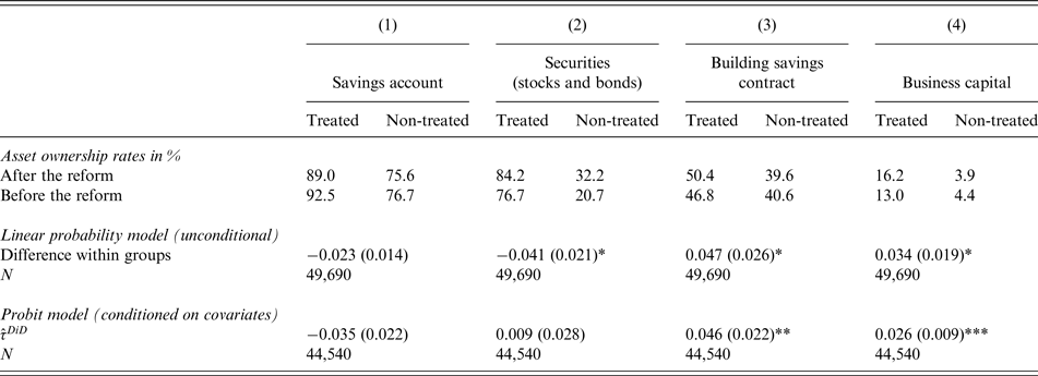
Finally, we explore if the estimated effect of the reform can only be established for life insurance ownership or is also observable for other asset groups. Variation in asset-specific sensitivities may reveal substitution among different assets, whereas a similar reaction across all assets could indicate that the treatment group reacted to the reform by increasing its overall saving. Hence, we estimate equations (9) and (10) by replacing the dependent variable with an indicator of ownership of: savings accounts, securities (not distinguishing between stocks and/or bonds), building savings contracts, and business capital in a company owned by a household member. Except for savings accounts, the other three assets also benefit of certain tax favors. For instance, building savings are tax deductible, and fringe benefits received in the form of building savings payments are exempt from taxation. Unincorporated business capital was traditionally taxed at the income tax rate, but in a move to promote investment, a parallel corporate tax reform in 2000 allowed individuals to have it taxed at the corporate tax rate, which is significantly lower. As for stocks, dividend payments are subject to regular income taxation, but at the time gains in the market value of the security were exempt from taxation if sale and purchase were at least 1 year apart, making long-term stock ownership attractive from a tax perspective.
Table 8 reports the estimated ownership rates broken down by treatment group as well as unconditional and conditional treatment effects. The treated group reduced participation in savings accounts and deposits from 93% before to 89% after the reform. However, this reduction is not statistically significant – which is not surprising as one would expect changes in the use of savings accounts in response to the tax reform at the intensive rather than the extensive margin. Securities ownership increased among the treated group but at a lesser rate than among the non-treated, resulting in a negative or insignificant treatment effect. This surprising finding should in our view not be over-interpreted, however as changes in stock ownership are likely driven by the privatization of the German telecommunications company Deutsche Telekom and the boom of the new economy stock market at the time. While both are aggregate phenomena that affected the treated and the non-treated, we suspect it invalidated the assumption of no group-specific trends which underlies the difference-in-differences model. Specifically, in an unprecedented advertising campaign on television, stock ownership was boosted particularly among households that had never owned stock before. This is evident in Table 8, which reports an increase in participation from 77% before to 84% after the reform among the treated (high wealth) households, while ownership rates of the non-treated (mainly low wealth) households surged from 21% to 32%.
Robustness checks – estimated treatment effects for other asset classes

Note: The table reports ownership rates households of affected and unaffected by the tax reform (i.e., treated and non-treated) for four different assets classes: savings accounts, securities, building savings contracts, and business capital. Three-year average ownership rates before (1996–1998) and after the reform (1999–2001) are reported in the top panel. The difference-in-difference estimates are reported for the unconditioned linear probability model based on equation (9) and a probit model that conditions on a large set of covariates. For the probit model, the treatment effect
 ${\hat \tau ^{DiD}}$
is estimated based on equation (10). Standard errors are reported in parentheses and clustered at the household level.*, **, *** denote statistical significance at the 10%, 5% and 1% level, respectively.
For building savings contracts and business capital, the treated show a significantly higher ownership rate after the reform. Like life insurance, both asset classes benefit of tax favors. Building savings contracts maintained a tax-favored treatment after the reform and the treated increased their participation at a roughly similar rate as for life insurance (around 10% of the pre-reform mean). We test if this similar response has implications for our findings on life insurance demand by controlling equation (10) also for ownership of building savings contracts. While there is some positive correlation between ownership of life insurance and building savings contracts, the estimated effect of the reform on life insurance ownership is not significantly different from the estimates reported in Table 5, with
 ${\hat \tau ^{DiD}}$
equal to 4.3% and statistically significant at the 5% level. For business capital, a favorable tax treatment was introduced with the corporate tax reform in 2000, but at the same time it should be noted that only around 5% of households in the overall sample own business capital, limiting the lessons that can be drawn from these estimates for the overall population.
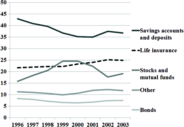
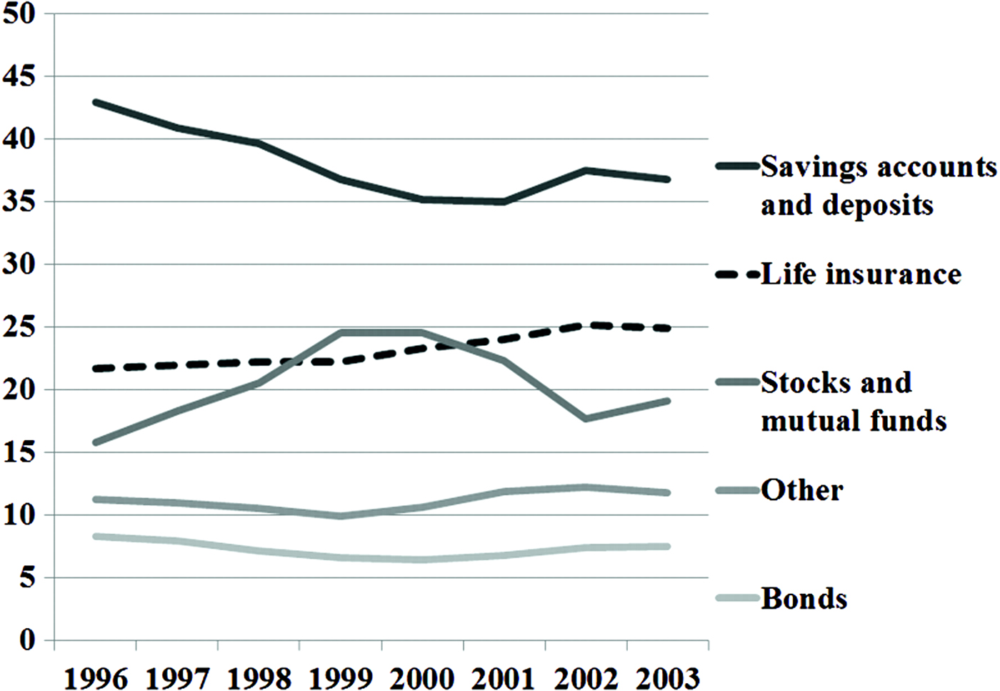
Overall, the estimated treatment effect on life insurance demand appears robust to a general trend among the treatment group, as some substitution can be observed into other asset classes, specifically from savings accounts into tax-favored assets. However, these estimates are only representative of effects at the extensive margin. Although these effects seem particularly relevant from a policy perspective, given their discrete nature and the possible presence of entry costs, they do not allow broader conclusions as to the implications of the reform on overall portfolio composition. An analysis of the latter would require data on overall savings that are unavailable in the SOEP. Nevertheless, some indication of changes in portfolio composition can be seen in macro-economic data. Figure 2 shows the share of different assets in total private wealth, as available from German financial accounts data. The share of life insurance wealth rises from 2000 onward, while the share of savings accounts and stocks declined.Footnote 15 The decline in stocks is likely driven by mark-to-market valuation changes following the bursting of the dotcom bubble, rather than active portfolio rebalancing, given that households are typically unwilling to realize losses. Therefore, we calculate the portfolio composition only for savings accounts/deposits, life insurance, and bonds, based on which it seems not too far-fetched to conclude that a portfolio shift from savings accounts towards life insurance occurred in response to the tax reform. While the share of life insurance in this three-asset portfolio rose by 4 percentage points to 36% between 1998 and 2003, the share of savings accounts declined by 4 percentage points to 53% over the same period. The share of bonds remained constant at 11%.
(colour online) The graph depicts the portfolio composition of German households between 1996 and 2003. The share of each asset class is reported as a percentage of total private wealth. The value of outstanding building savings contracts is included in savings and deposit account wealth. Source: Deutsche Bundesbank (2010).
9 Conclusions
Whole life insurance plays an important role in household saving. In a stylized model, both tax incentives and bequest motives drive whole life-insurance demand. While a bequest motive could be satisfied by term life insurance, sheltering savings from capital gains taxes is only possible with whole life policies. The empirical evidence we presented in this paper is consistent with the predictions of a stylized model that captures these incentives.
A tax reform that halved the tax exemption limit for interest and dividend income in Germany can be seen as a natural experiment. Underpinned by a rich dataset, this reform offers a rare opportunity to study the impact of increases in capital income taxation on portfolio choice. We find that the tax change induced a significant increase in ownership of tax-exempt assets. Participation in life insurance increased significantly among the group of households that did not pay taxes on interest and dividend income prior to the reform. Our difference-in-differences estimates imply that the tax reform we studied increased life insurance ownership probabilities by 5.2 percentage points among the group of households affected by the reform. We also tested if tax effects are larger among households with stronger bequest motives. Due to the tax change, demand at the extensive margin rises by 6.4% for married couples and 9.1% for households with children, which is larger than the respective response by unmarried and childless households.
These reduced-form estimates broadly support our theoretical model, thus indicating that bequests are indeed an important determinant of household savings decisions rather than an accidental remnant of precautionary saving (Hurd, Reference Hurd1987). As microdata on overall household saving, or on the amounts saved by asset type, are unavailable, it is not possible to ultimately establish whether increased participation in tax-favored assets occurred at the expense of other assets or whether it was driven by an increase in overall savings among those affected by the reform. However, we find that the treated also increased their participation in other tax-favored assets such as building savings contracts or business capital, while macro-economic financial accounts data suggests a portfolio shift from savings accounts into life insurance after the reform.
The estimated increase in life insurance participation in response to the tax change raises the question of whether a symmetric decline in life insurance ownership would be observed if the tax hike on regular savings were to be unwound in the future. From a theoretical perspective, the answer is clearly yes in the chosen setting, although in a more elaborate theoretical model with short-term liquidity constraints, the decline may turn out relatively smaller, as the shift of 1$ from life insurance to regular savings leads to a reduction in current resources for consumption in favor of future resources. Giving up current consumption may not be optimal for constrained households if the tax change were not expected to be permanent. More relevant from a practical point of view is that life insurance contracts can usually only be sold back to the insurance firm at a loss, as insurers keep potential excess gains on insurance reserves that would only be due at the contractual maturity. Since households will try to avoid realizing losses, overall life insurance ownership is likely to decline only gradually as contracts mature, while new sales are likely to adjust quickly. This reasoning is confirmed by the data. For example, Sauter and Winter (Reference Sauter and Winter2010) show descriptively that the eventual abolition of the tax advantage for life insurance in Germany in 2005 resulted in an immediate drop in sales of new contracts. By contrast, ownership rates declined only gradually from 52% in 2004 to 42% in 2011 according to the SOEP.
From a policy perspective, our results suggest that static tax revenue estimates, which do not account for participation responses to tax changes, may be misleading. Our findings show that these effects are potentially non-negligible. Thus, policy makers need to account for changes in investment behavior due to tax reforms, as forcefully argued by Poterba and Verdugo (Reference Poterba and Verdugo2011). In the light of the current concerns about fiscal sustainability in advanced economies, this could become relevant as governments seek new sources of revenues. Finally, our results show that increases in taxes on interest and dividend income may raise participation in tax-favored assets, such as life insurance policies. In that sense, an increase in these taxes may revive demand for life insurance in countries where they benefit from tax favors, despite the prevailing low interest rate environment.
Appendix
The solution for first period consumption c 0 can be derived as follows:
 $$\eqalign{{c_0} = & \left[ {\left( {1 + \displaystyle{1 \over R}{{(R{\eta _3})}^{\displaystyle{1 \over \gamma}}}} \right){{\left[ {\displaystyle{{{{({R^C} - R\alpha )}^2}\displaystyle{{{\pi _1}{\pi _2}} \over {1 + \delta}}} \over {(1 - {Z_0}R)(1 - {Z_1}R)}}} \right]}^{\displaystyle{1 \over \gamma}}}} \right. \cr & + \left( {\displaystyle{{{R^C} - \alpha R} \over {1 - {Z_1}R}}{Z_1} - \alpha} \right){\left( {\displaystyle{{(1 - {\pi _2}){\eta _2}\displaystyle{{{\pi _1}} \over {1 + \delta}} {{({R^C} - \alpha R)}^2}} \over {({Z_1}{R^C} - \alpha )(1 - {Z_0}R)}}} \right)^{\displaystyle{1 \over \gamma}}} \cr & + \left( {\displaystyle{{{R^C} - \alpha R} \over {1 - {Z_1}R}}} \right)\left( {{{\left( {\displaystyle{{({R^C} - \alpha R)\displaystyle{{{\pi _1}} \over {1 + \delta}}} \over {1 - {Z_0}R}}} \right)}^{\displaystyle{1 \over \gamma}}}} \right. \cr & + \left. {\left( {\displaystyle{{{R^C} - \alpha R} \over {1 - {Z_1}R}}{Z_1} - \alpha} \right){{\left( {\displaystyle{{(1 - {\pi _1}){\eta _1}({R^C} - \alpha R)} \over {{Z_0}{R^C} - \alpha}}} \right)}^{\displaystyle{1 \over \gamma}}}} \right) \cr & \times {\left. {\displaystyle{{{{({R^C} - \alpha R)}^2}} \over {(1 - {Z_0}R)(1 - {Z_1}R)}}} \right]^{ - 1}} \cr & \times \left[ {\displaystyle{{{{({R^C} - \alpha R)}^2}} \over {(1 - {Z_0}R)(1 - {Z_1}R)}}{w_0}(1 - {\tau ^S}) +} \right.\left. {\displaystyle{{{R^C} - \alpha R} \over {1 - {Z_1}R}}{w_1}(1 - {\tau ^S}) + {\tau ^S}({w_0}{G^2} + {w_1}G)} \right]} $$
The solution for c 0 in combination with equations (6)–(8) immediately implies values for c 1, c 2, b 1, b 2, b 3 and thus, by applying the budget constraints, also for L 1 and L 2.