1 Introduction
One of the most remarkable properties of viscoelastic fluids is the formation of instabilities at very low Reynolds numbers (Larson Reference Larson1992; Shaqfeh Reference Shaqfeh1996). Such instabilities are of a purely elastic nature; they occur when inertial forces are negligible and elastic forces are strong. In polymer solutions, elastic instabilities eventually lead to a chaotic regime known as elastic turbulence (Groisman & Steinberg Reference Groisman and Steinberg2000). The emergence of this regime is characterized by a fast growth of the Lyapunov exponent of the flow as the polymer elasticity exceeds a critical value (Burghelea, Segre & Steinberg Reference Burghelea, Segre and Steinberg2004). In addition, the kinetic-energy spatial and temporal spectra have a power-law behaviour, which indicates the presence of a large number of active scales in the flow. The spatial spectrum, however, is steeper than for Newtonian turbulence, i.e. velocity fluctuations are concentrated at small wavenumbers (Groisman & Steinberg Reference Groisman and Steinberg2000; Burghelea, Segre & Steinberg Reference Burghelea, Segre and Steinberg2007).
Elastic turbulence has important applications in microfluidics in view of the fact that it strongly enhances mixing in devices that, owing to their microscopic size, are characterized by a low Reynolds number (Groisman & Steinberg Reference Groisman and Steinberg2001). Moreover, the potential use of elastic turbulence in the oil industry has recently emerged as a promising application. Aqueous polymer solutions are indeed used to recover the oil that remains trapped inside the pores of reservoir rocks after an initial water flooding, and elastic turbulence has been proposed as a mechanism to explain the unexpectedly high efficiency of this oil recovery method (Mitchell et al. Reference Mitchell, Lyons, Howe and Clarke2016).
The simplest constitutive model of polymer solutions is the Oldroyd-B model (Oldroyd Reference Oldroyd1950), in which the dissolved polymer phase is described by a symmetric tensor field, termed the polymer-conformation tensor, which represents the moment of inertia of polymers averaged over thermal fluctuations. The Oldroyd-B model is thus a system of partial differential equations (PDEs) that describes the joint evolution of the velocity and the polymer-conformation tensor. In particular, the polymer feedback on the flow is given by a stress term proportional to the conformation tensor. The relevant dimensionless number is the Weissenberg number
 $Wi$
, i.e. the ratio of the polymer relaxation time and the typical time scale of the flow. The main limitation of this model is that it assumes linear polymer elasticity, which, in extensional flows and in the absence of polymer feedback, can lead to an unbounded growth of the conformation tensor and hence of polymer stresses.
In spite of its simplicity, the model successfully reproduces the main features of elastic turbulence (Fouxon & Lebedev Reference Fouxon and Lebedev2003; Berti et al. Reference Berti, Bistagnino, Boffetta, Celani and Musacchio2008; Berti & Boffetta Reference Berti and Boffetta2010; Grilli, Vázquez-Quesada & Ellero Reference Grilli, Vázquez-Quesada and Ellero2013). In particular, numerical simulations show that elastic turbulence is observed also in two-dimensional settings. It has attracted much attention in the mathematical community over the last two decades, during which analysts have focused on the existence, uniqueness and regularity of solutions (see, e.g., Lei, Masmoudi & Zhou Reference Lei, Masmoudi and Zhou2010; Barrett & Süli Reference Barrett and Süli2011; Constantin & Kliegl Reference Constantin and Kliegl2012; Elgindi & Rousset Reference Elgindi and Rousset2015; Hu & Lin Reference Hu and Lin2016, for some recent studies). To the best of our knowledge, there are few theoretical results on the properties of elastic turbulent solutions.
A mathematical definition of the number of degrees of freedom of a system of PDEs is given by the dimension of its global attractor (Robinson Reference Robinson2001). For the two-dimensional case, the bounds found by Constantin & Kliegl (Reference Constantin and Kliegl2012) on the
 $L^{2}$
-norms of the vorticity
 $\unicode[STIX]{x1D714}$
and the polymer-conformation tensor
 $\unicode[STIX]{x1D748}$
,
 $\Vert \unicode[STIX]{x1D714}\Vert _{2}$
and
 $\Vert \unicode[STIX]{x1D748}\Vert _{2}$
, are exponential in time (and double exponential for
 $\Vert \unicode[STIX]{x1D735}\unicode[STIX]{x1D748}\Vert _{2}$
). Thus, no bounded long-time averages
 $\langle \cdot \rangle$
have been found to exist, and, therefore, in a strictly rigorous sense, no global attractor is known to exist. Mathematically, we can go no further. However, numerical simulations of elastic turbulence (see § 4) suggest that
 $\Vert \unicode[STIX]{x1D714}\Vert _{2}$
,
 $\Vert \unicode[STIX]{x1D748}\Vert _{2}$
and
 $\Vert \unicode[STIX]{x1D735}\unicode[STIX]{x1D748}\Vert _{2}$
are indeed bounded in time for various values of
 $Wi$
. One practical way of progressing is to work under the following technical assumption with a subsequent strategy.
-
(i) Given that numerical calculations of
 $\Vert \unicode[STIX]{x1D714}\Vert _{2}$
,
$\Vert \unicode[STIX]{x1D748}\Vert _{2}$
and
$\Vert \unicode[STIX]{x1D735}\unicode[STIX]{x1D748}\Vert _{2}$
are finite in time, as suggested in § 4, we assume that a global attractor
${\mathcal{A}}$
exists.
-
(ii) Based on (i), we estimate the Lyapunov dimension of
${\mathcal{A}}$
, which will use the long-time averages
$\langle \Vert \unicode[STIX]{x1D714}\Vert _{2}\rangle$
,
$\langle \Vert \unicode[STIX]{x1D748}\Vert _{2}\rangle$
and
$\langle \Vert \unicode[STIX]{x1D735}\unicode[STIX]{x1D748}\Vert _{2}\rangle$
; the numerical bounds found in § 4 for these quantities in terms of
$Wi$
are used in our estimates.


A connection between the system dynamics and the attractor dimension is provided by the notion of the Lyapunov exponents via the Kaplan–Yorke formula. For ordinary differential equations (ODEs), the Lyapunov exponents control the exponential growth or contraction of volume elements in phase space, and the Kaplan–Yorke formula expresses the balance between volume growth and contraction realized on the attractor. The Kaplan–Yorke formula is used to define the Lyapunov dimension of the attractor and is as follows. For Lyapunov exponents
 $\unicode[STIX]{x1D707}_{1}\geqslant \unicode[STIX]{x1D707}_{2}\geqslant \cdots \geqslant \unicode[STIX]{x1D707}_{n}\geqslant \cdots \,$
, the Lyapunov dimension
 $d_{L}({\mathcal{A}})$
is given by
 $$\begin{eqnarray}d_{L}({\mathcal{A}})=N-1+\frac{\unicode[STIX]{x1D707}_{1}+\cdots +\unicode[STIX]{x1D707}_{N-1}}{-\unicode[STIX]{x1D707}_{N}},\end{eqnarray}$$
where the number
 $N$
of
 $\unicode[STIX]{x1D707}_{n}$
is chosen to satisfy
 $$\begin{eqnarray}\mathop{\sum }_{n=1}^{N-1}\unicode[STIX]{x1D707}_{n}\geqslant 0\quad \text{but}\quad \mathop{\sum }_{n=1}^{N}\unicode[STIX]{x1D707}_{n}<0.\end{eqnarray}$$
It should be noted that, according to the definition of
 $N$
, the ratio of exponents in (1.1) satisfies
 $$\begin{eqnarray}0\leqslant \frac{\unicode[STIX]{x1D707}_{1}+\cdots +\unicode[STIX]{x1D707}_{N-1}}{-\unicode[STIX]{x1D707}_{N}}<1.\end{eqnarray}$$
In simple terms, the value of
 $N$
that turns the sign of the sum of the Lyapunov exponents as in (1.2) is the value that bounds above
 $d_{L}({\mathcal{A}})$
such that
 $$\begin{eqnarray}N-1\leqslant d_{L}({\mathcal{A}})<N.\end{eqnarray}$$
The non-integer Lyapunov dimension
 $d_{L}({\mathcal{A}})$
generally bounds above the fractal and Hausdorff dimensions
 $d_{F}({\mathcal{A}})$
and
 $d_{H}({\mathcal{A}})$
. The Kaplan–Yorke formula originated as a phase-space argument for ODEs but has been rigorously applied to global attractors in PDEs by Constantin & Foias (Reference Constantin and Foias1985) (see also Gibbon & Titi Reference Gibbon and Titi1997). To use the method for PDEs to find an estimate for
 $d_{L}({\mathcal{A}})$
, it is necessary to extend the idea of the Lyapunov exponents to global Lyapunov exponents via a trace formula for the two-dimensional Oldroyd-B model that is explained in § 3. This uses the methods of Constantin & Foias (Reference Constantin and Foias1985), Constantin, Foias & Temam (Reference Constantin, Foias and Temam1988), Doering & Gibbon (Reference Doering and Gibbon1991) and, in particular, the
 $L^{\infty }$
-estimates of Constantin (Reference Constantin1987). For a two-dimensional system of side
 $L$
, the resolution length
 $\ell _{res}$
of the smallest feature in the dynamics is connected to
 $d_{L}({\mathcal{A}})$
by
 $d_{L}({\mathcal{A}})\sim (L/\ell _{res})^{2}$
.
2 The Oldroyd-B model for polymer solutions
On the periodic unit square
 $\unicode[STIX]{x1D6FA}=[0,\,1]^{2}$
, the dimensionless form of the Oldroyd-B model is
 $$\begin{eqnarray}\displaystyle & \displaystyle \unicode[STIX]{x2202}_{t}\boldsymbol{u}+\boldsymbol{u}\boldsymbol{\cdot }\unicode[STIX]{x1D735}\boldsymbol{u}=-\unicode[STIX]{x1D735}p+Re^{-1}\unicode[STIX]{x0394}\boldsymbol{u}+\unicode[STIX]{x1D6FD}(Wi\,Re)^{-1}\unicode[STIX]{x1D735}\boldsymbol{\cdot }\unicode[STIX]{x1D748}+\boldsymbol{F}, & \displaystyle\end{eqnarray}$$
 $$\begin{eqnarray}\displaystyle & \displaystyle \unicode[STIX]{x2202}_{t}\unicode[STIX]{x1D748}+\boldsymbol{u}\boldsymbol{\cdot }\unicode[STIX]{x1D735}\unicode[STIX]{x1D748}=(\unicode[STIX]{x1D735}\boldsymbol{u})\unicode[STIX]{x1D748}+\unicode[STIX]{x1D748}(\unicode[STIX]{x1D735}\boldsymbol{u})^{\top }-Wi^{-1}(\unicode[STIX]{x1D748}-\unicode[STIX]{x1D644})+Pe^{-1}\unicode[STIX]{x0394}\unicode[STIX]{x1D748}, & \displaystyle\end{eqnarray}$$
 $\boldsymbol{u}$
is the incompressible velocity field,
 $(\unicode[STIX]{x1D735}u)_{ij}=\unicode[STIX]{x2202}_{j}u_{i}$
,
 $\unicode[STIX]{x1D748}$
is the polymer-conformation tensor,
 $p$
is pressure, and where
 $Re$
,
 $Pe$
and
 $Wi$
are the Reynolds, Péclet and Weissenberg numbers respectively. The positive constant
 $\unicode[STIX]{x1D6FD}$
depends on the polymer concentration and equilibrium extension. The forcing
 $\boldsymbol{F}$
is time-independent, periodic and divergence-free (
 $\unicode[STIX]{x1D735}\boldsymbol{\cdot }\boldsymbol{F}=0$
).
The Laplacian term in (2.1b
) originates from the diffusion of the centre of mass of polymers (El-Kareh & Leal Reference El-Kareh and Leal1989), which ensures the global regularity of the two-dimensional Oldroyd-B model (Constantin & Kliegl Reference Constantin and Kliegl2012) and improves the stability of numerical simulations, even though the values of
 $Pe$
used in practice are considerably lower than its realistic values (Sureshkumar & Beris Reference Sureshkumar and Beris1995; Thomases Reference Thomases2011).
In two dimensions, (2.1) can be rewritten in terms of the scalar vorticity
 $\unicode[STIX]{x1D714}=\hat{\boldsymbol{z}}\boldsymbol{\cdot }(\unicode[STIX]{x1D735}\times \boldsymbol{u})$
:
 $$\begin{eqnarray}\displaystyle & \displaystyle \unicode[STIX]{x2202}_{t}\unicode[STIX]{x1D714}+\boldsymbol{u}\boldsymbol{\cdot }\unicode[STIX]{x1D735}\unicode[STIX]{x1D714}=Re^{-1}\unicode[STIX]{x0394}\unicode[STIX]{x1D714}+\unicode[STIX]{x1D6FD}(Wi\,Re)^{-1}\,\hat{\boldsymbol{z}}\boldsymbol{\cdot }\unicode[STIX]{x1D735}\times (\unicode[STIX]{x1D735}\boldsymbol{\cdot }\unicode[STIX]{x1D748})+f, & \displaystyle\end{eqnarray}$$
 $$\begin{eqnarray}\displaystyle & \displaystyle \unicode[STIX]{x2202}_{t}\unicode[STIX]{x1D748}+\boldsymbol{u}\boldsymbol{\cdot }\unicode[STIX]{x1D735}\unicode[STIX]{x1D748}=(\unicode[STIX]{x1D735}\boldsymbol{u})\unicode[STIX]{x1D748}+\unicode[STIX]{x1D748}(\unicode[STIX]{x1D735}\boldsymbol{u})^{\top }-Wi^{-1}(\unicode[STIX]{x1D748}-\unicode[STIX]{x1D644})+Pe^{-1}\unicode[STIX]{x0394}\unicode[STIX]{x1D748}, & \displaystyle\end{eqnarray}$$
 $f=\hat{\boldsymbol{z}}\boldsymbol{\cdot }(\unicode[STIX]{x1D735}\times \boldsymbol{F})$
and
 $\boldsymbol{u}=\unicode[STIX]{x1D735}^{\bot }\unicode[STIX]{x1D6E5}^{-1}\unicode[STIX]{x1D714}$
, with
 $\unicode[STIX]{x1D735}^{\bot }\equiv (-\unicode[STIX]{x2202}_{y},\unicode[STIX]{x2202}_{x})$
. Since
 $\boldsymbol{F}$
is periodic, the spatial average of
 $\unicode[STIX]{x1D714}$
is zero, and the inverse Laplacian of
 $\unicode[STIX]{x1D714}$
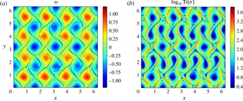
is properly defined. Figure 1 shows snapshots of the
 $\unicode[STIX]{x1D714}$
and
 $\text{Tr}\,\unicode[STIX]{x1D748}$
fields from a numerical simulation of (2.2) in the elastic-turbulence regime. It should be noted that
 $\text{Tr}\,\unicode[STIX]{x1D748}$
is concentrated over very thin regions, which is associated with large gradients in the polymer-conformation-tensor field.
Pseudocolour plot of (a)
 $\unicode[STIX]{x1D714}$
and (b)
 $\log _{10}\text{Tr}\,\unicode[STIX]{x1D748}$
for
 $Re=Re_{c}/\sqrt{2}$
,
 $Wi=20$
,
 $\unicode[STIX]{x1D6FD}=0.2$
and a cellular forcing with
 $n=4$
and
 $f_{0}=0.16$
(see § 4 for details).

3 Lyapunov dimension
In the PDE case, the phase space is now infinite-dimensional. We define
 $\boldsymbol{q}=(\unicode[STIX]{x1D714},\unicode[STIX]{x1D748})$
and denote by
 $\unicode[STIX]{x1D6FF}\boldsymbol{q}=(\unicode[STIX]{x1D6FF}\unicode[STIX]{x1D714},\unicode[STIX]{x1D6FF}\unicode[STIX]{x1D748})$
the infinitesimal displacement about
 $\boldsymbol{q}$
;
 $\unicode[STIX]{x1D6FF}\boldsymbol{q}$
satisfies the linearized set of equations from (2.2):
 $$\begin{eqnarray}\displaystyle & & \displaystyle \unicode[STIX]{x1D6FF}\dot{\boldsymbol{q}}=\unicode[STIX]{x1D63C}(t)\unicode[STIX]{x1D6FF}\boldsymbol{q}\nonumber\\ \displaystyle & & \displaystyle \quad =\left(\begin{array}{@{}c@{}}-\boldsymbol{u}\boldsymbol{\cdot }\unicode[STIX]{x1D735}\unicode[STIX]{x1D6FF}\unicode[STIX]{x1D714}+{\displaystyle \frac{1}{Re}}\unicode[STIX]{x0394}\unicode[STIX]{x1D6FF}\unicode[STIX]{x1D714}-\unicode[STIX]{x1D6FF}\boldsymbol{u}\boldsymbol{\cdot }\unicode[STIX]{x1D735}\unicode[STIX]{x1D714}+{\displaystyle \frac{\unicode[STIX]{x1D6FD}}{Wi\,Re}}\hat{\boldsymbol{z}}\boldsymbol{\cdot }\unicode[STIX]{x1D735}\times (\unicode[STIX]{x1D735}\boldsymbol{\cdot }\unicode[STIX]{x1D6FF}\unicode[STIX]{x1D748})\\ (\unicode[STIX]{x1D735}\unicode[STIX]{x1D6FF}\boldsymbol{u})\unicode[STIX]{x1D748}+\unicode[STIX]{x1D748}(\unicode[STIX]{x1D735}\unicode[STIX]{x1D6FF}\boldsymbol{u})^{\top }-\unicode[STIX]{x1D6FF}\boldsymbol{u}\boldsymbol{\cdot }\unicode[STIX]{x1D735}\unicode[STIX]{x1D748}-\boldsymbol{u}\boldsymbol{\cdot }\unicode[STIX]{x1D735}\unicode[STIX]{x1D6FF}\unicode[STIX]{x1D748}+(\unicode[STIX]{x1D735}\boldsymbol{u})\unicode[STIX]{x1D6FF}\unicode[STIX]{x1D748}+\unicode[STIX]{x1D6FF}\unicode[STIX]{x1D748}(\unicode[STIX]{x1D735}\boldsymbol{u})^{\top }-{\displaystyle \frac{\unicode[STIX]{x1D6FF}\unicode[STIX]{x1D748}}{Wi}}+{\displaystyle \frac{1}{Pe}}\unicode[STIX]{x0394}\unicode[STIX]{x1D6FF}\unicode[STIX]{x1D748}\end{array}\right),\nonumber\\ \displaystyle & & \displaystyle\end{eqnarray}$$
where the explicit form of the operator
 $\unicode[STIX]{x1D63C}(t)$
is obtained by using
 $\boldsymbol{u}=\unicode[STIX]{x1D735}^{\bot }\unicode[STIX]{x1D6E5}^{-1}\unicode[STIX]{x1D714}$
to express
 $\boldsymbol{u}$
and
 $\unicode[STIX]{x1D6FF}\boldsymbol{u}$
in terms of
 $\unicode[STIX]{x1D714}$
and
 $\unicode[STIX]{x1D6FF}\unicode[STIX]{x1D714}$
respectively. Following Constantin & Foias (Reference Constantin and Foias1985), we take different sets of initial conditions
 $\boldsymbol{q}(0)+\unicode[STIX]{x1D6FF}\boldsymbol{q}_{i}(0)$
which evolve into
 $\boldsymbol{q}(t)+\unicode[STIX]{x1D6FF}\boldsymbol{q}_{i}(t)$
for
 $i=1,\ldots ,N$
. If they are chosen to be linearly independent, these
 $\unicode[STIX]{x1D6FF}\boldsymbol{q}_{i}$
form an
 $N$
-volume or parallelepiped of volume
 $V_{N}(t)=|\unicode[STIX]{x1D6FF}\boldsymbol{q}_{1}\wedge \unicode[STIX]{x1D6FF}\boldsymbol{q}_{2}\cdots \wedge \unicode[STIX]{x1D6FF}\boldsymbol{q}_{N}|,$
which changes along the solution
 $\boldsymbol{q}(t)$
, so we need to find its time evolution. This is given by
 $\dot{V}_{N}=V_{N}\text{Tr}[\unicode[STIX]{x1D63C}\unicode[STIX]{x1D64B}_{N}]$
, which is easily solved to give
 $$\begin{eqnarray}V_{N}(t)=V_{N}(0)\exp \left\{\int _{0}^{t}\text{Tr}[\unicode[STIX]{x1D63C}\unicode[STIX]{x1D64B}_{N}](\unicode[STIX]{x1D70F})\,\text{d}\unicode[STIX]{x1D70F}\right\},\end{eqnarray}$$
where
 $\unicode[STIX]{x1D64B}_{N}(t)$
is an
 $L^{2}$
-orthogonal projection onto the finite-dimensional subspace
 $\text{span}\,\{\unicode[STIX]{x1D6FF}\boldsymbol{q}_{1},\unicode[STIX]{x1D6FF}\boldsymbol{q}_{2},\ldots ,\unicode[STIX]{x1D6FF}\boldsymbol{q}_{N}\}$
. In terms of the time average
 $\langle \cdot \rangle$
, the sum of the first
 $N$
global Lyapunov exponents is taken to be (Constantin & Foias Reference Constantin and Foias1985)
 $$\begin{eqnarray}\mathop{\sum }_{n=1}^{N}\unicode[STIX]{x1D707}_{n}=\langle \text{Tr}[\unicode[STIX]{x1D63C}\unicode[STIX]{x1D64B}_{N}]\rangle .\end{eqnarray}$$
To estimate the Lyapunov dimension, we wish to find the value of
 $N$
that turns the sign of
 $\langle \text{Tr}[\unicode[STIX]{x1D63C}\unicode[STIX]{x1D64B}_{N}]\rangle$
. This value of
 $N$
bounds above
 $d_{L}({\mathcal{A}})$
as in (1.4). As we are interested in elastic turbulence, we assume
 $Pe\gg 1$
,
 $Wi\gg 1$
and
 $0<Re<Re_{c}$
, where
 $Re_{c}$
is the critical value for the appearance of inertial instabilities. The derivation has been relegated to appendix A. The final result is that the following inequalities are sufficient conditions on
 $N$
for the growth rate
 $\langle \text{Tr}[\unicode[STIX]{x1D63C}\unicode[STIX]{x1D64B}_{N}]\rangle$
to be negative and the
 $N$
-volume
 $V_{N}$
to contract:
 $$\begin{eqnarray}\displaystyle & \displaystyle N>cRe\langle \Vert \unicode[STIX]{x1D748}\Vert _{2}^{3}\rangle ^{1/3}(1+\ln Re+\ln \langle \Vert \unicode[STIX]{x1D748}\Vert _{2}^{3}\rangle ^{1/3})^{1/2}, & \displaystyle\end{eqnarray}$$
 $$\begin{eqnarray}\displaystyle & \displaystyle N>cRe^{2/3}\langle \Vert \unicode[STIX]{x1D735}\unicode[STIX]{x1D748}\Vert _{2}^{2}\rangle ^{1/3}(1+\ln Re+\ln \langle \Vert \unicode[STIX]{x1D735}\unicode[STIX]{x1D748}\Vert _{2}^{2}\rangle ^{1/2})^{1/3}, & \displaystyle\end{eqnarray}$$
 $\Vert \cdot \Vert _{2}^{2}=\int _{\unicode[STIX]{x1D6FA}}|\cdot |^{2}\,\text{d}\boldsymbol{x}$
,
 $|\unicode[STIX]{x1D748}|^{2}=\sum _{i,j}|\unicode[STIX]{x1D70E}_{ij}|^{2}$
,
 $|\unicode[STIX]{x1D735}\unicode[STIX]{x1D748}|^{2}=\sum _{i,j,k}|\unicode[STIX]{x2202}_{k}\unicode[STIX]{x1D70E}_{ij}|^{2}$
and
 $c$
is regarded as a generic positive dimensionless constant. These conditions depend on estimates for
 $\langle \Vert \unicode[STIX]{x1D748}\Vert _{2}^{3}\rangle$
and
 $\langle \Vert \unicode[STIX]{x1D735}\unicode[STIX]{x1D748}\Vert _{2}^{2}\rangle$
. It has been shown in Constantin & Kliegl (Reference Constantin and Kliegl2012) that these are exponential in time and thus cannot be used. Instead, we turn to direct numerical simulations to find their behaviour in terms of
 $Wi$
.
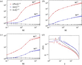
Plot of
 $\langle \Vert \unicode[STIX]{x1D714}\Vert _{2}^{2}\rangle ^{1/2}$
(black squares),
 $\langle \Vert \unicode[STIX]{x1D748}\Vert _{2}^{3}\rangle ^{1/3}$
(blue circles) and
 $\langle \Vert \unicode[STIX]{x1D735}\unicode[STIX]{x1D748}\Vert _{2}^{2}\rangle ^{1/3}$
(red triangles) as a function of
 $Wi$
for
 $Re=Re_{c}/\sqrt{2}$
,
 $\unicode[STIX]{x1D6FD}=0.2$
, and (a) cellular forcing with
 $n=4$
,
 $f_{0}=0.16$
, (b) cellular forcing with
 $n=10$
,
 $f_{0}=2.50$
and (c) Kolmogorov forcing with
 $n=8$
,
 $f_{0}=1.28$
. (d) Kinetic-energy spectrum for
 $Wi=20$
for case (a) in red, case (b) in blue and case (c) in black. The spectrum shows a power-law behaviour
 $E(k)\simeq k^{-a}$
with
 $a\approx 3.1$
for case (a),
 $a\approx 3.0$
for case (b) and
 $a\approx 3.7$
for case (c).

4 Direct numerical simulations of elastic turbulence
To simulate solutions of (2.2), we use the approach described in Gupta, Perlekar & Pandit (Reference Gupta, Perlekar and Pandit2015) and Gupta & Pandit (Reference Gupta and Pandit2017). For the time integration, we use the fourth-order Runge–Kutta scheme with time step
 $\unicode[STIX]{x1D6FF}t=10^{-4}$
, while the fourth-order central-finite-difference scheme with
 $1024^{2}$
collocation points is employed for the spatial derivatives. To accurately resolve the steep gradients of
 $\unicode[STIX]{x1D748}$
, we apply the Kurganov–Tadmor scheme to the advection term in (2.2b
) (Kurganov & Tadmor Reference Kurganov and Tadmor2000) (see Vaithianathan et al.
Reference Vaithianathan, Robert, Brasseur and Collins2006, for the application of this scheme to viscoelastic fluids), which allows us to set
 $Pe=\infty$
in (2.2). The velocity is calculated from the vorticity via the Poisson equation
 $\unicode[STIX]{x0394}\unicode[STIX]{x1D713}=\unicode[STIX]{x1D714}$
, where
 $\unicode[STIX]{x1D713}$
is the stream function:
 $\boldsymbol{u}=\unicode[STIX]{x1D735}^{\bot }\unicode[STIX]{x1D713}$
. The pseudospectral method is used to solve the Poisson equation in Fourier space. The simulations were performed on
 $[0,2\unicode[STIX]{x03C0}]^{2}$
and the solutions were rescaled appropriately.
Three kinds of forcing are considered: a cellular forcing
 $f=-f_{0}n[\cos (nx)+\cos (ny)]$
with
 $n=4$
, a cellular forcing with
 $n=10$
and a Kolmogorov forcing
 $f=-f_{0}n\cos (nx)$
with
 $n=8$
. In all simulations,
 $Re=Re_{c}/\sqrt{2}$
, where
 $Re_{c}$
is the critical Reynolds number above which inertial instabilities occur. Hence, in the absence of polymers (
 $\unicode[STIX]{x1D6FD}=0$
), the stationary vorticity field shows alternating vortices and antivortices for the cellular forcing and a parallel sinusoidal flow for the Kolmogorov forcing. The parameter
 $\unicode[STIX]{x1D6FD}$
is set to
 $\unicode[STIX]{x1D6FD}=0.2$
. We checked that in the elastic-turbulence regime, the kinetic-energy transfer due to the fluid inertia is negligible, so the chaotic dynamics is entirely due to polymer stresses.
The numerical simulations show that
 $\langle \Vert \unicode[STIX]{x1D735}\unicode[STIX]{x1D748}\Vert _{2}^{2}\rangle ^{1/3}$
is greater than
 $\langle \Vert \unicode[STIX]{x1D748}\Vert _{2}^{3}\rangle ^{1/3}$
, and, at large
 $Wi$
,
 $\langle \Vert \unicode[STIX]{x1D735}\unicode[STIX]{x1D748}\Vert _{2}^{2}\rangle ^{1/3}\sim Wi^{\unicode[STIX]{x1D6FC}}$
with
 $\unicode[STIX]{x1D6FC}\approx 0.7$
for the three different forcings considered here (see figure 2). This result is in agreement with the observation of large gradients in the polymer-conformation field in figure 1 as well as in previous numerical simulations (Berti et al.
Reference Berti, Bistagnino, Boffetta, Celani and Musacchio2008; Berti & Boffetta Reference Berti and Boffetta2010). It follows that the value of
 $N$
such that
 $N$
-volumes contract is determined by inequality (3.4b
). We conclude that, in the elastic-turbulence regime and under the specified assumptions, the two-dimensional Oldroyd-B model has a finite-dimensional global attractor with Lyapunov dimension
 $$\begin{eqnarray}d_{L}({\mathcal{A}})\leqslant {\mathcal{N}},\end{eqnarray}$$
where
 ${\mathcal{N}}$
is the minimum value of
 $N$
satisfying (3.4b
). Thus, up to logarithmic corrections,
 $$\begin{eqnarray}d_{L}({\mathcal{A}})\lesssim cRe^{2/3}\langle \Vert \unicode[STIX]{x1D735}\unicode[STIX]{x1D748}\Vert _{2}^{2}\rangle ^{1/3}\sim CWi^{\unicode[STIX]{x1D6FC}},\end{eqnarray}$$
where
 $\unicode[STIX]{x1D6FC}\approx 0.7$
and
 $C$
depends on
 $Re$
. We have also performed numerical simulations at smaller values of
 $Re$
, which indicate that
 $\unicode[STIX]{x1D6FC}$
does not depend on
 $Re$
. It is worth noting that since
 $\Vert \unicode[STIX]{x1D735}\unicode[STIX]{x1D748}\Vert$
grows with
 $Wi$
, inequality (3.4) implies that a lower
 $Re$
requires a higher
 $Wi$
to obtain the same attractor dimension. This is in agreement with the stability analysis of the Oldroyd-B model, according to which the critical
 $Wi$
for the appearance of elastic instabilities increases as
 $Re$
decreases (e.g. Larson Reference Larson1992; Boffetta et al.
Reference Boffetta, Celani, Mazzino, Puliafito and Vergassola2005).
5 Conclusions
Through a mathematical and numerical analysis of the two-dimensional Oldroyd-B model in the elastic-turbulence regime, we have made a practical estimate of the dimension of its (assumed) global attractor, as suggested by numerical simulations. We have also shown that the complexity of the attractor is related to the formation of large gradients in the polymer-conformation field. Although the asymptotic power-law dependence of
 $d_{L}({\mathcal{A}})$
on
 $Wi$
was found to be the same for different forcings, further studies are required to confirm the potential universality of the exponent
 $\unicode[STIX]{x1D6FC}$
.
As mentioned in the introduction, the main limitation of the Oldroyd-B model is the absence of a maximum polymer elongation. Other constitutive models of polymer solutions, such as the FENE-P model, overcome this limitation by introducing a nonlinear elastic force that diverges when
 $\text{Tr}\,\unicode[STIX]{x1D748}$
approaches the square of the maximum elongation (see Thomases, Shelley & Thiffeault Reference Thomases, Shelley and Thiffeault2011; Gupta & Pandit Reference Gupta and Pandit2017, for the application of the FENE-P model to the study of elastic turbulence). However, the use of a nonlinear elastic force does not prevent the formation of large gradients in the
 $\unicode[STIX]{x1D748}$
-field (Thomases, Shelley & Thiffeault Reference Thomases, Shelley and Thiffeault2011). In other words, large values of
 $\unicode[STIX]{x1D735}\unicode[STIX]{x1D748}$
seem to occur independently of the form of the force that describes the elasticity of polymers. Our estimate (4.2) depends on
 $\Vert \unicode[STIX]{x1D735}\unicode[STIX]{x1D748}\Vert _{2}$
rather than
 $\Vert \unicode[STIX]{x1D748}\Vert _{2}$
. This fact suggests that, albeit based on the Oldroyd-B model, (4.2) may also be relevant to other constitutive models.
Our analysis can be adapted to the Oldroyd-B model coupled with the unsteady Stokes equations, in which the
 $\boldsymbol{u}\boldsymbol{\cdot }\unicode[STIX]{x1D735}\boldsymbol{u}$
term is set to zero; the estimates for
 $N$
given in (3.4) are unchanged. The
 $Re=0$
case, in which (2.1a
) is replaced with the Stokes equations (Thomases & Shelley Reference Thomases and Shelley2009; Thomases et al.
Reference Thomases, Shelley and Thiffeault2011), would require, by contrast, a separate analysis, because
 $\unicode[STIX]{x1D714}$
would depend on
 $\unicode[STIX]{x1D748}$
via a time-independent differential relation and (2.2) would reduce to a dynamical system in the
 $\unicode[STIX]{x1D748}$
-space only. It would also be interesting to explore whether or not a relation exists between the exponent
 $\unicode[STIX]{x1D6FC}$
in (4.2) and the exponent of the singular structures that emerge near hyperbolic points in the
 $Re=0$
case (Renardy Reference Renardy2006; Thomases & Shelley Reference Thomases and Shelley2007).
Elastic turbulence is observed at low
 $Re$
and high
 $Wi$
. When both
 $Re$
and
 $Wi$
are high, the addition of polymers to a two-dimensional turbulent flow suppresses large-scale velocity fluctuations (Amarouchene & Kellay Reference Amarouchene and Kellay2002). This phenomenon is once again correctly reproduced by the Oldroyd-B model (Boffetta, Celani & Musacchio Reference Boffetta, Celani and Musacchio2003). Our estimate (A 18), which gives a sufficient condition for the contraction of
 $N$
-volumes, holds for all values of
 $Re$
. It would be interesting to investigate the implications of this estimate for the attractor dimension in the high-
 $Re$
regime.
Acknowledgements
The authors would like to acknowledge useful discussions with G. Boffetta, A. Mazzino, S. Musacchio, P. Perlekar and S. S. Ray. The work of E.L.C.M.P. was supported by EACEA through the EMMA program. E.L.C.M.P. and D.V. acknowledge the support of the EU COST Action MP 1305 ‘Flowing Matter.’ The authors also acknowledge the Observatoire de la Côte d’Azur for computing resources.
Appendix A. Derivation of the decay rate of
$N$
-dimensional volumes

Here, we show the main steps needed to obtain (3.4). The trace
 $\text{Tr}[\unicode[STIX]{x1D63C}\unicode[STIX]{x1D64B}_{N}]$
can be expressed as (e.g. Constantin & Foias Reference Constantin and Foias1985; Doering & Gibbon Reference Doering and Gibbon1995; Robinson Reference Robinson2001)
 $$\begin{eqnarray}\text{Tr}[\unicode[STIX]{x1D63C}\unicode[STIX]{x1D64B}_{N}]=\mathop{\sum }_{n=1}^{N}\int _{\unicode[STIX]{x1D6FA}}\unicode[STIX]{x1D731}_{n}\boldsymbol{\cdot }\unicode[STIX]{x1D63C}\unicode[STIX]{x1D731}_{n}\,\text{d}\boldsymbol{x},\end{eqnarray}$$
where
 $\{\unicode[STIX]{x1D731}_{n}\}_{n=1}^{N}=\{(\unicode[STIX]{x1D719}_{n}^{\unicode[STIX]{x1D714}},\unicode[STIX]{x1D753}_{n}^{\unicode[STIX]{x1D70E}})\}_{n=1}^{N}$
is an orthonormal set spanning the subspace generated by the displacements
 $\{(\unicode[STIX]{x1D6FF}\unicode[STIX]{x1D714}_{n},\unicode[STIX]{x1D6FF}\unicode[STIX]{x1D748}_{n})\}_{n=1}^{N}$
and where
 $\{\unicode[STIX]{x1D719}_{n}^{\unicode[STIX]{x1D714}}\}_{n=1}^{N}$
is such that
 $\int _{\unicode[STIX]{x1D6FA}}\unicode[STIX]{x1D719}_{n}^{\unicode[STIX]{x1D714}}\unicode[STIX]{x1D719}_{m}^{\unicode[STIX]{x1D714}}\,\text{d}\boldsymbol{x}=0$
if
 $n\neq m$
, and
 $\{\unicode[STIX]{x1D753}_{n}^{\unicode[STIX]{x1D70E}}\}_{n=1}^{N}$
with
 $(\unicode[STIX]{x1D753}_{n}^{\unicode[STIX]{x1D70E}})^{\top }=\unicode[STIX]{x1D753}_{n}^{\unicode[STIX]{x1D70E}}$
is such that
 $\int _{\unicode[STIX]{x1D6FA}}\unicode[STIX]{x1D753}_{n}^{\unicode[STIX]{x1D70E}}:\unicode[STIX]{x1D753}_{m}^{\unicode[STIX]{x1D70E}}\,\text{d}\boldsymbol{x}=0$
if
 $n\neq m$
. The orthonormality of
 $\{\unicode[STIX]{x1D731}_{n}\}_{n=1}^{N}$
should then be interpreted as follows:
 $\int _{\unicode[STIX]{x1D6FA}}\unicode[STIX]{x1D719}_{m}^{\unicode[STIX]{x1D714}}\unicode[STIX]{x1D719}_{n}^{\unicode[STIX]{x1D714}}\,\text{d}\boldsymbol{x}+\int _{\unicode[STIX]{x1D6FA}}\unicode[STIX]{x1D753}_{m}^{\unicode[STIX]{x1D70E}}:\unicode[STIX]{x1D753}_{n}^{\unicode[STIX]{x1D70E}}\,\text{d}\boldsymbol{x}=\unicode[STIX]{x1D6FF}_{mn},$
whence
 $$\begin{eqnarray}\mathop{\sum }_{n=1}^{N}\int _{\unicode[STIX]{x1D6FA}}|\unicode[STIX]{x1D731}_{n}|^{2}\,\text{d}\boldsymbol{x}=\mathop{\sum }_{n=1}^{N}\int _{\unicode[STIX]{x1D6FA}}(|\unicode[STIX]{x1D719}_{n}^{\unicode[STIX]{x1D714}}|^{2}+|\unicode[STIX]{x1D753}_{n}^{\unicode[STIX]{x1D70E}}|^{2})\,\text{d}\boldsymbol{x}=N.\end{eqnarray}$$
The symbol ‘:’ denotes the inner product between matrices,
 $\unicode[STIX]{x1D748}:\unicode[STIX]{x1D748}^{\prime }\equiv \text{Tr}[\unicode[STIX]{x1D748}^{\top }\unicode[STIX]{x1D748}^{\prime }]$
. The following inequality (e.g. Robinson Reference Robinson2001) will also be used when we estimate the norms of
 $\unicode[STIX]{x1D719}_{n}^{\unicode[STIX]{x1D714}},\unicode[STIX]{x1D753}_{n}^{\unicode[STIX]{x1D70E}}$
or of their gradients:
 $$\begin{eqnarray}\unicode[STIX]{x1D6E9}\equiv \text{Tr}[-\unicode[STIX]{x0394}\unicode[STIX]{x1D64B}_{N}]=-\mathop{\sum }_{n=1}^{N}\int _{\unicode[STIX]{x1D6FA}}(\unicode[STIX]{x1D719}_{n}^{\unicode[STIX]{x1D714}}\unicode[STIX]{x0394}\unicode[STIX]{x1D719}_{n}^{\unicode[STIX]{x1D714}}+\unicode[STIX]{x1D753}_{n}^{\unicode[STIX]{x1D70E}}:\unicode[STIX]{x0394}\unicode[STIX]{x1D753}_{n}^{\unicode[STIX]{x1D70E}})\,\text{d}\boldsymbol{x}\geqslant cN^{2}.\end{eqnarray}$$
The terms appearing in (A 1) can be explicitly listed as (the terms that follow from
 $\boldsymbol{u}\boldsymbol{\cdot }\unicode[STIX]{x1D735}\unicode[STIX]{x1D6FF}\unicode[STIX]{x1D714}$
and
 $\boldsymbol{u}\boldsymbol{\cdot }\unicode[STIX]{x1D735}\unicode[STIX]{x1D6FF}\unicode[STIX]{x1D748}$
vanish because of the incompressibility of
 $\boldsymbol{u}$
)
 $$\begin{eqnarray}\displaystyle & & \displaystyle \text{Tr}[\unicode[STIX]{x1D63C}\unicode[STIX]{x1D64B}_{N}]=Re^{-1}\mathop{\sum }_{n=1}^{N}\int _{\unicode[STIX]{x1D6FA}}\unicode[STIX]{x1D719}_{n}^{\unicode[STIX]{x1D714}}\unicode[STIX]{x0394}\unicode[STIX]{x1D719}_{n}^{\unicode[STIX]{x1D714}}\,\text{d}\boldsymbol{x}+Pe^{-1}\mathop{\sum }_{n=1}^{N}\int _{\unicode[STIX]{x1D6FA}}\unicode[STIX]{x1D753}_{n}^{\unicode[STIX]{x1D70E}}:\unicode[STIX]{x0394}\unicode[STIX]{x1D753}_{n}^{\unicode[STIX]{x1D70E}}\,\text{d}\boldsymbol{x},\end{eqnarray}$$
 $$\begin{eqnarray}\displaystyle & & \displaystyle \quad -\,\mathop{\sum }_{n=1}^{N}\int _{\unicode[STIX]{x1D6FA}}\unicode[STIX]{x1D719}_{n}^{\unicode[STIX]{x1D714}}\boldsymbol{v}_{n}\boldsymbol{\cdot }\unicode[STIX]{x1D735}\unicode[STIX]{x1D714}\,\text{d}\boldsymbol{x}-\mathop{\sum }_{n=1}^{N}\int _{\unicode[STIX]{x1D6FA}}\unicode[STIX]{x1D753}_{n}^{\unicode[STIX]{x1D70E}}:(\boldsymbol{v}_{n}\boldsymbol{\cdot }\unicode[STIX]{x1D735}\unicode[STIX]{x1D748})\,\text{d}\boldsymbol{x},\end{eqnarray}$$
 $$\begin{eqnarray}\displaystyle & & \displaystyle \quad +\,\unicode[STIX]{x1D6FD}(Wi\,Re)^{-1}\mathop{\sum }_{n=1}^{N}\int _{\unicode[STIX]{x1D6FA}}\unicode[STIX]{x1D719}_{n}^{\unicode[STIX]{x1D714}}\hat{\boldsymbol{z}}\boldsymbol{\cdot }(\unicode[STIX]{x1D735}\times \unicode[STIX]{x1D735}\boldsymbol{\cdot }\unicode[STIX]{x1D753}_{n}^{\unicode[STIX]{x1D70E}})\,\text{d}\boldsymbol{x}-Wi^{-1}\mathop{\sum }_{n=1}^{N}\int _{\unicode[STIX]{x1D6FA}}|\unicode[STIX]{x1D753}_{n}^{\unicode[STIX]{x1D70E}}|^{2}\,\text{d}\boldsymbol{x},\end{eqnarray}$$
 $$\begin{eqnarray}\displaystyle & & \displaystyle \quad +\,\mathop{\sum }_{n=1}^{N}\int _{\unicode[STIX]{x1D6FA}}\unicode[STIX]{x1D753}_{n}^{\unicode[STIX]{x1D70E}}:[(\unicode[STIX]{x1D735}\boldsymbol{v}_{n})\unicode[STIX]{x1D748}+\unicode[STIX]{x1D748}(\unicode[STIX]{x1D735}\boldsymbol{v}_{n})^{\top }]\,\text{d}\boldsymbol{x}+\mathop{\sum }_{n=1}^{N}\int _{\unicode[STIX]{x1D6FA}}\unicode[STIX]{x1D753}_{n}^{\unicode[STIX]{x1D70E}}:[(\unicode[STIX]{x1D735}\boldsymbol{u})\unicode[STIX]{x1D753}_{n}^{\unicode[STIX]{x1D70E}}+\unicode[STIX]{x1D753}_{n}^{\unicode[STIX]{x1D70E}}(\unicode[STIX]{x1D735}\boldsymbol{u})^{\top }]\,\text{d}\boldsymbol{x},\nonumber\\ \displaystyle & & \displaystyle\end{eqnarray}$$
 $\boldsymbol{v}_{n}=\unicode[STIX]{x1D735}^{\bot }\unicode[STIX]{x1D6E5}^{-1}\unicode[STIX]{x1D719}_{n}^{\unicode[STIX]{x1D714}}$
. By using (A 3), the Laplacian terms in (A 4a
) can be shown to satisfy (under the assumption
 $Pe>Re$
)
 $$\begin{eqnarray}Re^{-1}\mathop{\sum }_{n=1}^{N}\int _{\unicode[STIX]{x1D6FA}}\unicode[STIX]{x1D719}_{n}^{\unicode[STIX]{x1D714}}\unicode[STIX]{x0394}\unicode[STIX]{x1D719}_{n}^{\unicode[STIX]{x1D714}}\,\text{d}\boldsymbol{x}+Pe^{-1}\mathop{\sum }_{n=1}^{N}\int _{\unicode[STIX]{x1D6FA}}\unicode[STIX]{x1D753}_{n}^{\unicode[STIX]{x1D70E}}:\unicode[STIX]{x0394}\unicode[STIX]{x1D753}_{n}^{\unicode[STIX]{x1D70E}}\,\text{d}\boldsymbol{x}\leqslant -Re^{-1}\unicode[STIX]{x1D6E9}.\end{eqnarray}$$
We treat the advective terms (A 4b
) by using the result of Constantin (Reference Constantin1987) and its subsequent use in Doering & Gibbon (Reference Doering and Gibbon1991), i.e. a Cauchy–Schwarz inequality, an
 $L^{\infty }$
bound for the terms involving
 $\boldsymbol{v}_{n}$
, and (A 3):
 $$\begin{eqnarray}\left|\mathop{\sum }_{n=1}^{N}\int _{\unicode[STIX]{x1D6FA}}[\unicode[STIX]{x1D719}_{n}^{\unicode[STIX]{x1D714}}\boldsymbol{v}_{n}\boldsymbol{\cdot }\unicode[STIX]{x1D735}\unicode[STIX]{x1D714}+\unicode[STIX]{x1D753}_{n}^{\unicode[STIX]{x1D70E}}:(\boldsymbol{v}_{n}\boldsymbol{\cdot }\unicode[STIX]{x1D735}\unicode[STIX]{x1D748})]\,\text{d}\boldsymbol{x}\right|\leqslant c\,(1+\ln \unicode[STIX]{x1D6E9})^{1/2}\unicode[STIX]{x1D6E9}^{1/4}(\Vert \unicode[STIX]{x1D735}\unicode[STIX]{x1D714}\Vert _{2}+\Vert \unicode[STIX]{x1D735}\unicode[STIX]{x1D748}\Vert _{2}).\end{eqnarray}$$
To estimate the feedback term in (A 4c
), we use integration by parts, the Cauchy–Schwarz inequality, the relations
 $|\unicode[STIX]{x1D735}\times (\unicode[STIX]{x1D719}_{n}^{\unicode[STIX]{x1D714}}\hat{\boldsymbol{z}})|=|\unicode[STIX]{x1D735}\unicode[STIX]{x1D719}_{n}^{\unicode[STIX]{x1D714}}|$
and
 $|\unicode[STIX]{x1D735}\boldsymbol{\cdot }\unicode[STIX]{x1D753}_{n}^{\unicode[STIX]{x1D70E}}|^{2}\leqslant |\unicode[STIX]{x1D735}\unicode[STIX]{x1D753}_{n}^{\unicode[STIX]{x1D70E}}|^{2}$
, and (A 3):
 $$\begin{eqnarray}\left|\mathop{\sum }_{n=1}^{N}\int _{\unicode[STIX]{x1D6FA}}\unicode[STIX]{x1D719}_{n}^{\unicode[STIX]{x1D714}}\hat{\boldsymbol{z}}\boldsymbol{\cdot }(\unicode[STIX]{x1D735}\times \unicode[STIX]{x1D735}\boldsymbol{\cdot }\unicode[STIX]{x1D753}_{n}^{\unicode[STIX]{x1D70E}})\,\text{d}\boldsymbol{x}\right|\leqslant \mathop{\sum }_{n=1}^{N}\int _{\unicode[STIX]{x1D6FA}}|\unicode[STIX]{x1D735}\unicode[STIX]{x1D719}_{n}^{\unicode[STIX]{x1D714}}||\unicode[STIX]{x1D735}\unicode[STIX]{x1D753}_{n}^{\unicode[STIX]{x1D70E}}|\,\text{d}\boldsymbol{x}\leqslant \unicode[STIX]{x1D6E9}.\end{eqnarray}$$
The second term in (A 4c ) satisfies
 $$\begin{eqnarray}Wi^{-1}\mathop{\sum }_{n=1}^{N}\int _{\unicode[STIX]{x1D6FA}}|\unicode[STIX]{x1D753}_{n}^{\unicode[STIX]{x1D70E}}|^{2}\,\text{d}\boldsymbol{x}=bWi^{-1},\quad 0<b\leqslant N\leqslant c\unicode[STIX]{x1D6E9}^{1/2}.\end{eqnarray}$$
The stretching term in (A 4d
) that involves
 $\unicode[STIX]{x1D735}\boldsymbol{v}_{n}$
is first integrated by parts. The Cauchy–Schwarz inequality is then applied twice to obtain
 $$\begin{eqnarray}\left|\mathop{\sum }_{n=1}^{N}\int _{\unicode[STIX]{x1D6FA}}\unicode[STIX]{x1D753}_{n}^{\unicode[STIX]{x1D70E}}:[(\unicode[STIX]{x1D735}\boldsymbol{v}_{n})\unicode[STIX]{x1D748}+\unicode[STIX]{x1D748}(\unicode[STIX]{x1D735}\boldsymbol{v}_{n})^{\top }]\,\text{d}\boldsymbol{x}\right|\leqslant 2\mathop{\sum }_{n=1}^{N}\int _{\unicode[STIX]{x1D6FA}}(|\unicode[STIX]{x1D753}_{n}^{\unicode[STIX]{x1D70E}}||\unicode[STIX]{x1D735}\unicode[STIX]{x1D748}||\boldsymbol{v}_{n}|+|\unicode[STIX]{x1D735}\unicode[STIX]{x1D753}_{n}^{\unicode[STIX]{x1D70E}}||\unicode[STIX]{x1D748}||\boldsymbol{v}_{n}|)\,\text{d}\boldsymbol{x}.\end{eqnarray}$$
We then use the same techniques as employed to get (A 6) and obtain
 $$\begin{eqnarray}\left|\mathop{\sum }_{n=1}^{N}\int _{\unicode[STIX]{x1D6FA}}\unicode[STIX]{x1D753}_{n}^{\unicode[STIX]{x1D70E}}:[(\unicode[STIX]{x1D735}\boldsymbol{v}_{n})\unicode[STIX]{x1D748}+\unicode[STIX]{x1D748}(\unicode[STIX]{x1D735}\boldsymbol{v}_{n})^{\top }]\,\text{d}\boldsymbol{x}\right|\leqslant c(1+\ln \unicode[STIX]{x1D6E9})^{1/2}(\unicode[STIX]{x1D6E9}^{1/2}\Vert \unicode[STIX]{x1D748}\Vert _{2}+\unicode[STIX]{x1D6E9}^{1/4}\Vert \unicode[STIX]{x1D735}\unicode[STIX]{x1D748}\Vert _{2}).\end{eqnarray}$$
The other stretching term in (A 4d ) is estimated by first applying the Cauchy–Schwarz inequality:
 $$\begin{eqnarray}\left|\mathop{\sum }_{n=1}^{N}\int _{\unicode[STIX]{x1D6FA}}\unicode[STIX]{x1D753}_{n}^{\unicode[STIX]{x1D70E}}:[(\unicode[STIX]{x1D735}\boldsymbol{u})\unicode[STIX]{x1D753}_{n}^{\unicode[STIX]{x1D70E}}+\unicode[STIX]{x1D753}_{n}^{\unicode[STIX]{x1D70E}}(\unicode[STIX]{x1D735}\boldsymbol{u})^{\top }]\,\text{d}\boldsymbol{x}\right|\leqslant 2\Vert \unicode[STIX]{x1D735}\boldsymbol{u}\Vert _{2}\left|\int _{\unicode[STIX]{x1D6FA}}\left(\mathop{\sum }_{n=1}^{N}|\unicode[STIX]{x1D731}_{n}|^{2}\right)^{2}\,\text{d}\boldsymbol{x}\right|^{1/2}.\end{eqnarray}$$
We note that in two dimensions
 $\Vert \unicode[STIX]{x1D735}\boldsymbol{u}\Vert _{2}=\Vert \unicode[STIX]{x1D714}\Vert _{2}$
, and then use the Lieb–Thirring inequality for the set of orthonormal functions
 $\{\unicode[STIX]{x1D731}_{n}\}_{n=1}^{N}$
(Constantin et al.
Reference Constantin, Foias and Temam1988) and (A 3) to obtain
 $$\begin{eqnarray}\left|\mathop{\sum }_{n=1}^{N}\int _{\unicode[STIX]{x1D6FA}}\unicode[STIX]{x1D753}_{n}^{\unicode[STIX]{x1D70E}}:[(\unicode[STIX]{x1D735}\boldsymbol{u})\unicode[STIX]{x1D753}_{n}^{\unicode[STIX]{x1D70E}}+\unicode[STIX]{x1D753}_{n}^{\unicode[STIX]{x1D70E}}(\unicode[STIX]{x1D735}\boldsymbol{u})^{\top }]\,\text{d}\boldsymbol{x}\right|\leqslant c\Vert \unicode[STIX]{x1D714}\Vert _{2}\unicode[STIX]{x1D6E9}^{1/2}.\end{eqnarray}$$
Using (A 5)–(A 8), (A 10) and (A 12), the trace
 $\text{Tr}[\unicode[STIX]{x1D63C}\unicode[STIX]{x1D64B}_{N}]$
can now be estimated in terms of
 $\unicode[STIX]{x1D6E9}$
as follows:
 $$\begin{eqnarray}\displaystyle \text{Tr}[\unicode[STIX]{x1D63C}\unicode[STIX]{x1D64B}_{N}] & {\leqslant} & \displaystyle (\unicode[STIX]{x1D6FD}Wi^{-1}-1)Re^{-1}\unicode[STIX]{x1D6E9}-bWi^{-1}+c(1+\ln \unicode[STIX]{x1D6E9})^{1/2}\unicode[STIX]{x1D6E9}^{1/2}\Vert \unicode[STIX]{x1D748}\Vert _{2}\nonumber\\ \displaystyle & & \displaystyle +\,c(1+\ln \unicode[STIX]{x1D6E9})^{1/2}\unicode[STIX]{x1D6E9}^{1/4}(\Vert \unicode[STIX]{x1D735}\unicode[STIX]{x1D748}\Vert _{2}+\Vert \unicode[STIX]{x1D735}\unicode[STIX]{x1D714}\Vert _{2})+c\Vert \unicode[STIX]{x1D714}\Vert _{2}\unicode[STIX]{x1D6E9}^{1/2}.\end{eqnarray}$$
In the third term on the right-hand side of (A 13), it is useful to write
 $\unicode[STIX]{x1D6E9}^{1/2}=\unicode[STIX]{x1D6E9}^{a}\unicode[STIX]{x1D6E9}^{1/2-a}$
with
 $0<a<1/2$
. Taking the time average of (A 13) and applying the Cauchy–Schwarz and Hölder’s inequalities on the time variable, we obtain
 $$\begin{eqnarray}\displaystyle \langle \text{Tr}[\unicode[STIX]{x1D63C}\unicode[STIX]{x1D64B}_{N}]\rangle & {\leqslant} & \displaystyle (\unicode[STIX]{x1D6FD}Wi^{-1}-1)Re^{-1}\langle \unicode[STIX]{x1D6E9}\rangle -bWi^{-1}+c\langle \Vert \unicode[STIX]{x1D714}\Vert _{2}^{2}\rangle ^{1/2}\langle \unicode[STIX]{x1D6E9}\rangle ^{1/2}\nonumber\\ \displaystyle & & \displaystyle +\,c\langle (1+\ln \unicode[STIX]{x1D6E9})^{3/2}\unicode[STIX]{x1D6E9}^{3a}\rangle ^{1/3}\langle \unicode[STIX]{x1D6E9}^{3(1/2-a)}\rangle ^{1/3}\langle \Vert \unicode[STIX]{x1D748}\Vert _{2}^{3}\rangle ^{1/3}\nonumber\\ \displaystyle & & \displaystyle +\,c\langle (1+\ln \unicode[STIX]{x1D6E9})\unicode[STIX]{x1D6E9}^{1/2}\rangle ^{1/2}(\langle \Vert \unicode[STIX]{x1D735}\unicode[STIX]{x1D748}\Vert _{2}^{2}\rangle ^{1/2}+\langle \Vert \unicode[STIX]{x1D735}\unicode[STIX]{x1D714}\Vert _{2}^{2}\rangle ^{1/2}).\end{eqnarray}$$
The bound in (A 14) can be improved by estimating
 $\langle \Vert \unicode[STIX]{x1D735}\unicode[STIX]{x1D714}\Vert _{2}^{2}\rangle$
. We first multiply (2.2a
) by
 $\unicode[STIX]{x1D714}$
, integrate over space, and take the time average (noting that is necessary to use our assumption that
 $\Vert \unicode[STIX]{x1D714}\Vert _{2}$
is finite and hence
 $\langle \unicode[STIX]{x2202}_{t}\Vert \unicode[STIX]{x1D714}\Vert _{2}^{2}\rangle =0$
):
 $$\begin{eqnarray}Re^{-1}\langle \Vert \unicode[STIX]{x1D735}\unicode[STIX]{x1D714}\Vert _{2}^{2}\rangle =\left\langle \int _{\unicode[STIX]{x1D6FA}}\unicode[STIX]{x1D714}\hat{\boldsymbol{z}}\boldsymbol{\cdot }\unicode[STIX]{x1D735}\times \boldsymbol{F}\,\text{d}\boldsymbol{x}\right\rangle +\unicode[STIX]{x1D6FD}(Wi\,Re)^{-1}\left\langle \int _{\unicode[STIX]{x1D6FA}}\unicode[STIX]{x1D714}\hat{\boldsymbol{z}}\boldsymbol{\cdot }\unicode[STIX]{x1D735}\times (\unicode[STIX]{x1D735}\boldsymbol{\cdot }\unicode[STIX]{x1D748})\,\text{d}\boldsymbol{x}\right\rangle .\end{eqnarray}$$
We then integrate by parts and apply the Cauchy–Schwarz inequality, first in space and then in time, to obtain
 $$\begin{eqnarray}\langle \Vert \unicode[STIX]{x1D735}\unicode[STIX]{x1D714}\Vert _{2}^{2}\rangle ^{1/2}\leqslant Re\Vert \boldsymbol{F}\Vert _{2}+\unicode[STIX]{x1D6FD}Wi^{-1}\langle \Vert \unicode[STIX]{x1D735}\unicode[STIX]{x1D748}\Vert _{2}^{2}\rangle ^{1/2}.\end{eqnarray}$$
Moreover, Jensen’s inequality allows us to express (A 14) as a function of
 $\langle \unicode[STIX]{x1D6E9}\rangle$
:
 $$\begin{eqnarray}\displaystyle \langle \text{Tr}[\unicode[STIX]{x1D63C}\unicode[STIX]{x1D64B}_{N}]\rangle & {\leqslant} & \displaystyle (\unicode[STIX]{x1D6FD}Wi^{-1}-1)Re^{-1}\langle \unicode[STIX]{x1D6E9}\rangle -bWi^{-1}+c\langle \Vert \unicode[STIX]{x1D714}\Vert _{2}^{2}\rangle ^{1/2}\langle \unicode[STIX]{x1D6E9}\rangle ^{1/2}\nonumber\\ \displaystyle & & \displaystyle +\,c(1+\ln \langle \unicode[STIX]{x1D6E9}\rangle )^{1/2}\langle \unicode[STIX]{x1D6E9}\rangle ^{1/2}\langle \Vert \unicode[STIX]{x1D748}\Vert _{2}^{3}\rangle ^{1/3}+cRe(1+\ln \langle \unicode[STIX]{x1D6E9}\rangle )^{1/2}\langle \unicode[STIX]{x1D6E9}\rangle ^{1/4}\Vert \boldsymbol{F}\Vert _{2}\nonumber\\ \displaystyle & & \displaystyle +\,c(1+\unicode[STIX]{x1D6FD}Wi^{-1})(1+\ln \langle \unicode[STIX]{x1D6E9}\rangle )^{1/2}\langle \unicode[STIX]{x1D6E9}\rangle ^{1/4}\langle \Vert \unicode[STIX]{x1D735}\unicode[STIX]{x1D748}\Vert _{2}^{2}\rangle ^{1/2}.\end{eqnarray}$$
It should be noted that for this last inequality to hold,
 $a$
must be such that
 $\unicode[STIX]{x1D6E9}^{3(1/2-a)}$
and
 $(1+\ln \unicode[STIX]{x1D6E9})^{3/2}\unicode[STIX]{x1D6E9}^{3a}$
are concave functions. The choice
 $a=1/5$
guarantees that
 $\unicode[STIX]{x1D6E9}^{3(1/2-a)}$
is concave for all values of
 $\unicode[STIX]{x1D6E9}$
and
 $(1+\ln \unicode[STIX]{x1D6E9})^{3/2}\unicode[STIX]{x1D6E9}^{3a}$
is concave for
 $\unicode[STIX]{x1D6E9}>5$
. This restriction on
 $\unicode[STIX]{x1D6E9}$
is justified since
 $\unicode[STIX]{x1D6E9}\geqslant cN^{2}$
and in elastic turbulence
 $N$
is large. The trace
 $\langle \text{Tr}[\unicode[STIX]{x1D63C}\unicode[STIX]{x1D64B}_{N}]\rangle$
is thus guaranteed to be negative if
 $\langle \unicode[STIX]{x1D6E9}\rangle$
satisfies
 $$\begin{eqnarray}\displaystyle & & \displaystyle (1-\unicode[STIX]{x1D6FD}Wi^{-1})\langle \unicode[STIX]{x1D6E9}\rangle \geqslant cRe\langle \Vert \unicode[STIX]{x1D714}\Vert _{2}^{2}\rangle ^{1/2}\langle \unicode[STIX]{x1D6E9}\rangle ^{1/2}+cRe^{2}(1+\ln \langle \unicode[STIX]{x1D6E9}\rangle )^{1/2}\langle \unicode[STIX]{x1D6E9}\rangle ^{1/4}\Vert \boldsymbol{F}\Vert _{2}\nonumber\\ \displaystyle & & \displaystyle \quad +\,cRe(1+\ln \langle \unicode[STIX]{x1D6E9}\rangle )^{1/2}\{\langle \unicode[STIX]{x1D6E9}\rangle ^{1/2}\langle \Vert \unicode[STIX]{x1D748}\Vert _{2}^{3}\rangle ^{1/3}+(1+\unicode[STIX]{x1D6FD}Wi^{-1})\langle \unicode[STIX]{x1D6E9}\rangle ^{1/4}\langle \Vert \unicode[STIX]{x1D735}\unicode[STIX]{x1D748}\Vert _{2}^{2}\rangle ^{1/2}\}.\nonumber\\ \displaystyle & & \displaystyle\end{eqnarray}$$
Under the assumptions that
 $0<Re<Re_{c}$
and
 $Wi\gg 1$
, it is easy to see that
 $(1-\unicode[STIX]{x1D6FD}Wi^{-1})\langle \unicode[STIX]{x1D6E9}\rangle \approx \langle \unicode[STIX]{x1D6E9}\rangle$
is greater than each of the terms in the first line of (A 18). As
 $\Vert \boldsymbol{F}\Vert _{2}$
is independent of
 $Wi$
,
 $\langle \unicode[STIX]{x1D6E9}\rangle$
dominates the forcing term. In the elastic-turbulence regime of the Oldroyd-B model, the kinetic-energy spectrum decays rapidly as a function of the wavenumber (Berti et al.
Reference Berti, Bistagnino, Boffetta, Celani and Musacchio2008; Berti & Boffetta Reference Berti and Boffetta2010), and
 $\Vert \unicode[STIX]{x1D714}\Vert _{2}$
is expected to be small as
 $Wi$
increases. Therefore,
 $\langle \unicode[STIX]{x1D6E9}\rangle$
also controls the enstrophy term in (A 18) – this is confirmed numerically in figure 2.
The number of significant terms in (A 18) is thus reduced to two. Direct numerical simulations of the Oldroyd-B model show that, in elastic turbulence,
 $\text{Tr}\,\unicode[STIX]{x1D748}$
grows as
 $Wi$
increases and
 $\unicode[STIX]{x1D748}$
develops strong gradients (Berti et al.
Reference Berti, Bistagnino, Boffetta, Celani and Musacchio2008; Berti & Boffetta Reference Berti and Boffetta2010). Therefore, both
 $\Vert \unicode[STIX]{x1D748}\Vert _{2}$
and
 $\Vert \unicode[STIX]{x1D735}\unicode[STIX]{x1D748}\Vert _{2}$
are expected to increase with
 $Wi$
. To analyse the
 $\unicode[STIX]{x1D748}$
- and
 $\unicode[STIX]{x1D735}\unicode[STIX]{x1D748}$
-terms in (A 18), it is useful to note that for any
 ${\mathcal{M}}$
independent of
 $\langle \unicode[STIX]{x1D6E9}\rangle ^{1/2}\geqslant 4$
and any
 $0\leqslant \unicode[STIX]{x1D706}<3/2$
, the following holds:
 $$\begin{eqnarray}\langle \unicode[STIX]{x1D6E9}\rangle ^{1/2}\geqslant c{\mathcal{M}}^{1/(2-\unicode[STIX]{x1D706})}(1+\ln {\mathcal{M}})^{1/2(2-\unicode[STIX]{x1D706})}\Longrightarrow \langle \unicode[STIX]{x1D6E9}\rangle \geqslant c{\mathcal{M}}\langle \unicode[STIX]{x1D6E9}\rangle ^{\unicode[STIX]{x1D706}/2}(1+\ln \langle \unicode[STIX]{x1D6E9}\rangle )^{1/2},\end{eqnarray}$$
which can be proved by generalizing an analogous result by Doering & Gibbon (Reference Doering and Gibbon1991). The inequalities below are thus sufficient conditions for (A 18) to hold:
 $$\begin{eqnarray}\displaystyle & \displaystyle \langle \unicode[STIX]{x1D6E9}\rangle ^{1/2}>cRe\langle \Vert \unicode[STIX]{x1D748}\Vert _{2}^{3}\rangle ^{1/3}(1+\ln Re+\ln \langle \Vert \unicode[STIX]{x1D748}\Vert _{2}^{3}\rangle ^{1/3})^{1/2}, & \displaystyle\end{eqnarray}$$
 $$\begin{eqnarray}\displaystyle & \displaystyle \langle \unicode[STIX]{x1D6E9}\rangle ^{1/2}>cRe^{2/3}\langle \Vert \unicode[STIX]{x1D735}\unicode[STIX]{x1D748}\Vert _{2}^{2}\rangle ^{1/3}(1+\ln Re+\ln \langle \Vert \unicode[STIX]{x1D735}\unicode[STIX]{x1D748}\Vert _{2}^{2}\rangle ^{1/2})^{1/3}. & \displaystyle\end{eqnarray}$$
 $\unicode[STIX]{x1D6E9}\geqslant cN^{2}$
(see (A 3)), these can be converted into sufficient conditions on
 $N$
, as in (3.4).