1 Introduction
The study of turbulent plumes in uniform and stratified ambient has been of interest for many decades owing to their importance in numerous industrial and environmental processes (Morton, Taylor & Turner Reference Morton, Taylor and Turner1956; Woods Reference Woods2010). Morton et al. (Reference Morton, Taylor and Turner1956) showed that the rate of entrainment of ambient fluid at a given height is proportional to the characteristic plume velocity at that height, and developed a series of self-similar solutions based on this assumption. These solutions have proved robust to many experimental observations and theoretical analyses. Turner (Reference Turner1962) explored the transient nature of buoyant plumes with an experimental investigation of the initial stages of formation of a turbulent buoyant plume, measuring the properties of the plume head which develops ahead of the steady plume. The key observation of his work was that the plume head rises at a speed that is approximately 0.6 times the characteristic velocity of the steady plume which develops behind the head. Turner (Reference Turner1962), Middleton (Reference Middleton1975), and more recently Scase, Aspden & Caulfield (Reference Scase, Aspden and Caulfield2009) have proposed theoretical models for the dynamics of the head of the plume building on the vortex-ring theory for a discrete buoyant thermal proposed by Turner (Reference Turner1957), although there remains some uncertainty about the internal dynamics of the plume head (Scase et al. Reference Scase, Aspden and Caulfield2009).
There has been some debate about the speed of the plume head relative to the speed in the steady plume which develops behind the head, and there is little experimental evidence supporting the model that with highly turbulent flow, the plume head behaves as a vortex ring. The purpose of this contribution is to reassess the dynamics of a starting plume with a series of new experiments, exploring the balance of mass, momentum and buoyancy between the plume and the plume head. As well as the starting plume, the experiments may provide some new insights into the class of problems in which the source buoyancy flux of an established plume is rapidly increased from one value to another. In this case, it is likely that a plume head type structure, akin to the starting plume, may develop between the original and new plume (Scase et al. Reference Scase, Caulfield, Dalziel and Hunt2006, Reference Scase, Aspden and Caulfield2009).
We commence by describing some observations from a series of new laboratory experiments of starting plumes, which complement previously published data. We then use conservation laws to constrain the fraction of source buoyancy which accumulates in the head. We find that the associated buoyancy force plus the momentum flux supplied by the following plume exceed the rate of change of momentum of the starting plume. We interpret this imbalance as evidence of a drag force associated with the displacement of ambient fluid originally ahead of the starting plume. We explore the implications of our model for the dynamics of a starting plume rising in a stratified ambient.
2 Experimental observations
A series of six experiments were carried out in a tank of dimensions
 $0.8~\text{m}\times 0.6~\text{m}\times 0.6~\text{m}$
, initially filled with fresh water. Salt water plumes of source salinity,
 $s_{o}$
, varying between 2.5 and 10 wt.% were supplied through a nozzle of diameter 0.001 m placed at the top of the tank. A peristaltic pump was calibrated to supply plume fluid to the nozzle at a constant volume flow rate of
 $1.33~\text{cm}^{3}~\text{s}^{-1}$
. The plumes have a source Reynolds number of
 $O(10^{3})$
, and become fully turbulent within 1–2 cm from the source. The plume fluid was dyed in order to distinguish it from the fluid in the tank, and the tank was backlit by an electroluminescent light sheet (W&Co LED panel
 $0.8~\text{m}\times 0.4~\text{m}$
). The experiments were carried out in an otherwise dark room, and each experiment was recorded by video at 30 f.p.s.
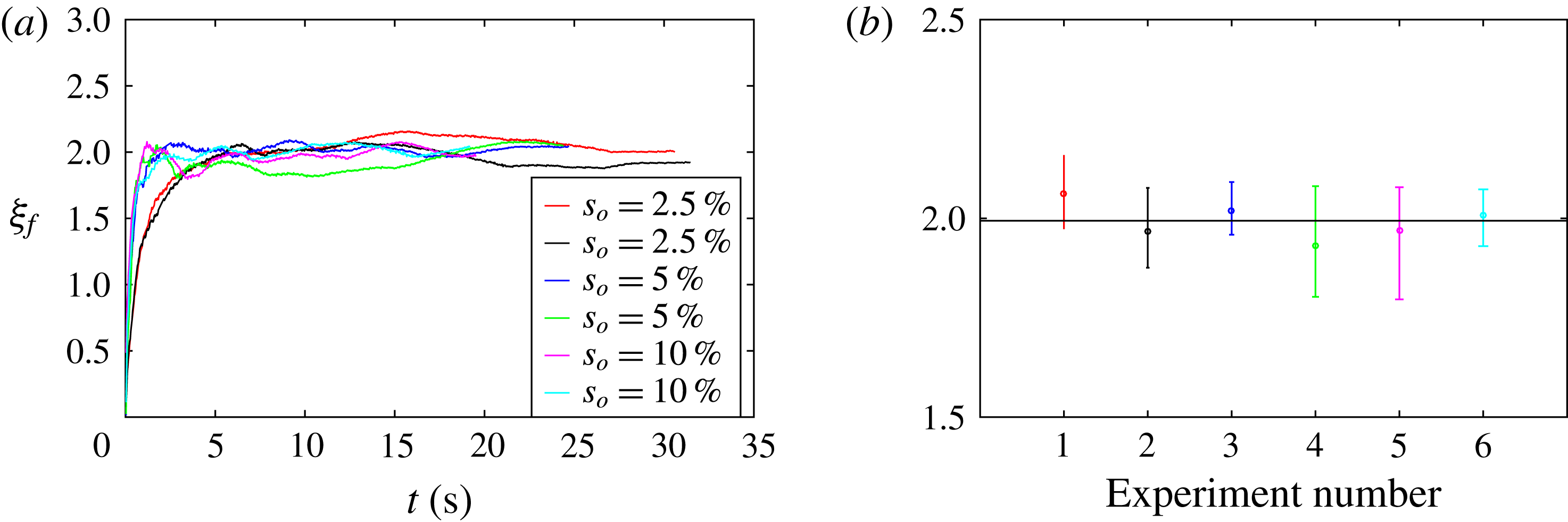
(a) Variation of the non-dimensional velocity
 $\unicode[STIX]{x1D709}_{f}$
with time for each of the six experiments. The legend shows the source salinity,
 $s_{o}$
, associated with each experiment. The average value of
 $\unicode[STIX]{x1D709}_{f}$
across each experiment and the corresponding error bars are represented in (b), retaining the same colour scheme as in (a), and the horizontal black line in (b) indicates the mean value of
 $\unicode[STIX]{x1D709}_{f}$
across the experiments.

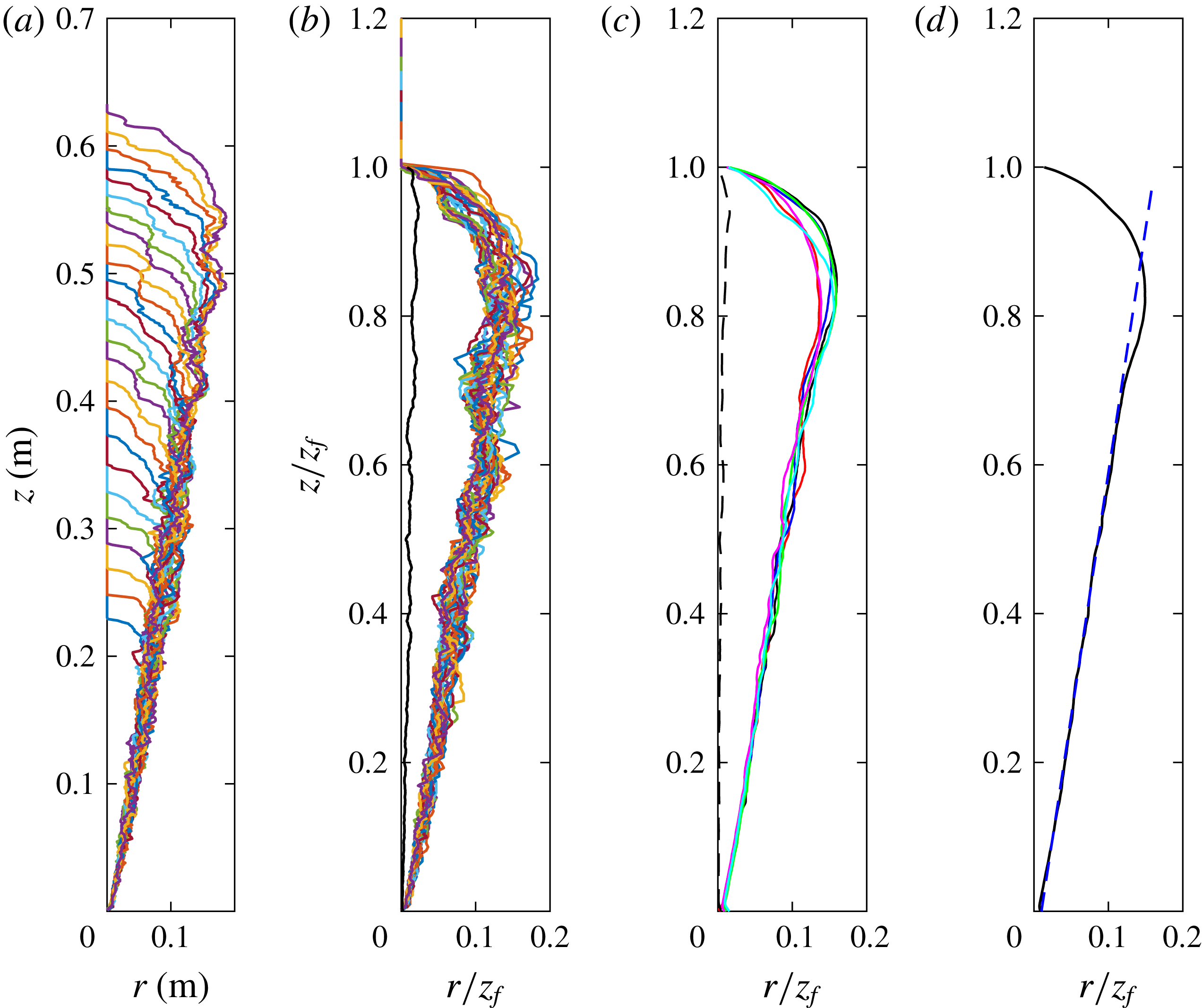
Variation of (a) the radius
 $r$
as a function of height
 $z$
, and (b) the rescaled radius
 $r/z_{f}$
as a function of rescaled height
 $z/z_{f}$
of the starting plume. Data are shown from 25 frames, recorded with a time interval of 1 s between frames. In (b), the black line represents the standard deviation of the rescaled data calculated for the experiment with
 $s_{o}=2.5\,\%$
and
 $Q_{o}=1.33~\text{cm}^{3}~\text{s}^{-1}$
. (c) Time average of the rescaled radius of the starting plume as a function of rescaled height for each of the six experiments, with the same colour scheme as in figure 1, with the black dashed line representing the standard deviation of the profiles relative to the mean. (d) Averaged shape of the starting plume obtained by averaging the profiles in (c). The blue dashed line represents the best fit for the radius of the steady plume which follows the plume head.

First a series of experiments were carried out in order to measure velocity of the front of the plume and the average shape of the plume head. We define the edge of the plume head as the point where the intensity of the dye, integrated through the plume, drops to 3 % of the maximum dye intensity at the source. For smaller values of dye intensity, the background noise becomes as significant as the signal. Using a larger threshold of 4 % leads to a reduction in the radius of the head by less than 8 %.
From dimensional analysis we expect that for a plume with a source buoyancy flux
 $\unicode[STIX]{x03C0}B_{o}$
, the velocity of the plume head will scale as
 $B_{o}^{1/3}z_{f}^{-1/3}$
, where
 $z_{f}$
is the position of the leading edge of the plume head,
 $$\begin{eqnarray}u_{f}=\unicode[STIX]{x1D709}_{f}{B_{o}}^{1/3}{z_{f}}^{-1/3}.\end{eqnarray}$$
Here
 $\unicode[STIX]{x1D709}_{f}$
may be taken to be the non-dimensional velocity obtained by integrating (2.1) with
 $u_{f}=\text{d}z_{f}/\text{d}t$
, and is given by
 $$\begin{eqnarray}\unicode[STIX]{x1D709}_{f}=\frac{z_{f}^{4/3}}{{\textstyle \frac{4}{3}}{B_{o}}^{1/3}(t+t_{o})}.\end{eqnarray}$$
The constant
 $t_{o}$
relates to the time taken by the plume to develop a plume head after issuing from the source. Figure 1(a) illustrates the variation of
 $\unicode[STIX]{x1D709}_{f}$
, using measured values of
 $z_{f}$
at each time
 $t$
, with different lines corresponding to different experiments. It is seen that the data collapse to a constant value after an initial adjustment above the source. The value of
 $t_{o}$
was estimated for each experiment to optimize the asymptote of
 $\unicode[STIX]{x1D709}_{f}$
to a constant value, and, in all cases, this has a value in the range 0.5–2.5 s, which is considerably shorter than the 20–30 s typical of the experiments.
Figure 1(b) shows the average value of
 $\unicode[STIX]{x1D709}_{f}$
for each experiment, with the colours corresponding to the legend in figure 1(a), and the error bars represent the variation of
 $\unicode[STIX]{x1D709}_{f}$
in each experiment after an initial adjustment time (see figure 1
a). The mean value of
 $\unicode[STIX]{x1D709}_{f}$
across experiments was found to be
 $1.99\pm 0.06$
.
The equations for the averaged top-hat velocity
 $u_{p}$
, radius
 $b$
, and reduced gravity
 $g_{p}^{\prime }$
for an established steady plume in an unstratified ambient are given by classical plume theory (Morton et al.
Reference Morton, Taylor and Turner1956),
 $$\begin{eqnarray}\frac{\text{d}u_{p}b^{2}}{\text{d}z}=2\unicode[STIX]{x1D6FC}u_{p}b,\quad \frac{\text{d}{u_{p}}^{2}b^{2}}{\text{d}z}=b^{2}{g_{p}^{\prime }}^{2},\quad \frac{\text{d}u_{p}b^{2}g_{p}^{\prime }}{\text{d}z}=0,\end{eqnarray}$$
where
 $\unicode[STIX]{x1D6FC}$
is the entrainment coefficient, which has a value of
 $0.13\pm 0.01$
(Morton et al.
Reference Morton, Taylor and Turner1956). Solving the steady-state plume equations given by (2.3) gives the average top-hat velocity within the plume
 $u_{p}$
as
 $$\begin{eqnarray}u_{p}=\frac{5}{6\unicode[STIX]{x1D6FC}}\left(\frac{9\unicode[STIX]{x1D6FC}B_{o}}{10}\right)^{1/3}z^{-1/3}=\unicode[STIX]{x1D709}_{p}{B_{o}}^{1/3}z^{-1/3}.\end{eqnarray}$$
Figure 2(a) illustrates the radius of the plume as a function of height in the plume at a series of times. By scaling the height
 $z_{f}$
and radius
 $r$
at a time
 $t$
by the position of the leading front of the plume
 $z_{f}(t)$
, we find that the starting plume can be mapped to a universal shape, suggesting that both the plume head and plume are self-similar, as shown in figure 2(b). In this figure, the black line represents the standard deviation of the plume radius for the 25 frames shown. The relatively large standard deviation is a result of turbulent fluctuations in the position of the edge of the plume with time. The plume profiles obtained in each experiment were time-averaged, and the mean profiles for the six experiments are shown in figure 2(c). In this figure, the black dashed line represents the standard deviation of these averaged experimental profiles. Figure 2(d) illustrates the average shape for the six experiments. The radius of the steady plume behind the plume head, shown in figure 2(d), increases linearly with height, as shown by the dashed line
 $r_{f}=\unicode[STIX]{x1D706}(z+z_{o})$
, where
 $\unicode[STIX]{x1D706}=0.15$
and
 $z_{o}$
is the virtual origin. The intercept on the line
 $r_{f}=0$
occurs at
 $z\approx -4.5\pm 1.5$
cm suggesting the virtual origin has value
 $z_{o}\approx 4.5$
cm, which is small compared to the distance of order 60–70 cm travelled by the plumes. The ratio of the velocity of the front of the plume head (2.1) to the velocity of a steady plume at that height (2.4) (
 $\unicode[STIX]{x1D709}_{f}/\unicode[STIX]{x1D709}_{p}$
) lies in the range
 $0.63\pm 0.04$
, which is consistent with the results of Turner (Reference Turner1962) (
 $0.61\pm 0.05$
) and Scase et al. (Reference Scase, Aspden and Caulfield2009) (0.65).
The linear increase in plume radius with height shown in figure 2(d) is observed to be valid only below the height
 $z=0.71z_{f}$
, after which the difference between the best-fit straight line modelling the radius
 $r_{f}$
and the average of the experimental data
 $r$
is observed to increase more rapidly (figure 2
d). We define this point to be the lower boundary of the plume head
 $z_{b}$
. By comparing the data with the model linear increase in radius with height, we find that in all experiments, the height of the lower boundary remains nearly constant,
 $z_{b}=(0.70\pm 0.02)z_{f}$
. Given the near constant ratio between
 $z_{b}$
and
 $z_{f}$
and the self-similar shape of the plume, we estimate the velocity of the lower boundary of the plume head
 $$\begin{eqnarray}u_{b}=\left(\frac{z_{b}}{z_{f}}\right)u_{f}=\unicode[STIX]{x1D709}_{b}{B_{o}}^{1/3}{z_{b}}^{-1/3}.\end{eqnarray}$$
The ratio of the velocity of the lower boundary of the plume head to the velocity of a steady plume at that height (
 $\unicode[STIX]{x1D709}_{b}/\unicode[STIX]{x1D709}_{p}$
) is found to be
 $0.39\pm 0.04$
. This is consistent with Turner’s (Reference Turner1962) estimate of 0.38 and the maximum theoretical prediction of 0.42 given by Delichatsios (Reference Delichatsios1979).
In order to help understand the interaction between the plume and plume head, pulses of dye were injected into the starting plume to enable the visualization of the path followed by individual fluid elements in the plume. The colour of the plume fluid was changed by injecting a small amount of dye (less than 0.2 cm
 $^{3}$
) through the nozzle using a syringe at a volume flux of
 $0.2~\text{cm}^{3}~\text{s}^{-1}$
, so that the volume flux of dye injected does not produce a significant change in the volume flux exiting the nozzle (which has value
 $Q_{o}=1.33~\text{cm}^{3}~\text{s}^{-1}$
). In experiment A, only one pulse of dye was injected at the time
 $t\approx 2.5$
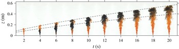
s to visualize the propagation of dye through the plume. Figure 3 illustrates the evolution of the pulse of dye in the plume. In this figure, the black dashed lines represent the positions of the front and back of the plume head as defined by the relation
 $z_{b}(t)=0.71z_{f}(t)$
. The series of photographs show, firstly, the accumulation of the pulse of dye within the region defined by
 $z_{b}<z<z_{f}$
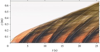
, and secondly, the irregular turbulent structure of the plume head as illustrated by the motion of the packets of dyed fluid which are visible approaching the leading edge of the plume. In experiment B, a pulse of dye was added to the source fluid at five successive times during the experiment in order to visualize the motion of the plume fluid as it rises towards the leading edge of the plume and then mixes into the plume head. In figure 4, we show a time series of a vertical line of pixels passing through the source. This figure illustrates the successive waves of dyed fluid which migrate to the front of the flow. Here they accumulate and mix into the head. In this figure two sets of lines are shown. First the two dashed lines follow the evolution of the front and back of the plume head. These lines are given by
 $$\begin{eqnarray}{z_{f}}^{4/3}={\textstyle \frac{4}{3}}\unicode[STIX]{x1D709}_{f}{B_{o}}^{1/3}(t+t_{o})\quad \text{and}\quad {z_{b}}^{4/3}={\textstyle \frac{4}{3}}\unicode[STIX]{x1D709}_{b}{B_{o}}^{1/3}(t+t_{o})\end{eqnarray}$$
consistent with (2.1) and (2.5). Secondly a series of dashed lines
 $z_{i}(t)$
are shown, each of which follows the ascent of one of the successive streaks of dye. These lines have the form
 $$\begin{eqnarray}{z_{i}}^{4/3}={\textstyle \frac{4}{3}}\unicode[STIX]{x1D709}_{s}{B_{o}}^{1/3}(t-t_{i}),\end{eqnarray}$$
where
 $t_{i}$
is the time of release of the
 $i$
th pulse of dye. Tracking the pulses of dye that reach the front of the plume gives an approximate estimate for
 $\unicode[STIX]{x1D709}_{s}$
, which has a value of approximately
 $3.82\pm 0.7$
. The error bar is found by using (2.7) to model the leading and trailing edge of each pulse of dye, which move at somewhat different speeds due in part to the effects of dispersion (cf. Rocco & Woods Reference Rocco and Woods2015). The estimate for
 $\unicode[STIX]{x1D709}_{s}$
is larger than the estimates of
 $\unicode[STIX]{x1D709}_{f}$
(1.99) and
 $\unicode[STIX]{x1D709}_{b}$
(1.25), and shows that the fluid in the steady plume which develops behind the plume head continually supplies fluid to the plume head, as is clear from the mean path followed by the dye.
Experiment A. Propagation of a pulse of dye through the plume and accumulation of dye in the plume head. The dashed lines indicate the positions of the front (
 $z_{f}$
) and back (
 $z_{b}$
) of the plume head, with
 $z_{b}=0.71z_{f}$
. In this experiment,
 $s_{o}=5\,\%$
,
 $Q_{o}=1.33~\text{cm}^{3}~\text{s}^{-1}$
. The time interval between frames is 2 s.

Experiment B. Time series of the vertical centreline of the plume. The dashed lines show the
 $t^{3/4}$
characteristics for the position of the front (black) and back (yellow) of the head, and of the pulses of dye (white). In this experiment, the initial salinity,
 $s_{o}=5\,\%$
, and the volume flux at the source,
 $Q_{o}=1.33~\text{cm}^{3}~\text{s}^{-1}$
.

3 Modelling the plume head
We now build a model of the mass, momentum and buoyancy conservation in the plume head in order to estimate the mixing of ambient fluid directly into the head, and also to test the momentum balance of the head. The model describes an ensemble average of the flow averaged over several realizations of the flow so that fluctuations associated with the detailed distribution of individual eddies in the flow are averaged. The plume behind the plume head is modelled as being steady, while the plume head slowly evolves in time and space. We define the plume head to correspond to the region
 $z_{b}<z<z_{f}$
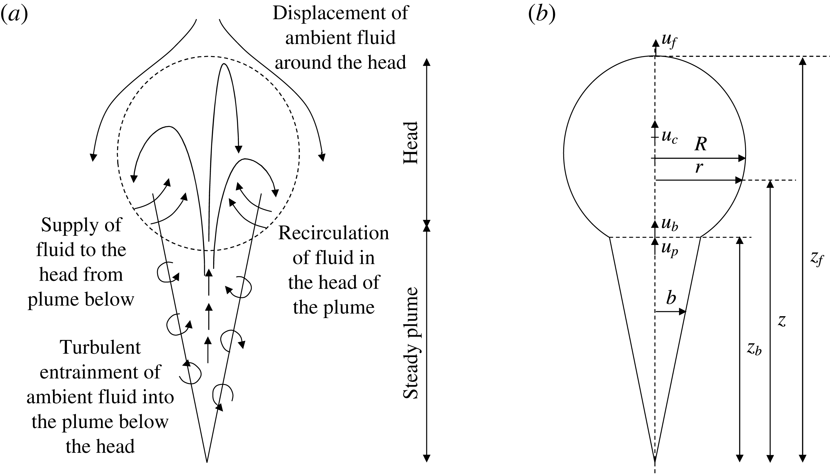
as defined by figure 2(d). Figure 5(a) captures the observations from figures 3 and 4 in a schematic, and figure 5(b) illustrates the shape of the starting plume and the various parameters involved in the modelling of the plume head.
(a) Cartoon illustrating the motion of fluid within the starting plume and the motion of ambient fluid around the plume head. The motion of fluid within the plume head shown is in the frame of reference of the plume head. (b) Illustrating various dimensions and velocities.

3.1 Conservation of volume
The volume of the plume head
 $V_{c}$
is found by evaluating the integral
 $$\begin{eqnarray}V_{c}=\int _{z_{b}}^{z_{f}}\unicode[STIX]{x03C0}r^{2}\,\text{d}z,\end{eqnarray}$$
where
 $r=r(z)$
is the radius of the starting plume as given by the shape profiles shown in figure 2(a–d). Similarly, the vertical momentum of the plume head is defined as
 $$\begin{eqnarray}M_{c}=\int _{z_{b}}^{z_{f}}\unicode[STIX]{x03C0}r^{2}u\,\text{d}z,\end{eqnarray}$$
where
 $u$
, the horizontally averaged vertical velocity at height
 $z$
in the plume head, is given by
 $u=u_{f}(z/z_{f})$
in order that the shape of the plume head remains similar at all times. The velocity of the centre of mass of the plume head
 $u_{c}=\text{d}z_{c}/\text{d}t$
is found by combining (3.2) with (3.1) (
 $u_{c}=M_{c}/V_{c}$
). The estimate for the position of the centre of mass of the plume head,
 $z_{c}$
, was found to have a near constant value over all the experiments,
 $z_{c}=(0.83\pm 0.01)z_{f}$
. We can define a shape factor
 $\unicode[STIX]{x1D6FA}$
for the plume head as
 $$\begin{eqnarray}\unicode[STIX]{x1D6FA}=\frac{V_{c}}{(z_{c}-z_{b})R^{2}},\end{eqnarray}$$
where
 $R$
is the maximum radius of the plume head (see figure 5
b). The average shape factor for the plume head was found to be 5.41, which is a larger value than the shape factor of an equivalent ellipsoid (
 $=4\unicode[STIX]{x03C0}/3\approx 4.19$
). Therefore the volume of the plume head as defined in (3.1), and using the 3 % dye threshold, which is the limit of our experimental method, was found to be approximately 23 % larger than the volume estimates of Turner (Reference Turner1962) and Scase et al. (Reference Scase, Aspden and Caulfield2009), where the plume head was assumed to have a spherical shape.
The plume head is supplied with fluid by the steady plume. The volume flux of fluid supplied by the steady plume to the plume head can be found by solving the steady plume equations for the radius and the velocity as defined earlier (Morton et al.
Reference Morton, Taylor and Turner1956). The flux entering the plume head, evaluated at
 $z=z_{b}$
, is given by
 $Q_{p}=\unicode[STIX]{x03C0}b^{2}(u_{p}-u_{b})|_{z=z_{b}}$
, where the expression
 $(u_{p}-u_{b})$
accounts for the fact that the plume head is advancing. The equation for conservation of volume of the plume head is given by
 $$\begin{eqnarray}\frac{\text{d}V_{c}}{\text{d}t}=Q_{p}+\unicode[STIX]{x1D716}{V_{c}}^{2/3}u_{c},\end{eqnarray}$$
where the second term on the right hand side gives the flux due to entrainment of ambient fluid into the plume head. Solving (3.4) using the estimates of
 $V_{c}$
,
 $Q_{p}$
,
 $u_{c}$
and
 $z_{b}$
, suggests that the ratio
 $Q_{p}/(\text{d}V_{c}/\text{d}t)=0.88\pm 0.06$
. This implies that the time-averaged volume flux entrained directly into the plume head is small compared to the flux supplied from the steady plume. The range of values of
 $Q_{p}/(\text{d}V_{c}/\text{d}t)$
is consistent with the error in our measurement of
 $\text{d}V_{c}/\text{d}t$
, and arises in part owing to the turbulent fluctuations of the flow and in part owing to the uncertainty in the precise value of the entrainment coefficient of the steady plume,
 $\unicode[STIX]{x1D6FC}$
. Based on our data, we estimate that
 $\unicode[STIX]{x1D716}=0.14\pm 0.08$
. If the plume head were to entrain over its entire surface area (
 $S_{c}=\int _{z_{b}}^{z_{f}}2\unicode[STIX]{x03C0}r\,\text{d}z$
), then the equivalent entrainment coefficient per unit surface area would be
 $0.04\pm 0.02$
, which is smaller than for a steady plume, and consistent with the entrainment coefficient for the plume head, 0.04–0.05, as proposed by Scase et al. (Reference Scase, Aspden and Caulfield2009).
3.2 Conservation of buoyancy
The conservation of buoyancy for the plume head is given in terms of the flux of buoyancy entering the head from the steady plume. Since the flux of buoyancy is defined as
 $\unicode[STIX]{x03C0}g_{p}^{\prime }b^{2}u_{p}$
in the top-hat model, then since the rear of the plume head advances with speed
 $u_{b}$
, the flux entering the plume head is given by
 $\unicode[STIX]{x03C0}b^{2}(u_{p}-u_{b})g_{p}^{\prime }=Q_{p}g_{p}^{\prime }$
. This leads to the equation for the conservation of buoyancy,
 $$\begin{eqnarray}\frac{\text{d}g_{c}^{\prime }V_{c}}{\text{d}t}={Q_{p}g_{p}^{\prime }|}_{z=z_{b}}.\end{eqnarray}$$
Here
 $g_{c}^{\prime }$
is the reduced gravity of the plume head averaged throughout the plume head, and
 $g_{p}^{\prime }$
is the reduced gravity of the following steady plume, averaged across a horizontal surface at height
 $z$
, obtained by solving the steady-state plume equations (Morton et al.
Reference Morton, Taylor and Turner1956)
 $$\begin{eqnarray}g_{p}^{\prime }(z)=\frac{5B_{o}}{6\unicode[STIX]{x1D6FC}}\left(\frac{9\unicode[STIX]{x1D6FC}B_{o}}{10}\right)^{-1/3}(z+z_{o})^{-5/3},\end{eqnarray}$$
where
 $z_{o}$
is the virtual origin of the plume. The total buoyancy in a steady plume in the region
 $0<z<z_{b}(t)$
is given by
 $$\begin{eqnarray}\unicode[STIX]{x03C0}\int _{0}^{z_{b}}g_{p}^{\prime }(z)b(z)^{2}\,\text{d}z=\left(\frac{3\unicode[STIX]{x03C0}}{4}\right)\left(\frac{6\unicode[STIX]{x1D6FC}}{5}\right)\left(\frac{9\unicode[STIX]{x1D6FC}}{10}\right)^{-1/3}{B_{o}}^{2/3}[(z_{b}+z_{o})^{4/3}-{z_{o}}^{4/3}].\end{eqnarray}$$
In the limit
 $z_{o}\ll z_{b}$
, appropriate for our experiments with
 $z_{o}\sim 4.5$
cm and
 $z_{b}\sim 60{-}70$
cm, we may approximate the right-hand side of (3.7) by the expression
 $$\begin{eqnarray}\left(\frac{3\unicode[STIX]{x03C0}}{4}\right)\left(\frac{6\unicode[STIX]{x1D6FC}}{5}\right)\left(\frac{9\unicode[STIX]{x1D6FC}}{10}\right)^{-1/3}{B_{o}}^{2/3}{z_{b}}^{4/3}=\left(\frac{\unicode[STIX]{x1D709}_{b}}{\unicode[STIX]{x1D709}_{p}}\right)\unicode[STIX]{x03C0}B_{o}t,\end{eqnarray}$$
where
 $\unicode[STIX]{x03C0}B_{o}t$
is the total buoyancy supplied from the source up to a time
 $t$
, and
 $\unicode[STIX]{x1D709}_{p}$
and
 $\unicode[STIX]{x1D709}_{b}$
are defined in (2.4) and (2.6), respectively. Here
 $(\unicode[STIX]{x1D709}_{b}/\unicode[STIX]{x1D709}_{p})=0.39\pm 0.04$
(see § 2). The remainder of the buoyancy accumulates in the plume head and is given by
 $$\begin{eqnarray}\left(1-\frac{\unicode[STIX]{x1D709}_{b}}{\unicode[STIX]{x1D709}_{p}}\right)\unicode[STIX]{x03C0}B_{o}t=(0.61\pm 0.04)\unicode[STIX]{x03C0}B_{o}t.\end{eqnarray}$$
3.3 Conservation of momentum
We propose that the equation for conservation of momentum of the plume head has the form
 $$\begin{eqnarray}(1+A)\frac{\text{d}M_{c}}{\text{d}t}={Q_{p}u_{p}|}_{z=z_{b}}+g_{c}^{\prime }V_{c}-C_{d}u_{c}^{2}(\unicode[STIX]{x03C0}R^{2}),\end{eqnarray}$$
where
 $A$
is the added mass of the plume head, and the first two terms on the right hand side denote the momentum flux supplied to the plume head by the fluid entering from the following steady plume and the buoyancy force on the head. We have also included a drag force, with drag coefficient
 $C_{d}$
, which is similar in effect to form drag on a moving body. The added mass,
 $A$
, arises due to the acceleration of ambient fluid around the head, thus contributing an increased force on the plume head (Ohl, Tijink & Prosperetti Reference Ohl, Tijink and Prosperetti2003).
We note that this model differs from some of the earlier literature in which the plume head has been modelled as a spherical vortex (Turner Reference Turner1962; Scase et al. Reference Scase, Aspden and Caulfield2009). Our observations of the structure and motion of fluid in the plume head (figures 3 and 4) suggest that the flow does not develop a coherent vortex-ring-type structure. We observe a more irregular motion as turbulent pulses of buoyant fluid supplied to the plume head reach the plume front and spread radially, with successive parcels spreading in different directions. Instead, our approach follows from the work of Scorer (Reference Scorer1997) who proposed a similar momentum conservation equation for a discrete thermal, although he did not include the turbulent drag term since he did not measure the shape of the thermal independently of the momentum equation.
We have solved (3.4) and (3.5) with the modified momentum equation for the plume head given by (3.10) to find the drag coefficient
 $C_{d}$
, which has a value
 $4.2\pm 1.4$
. The range of values of
 $C_{d}$
correspond to the uncertainty in our estimate of
 $\unicode[STIX]{x1D716}$
, and hence we establish a relationship between the entrainment coefficient
 $\unicode[STIX]{x1D716}$
and drag coefficient
 $C_{d}$
of the plume head by combining (3.4) and (3.10),
 $$\begin{eqnarray}C_{d}=(6.0\pm 0.3)-(11.8\pm 1.2)\unicode[STIX]{x1D716}.\end{eqnarray}$$
The added mass of the plume head was assumed to be equal to the added mass of a sphere,
 $A=0.5$
, consistent with Scorer (Reference Scorer1997) and Ohl et al. (Reference Ohl, Tijink and Prosperetti2003).
4 The starting plume in a stratified ambient
In this section, we describe how a starting plume rises through a linearly stratified ambient, characterized by the buoyancy frequency
 $N$
, where
 $N^{2}=-(g/\unicode[STIX]{x1D70C}_{o})(\text{d}\unicode[STIX]{x1D70C}_{a}/\text{d}z)$
, in which
 $\unicode[STIX]{x1D70C}_{a}$
is the density of the ambient at height
 $z$
and
 $\unicode[STIX]{x1D70C}_{o}$
is a reference density.
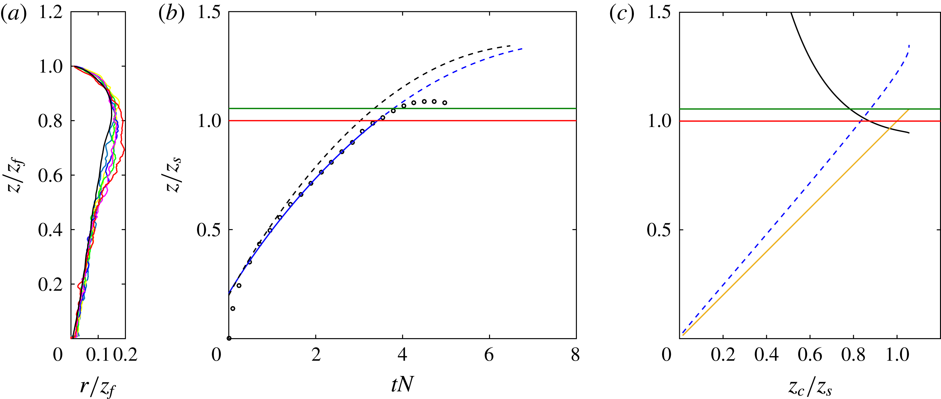
(a) Rescaled radius
 $r/z_{f}$
as a function of the rescaled height
 $z/z_{f}$
in a linearly stratified ambient. The figure shows the radius averaged across five experiments when the plume is at different fractions of the maximum top height
 $z_{T}$
(
 $z_{f}/z_{T}=0.5{-}1.0$
). The red profile shows the profile of radius when the plume reaches its top height (
 $z=z_{T}$
). The black profile shows the equivalent profile in an unstratified ambient (see figure 2
d). In the five experiments,
 $N^{2}=0.35$
,
 $Q=1.01~\text{cm}^{3}~\text{s}^{-1}$
,
 $s_{o}=10\,\%$
, 12 %, 13 %, 14 %, 15 %. (b) Plot of dimensionless height of rise (
 $z/z_{s}$
) versus time (
 $tN$
), where
 $z_{s}$
is the maximum height of the steady plume in a stratified ambient. The graph illustrates the height of rise as predicted by the new model (blue), and is compared against experimental data (black circles) and the model proposed by Turner (Reference Turner1962) using the equivalent top-hat coefficients estimated by Scase et al. (Reference Scase, Aspden and Caulfield2009) (black). In (c), the instantaneous neutral height of the plume head (black), which is the height in the ambient at which the density of the plume head equals the density of the ambient, and the positions of the centre (yellow) and top (blue) of the plume head are shown. The horizontal lines in (b) and (c) show the maximum height of the continuing steady plume (red) and the maximum height of rise of the centre of the plume head (green) as predicted by the model.

We have carried out a series of experiments in which we set up a linear stratification in the experimental tank with
 $N^{2}=0.35~\text{s}^{-2}$
. We then explored the ascent of series of starting plumes with volume flux
 $Q_{o}=1.01~\text{cm}^{3}~\text{s}^{-1}$
and salinity
 $s_{o}=10$
, 12, 13, 14, 15 %. In figure 6(a) we illustrate the variation of the rescaled radius (
 $r/z_{f}$
) as a function of the rescaled height (
 $z/z_{f}$
) at the different times when the plume height
 $z_{f}$
was a fraction 0.5 (grey), 0.6 (yellow), 0.7 (blue), 0.8 (green), 0.9 (purple), and 1.0 (red) of the maximum height of rise of the starting plume
 $z_{T}$
. In each case, we have averaged the profile over the five experiments. The figure shows that as the plume approaches the maximum height, the plume radius begins to increase as it slows down and intrudes laterally. For reference, the black profile represents the equivalent profile of the plume in an unstratified environment (figure 2). In figure 6(b), we illustrate the average of the experimental data for the height of the top of the plume head as a function of dimensionless time,
 $tN$
(black circles).
To include stratification in the model of a starting plume, we modify the buoyancy conservation equation (3.5) to the form (cf. Morton et al. Reference Morton, Taylor and Turner1956)
 $$\begin{eqnarray}\frac{\text{d}g_{c}^{\prime }V_{c}}{\text{d}t}=Q_{p}{g_{p}^{\prime }|}_{z=z_{b}}-N^{2}V_{c}u_{c}.\end{eqnarray}$$
We now solve (3.4), (3.10), and (4.1), for mass, momentum, and buoyancy conservation of the plume head, coupled with the solutions of the steady plume equations in a stratified environment (cf. Morton et al.
Reference Morton, Taylor and Turner1956) to calculate the supply of volume, momentum, and buoyancy into the plume head. To complete the model, we need to specify the shape of the plume head in order to relate the position of the base of the head,
 $z_{b}$
, to the position of the centre of mass of the head,
 $z_{c}$
, and to estimate the radius of the head,
 $R$
, according to (3.3).
Below the maximum height of rise, before the shape of the plume is influenced by the stratification (figure 6
a), we might expect that the relationships between
 $z_{b}$
,
 $z_{c}$
,
 $z_{f}$
, and
 $\unicode[STIX]{x1D6FA}$
for the unstratified case (
 $z_{b}/z_{f}=0.71$
,
 $z_{c}/z_{f}=0.83$
,
 $\unicode[STIX]{x1D6FA}=5.41$
) provide a reasonable approximation. In these calculations, we also need a specific value of the drag coefficient,
 $C_{d}$
, and the entrainment coefficient,
 $\unicode[STIX]{x1D716}$
, which were only constrained by the relation
 $C_{d}=(6.0\pm 0.3)-(11.8\pm 1.2)\unicode[STIX]{x1D716}$
from our experiments in an unstratified ambient. We find that the error between the model and experimental data is less than 5 % for the range of values of
 $C_{d}$
given by the relation (3.11). The predictions of the model are shown in figure 6(b) (blue line), where the mean value of
 $\unicode[STIX]{x1D716}(=0.14)$
was used to constrain the value of the drag coefficient
 $C_{d}$
. Figure 6(b) also shows the predictions using the vortex-ring model proposed by Turner (Reference Turner1962) and Scase et al. (Reference Scase, Aspden and Caulfield2009) (black dashed line), in which the parameters were taken from those given by Scase et al. (Reference Scase, Aspden and Caulfield2009). We used the parameters from Scase et al. (Reference Scase, Aspden and Caulfield2009), since in the original work of Turner (Reference Turner1962), the speed of the back of the plume head was assumed to equal a fraction 0.6 of the maximum centreline speed of the steady plume rather than a fraction 0.6 of the top-hat speed as used by Scase et al. (Reference Scase, Aspden and Caulfield2009), and which is consistent with our experimental results. Equation (4.1) was used to describe the conservation of buoyancy. The figure shows that the new model predicts the height of rise somewhat more accurately until the plume reaches the maximum height of the steady plume, where the shape of the plume head and its dynamics change as a result of the stratification (figure 6
a). Figure 6(c) illustrates the variation of the height at which the plume head would be neutrally buoyant (black line) as a function of the height of the centre of the plume head, as well as the height of the top (blue dashed line) and centre (yellow line) of the plume head. The neutral buoyancy height of the plume head, which occurs where the yellow and black lines meet, is very similar to the maximum height of the steady plume (red horizontal line). The maximum overshoot of the centre of the plume head above this height (green horizontal line), as predicted by the model, is comparable to the experimental measurement of the maximum height of rise of the plume head as shown in figure 6(b). However, given the distortion of the shape of the plume head near the maximum height of rise (figure 6
a), we do not expect the model prediction for the height of the leading edge of the plume head to follow accurately the motion of the leading front of the plume head beyond this height.
5 Discussion
In this paper we have carried out some new experiments to describe the mixing and interaction between the plume head, the following steady plume, and the ambient. We found that the buoyancy force on the plume head combined with the momentum flux supplied to the plume head from the following steady plume exceed the rate of change of momentum of the plume head. We propose that a turbulent drag on the plume head develops which accounts for this difference. We have estimated that the drag coefficient is given by
 $C_{d}=4.2\pm 1.4$
, with the range of values corresponding to the uncertainty in the estimate of the entrainment coefficient
 $\unicode[STIX]{x1D716}=0.14\pm 0.08$
. The range of values of the entrainment coefficient suggest that the plume head entrains only a small fraction of its volume from the ambient, with the dominant influx of fluid supplied by the following steady plume. We also found that a fraction
 $0.61\pm 0.04$
of the total buoyancy supplied by the source lies within the plume head, so that the plume head is more buoyant than the developing steady plume immediately behind at
 $z=z_{b}$
.
In a stratified ambient the assumption that the plume head retains the same shape as in the unstratified case allows an initial estimate for the height of rise with time, which compares well with experimental data up to the point at which the plume head reaches the maximum height of rise of the ensuing steady plume. It would be of interest to explore the evolution of the plume head beyond the maximum height, perhaps with an investigation into the dynamics of a negatively buoyant forced thermal in a uniform and stratified environment, to understand the dynamics and the deformation of the plume head near its maximum height.
When a steady flux of buoyancy, generating a steady turbulent plume, is suddenly increased to a substantially larger value, then a mixed zone of fluid may develop and grow in the transition region, somewhat akin to the starting plume. It would be of interest to develop the experimental modelling presented herein to estimate the drag and entrainment coefficients associated with such transition zones in order to build a model of their evolution.