The Chair (Mr S. M. Shepley, F.I.A.): It gives me pleasure to chair a session on a general insurance topic which is at the forefront of how actuaries can create value for insurance companies.

The paper is a technical one on general insurance pricing: ‘case deleted’ deviance. The paper covers practical applications and mentions some of the important issues of today around personal injury and bodily injury.

Let me introduce the authors before they introduce the paper.

Mr Anthony Lovick graduated in mathematics from Oxford University in 1987 and qualified as a Fellow of the Institute of Actuaries in 1994. He spent 21 years with the Aviva Group, before joining EMB as a senior consultant. He undertook a number of roles with Aviva, most recently as Price Optimisation Actuary, and focused on Pay As You Drive. He was also head of statistics and development in the personal lines business. As the actuary leading the research for Pay As You Drive, he helped inspire the analysis, build the data warehouse systems and launch of the product to market. As part of this project, Aviva prepared two patents with Mr A C Lovick listed as the inventor, one of which is now granted.

Mr Peter Lee is a Director at EMB Towers Watson and global lead in pricing innovation with over 20 years’ experience in non-life insurance. Prior to joining EMB, he worked at Allianz UK as the Personal Lines Actuary. At EMB, Mr Lee worked for a large number of insurers throughout the world in different regulatory regimes, advising over a broad spectrum of areas and products ranging from claims reserving to pricing and the design of management information. Throughout his career he has been at the forefront of innovation, being one of the pioneers of the application of statistical modelling to personal lines pricing and then extending these techniques to commercial lines. More recently, Mr Lee developed EMB's price optimisation solution which has now been implemented in many of the largest general insurers across the world. Much of his work involves embedding technical analysis and demand-based pricing into a wider pricing process, allowing these enhanced capabilities to be more effectively leveraged. Mr Lee is now working with clients to link pricing and marketing to provide an enhanced framework for managing customer value.

Mr P. K. W. Lee, F.I.A. (introducing the paper): Our paper focuses on trying to build models that are most predictive going forward, which are not necessarily models that best fit the historic data.

The concepts behind the paper, which cover why we came up with this methodology which we call the ‘case deleted’ deviance, are best covered by a very basic example. We came up with this methodology to address what people call ‘Winner's Curse’ and the advent of the price comparison sites.

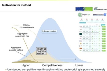
Many will have seen a diagram like Figure 1. It demonstrates that it is in the aggregate channel that the business you write tends to be the most competitive business. In other words, any errors in your model are punished severely compared to a normal direct internet channel or a direct phone channel. The fundamental reason why we came up with this methodology is to try to improve the predictive capability of risk premium models.

Figure 1

The Winners Curse

The problem with the models we build currently comes down to the nature of the data we have in insurance applications: ‘sparse data’. ‘Sparse data’ is when there is lots of exposure – often, for example, millions of records in a personal line – and not many claims. So, the claim frequency in most lines of business is very low. This sparse data throws up certain challenges.

As practitioners we are familiar with generalised linear modelling (GLM). A newer problem, which has been thrown up by the price comparison sites, is the level of extrapolation to apply in our GLM models. The price transparency and the range of quotations in price comparison sites leads to wider quote profiles.

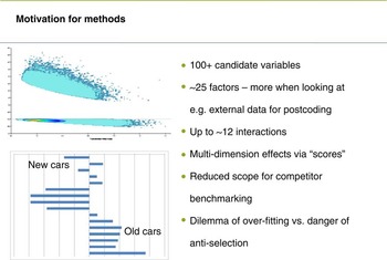
The chart on the left of Figure 2 shows the difference between a new business profile and a renewal profile for an insurance company. The new business profile is much more weighted towards older vehicles and the model is based on historic experience which would be an older profile. The models are being extrapolated much more in a price comparison environment.

Figure 2

The dilemma of overfitting or anti-selection

The insurers’ reaction to this includes narrowing the underwriting footprint and increasing the number of rating factors used in the rating structure. It is not uncommon, particularly if looking at postcode allocation, to have hundreds of candidate variables. There can be up to 25 variables and dozens of interactions.

I contend that this is moving into over-fitting territory in terms of these models. It is not straightforward to find out where there is over-fitting. We look at each candidate selected variable, the time test, and the statistical test, and applied common sense to include all the factors, because we have gone through quite a vigorous modelling process. But if all 20 variables are included in the whole, there is probably over-fitting.

So, we decided not to have a binary decision of whether to exclude or include a factor. We decided to scale back the relativities instead of making a binary decision.

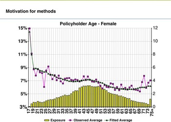
Any modelling process tries to extract a signal from the noise. Consider a basic example of female age curves as set out in Figure 3. We fitted a curve and removed the noise.

Figure 3

A Spline fit of Policyholder Age

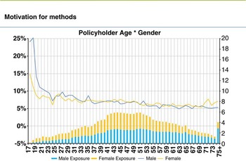
A more topical example is age and gender as set out in Figure 4.

Figure 4

The Gender vs Age interaction

This is a quite good illustration of a GLM's power. This shows that where there is apparently little exposure at the young end, there is a clear signal coming out that females are much better than the males at a very young age, which is a well-known fact. Despite the very low exposures, the GLM's are still picking up quite a strong signal. That is why we do not favour the binary approach. Clearly, what is uncertain given the low exposure is the absolute relativities.

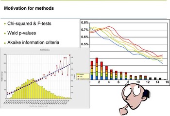
When we build a model there are lots of tools in our armoury as shown in Figure 5: lots of statistical tests, and also Akaike information criteria, which tries to penalise the number of parameters used. There are variations of the tests, for example, the Bayesian version.

Figure 5

Time dependency and Stats tests

In practice a lot of these tests find things that are significant. Interactions in most circumstances tend to be significant in purely statistical tests but, as a practitioner, it is difficult to justify them. There are other tests that can be applied to balance that. One would be the time test. You can see an example on the graph in Figure 5 which shows a vehicle age and theft frequency chart over time. As car security has improved, the shape of the vehicle age to theft frequency relativities have changed. Having a time test often is not great because you can have a genuine time trend.

Another tool in the armoury is ourselves. We, as actuaries, add some value and apply common sense. Obviously, we are working with our underwriters. No model is built purely automatically.

Increasingly common is also what is called a ‘hold out’ test. So, for example, you might build your model with 80% of the data and you hold back 20% and test that model against the 20% hold out. There are lots of tools in our armoury but we feel that there is still a need for a more robust test. One example in the paper, shown in figure 1 of the paper, is that we randomly generated a variable, and this passed the statistical test. If you applied 5% significance that would probably happen one-in-20 times anyway.

Another example, figure 11 in the paper, from a paper that Mr John Berry did as part of GIRO, is looking at what he called the Gini coefficient and U–statistic that looks at how all models degrade over time. These are conversion models. They are built on three months’ data and you can see instantly that the models start to degrade immediately, so that the higher the number, the better the fit. That indicates that you are probably overfitting to the history. We will demonstrate how we resolve some of those issues today.

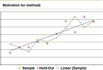
To illustrate the general approach adopted at a simple level, consider Figure 6.

Figure 6

The hold-out sample

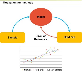
A straight line is fitted to the sample data points, which often happens in practice today, the sample typically might be 80% of the data. You estimate some parameters and then you test against a hold out sample. The issue is whether or not the fit is good to the hold out sample. If that fit is not good, how do you resolve that without actually using the hold out sample? So you can end up going around in circles, see figure 7.

Figure 7

Adjusting parameters – the circular reference

Do you resample it? Do you actually include it back into the data? Mr Lovick will describe how we resolved that circular reference issue.

Now, let me turn to what we mean by ‘case deleted’ deviance. A standard deviance is simply the sum of squared errors in the normal distribution linear regression case. It can be pictured, as depicted in Figure 8, as the distance between the data point and the fitted value (y_i and μ_i in the diagram).

The concept of case deleted is that we are going to delete the data point, and the fitted value would move away from the data point. We then use the sum squared of the distance between the adjusted fitted value with the data point (y_i, μ_(i)) as the contribution of that data point to the deviance. So that requires us to fit n models, where n is the number of data points. If there are 10 million observations that requires a fit of 10 million models in theory, which is impractical. There are some approximations that can be applied which takes us to ‘case deleted’ deviance. Instead of using the actual fitted value of that data point in the model, it deletes that data point and then it is the distance between that data point and the adjusted fitted value. Every single data point is summed in that manner to get a new deviance function, to give what we call a case deleted deviance.

The difference between case deleted deviance can be viewed as a pattern. If you delete that data point that is akin to removing the noise of that data point. We have defined this new term as the value measure, which is the pattern less five times the value. The correlation of the value with standard errors is shown in figure 3 of our paper.

We tested the value on a small number of datasets. We scaled so that where the value is positive, the increase of value is positive. It means that that parameter adds value. If it is negative, it reduces value. From this process we got the five to be used in the value. There is more work to do with more datasets to confirm that five should be the number.

To fit the values we draw upon a number of approximations. To work out case deviance for, say, 10 million observations is impractical as it requires us to fit 10 million models. From one model fit we have approximated adjusted fitted values for each data point.

The graphs in figures 8 and 9 of our paper show case deleted estimate approximations for Log-Poisson and Logit-Binomial. The x-axis is the difference in fitted values of the approximation divided by the difference in the fitted values of the accurate method.

Figure 8

Standard and “Case Delete” Estimates

Figure 9

Vehicle Group Spline

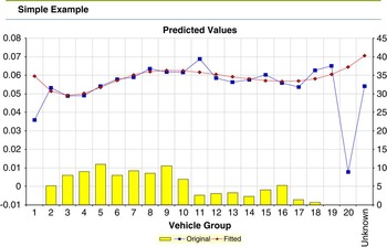
Our research includes an example of fitting a semi-realistic accidental damage data frequency model. It was Log-Poisson with about 100- parameters. We deleted or removed each point in turn and then calculated the value function as shown in Figure 9.

Each point here represents a parameter. We also plotted that against the standard error of percentage used in normal GLM models.

Our normal cut-off point is 50%, which is broadly similar to the positive value and broadly equivalent to the standard methodology. However it does throw up some interesting outliers which merit further investigation. We progressed through with a further simple example based on the vehicle group as depicted in Figure 10.

Figure 10

Varying the number and position of knots in the spline

We tested the value function for the random variable that we had in our paper. The value function rejected the random factor, which was a step forward. We fitted a cubic spline to the vehicle group. and explored the different knot positions. By moving the cubic spline to different positions we plotted the value. This indicated the cubic spline, probably number six, is the maximum value, that is to say that the knot position should be position six.

The lines show that once the knot position is fixed at six, a second knot should be added. However adding additional knots does not broadly add any value because the value is much less. It is probably better to use this value measure to come up with a more robust sort of stepwise regression algorithm example.

Mr A. C. Lovick, F.I.A. (also introducing the paper): To summarise, we have a case deleted deviance, having started with the 80:20 hold-out sample concept, and generated from that the logical extension of doing an n-fold hold-out, where you hold-out one row at a time, and doing that 10 million times through the dataset.

We got round the practical problem of fitting the model 10 million times by producing a fast approximation that is 99.9% accurate. That means that you can fit your model once and then run this calculation across the dataset once to get all of those answers for the case deleted deviance.

We have come up with a parameter of five which seems to distinguish adding value from declining value when you have changed the model in some way. By calibrating it to be positive or negative, that means that that value seems to be a useful absolute number in its own right.

There remains the problem of how to get round the circular reference that Mr Lee spoke about. That is needed because the case deleted deviance is restricted to helping test, with a number, whether the change made to the model is useful or not. It has not solved the problem of when parameters are added to the model of making a binary decision about whether it is in or out. We searched for a mechanism that would allow us to scale those parameters in a kind of Bayesian credibility way, which might lead to conclude: “here is a percentage that you should include or exclude that parameter, somewhere between nought and 100%, or possibly even slightly higher than 100%”.

This brings us to the noise reduction method or technique to achieve this, which may not be entirely obvious from the paper. The case deleted deviance can increase if you add noise to your model.

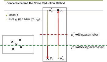
On the left-hand side of Figure 11, there could be millions of data points, which may be very firm leading to a stable estimate for the model. However, there could be a sparse corner on the right-hand side, and in that box there are only two data points. If there are no parameters which apply specifically to the data points in that box, then the estimate from these 10 million points will produce the green line – that will be the estimate that will be applied to the two data points in this box.

Figure 11

“Case Deleted Deviance” increasing with model complexity

As Mr Lee said, we can think of this specifically in the normal distribution identity link function method as exactly equivalent to calculating a sum of squares. So for these two data points, the deviance will be the sum of squares of the distances of the two red lines in Figure 11.

Now, if a new parameter is added to the subset of data in the right box, we get model 2 in Figure 12 where μ_i will float to the mean of the data in scope, giving distances, which, on a sum of squares basis, you can understand that these are smaller than the previous.

Figure 12

“Case Deleted Deviance” increasing with model complexity

If you then work out what the case deleted deviance means in this circumstance you find that the case deleted equivalents are the same distances, SD(y_i, μ_i) is equal to CDD(y_i, μ_i). You can see this by if you drop out y₁, and you re-fit the model. Then instead of floating to the middle, the parameter cannot float to there because it now cannot take account of this data point, so instead the parameter will take the estimate all the way up to the top. Exactly the opposite is true if you delete this point y₂. Then the estimate for y₂ will come all the way down to be equal to y₁.

Adding a parameter to that data point box there, clearly adds noise. The sum of squares difference that you get from that is much bigger than with the parameter in the model but it is also bigger than when the parameter was not in the model. So therefore the case deleted deviance has actually increased when you added this parameter. So it is revealing quite clearly that if you add too much noise to the model, this measure is useful because it will say, “This is all rubbish, you just added lots of noise. You need to take some back out again.”

So, the question is how do we then apply that to use that mechanism to scale all of the parameters in our model?

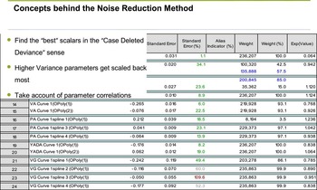
Figure 13 gives an example, that we call a ‘beta screen’. You do not need to read the numbers. All you need to know is that there is a list of parameters down one side, and then there is the value of the parameters that the model has decided are the best ones from using the normal GLM fit. The standard errors have been calculated and are shown. This particular piece of software colours them in for you in a helpful way: green is good; red is bad; grey is somewhere in between.

Figure 13

Parameter values with standard errors and weights

Basically, if the standard error is less than 50, then it colours it in green and says, “Yes, you can keep this one in your model” and the other ones drop out. So that is the current mechanism you might use to make a binary decision about parameters being in or out.

We decided that this Boolean ( In or Out ) decision was too primitive, and set ourselves the target of designing a method to scale the parameter by a percentage, probably between 0% and 100%.

The Case Deleted Estimates are a natural way to do this, and section 4.3 describes how Hat matrix acts as the Bayesian credibility combining the data point and the case deleted estimate into the full estimate.

The feature that we are trying to determine is: what are these best scalars? We observed that the standard error actually helps you make that decision and the standard error is obviously related to the variance that that parameter is adding into the model, with higher variance parameters are ones that you should probably drop out or scale back by a long way.

The other thing that you need to realise is that in most real world models you will find the parameters themselves are correlated with each other. You do not end up with a model with completely orthogonal parameters. In general, if you have lots of parameters in your model, some of them will overlap and they will be less than orthogonal. That means that if you move the value of one of the parameters, then in a normal generalised linear model all the other ones will then adapt to take account of that varied parameter.

So we need to be cognisant of that as well. If you scale back one of the parameters, you just cannot do so independently, you have to take account of all those covariances as well as the variances. Now, in section 4.3 of the paper you will see that we find a way of picking up the covariance matrix which the generalised linear model generates for us automatically, so it is a really great type of model to use because it generates all this for us. We have managed to find a way of relating the case deleted estimate to something that looks very like a Bayesian credibility related to this variance covariance matrix.

When you notice that, suddenly it all starts to fit together. It gives you a mechanism to remove this circular reference.

What we are proposing here is a two-step fitting process, as depicted in Figure 14. You take your sample data, you build up your model structure, and you press the fit button so you get your normal generalised linear model fit as you would do in everyday practice. Then you can do the case deleted method to calculate how well that model has fitted the data in this hold-out way of doing it.

Figure 14

Eureka the Circular Reference Resolved

Do not get confused here. I know Figure 14 has drawn sample data and hold-out data separately, but do not forget we have one dataset and we are rather cleverly using all of the data points in both of these places. It is just that we have used the hold-out sample by case deleting so it is independent of the calculation we are doing.

The second piece we want to do is to solve how much we should be scale back the parameters. We are using a mechanism here to do that that says if we have the variance covariance matrix, then that gets incorporated into the way that the case deleted estimate varies. It is to be hoped that we can do that in a way that does not produce a circular reference.

Figure 15 lists six equations.

Figure 15

Why scaling parameters has a stable optimum

Without tracing through all the maths, we start with a covariance matrix. From that you can get a hat matrix, in this case the hat diagonal. In the paper it shows that the case deleted estimate you have got is related to the normal estimate with this kind of Bayesian calculation here using the hat matrix. That is really nice because the hat matrix obviously takes account of all the variances and co-variances as we wanted it do.

This is where it all suddenly fits together and this gives the size of the case deleted adjustment. So a scaled version is easy to derive from high school statistics. These are worked through the GLM fitting algorithm shown in Appendix A, making adjustments to carry these new definitions through to allow the scalars to adjust to their optimum values using the case deleted deviance.

It seems that it is the fixing of the relationship between the parameter means and variances, which breaks the circular reference and allows the model to complete.

That is the theory. But there is no way of knowing that is going to work unless you actually try it out. More to the point, we want to know does this work for real insurance examples because we are actuaries, we do pricing and we are more interested in that than anything else.

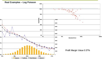
Here are some real examples. The first one is a Log-Poisson example, treated in the paper, and depicted in Figure 16. There are about 1 million rows of data in the model, 100-odd parameters in there, and it is reasonably realistic.

Figure 16

Case Study – Claim Frequency

What we have done, though, is that we have not taken that model right through to the current best practice of eliminating the parameters you normally drop out. I have left them in there, so you can see them there with standard errors of anything up to 100%, because then we can find out what the scalars would be for those values as well.

As I said earlier, you are expecting to scale between nought and 100% and this looks to be the case. You are also expecting the ones with the higher standard errors to be scaled back more. This seems to be true as well. Also in some circumstances, you will see correlated variables where they are obviously overlapping. You cannot see this from the chart but I think what is happening here is we have a couple of parameters that are doing roughly the same job. One obviously has a low variance and one has a high variance. The model is saying that instead of having 100% of both of those, you can do better by scaling the high variance one back and adding in a little bit more of the low variance one. In very rare circumstances, you can see that point is a parameter which has gained 102% of its starting value.

The chart in Figure 16 needs to be explained. It is probably not one that you might have seen before. What we wanted was a mechanism to value two competing models. In the normal world you might have a risk model that you used previously. Then you have a new one you have just built. What you want to know is which one is better. That is particularly useful in this case because we have our original GLM model, and we have our scaled GLM model.

You take the two models. You calculate the estimate for all of the rows of the hold-out sample, so independent of the dataset that you use to create the models in the first place. In this case, when I say hold-out sample, I am talking about a completely alternative second hold-out sample, different from the ones we talked about earlier in the paper which were being reused in a clever way. This is a second hold-out sample. For those estimates you obviously know the observations. You also know the estimates for both because you have just calculated them. You can calculate the ratio.

What the ratio gives you is a value of when the two models agree with each other, in which case the ratio would be nearer 100% in the middle, and when the two models disagree with each other. To work out which model is best you are most interested in places where the models disagree with each other. So what you then do is take the ratio you have calculated and divide it up into a series of bands. You can calculate the number of rows that fall into each of those bands. Then you can take the observations in that same way of bucketing, and you can calculate what the observed value would be. Then you can place for each of these different buckets the average estimate for the first model and the average estimate for the second model, and then what the average of the observed values is. The blue line in Figure 16 is the observed, the red line is our original GLM model, and the black line is our new noise reduced model.

What we can then do on top of that is use an assumed elasticity. This is a little bit more technical. It ends up generating one number which we can call a profit margin, which is a useful number to quote. So you say if these were the two sets of answers that you were going to come up with, and one model was selling business against another, you can use an elasticity model to say how much business would one model sell in each of these different places, and obviously where the model is quoting cheaper, it will sell more business. If it is quoting cheaper but still performing well against the observed, then it will outperform. If it is quoting more expensive, it will write less business, and if the observed are higher as well, then the model that sells the most business will make a loss. You can add it all up again and end up with a profit margin at constant volumes of business and say which one generates you a profit.

In the example underlying Figure 16, the model has added just over half a per cent of profit, which is a quite small amount. However, do not forget this mechanism is using the same data set that you already had before, and it is using the same kind of GLM techniques you already had before with an extra tweak at the end and so, in a sense, we are generating half a per cent of extra profit out of thin air. That cannot be bad, can it?

Our second example is a log-gamma and is depicted in Figure 17 using the same type of charts as our first example. I do not need to explain the charts again.

Figure 17

Case Study – Claim Severity

This model is a severity model of claims size that inherently has a lot more uncertainty in it because the gamma is a longer tail distribution. Rather pleasingly, you see that the higher standard error parameters are being scaled back by much larger amounts. There is still just one parameter there that squeaks in at just over 100, so that feature is still there. It seems to be quite a nice cascade as well. When you have very low standard error parameters, they seem to have scalars very close to 100%.

How much value does that one create? I think this chart is slightly easier to look at. I think you can see quite easily that the black lines outperform the red lines. That generates another half per cent of profit.

Do not forget if you are modelling frequency models and then severity models, then putting them together to generate your premium or risk model, that profit margin advantage is additive so you have gained a half in one place, you have gained another half in another place, so you must be at least 1% up.

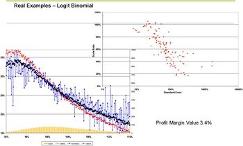
We have one more example. This is quite a topical one because injury claims have become a big problem in the current market. It is quite difficult to model injury claims, which are relatively sparse and very large and long-tailed. You generally find that your bodily injury frequency model has the least complexity of all the models. So one of the things that you could try doing instead to model your third party frequency model is to model collision frequency. Then you could build a propensity model on top of that to say what does the bodily injury data say that is different from the property damage model itself. That is what we have got in Figure 18, a propensity model of bodily injury divided by property damage.

Figure 18

Case Study – Propensity Model

You can see naturally that it is an awful lot more noisy, so the blue line is volatile. However, the noise-reduced model is out-performing the standard GLM by quite a large margin now, and if you were producing your risk models on this basis, it would be adding over 3% of profits to that particular part of your strategy. That could be quite important.

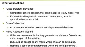
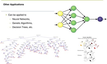
Let me make some final comments. Although we have talked exclusively here about applying these techniques to generalised linear modelling, I cannot think of any reason why these techniques could not be applied equally to other models as long as the model is generating parameters with mean values that you might accept, and it is possible to calculate some kind of variance and covariance measure from it. It just so happens that generalised linear modelling is very helpful and generates all those techniques for you and that machinery is available. However, with a little extra work, I am sure this approach could be applied to other places, see figure 19.

Figure 19

Other Applications

We think that the scale parameters, and the estimates that you can then build from that, will be the most predictive on your hold-out sample. Actually, that is extremely relevant for insurance because although we have historic data, and we have built models on historic data, that is not an end in itself. In actual fact, what you really want to do is work out what the patterns will be in next year's claims and use this information to go out and compete in the market. Naturally, next year's claims are a hold-out sample that you cannot currently see. Therefore you want to build the most predictive model against that unseen data. This is a technique that helps you to do that with your existing data and your existing modelling techniques, with a small tweak on top.

I conclude with Figure 20 which suggests that the techniques outlined in the paper might be applied to neural networks, decision trees or genetic algorithms.

Figure 20

Application to Other Models

Dr J. Janacek (visitor, University of East Anglia, opening the discussion): I am a statistician. I enjoyed the paper because it is an interesting but difficult topic. Statistics have revolutionised science but once you move out of the statistical paradigm – randomness, design, experiments – you move to shaky ground where inference can be a problem. I specialise in the study of time series, and it is obvious to me that most of traditional statistics is not a great deal of use.

If we talk about GLMs and the problems of inference then it seems there are two approaches.

One is to go down the route of the generalised linear mixed model, which is basically a more complex version of the traditional linear mixed model, which crops up a lot in biological and agricultural experiments. In this approach you take the generalised linear model predictors and add a random component with a pre-described covariance matrix. The idea is that you have heterogeneous clumps in your data and you use the randomness to try and smooth this out of the way. This approach is a possibility, but it is very complicated and you have to have a good deal of wisdom in how you put in your smoothing. Also, it is probably quite slow.

If you do not do that, then you have obviously got to go down the route of the authors, and you get down to the “leave one out” approach. This goes back a long way, back to at least the 1930s and possibly further back. The primitive idea was that you cannot really do much in traditional statistical terms, so what you do is you separate your data into a hold out sample and a fitting sample, machine learning call them test and training sets. You fit your model on the training set. You then predict the hold out sample and the discrepancy between the hold out sample and your predictions tells you something about how bad your model is.

This approach got modified over the years to K-fold leave outs, or K-fold cross-validation, where you take blocks of K observations. You take them out of your data, you fit the model and you then make predictions of the left out versions.

This approach is a little more complex, because there is the question of how do you choose the K, and if you are going to repeat this over and over again. This is why “leave one out” cross-validation is very nice because it is simple, it works fast, and there is no question about how you pick out a value. So leave one out validation seems good. What you do is take your data, leave out an observation, fit your model to the remaining, predict your left out observation; and the discrepancy, depending how you measure it, informs your choice of model. There is a good deal of work in this, in particular if you go back to classical regression – things like Cook's distance and leverage – where leaving out observations gives you some idea of outliers, and so on.

This is pretty well understood and I was going to say reasonably simple. If you generalise what we are talking about, to generalised linear models, the algebra is an extension of regression. The algebra looks like it works quite well.

I do have a question here. I would have some worries in using the R program because R is quite slow. If you have a lot of money you can buy bespoke software, so speed is not so much of a problem. I would be interested to know how long it takes for Mr Lovich to do these sort of exercises.

The interesting question is: how do you choose your discrepancy? You have made all these predictions and you know how bad they are. How do you bring these together? The authors have combined the change in deviance between two models with a change in deviance between two models on the hold out cases. They have taken a linear combination and a magic five has appeared from tuning it on data.

My hackles obviously rise. Where is the theory? I would be interested to have some idea of sensitivity and whether a linear assumption is really a sensible one.

There are other questions, and I will raise some of them now. My colleagues in machine learning have more or less stuck their colours to the mast of 10-fold leave outs. That is, they like to leave out blocks of 10. In my opinion their reasons may be mostly specious, but there is some theory which implies this might be a better way of going about things. It is more expensive. I would be interested to get the authors’ views.

I should also like to know a little bit about the value function, in particular how sensitive it is.

In addition, if you are fitting a model, you can step up or step down. I am a step down person. I fit everything and then delete them because that is what all sensible people do. Some people do step up. I would be interested to know whether which way you go is important in this case.

It is not my area of application, but I found the diagrams talking about the knots in 3.2.9 went way over my head. Again, I am a little suspicious. I was brought up in the era when pictures were lies and instruments of the devil and everything had to be in numbers. I do have problems about the diagrams. I would be interested to know how you would present this to people.

Then, to be quite frank, the noise reduction model I found very difficult. I actually understood a great deal more about it from this rather lucid presentation. Also, I did not work through all the algebra. That is probably part of my problem in understanding these things. It does appear to me that there is something of a free lunch here. I am sure that there is a cost involved. I would be interested to know that.

Probably more relevant is that, looking at the algebra, it seems to me that there is some sort of connection with the sort of algebra you get from fitting generalised mixed models. I wonder whether there is a coming together in some sense here, that in fact what I am thinking of as shrinkage for the noise reduction model is somehow related to the choice of covariance for the generalised mixed model. I am probably barking up the wrong tree, but we ought to leave a nasty question for the authors to look at.

I compliment the authors. It is a very interesting paper. It is really quite exciting to see what people are doing in a completely different subject, even if I do not understand all the implications.

Mr M. G. White, F.I.A.: My point is not at all technical. It is a professional question about the patent application which our chair mentioned.

I do not know whether this is a first: I have not noticed such a statement in any actuarial papers before. Under our Charter this Profession is set up as a public interest body and as a learned society, to share ideas and learn from each other, and it is important to reaffirm this from time to time. It is important that the precise context of the patent application is made clear or people might get the wrong impression.

If companies develop specific software applications, it is obvious that they are going to keep the intellectual property on them. But if there are ideas in a paper such as this which are meant to be shared, but in such a way that they may not be freely used afterwards, that would be an issue of concern.

Mr R. Kelsey, F.F.A.: Mine is mostly a technical contribution.

As Dr Janacek said, this technique is not new. It comes across in many guises called cross-validation or generalised cross-validation. There is some more material and more algebra in the bible of generalised additive models authored by Hastie and Tibshirani (1990). The part of the book easiest to read is that which treats the normal error, where they show that the form of the generalised cross-validation reproduces entirely the figure shown in Figure 3 and that shape of curve.

I would challenge Dr Janacek or the authors to try a little bit more analytics because I suspect that the factor 5 comes out analytically in the parameter value whereby you get zero at value five by totting up the approximate variances.

Reference

Hastie, T. J. & Tibshirani, R. J. (1990). Generalized Additive Models. Chapman and Hall.

Mr J. I. Iwanik, F.I.A.: I have two questions.

The chair mentioned a patent. Dr Janacek mentioned that the technique is well known and has been well known for years. How do these two things reconcile?

My second question is: will this technique detect multiple claims? For example if there is not just one outlier but a group of 1000 outliers, because there are two types of claims. Will this technique detect this type of problem?

Mr M. L. Sinclair-McGarvie (student): I have one general question and one technical question.

I am particularly interested in the generality of this procedure, as it appears to be a general alternative to the maximum likelihood approach that is particularly useful for improving predictive power in parameter estimation.

In my role currently I am focused on model calibration in a banking context, where there is a lot less data than in the authors’ applications. I wonder if the authors could comment a little bit more on general applications, possibly where there is less data and how we might test goodness-of-fit predictive power for this technique as opposed to other techniques?

Mr Lovick (responding): It is interesting to hear that the technique is not new. I agree cross-validation is not new. The mechanism of calculating case deleted estimates, for example, is in a book which is in one of the references of our paper.

However, the application of case deleted estimates to calculate a case deleted deviance and then to do the next step, which is the noise reduction technique, is not something I have seen anywhere else. I was challenging Dr Janacek to produce it in one of his books which, fortunately, he was not able to do. It is possible that, unknown to me, it is out there somewhere else in a book. That remains to be proved. To my knowledge to date, this is a unique technique.

The motivation for bringing this paper here is that we were asked to do so. Apparently, there have been many sessional papers at the Institute over the last few years, and almost none of them have been on the subject of general insurance. The subjects of life and pensions seemed to dominate. One of my colleagues at work, who happens to be on the committee for this, invited us to submit a paper that is relevant to practitioners in the general insurance industry. We are also hoping to share it with colleagues at the GIRO conference as well in October. That has yet to be validated by the committee.

Just one point on the detection of outliers: yes, I think case deletion originally came about as a means to delete single data points which were outliers in a data set. In an academic sense, if you have a dataset with 100 rows of data you may well go through and investigate and find out whether two or three of those are outliers and delete them. In the world in which we live, where you might have 10 million rows of data, in practice it is an extraordinarily laborious task to go through and search for outliers, and practically speaking you probably would not be able to remove, say, a few thousand of those by hand. So, that is exactly what this technique is designed to do – to find a mechanism to determine whether your model is depending on those outliers and, if it is, then to scale back those parameters and say that is just noise in the model and you should not be using that part of it.

Mr Lee (responding): I agree that the work has similar objectives to what Dr Janacek said earlier around generalised mixed models. In fact, there was a paper in the US last week on it.

But we feel that instead of assuming some sort of covariance, we are trying to use the data to estimate in a case deleted sense the scalar parameters. Maybe that is a distinction.

Mr S. K. Omar (student): When you remove a bunch of outliers, do you have to go back and re-look at all the interactions you fit, that are no longer valid? In your experience, have you had to do that quite a lot?

Mr J. I. Iwanik, F.I.A.: Do I understand correctly that for practical application this is like a better F-test? Compare two models and, like in the F-test, you will say that this model is worse than that. Case deleted deviance will instead say this model is better by so much, and maybe quantify the improvement so you can scale some coefficients back. Is my intuition right?

Another question: is a model which has lower case deleted deviance always better or is there a weight for the penalty like in GAM theory? Do you have to determine what the right weight for the penalty is, using something like the cross-validation, or is it just like: high deleted deviance, bad; low deleted deviance, good?

Mr Lovick (responding): First, I agree that commercial models are smaller and much more volatile and therefore the variances are going to be much larger. This technique should work perfectly there probably for all of the parameters you could ever include in a commercial model, and equally for Lloyd's markets syndicates, and whatever. If they have any data, then they are probably building small models that look very similar as well.

In the retail market, where you have lots of data, this effect will appear most at the frilly edges of the domain where your model is trying to extrapolate or becoming over-parameterised. It probably has very little effect in the centre of the domain where you have very stable estimates.

There was a question about removing outliers. In practice, with very large data sets, which I tend to work with, I do not personally remove outliers. The whole point of this technique is that it is automatically cycling through each of the data points and removing them for the purposes of using them as a hold out sample.

Mr Lee (responding): That is also the case when you look at frequency models and propensity models. Outliers do not really exist for the sparse data sets that we have. I agree that, potentially, you can use severity models but it is impractical and it does not tend to have too much of an impact.

Mr Lovick (responding): Regarding revalidating interactions: that is exactly what this method is doing in a sense because if the interaction becomes invalid then it will be scaling those parameters out. Perhaps not all the way to 0% but it is clearly telling you the interaction is not valid in that sense.

Let me answer the question about whether our test is a replacement for F-tests. In the chart that Mr Lee showed at the start of the presentation we compared it to the standard error there and its acceptance criteria if you were going to allow or exclude a parameter being higher or less than 50% standard error.

Then in the spline example, which admittedly is fairly artificial, we were looking at Chi squared and F-tests to find out whether it agreed in most circumstances. In the paper this test agrees with all of the simple cases where the Chi squared and the F-tests are also in agreement. In the one place where the Chi squared and F-tests disagree with each other, this test comes down in favour of one or other of those two.

Is it a replacement? Well, it is not quite the same as the F-test because the F-test is a mechanism that gives you a judgement on two models saying is this comparable to that. And also it is specifically operating in the case of nested models as well.

What I like about this mechanism is that, while it agrees with those in the case where that F-test is valid, it is also applicable in a wider sense as well because it is producing an absolute number that you can compare to a number of different models. It is the absolute value of that statistic that is useful in a wider context, not just nested models.

The second part of the question was about case deleted deviances. The answer is yes: in effect what we have done is notice the way that the variance/covariance matrix works through into the case deleted estimates and we have found a way of including that. It is like a penalty function. In a sense it is similar to the generalised linear mixed models that Dr Janacek referred to earlier. However, the difference is that the mixed models are simply arbitrarily adding on a penalty function in order to perturb the model back to the mean. There is no simple way to understand where that arbitrary parameter or the amount of smoothing that the person has added in has come from. Whereas, what we have done is come out with a theory using the case deleted estimates which, in effect, gives you that penalty in a natural way because it was determined from the data, that is a more sensible way of doing it. It avoids adding in any arbitrary parameters. That is the thing that makes it different from mixed models as they currently stand.

Mr Iwanik asked about the parameter of five. It is just a way of calibrating to make that value measure positive or negative if it is adding value. But that in itself is not used at all in the noise reduction technique. It is only the case deleted deviance which goes through to that. There are no arbitrary parameters in that at all. The data itself is producing the answer for you. That is what I see as the attractiveness of this method.

Mr M. L. Sinclair-McGarvie (student): It was mentioned several times that the case deleted deviance approximation is 99.99% accurate. To my knowledge, this is a linear approximation. It is, I presume, based upon a Taylor approximation.

How good it is on very much more convex problems, more non-linear problems? Also how good is it when you have got, as I queried earlier, less data? Is this 99.99% accurate figure coming from the number of data points that we are considering here? Would there be a less accurate approximation for this case deleted deviance used in the paper when we have fewer data points?

Dr J. Janacek (visitor, University of East Anglia): Having spent a career as a statistician, I no longer believe in F-tests. Cross-validation is the way to go.

I was very interested in generalised linear additive models but the estimation is really horrendous.

Based on simulations with cross-validation, if you go to K-fold as opposed to one-fold, you tend to get decreases in variance estimators and increases in bias as you increase the folding. Whereas in the case of for one-fold, leave one out, you get maximum variances. If you know nothing else, it is a wonderful technique, certainly if you want to make predictions.

Mr R. Kelsey, F.F.A.: I re-read Hastie and Tibshirani and my understanding, certainly for the splines, was that the AIC criterion was effectively the same as the generalised cross-validation to first order, which would also hence be similar with the F-tests. However, these are all first order approximations. I would be more interested to see where one method favours one approach against another.

Going back to Dr Janacek's point on the K sample leave out, the question for us in the general insurance environment is how to do that quickly on a large data set. Also, the large data sets are often sorted in terms of their covariates, so if you take consecutive samples, there could be a lot of unintended correlation within that approach.

Mr Lee (responding): On Mr Kelsey's point, there is a penalty function in AIC, which is not likely unless the number of parameters is small. My problem with that is the units are mismatched. I see the penalty as slightly arbitrary. What our value function does is try to use the data in a cross-validation way, which appears to come out with a more robust validation test for comparing even non-nested models.

Mr Lovick (responding): Mr Sinclair-McGarvie questions the 99.9% approximation. We have tested that in some reasonably different sized datasets in the three examples we have given, so the frequency one had 1 million rows, there was another one with 100,000 or maybe slightly smaller. So we have spanned an order of magnitude in data size. We got roughly the same number out of those two. That is a very small sample of different datasets. Clearly there is more work to be done to investigate other datasets and find out whether that number changes with different model types, or more complex ones. So I do agree with you completely.

The approximation we have chosen is a first order effect that gets you to the estimate that we have come up with there.

That is probably the crux of this matter about leaving out one or leaving out 10 that Dr Janacek was talking about earlier. For example, if you had maybe 100 rows of data, leaving out 10 would be a quite different effect than if you had 10 million rows of data and you left out 10 at a time, which would probably have no more effect than leaving out one. So “why 10?” I would say, “Why not 100 or 1000 or some proportion of the dataset that you are leaving out instead?”

But equally I would like to agree that once you leave out more than one the question arises: how do you do this without refitting the model? Obviously, you could leave out 10 or 100 data points and then refit the model. That is possible. But with very large datasets you cannot physically go through all of those possibilities and fit the model that many times, which is why we settled on a leave out one and then use an approximation because that shortcuts the whole process and gives us a practical way of doing the calculations.

Also, if you were leaving out 10, then you would have to make sure that they were not correlated with each other, so you could not simply go through the dataset in order. You would have to find some way of randomising the 10 that you chose. That again will be interesting because if you are doing a random method of how to choose the 10 to leave out, then your answers may not be replicated if you run the same model again because you may have a different set of 10 next time. Whereas with the leave out one at a time at least that is uncontroversial in the sense that you can replicate the same answer the second time round.

The Chair (Mr S. M. Shepley, F.I.A.): We are fortunate tonight that Dr David Brown has agreed to close this discussion. Before I ask him to conduct that role, I note that one topic not covered is an earlier one about speed. Are there any points for us, as a learned society, that you want to make on the topic of the practicality of actually using this model?

Mr Lee (responding): The algorithms used to fit these models obviously have a factor on speed. Speed is gained by essentially optimising the algorithms you are using to fit the model in general insurance rather than trying to be all things to all men.

Dr W.D. Brown, F.I.A. (closing the discussion): I have had the opportunity to have several conversations with Mr Lovick and Mr Lee before this evening to discuss the paper. At times I have been absolutely intrigued and at other times completely baffled.

It is clear to me that there is genuine novelty here. Today has offered us a very useful opportunity to assess some of the techniques that can be employed in the work that we do every day in general insurance pricing and to extend it rather than just blindly continuing with the same techniques, because we have used them before.

The challenge here is to think out of the box – in fact to think beyond the black box. There is a part of me that is rather wishing that all of this complexity would get back in the black box so that we can resume turning the handle on it very quickly!

One of the things that has come up again and again is data complexity– one aspect of this is outliers. While when we look at simple datasets it is fairly obvious what the outliers are, in the huge complex datasets that we work with, it is not entirely clear what they are, or even how we might identify them. So it is fascinating to have a technique that will in some sense identify them.

It would not mean very much if the algorithm set out by Mr Lovick and Mr Lee did not have speed. It will be very interesting to test that out in earnest.

While it is always intriguing and tempting to try to get the most out of any data set, I do have some reservations. We always need to challenge ourselves with questions. For example: do we actually have the right data? Do we have the right variables that are describing the problem? In fact, are we trying to solve the right problem at all? When we look to some of the applications where we most want to use it – situations of aggregators with the Winner's Curse problem, bodily injury claims, banking, commercial insurance with sparse data or the Lloyd's market – I suppose we need to be very careful that we ask ourselves the intelligent questions. Do we have the right information before we turn to modelling?

I commend Mr Lovick and Mr Lee on an intriguing paper and I look forward to seeing how it fares in our practical work.

The Chair (Mr S. M. Shepley, F.I.A.): It remains for me to make a vote of thanks. Thank you very much to the authors. You will agree that they have had the courage and the commitment to put themselves up here and put forward some thought-provoking ideas which are not conventional.

In this particular busy time for all of us, particularly with what is happening in Europe on a regulatory and a pricing perspective, I should like to thank them personally for taking the time.

I very much look forward to revisiting this topic at GIRO. We should definitely be considering it further. It perhaps lends itself to a number of interactive sessions as well. We will take that thought away.

I also thank Dr Janacek and Dr Brown for opening and closing and also all of you in the room for being attentive and participating.

Written contribution from Mr Richard Kelsey, F.F.A. following the meeting:

The concepts introduced in sections 5 and 6 of the paper are not new to statistical literature. Other research should have been referenced and can be found if one searches under the more common description of ‘shrinkage regression’. Indeed it was only after the paper was read that I made the link between the paper presented and statistical papers on shrinkage. There is a vast amount of research on this topic, much of which was published in the 1980s and 1990s. Van Houwelingen (2001) is a very readable and useful review paper which serves as a non technical introduction to the topic. In brief summary:

1. 1. Shrinkage regression reduces the prediction mean square error and overfitting by reducing the parameter estimates via a shrinkage factor or vector. This is at the cost of introducing a small bias to the estimator.

2. 2. There are a number of different shrinkage parameterisations and different approaches to choosing the optimal amount of shrinkage. Whilst generalised cross validation (GCV) or AIC are common approaches, they are not always best. Simulation examples can be generated where such approaches are negatively correlated with the true optimal shrinkage parameter.

3. 3. Shrinkage regression can be recast as a penalised regression model. Whilst some penalty functions (or constraints) can appear arbitrary, others result from the appropriate choice of a Bayesian prior for the parameters. Simulating such distributions results in Generalised Linear Mixed Models (GLMMs) which potentially solve the problem of poor choices of smoothing parameters introduced by GCV or AIC minimisations.

Whilst GLMMs will not cope with the size of datasets common for personal lines insurance frequency analyses, they are potentially feasible for severity analysis, and analysis of commercial lines datasets. Research into shrinkage continues, most notably in the field of Generalised Additive Models (GAMs), e.g. Wood (2011). Models and new research are often implemented via the free to download R software in contributed packages such as mgcv.

In summary, I congratulate the authors for bringing these topics to the notice of the actuarial professional and providing the motivation for using such methods in a non-technical discovery-type paper but would welcome further work, perhaps via a GIRO working party, to digest, investigate and identify which of the other available approaches work best on insurance data.

References

R Development Core Team (2009). R: A language and environment for statistical computing. R Foundation for Statistical Computing, Vienna, Austria. ISBN 3-900051-07-0. http://www.R-project.org.

Van Houwelingen, J.C. (2001). Shrinkage and penalised likelihood as methods to improve predictive accuracy. Statistica Neerlandica, 55, 17–34.

Wood, S.N. (2011). Fast Stable restricted maximum likelihood and marginal likelihood estimation of semiparametric generalized linear models. J R Statist. Soc B, 73, 3–36.

Wood, S.N. (2011) mgcv: GAMs with GCV/AIC/REML smoothness estimation and GAMMs by PQL. Available in Packages areas of R Website, http://www.R-project.org.

Authors reply to written contribution from Mr R. Kelsey, F.F.A.