





1 Introduction
The analysis of intensive longitudinal data (ILD) is a rapidly growing area in behavioral and social sciences (Ariens et al., Reference Ariens, Ceulemans and Adolf2020; Bolger & Laurenceau, Reference Bolger and Laurenceau2013; Hamaker, Reference Hamaker2025; Hamaker et al., Reference Hamaker, Ceulemans, Grasman and Tuerlinckx2015; Walls & Schafer, Reference Walls and Schafer2006). Its primary aim is to understand processes and behaviors as they unfold over time. Unlike traditional longitudinal or panel data, which typically involve a few evenly spaced observations (e.g., annually over a couple of years), or time series studies that focus on a single unit, ILD are collected from multiple units at many time points (e.g., tens, hundreds, or sometimes even thousands). ILD studies are characterized by a relatively high temporal resolution compared to the time frame of the study (e.g., hourly assessments during daytime over a week), allowing researchers to closely track changes over time and analyze patterns and dynamics that might be missed in studies with less frequent measurements (Walls & Schafer, Reference Walls and Schafer2006).
In psychology, ILD are often collected using methods, such as the experience sampling method (ESM; Tuerlinckx et al., Reference Tuerlinckx, Kuppens, Ariens, Cloos, Dejonckheere, Lafit, Niemeijer, Revol, Schat, Schreuder, Vanhasbroeck and Ceulemans2025), ecological momentary assessment (EMA; Stone & Shiffman, Reference Stone and Shiffman1994), or ambulatory assessment (AA; Trull & Ebner-Priemer, Reference Trull and Ebner-Priemer2020), which capture real-time data on individuals’ experiences, behaviors, and physiological states in naturalistic settings. For example, researchers in the life sciences and psychology can nowadays easily collect massive amounts of data in real-time using devices used to monitor health behaviors (e.g., medication adherence and physical activity), psychological states (e.g., mood and stress), and physiological responses (e.g., heart rate and sleep patterns).
An example of an ILD study that we will further analyze in detail in this article is the Exam Results Study by Kalokerinos et al. (Reference Kalokerinos, Erbas, Ceulemans and Kuppens2019; see also the next section). In this study, a sample of first-year university students self-reported their negative affect on a visual analog scale multiple times per day for nine consecutive days, some days before and after receiving their exam results (which is, for most students, a stressful and important event).
Based on the example, we can describe some key features of ILD that have implications for the way the data are being analyzed. First, it inherently possesses a multilevel structure. For instance, measurements (Level 1) might be repeatedly collected within the same day (Level 2), with multiple such assessment days for each individual (Level 3). Consequently, modeling ILD necessitates the distinction and estimation of variance components associated with these different hierarchical levels, such as between-person, between-day (or within-person), and within-day variances. Second, due to the high temporal resolution typical of ILD, successive observations are often correlated. This characteristic contrasts with traditional modeling approaches that often assume independence among observations.
Despite the rising popularity of studies with ILD, evaluating the reliability of measurements in ILD is often neglected or carried out inappropriately. This holds both for the reliability of measurements with single items (Dejonckheere et al., Reference Dejonckheere, Demeyer, Geusens, Piot, Tuerlinckx, Verdonck and Mestdagh2022; Schuurman & Hamaker, Reference Schuurman and Hamaker2019; Schuurman et al., Reference Schuurman, Houtveen and Hamaker2015) and for measurements with multiple indicators (Brose et al., Reference Brose, Schmiedek, Gerstorf and Voelkle2020; Calamia, Reference Calamia2019; Castro-Alvarez et al., Reference Castro-Alvarez, Bringmann, Back and Liu2025; Marcoulides, Reference Marcoulides2019). The use of a single item to measure constructs in ILD is driven by the need to minimize participant burden from frequent assessments (Dejonckheere et al., Reference Dejonckheere, Demeyer, Geusens, Piot, Tuerlinckx, Verdonck and Mestdagh2022; Wilhelm & Schoebi, Reference Wilhelm and Schoebi2007). Obviously, a critical liability of single-item measures is their heightened susceptibility to measurement error (Sarstedt & Wilczynski, Reference Sarstedt and Wilczynski2009). Although any observed score is unavoidably tainted by measurement error, averaging over several observed scores tends to improve the signal-to-noise ratio and thus reliability. However, this is not an option for single-item measures, and therefore, the evaluation of reliability is all the more important.
In addition, the two aforementioned key characteristics of ILD studies (i.e., the multilevel nature and time dependency) provide a further challenge to the accurate evaluation of reliability. First, addressing the multilevel structure is essential for accurate reliability estimation in ILD. There are approaches to estimate reliability at each level of the multilevel structure, such as generalizability theory (GT; Cranford et al., Reference Cranford, Shrout, Iida, Rafaeli, Yip and Bolger2006; Lin et al., Reference Lin, Tuerlinckx and Vanbelle2025; Nezlek, Reference Nezlek2017; Shrout & Lane, Reference Shrout, Lane, Cooper, Camic, Long, Panter, Rindskopf and Sher2012b; ten Hove et al., Reference ten Hove, Jorgensen and van der Ark2022) and multilevel SEM (Castro-Alvarez, Tendeiro, de Jonge, et al., Reference Castro-Alvarez, Tendeiro, de Jonge, Meijer and Bringmann2022; Geldhof et al., Reference Geldhof, Preacher and Zyphur2014; Koch et al., Reference Koch, Jaehne, Riediger, Rauers and Holtmann2025; Lai, Reference Lai2021; Nacke & Mayer, Reference Nacke and Mayer2025; Xiao et al., Reference Xiao, Wang and Liu2023). However, in practice, many researchers still resort to grabbing a single global reliability metric (e.g., Cronbach’s alpha) or only consider between-person indices, improperly ignoring the within-person variance. This oversight can lead to inaccurate and potentially misleading estimates of reliability (Calamia, Reference Calamia2019; Castro-Alvarez et al., Reference Castro-Alvarez, Bringmann, Back and Liu2025; Schuurman & Hamaker, Reference Schuurman and Hamaker2019; Vogelsmeier et al., Reference Vogelsmeier, Jongerling and Maassen2024).
Second, estimating reliability in (intensive) longitudinal studies is particularly challenging because conventional methods (e.g., test–retest) presume that reliability remains static over time. However, in ILD, this assumption is often violated due to the dynamic nature of the constructs being measured and the presence of serial correlation among repeated measurements. Consequently, the serial correlation among repeated measurements is often neglected when estimating reliability (Marcoulides, Reference Marcoulides2019; Molenberghs et al., Reference Molenberghs, Laenen and Vangeneugden2007; Revelle & Condon, Reference Revelle and Condon2019; Vangeneugden et al., Reference Vangeneugden, Laenen, Geys, Renard and Molenberghs2004, Reference Vangeneugden, Laenen, Geys, Renard and Molenberghs2005). While this oversight might have a negligible impact on estimating the internal consistency of multi-item measures (e.g., Castro-Alvarez et al., Reference Castro-Alvarez, Bringmann, Back and Liu2025), it can lead to biased reliability estimates for the test–retest reliability of single-item measures, because the systematic variance due to temporal dependency is incorrectly attributed to either true score variance or measurement error. Therefore, establishing and reporting appropriate reliability metrics is an imperative step before utilizing ILD measures in practice. It is essential to develop and refine methods for estimating reliability that are tailored to the complex, dynamic, multilevel data structures inherent in intensive longitudinal studies.
To address these issues, reliability can no longer be a single coefficient (Castro-Alvarez et al., Reference Castro-Alvarez, Bringmann, Back and Liu2025; Tisak & Tisak, Reference Tisak and Tisak1996; Vangeneugden et al., Reference Vangeneugden, Laenen, Geys, Renard and Molenberghs2004); instead, it should be assessed at multiple levels and across different time scales. In this article, two distinct yet related approaches will be used to define reliability coefficients in ILD: the correlation approach (e.g., Bartko, Reference Bartko1966; Lin et al., Reference Lin, Tuerlinckx and Vanbelle2025; Lord et al., Reference Lord, Novick and Birnbaum1968; Shrout & Fleiss, Reference Shrout and Fleiss1979; Vangeneugden et al., Reference Vangeneugden, Laenen, Geys, Renard and Molenberghs2004, Reference Vangeneugden, Laenen, Geys, Renard and Molenberghs2005) and the variance partitioning approach (e.g., Castro-Alvarez, Tendeiro, de Jonge, et al., Reference Castro-Alvarez, Tendeiro, de Jonge, Meijer and Bringmann2022; Hunter, Reference Hunter2026; Laenen et al., Reference Laenen, Alonso and Molenberghs2007; Laenen et al., Reference Laenen, Alonso, Molenberghs and Vangeneugden2009b; Schuurman & Hamaker, Reference Schuurman and Hamaker2019; Xiao et al., Reference Xiao, Wang and Liu2023). The first approach views reliability as the consistency or agreement of measurements across different occasions (e.g., measurements of different persons and measurements of the same person at different time points). The variance partitioning approach conceptualizes reliability as a variance ratio, addressing the extent to which an instrument can distinguish systematic or target variance from measurement error. We will formally introduce these two approaches in the later sections.
Our multifaceted approach results in various reliability measures that capture the properties of measurements from two distinct perspectives: (1) between-person versus within-person level and (2) stability across different time spans. For the first perspective, at the between-person level, reliability quantifies how well the measurement instrument distinguishes among individuals, separating true trait differences from measurement error. At the within-person level, it assesses how well the instrument tracks an individual’s true state fluctuations over time. The second perspective concerns temporal similarity (i.e., test–retest reliability) across different time lags, such as moment-to-moment within the same day, day-to-day, or even longer intervals. While the relation between the correlation and variance partitioning approaches is not clear at first sight because of differences in starting points and equations, we will analyze their interrelatedness and provide an integrated framework.
To sum up, the goal of this article is to define and estimate various reliability measures for the single-item measurements in ILD, taking into account its multilevel structure and serial correlation among repeated measurements. To achieve this, we propose to use a general three-level linear mixed-effect model (LMM) with the autoregressive process to appropriately distinguish different sources of variance. Based on our illustration example (the Exam Results Study), specifically, these variance components may come from between-person differences, within-person differences across days, serial correlation at the day level and the moment level, and measurement error. Building upon this model, we then define and interpret reliability at different hierarchical levels and time spans by the correlation and variance partitioning approaches. Furthermore, we will demonstrate what the reliability coefficients will be when our approach is applied to a number of commonly used models in (intensive) longitudinal research that are special cases of our general three-level model, including the two-level LMM with/without autoregressive processes and the three-level LMM without autoregressive processes. This systematic evaluation will reveal how different model specifications determine the resulting single-item reliability coefficients and will provide researchers with a comprehensive understanding of how to assess reliability in various ILD contexts. Finally, these approaches will be illustrated on the Exam Results Study using a Bayesian framework.
2 Motivating example: The Exam Results Study
In the Exam Results Study, Kalokerinos et al. (Reference Kalokerinos, Erbas, Ceulemans and Kuppens2019) investigated the dynamics of affect of 101 Belgian first-year psychology students at KU Leuven (87 women; age: M = 18.6;
$SD$
 = 1.5) before and after they received their first-semester exam results (covering five courses). The primary focus of the original study was on how emotion regulation differs across individuals. Such emotion regulation strategies need to be employed when receiving these exam results. These results are particularly significant for freshman students, because the first year is considered to be a selection year in the Belgian university system. Thus, receiving the exam results is a highly personally relevant and real-life event compared to experimental studies of emotional regulation.
In this study, each student (level 3) was tracked for nine consecutive days (level 2) using experience sampling. Within each day, a momentary survey was administered using a stratified random interval scheme from 10 a.m. to 10 p.m. (level 1). The total number of measurement times is 90. The exam results were released on the third day between the 21st and 28th measurement times. Students self-reported their affect on a visual analog scale ranging from 0 (= not at all) to 100 (= very much) for various items related to specific emotions and emotion-regulation strategies. In this article, we focus on the single item measuring negative affect: “Please indicate how negative you are feeling right now.” The average compliance rate, defined as the percentage of completed momentary assessments for each student, was generally high, with a mean of 90.8% (
$SD$
 = 7.4%, min = 64.4%, max = 100%).
A researcher collecting these data or a critical consumer of this research may wonder: (1) To what extent can persons be distinguished from one another over an extended period of time? (2) To what extent would repeating the measurement at exactly the same given moment yield a similar result? and (3) How does the agreement between measurements change across varying time intervals? These questions illustrate different reliability assessments that can be computed for this data set.
3 Three-level linear mixed-effect model with autoregressive processes
Univariate LMMs have been widely used in ILD studies to model single-item measurements while taking into account the multilevel structure and the serial correlation (Lodewyckx et al., Reference Lodewyckx, Tuerlinckx, Kuppens, Allen and Sheeber2011; Ma et al., Reference Ma, Mermelstein and Hedeker2020; Nezlek, Reference Nezlek2007; Vansteelandt & Verbeke, Reference Vansteelandt and Verbeke2016; Verbeke & Molenberghs, Reference Verbeke and Molenberghs2000; Walls & Schafer, Reference Walls and Schafer2006). As an analysis model for the Exam Results Study, we propose to use the model proposed by Ma et al. (Reference Ma, Mermelstein and Hedeker2020). This is a three-level LMM along with autocorrelated innovations at both the moment and day level.Footnote 1
Let
$y_{ijk}$
 be the observed measurement (e.g., a negative affect rating) for person
$i = 1, \dots , N$
 on day
$j = 1, \dots , D$
 at moment
$k = 1, \dots , M$
 , assuming a balanced design.Footnote
2
The model is defined by the following three levels:


At level 1, the observation
$y_{ijk}$
 is modeled as three components. First,
$\mu _{ij}$
 is a mean state of person i on day j. Second,
$\omega _{ijk} \sim \mathcal {N}(0, \tau _m^2)$
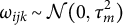 is a moment-to-moment serial process effect. It captures within-day serial dependence and is modeled as an AR(1) process, where
$\tau _m^2$
 is the stationary variance of the process. The covariance structure of
$\omega $
 ’s on the same day is
$\operatorname {\mathrm {Cov}}(\omega _{ijk}, \omega _{ijk'}) = \tau _m^2 \phi _m^{|k - k'|}$
 ,Footnote
3
where
$|\phi _m| < 1$
 is the autoregressive parameter, indicating how much carry-over there is from the previous moment to the current one. Third,
$\varepsilon _{ijk} \sim \mathcal {N}(0, \sigma _{\varepsilon }^2)$
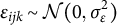 is the momentary measurement error. The errors are assumed to be mutually independent, and the error variance
$\sigma _\varepsilon ^2$
 (similarly for
$\tau _m^2$
 ) is assumed to be homogeneous across all time points (moments and days) and persons.
At level 2, the daily mean state
$\mu _{ij}$
 is also decomposed into three components. First,
$\mu _i$
 is the mean state of person i. Second,
$\nu _{ij} \sim \mathcal {N}(0, \tau _d^2)$
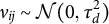 represents a day-level AR(1) serial process across consecutive days, where
$\tau _d^2$
 is the stationary variance of the serial process. The covariance structure of
$\nu $
 ’s is
$\operatorname {\mathrm {Cov}}(\nu _{ij}, \nu _{ij'}) = \tau _d^2 \phi _d^{|j - j'|}$
 , where
$|\phi _d| < 1$
 is the autoregressive parameter for the day level. By specifying the autoregressive process, similar to level 1, we account for the systematic carry-over effect from one day to the next. Third,
$d_{ij} \sim \mathcal {N}(0, \sigma _{d}^2)$
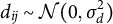 is a random effect for day (nested within person i). For simplicity, the variance of the day-specific deviations,
$\sigma _{d}^2$
 , is assumed to be homogeneous across days and persons.Footnote
4
Finally, at level 3, the person-mean
$\mu _{i}$
 is modeled as the sum of
$\beta _0$
 , an overall grand mean (a fixed effect) for the population, and
$s_i \sim \mathcal {N}(0, \sigma _s^2)$
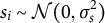 , a random effect for person i. Note that all three levels are assumed to be mutually independent.
Combining Equations (3.1)–(3.3) yields the single-equation form of the model:

3.1 Marginal model and covariance structure
In general, Equation (3.4) can be expressed as a vectorized expression for each person i as follows:

where
$\boldsymbol {y}_i = \left ( y_{i11}, \dots , y_{i1M}, y_{i21}, \dots , y_{iDM} \right )^\top $
 is a vector with all observed measurements for person i.
$\boldsymbol {X}_i$
 ,
$\boldsymbol {Z}_i^{(s)}$
 ,
$\boldsymbol {Z}_i^{(d)}$
 , and
$\boldsymbol {Z}_i^{(\nu )}$
 are the design matricesFootnote
5
for the fixed effect (vector)
$\boldsymbol {\beta }_i = \beta _0$
 and the person random effect (vector)
$\boldsymbol {s}_i = s_i$
 , person random effect (vector)
$\boldsymbol {d}_i = (d_i, \dots , d_D)^\top $
 , and the day-level serial effect (vector)
$\boldsymbol {\nu }_i = (\nu _{i1}, \dots , \nu _{iD})^\top $
 , respectively.
$\boldsymbol {X}_i$
 and
$\boldsymbol {Z}_i^{(s)}$
 are a column vector of ones with length
$DM$
 , and
$\boldsymbol {Z}_i^{(d)}$
 and
$\boldsymbol {Z}_i^{(\nu )}$
 are
$\underset {D \times D}{\boldsymbol {I}} \otimes \underset {M \times 1}{\boldsymbol {1}}$
 , where
$\boldsymbol {I}$
 is an identity matrix with diagonal elements equal to one, and zero elsewhere, and
$\boldsymbol {1}$
 is a column vector of ones. The operator
$\otimes $
 denotes the Kronecker product. Under the balanced design assumption, everyone has the same number of measurements, so the design matrices
$\boldsymbol {X}_i$
 ,
$\boldsymbol {Z}_i^{(s)}$
 ,
$\boldsymbol {Z}_i^{(d)}$
 , and
$\boldsymbol {Z}_i^{(\nu )}$
 are the same for all persons i. The remaining vectors
$\boldsymbol {\omega }_i = (\omega _{i11}, \dots , \omega _{i1M}, \omega _{i21}, \dots , \omega _{iDM})^\top $
 and
$\boldsymbol {{\varepsilon }}_i = ({\varepsilon }_{i11}, \dots , {\varepsilon }_{i1M}, {\varepsilon }_{i21}, \dots , {\varepsilon }_{iDM})^\top $
 collect moment-level serial effects and measurement errors, respectively. Compared to a standard LMM formulation, Equation (3.5) explicitly distinguishes the serial processes
$\boldsymbol {\nu }_i$
 and
$\boldsymbol {\omega }_i$
 from the measurement error
$\boldsymbol {{\varepsilon }}_i$
 , to stress that the fluctuation of within-person observations could come from two personal dynamical processes instead of coming from the measurement random errors (Diggle, Reference Diggle1988; Ma et al., Reference Ma, Mermelstein and Hedeker2020; Verbeke & Molenberghs, Reference Verbeke and Molenberghs2000).
The total (co)variance of the marginal model (Equation (3.5)), denoted
$\boldsymbol {V} = \operatorname {\mathrm {Var}}(\boldsymbol {y}_i)$
 , is the sum of the covariance matrices of the random components:

Each component in this decomposition represents a distinct source of variation:
$\boldsymbol {\Sigma }_S = \sigma _s^2 \underset {DM \times DM}{\boldsymbol {J}}$
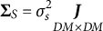 , where
$\boldsymbol {J}$
 is a matrix with all elements equal to 1, represents the person-specific covariance matrix, accounting for the between-person variation between their effects;
$\boldsymbol {\Sigma }_D = \sigma _d^2 \underset {D \times D}{\boldsymbol {I}} \otimes \underset {M \times M}{\boldsymbol {J}}$
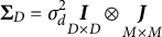 represents the day random effect variance;
$\boldsymbol {\Sigma }_{\nu } = \tau _d^2 \underset {D \times D}{\boldsymbol {H}_d} \otimes \underset {M \times M}{\boldsymbol {J}}$
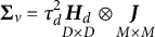 represents the covariance between day-level serial process, following the AR(1) structure;
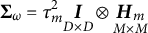
$\boldsymbol {\Sigma }_{\omega } = \tau _m^2 \underset {D \times D}{\boldsymbol {I}} \otimes \underset {M \times M}{\boldsymbol {H}_m}$
 represents the covariance between moment-level serial process; and, lastly,
$\boldsymbol {\Sigma }_E = \underset {D \times D}{\boldsymbol {I}} \otimes \sigma _{\varepsilon }^2\underset {M \times M}{\boldsymbol {I}} = \sigma _{\varepsilon }^2 \underset {DM \times DM}{\boldsymbol {I}}$
 .
The distinction between the day-related components,
$\boldsymbol {\Sigma }_D$
 and
$\boldsymbol {\Sigma }_\nu $
 , becomes clearer when examining their underlying structures at level 2 (see Equation (3.2)) and examining their respective covariance matrix structures:

$\boldsymbol {H}_d$
 depicts the autocorrelation of daily fluctuation based on the AR(1) process. In contrast,
$\operatorname {\mathrm {Var}}(\boldsymbol {d_i})$
 captures the residual variance of these daily fluctuations that is not captured by the serial correlation.
Similarly, the difference between
$\boldsymbol {\Sigma }_{\omega }$
 and
$\boldsymbol {\Sigma }_{E}$
 , both at level 1 (see Equation (3.1)), can be understood by examining their covariance matrix structures:

In this context,
$\boldsymbol {H}_m$
 depicts the autocorrelation of momentary fluctuation based on the AR(1) process, while
$\operatorname {\mathrm {Var}}(\boldsymbol {{\varepsilon }}_{ij})$
 captures the residual variance at each moment that is not explained by the serial correlation or other variation accounted for in the model.
Finally, the total variance of observations for a specific person i, conditional on that person, can be expressed as

for
$i = 1, \dots , N$
 . Conditioning on i emphasizes that the focus is solely on person i, thereby removing the person variance component in Equation (3.7). This distinction is fundamental for defining reliability later: the total variance
$\boldsymbol {V}$
 will be used when discussing the between-person reliability, while the person-specific variance
$\boldsymbol {V}_i$
 will be used when discussing the within-person reliability.
4 Reliability for intensive longitudinal studies
Before discussing how to define reliability for ILD, we briefly revisit the concept of reliability in the context of classical test theory (CTT). We will introduce two complementary approaches to define and interpret reliability: the variance partitioning and correlation approaches. We then introduce the reliability coefficients under the LMM framework defined in Section 3 based on these two approaches, extending from the existing literature.
4.1 Reliability in CTT
The concept of reliability in psychometrics originates from CTT (Lord et al., Reference Lord, Novick and Birnbaum1968). In CTT, it is assumed that the observed score
$y_{it}$
 for individual i at timeFootnote
6
t can be decomposed into an individual true score
$T_{i} = \operatorname {\mathrm {E}}[y_{it}]$
 and a measurement error
${\varepsilon }_{it}$
 , that is,
$y_{it} = T_{i} + {\varepsilon }_{it}$
 . Assuming that the true score and error are uncorrelated and that errors are mutually independent, the variance of the observed score can be partitioned as
$\sigma _y^2 = \sigma _T^2 + \sigma _{\varepsilon }^2$
 , where
$\sigma _T^2$
 is the true score variance, and
$\sigma _{\varepsilon }^2$
 is the measurement error variance. Consequently, reliability is defined as the squared correlation (or coefficient of determination) between the observed score and the true score across the population:

which simplifies to the ratio of the true score variance to the total observed score variance.
This definition can be seen as an instance of a more general principle: the variance partitioning approach. Under this approach, the total variance of the observations is separated into a systematic and an unsystematic part, and then reliability is defined as a ratio of the systematic variance over the total variance (Cranford et al., Reference Cranford, Shrout, Iida, Rafaeli, Yip and Bolger2006; Cronbach, Reference Cronbach1972; Ghiselli et al., Reference Ghiselli, Campbell and Zedeck1981; Guttman, Reference Guttman1945; Laenen et al., Reference Laenen, Alonso and Molenberghs2007; Laenen et al., Reference Laenen, Alonso, Molenberghs and Vangeneugden2009a, Reference Laenen, Alonso, Molenberghs and Vangeneugden2009b; Lord et al., Reference Lord, Novick and Birnbaum1968; McDonald, Reference McDonald1999; McGraw & Wong, Reference McGraw and Wong1996; Schuurman & Hamaker, Reference Schuurman and Hamaker2019; Shrout & Lane, Reference Shrout, Lane, Mehl and Conner2012a; ten Hove et al., Reference ten Hove, Jorgensen and van der Ark2022). Systematic variance refers to score changes that are attributed to identifiable and often predictable influences—such as stable individual differences or an orderly pattern change in some trend. In contrast, unsystematic variance stems from random, unpredictable fluctuations, including noise characterized by a complete absence of order. This unsystematic variance constitutes the primary source of measurement error. Thus, the general formula for reliability under this approach is

where the subscripts
$\text {sys}$
 and
$\text {unsys}$
 indicate the systematic and unsystematic variance components, respectively. Within the CTT framework, the systematic variance is the true score variance, and the unsystematic variance is the error variance. Consequently,
$R = \frac {\sigma _T^2}{\sigma _T^2 + \sigma _{\varepsilon }^2} = \rho _{yT}^2$
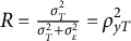 . Conceptually, this coefficient quantifies the ability of a measurement instrument to differentiate between individuals despite the presence of measurement errors across the population. Assume two persons, A and B, and the observed score of A is higher than that of B. The higher the reliability, the more confidence we have in inferring that person A’s true score is also larger than person B’s true score.
Alternatively, there is a second approach to define reliability, denoted as the correlation approach. Under this approach, one defines reliability as a correlation between two parallel measurements of the same individuals (e.g., repeated administrations of the same test or administrations of strictly parallel forms) (Bartko, Reference Bartko1966; Lin et al., Reference Lin, Tuerlinckx and Vanbelle2025; Lord et al., Reference Lord, Novick and Birnbaum1968; Molenberghs et al., Reference Molenberghs, Laenen and Vangeneugden2007; Shrout & Fleiss, Reference Shrout and Fleiss1979; Vangeneugden et al., Reference Vangeneugden, Laenen, Geys, Renard and Molenberghs2004, Reference Vangeneugden, Laenen, Geys, Renard and Molenberghs2005). Because the true score and its variance are usually unavailable, researchers often define reliability based on parallel measurements (real or hypothetical), say
$y_{it}$
 and
$y_{it'}$
 ,
$t \neq t'$
 . Under CTT, parallel measurements of the same individual mean having equal true score
$(T_{it} = T_{it'}$
 , i.e., tau-equivalent) and error variance
$(\operatorname {\mathrm {Var}}({\varepsilon }_{it}) = \operatorname {\mathrm {Var}}({\varepsilon }_{it'})$
 ). The reliability coefficient is defined as the correlation between two parallel measurements across the population, that is,

This correlation is also called intraclass correlation (ICC; Bartko, Reference Bartko1966; McGraw & Wong, Reference McGraw and Wong1996; Shrout & Fleiss, Reference Shrout and Fleiss1979).Footnote
7
The viewpoint of the correlation approach emphasizes the “agreement”Footnote
8
between any pairs of replicates from the same individual across the population. Reliability is called test–retest reliability if the parallel measurements
$y_{it}$
 and
$y_{it'}$
 are obtained by replications over time.Footnote
9
The correlation approach has a clear and direct interpretation because it tells us how closely two measurements agree.
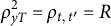
Comparing Equations (4.2) and (4.3), it is clear that the two approaches lead to the same reliability coefficient under CTT, that is,
$\rho _{yT}^2 = \rho _{t,t'} = R$
 . The variance partitioning approach is further generalized to study designs beyond CTT through the GT (Brennan & Kane, Reference Brennan and Kane1977a, Reference Brennan and Kane1977b; Cronbach, Reference Cronbach1972),Footnote
10
while the correlation approach keeps the same name. To underscore that the correlation and variance partitioning approach are two sides of the same coin, Bartko (Reference Bartko1966) stated that a reliability coefficient, when defined as a ratio of variances estimated through a linear model, is only valid when it can be interpreted as a form of correlation coefficient. This interpretation ensures that the reliability reflects the degree of similarity between repeated measurements rather than being a purely statistical artifact. However, we have shown that both approaches do not always lead to the same reliability coefficients in the context of multilevel data structures (Lin et al., Reference Lin, Tuerlinckx and Vanbelle2025).
4.2 Reliability in ILD: Challenges
Extending the concept of single-item reliability to ILD is not straightforward for several reasons. First, in CTT or GT as in multilevel reliability studies, the true score is assumed to be a stable attribute of an individual, constant over time or across different measurement occasions (Cranford et al., Reference Cranford, Shrout, Iida, Rafaeli, Yip and Bolger2006; Nezlek, Reference Nezlek2017; Shrout & Lane, Reference Shrout, Lane, Mehl and Conner2012a). In contrast, in ILD, the true score of individuals may vary over time due to situational factors, temporal dynamics, or other influences. This within-person fluctuation in true scores is a key feature of ILD, and it often reflects meaningful patterns of change that researchers are interested in. Second, this within-person fluctuation also generates new opportunities, because it allows us to distinguish the within-person variance from the between-person variance. Third, intensive longitudinal studies often involve additional sources of variability (e.g., day effects) that cannot be accounted for in CTT. Therefore, the traditional framework or methods for multilevel reliability analysis may not adequately capture the complexity of ILD data, and new approaches are needed to define and estimate reliability in that context.
Reliability for (intensive) longitudinal data can be defined either using the correlation approach or the variance partitioning approach. For example, in the context of the single-item measures, Vangeneugden et al. (Reference Vangeneugden, Laenen, Geys, Renard and Molenberghs2004, Reference Vangeneugden, Laenen, Geys, Renard and Molenberghs2005) formulated reliability via the correlation approach, while Laenen et al. (Reference Laenen, Alonso and Molenberghs2007, Reference Laenen, Alonso, Molenberghs and Vangeneugden2009a, Reference Laenen, Alonso, Molenberghs and Vangeneugden2009b) utilized the variance partitioning approach under the LMM framework. However, these earlier works did not explicitly distinguish reliability across different hierarchical levels, which is crucial for modern ILD studies. Notably, other studies have successfully employed the variance partitioning approach to define reliability in intensive longitudinal designs (see Leertouwer et al., Reference Leertouwer, Keijsers, van Roekel and Schuurman2025, for a comprehensive guide).Footnote 11 For instance, Schuurman and Hamaker (Reference Schuurman and Hamaker2019) and Schuurman et al. (Reference Schuurman, Houtveen and Hamaker2015) defined single-item reliability at both the between- and within-person levels within the multilevel measurement error autoregressive (ML-MEAR) model. However, their framework primarily considered a single AR(1) process across time within a two-level structure (e.g., repeated measurements nested within persons). While their model could theoretically be extended to accommodate a three-level structure (i.e., moments nested within days nested within persons), their reliability definitions yield static point estimates that do not explicitly account for how reliability fluctuates or decays over varying temporal lags. Furthermore, Dejonckheere et al. (Reference Dejonckheere, Demeyer, Geusens, Piot, Tuerlinckx, Verdonck and Mestdagh2022) proposed a model-free approach utilizing specific immediate- and delayed-retest designs to empirically isolate measurement error variance, which is then plugged back into the classical reliability formula. While highly innovative, Dejonckheere et al.’s (Reference Dejonckheere, Demeyer, Geusens, Piot, Tuerlinckx, Verdonck and Mestdagh2022) approach requires a specialized data collection design that is absent in standard, pre-existing ILD datasets like ours.
To address these challenges and bridge the methodological gap, the present study focuses specifically on formalizing single-item test–retest reliability within a dynamic LMM framework (recall Equation (3.5)). Although the two approaches (correlation vs. variance partitioning) lead to the same reliability coefficients within CTT (and other simple situations), this is not necessarily the case for more complex data structures (Lin et al., Reference Lin, Tuerlinckx and Vanbelle2025). Therefore, safely interpreting reliability in ILD applications requires understanding how these two approaches might diverge mathematically under complex true-score structures. In the following, we will formally derive reliability coefficients based on the correlation approach first and on the variance partitioning approach. For ease of distinction, the notation
$\rho $
 will denote reliability defined through the correlation approach, while the notation R will correspond to the one constructed by the variance partitioning approach.
4.3 Correlation approach to reliability for LMM
The correlation approach has been used before to define reliability for longitudinal data and for multilevel data. Vangeneugden et al. (Reference Vangeneugden, Laenen, Geys, Renard and Molenberghs2004, Reference Vangeneugden, Laenen, Geys, Renard and Molenberghs2005) proposed a general formula for reliability in longitudinal data using the correlation approach in the two-level LMM with one serial process, but they did not discuss how to distinguish the reliability at different hierarchical levels. On the other hand, Lin et al. (Reference Lin, Tuerlinckx and Vanbelle2025) further defined reliability coefficients for multilevel data at the different hierarchical levels, that is, between-person reliability and within-person reliability, but they did not consider any serial process. Thus, in this section, we will define reliability coefficients for a three-level model with serial correlation at two different time scales (day and moment).
4.3.1 Between-person reliability
Following the correlation approach (Lin et al., Reference Lin, Tuerlinckx and Vanbelle2025; Vangeneugden et al., Reference Vangeneugden, Laenen, Geys, Renard and Molenberghs2004, Reference Vangeneugden, Laenen, Geys, Renard and Molenberghs2005), the between-person test–retest reliability
$\rho ^{\text {B}}$
 is defined as the correlation between two measurements
$y_{ijk}$
 and
$y_{ij'k'}$
 of the same person i at two moments k and
$k'$
 on days j and
$j'$
 across the population. For conciseness, we define the time differences
$\Delta _{jj'} = |j-j'|$
 and
$\Delta _{kk'} = |k-k'|$
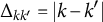 . Based on our three-level LMM model with two AR(1) processes (Equation (3.4)), the general formula for this correlation is (the full derivation is provided in Appendix A)

where the superscript
$\text {B}$
 indicates the between-person level and
$\delta _{jj'}$
 is the Kronecker delta equal to
$1$
 only if two moment measures are taken on the same day (i.e.,
$j=j'$
 ) and equal to 0 otherwise. The within-day serial correlation process does not play a role if the two moments considered are from different days
$j \neq j'$
 . Thus,
$\delta _{jj'}$
 determines whether
$\sigma _d^2$
 and
$\tau _m^2\phi _m^{\Delta _{kk'}}$
 appear in the numerator. Furthermore,
$\Delta _{jj'}$
 and
$\Delta _{kk'}$
 play vital roles in regulating the influence of the autoregressive effects
$\phi _d$
 and
$\phi _m$
 . Note that the two measurements
$y_{ijk}$
 and
$y_{ij'k'}$
 are not necessarily parallel (or tau-equivalent) in the CTT sense, because they may have different true scores due to the presence of within-person dynamic patterns. However,
$\rho ^{\text {B}}(\Delta _{jj'}, \Delta _{kk'})$
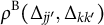 is still reflecting a crucial aspect of reliability: the agreement between two measurements across the population. Next, we will discuss several specific cases of the general formula.
Between-person moment-to-moment reliability: Suppose that researchers are interested in the between-person reliability across different moments (e.g., morning vs. afternoon) within a day, that is, the agreement of the measurements at two different moments
$k \neq k'$
 within the same day j across the population. Because
$\delta _{jj}=1$
 and
$\Delta _{jj'}=0$
 , the between-person moment-to-moment reliability coefficient of Equation (4.4) simplifies to

where the subscript
$\text {M}$
 indicates moment-to-moment. This reliability is a function of the time lag between the two moments
$\Delta _{kk'}$
 : The reliability decreases as
$\Delta _{kk'}$
 increases, because the two moments are more separated in time and thus the correlation between them is lower.
It might initially appear counterintuitive that day-related variances
$(\sigma _d^2$
 and
$\tau _d^2$
 ) persist in the numerator when computing moment-to-moment reliability. This occurs because assessing reliability between two moments strictly on the same day
$(j=j'$
 ) means these two measurements inherently share the exact same daily environmental characteristics and structural trajectory. Therefore, without conditioning on a specific fixed day, this shared daily variability fundamentally contributes as systematic variance, enhancing their overall similarity.
Between-person day-to-day reliability: Similarly, if researchers are interested in the reliability across different days (such that
$\Delta _{jj'}> 0$
 and
$\delta _{jj'}=0$
 ) across the population, the between-person day-to-day reliability coefficient is

where the subscript
$\text {D}$
 indicates day-to-day. In this case, k and
$k'$
 can be either the same or different, but because the measurements are located on different days (
$j \neq j'$
 ), they are disconnected by the moment-level AR trajectory. As a result, the decayed moment-level covariance
$\tau _m^2\phi _m^{\Delta _{kk'}}$
 drops out of the numerator. Similarly, because they are sampled from different days, they no longer share the same day effect
$d_{ij}$
 ; hence, the day variance
$\sigma _d^2$
 also vanishes from the numerator. Nevertheless, the day-level autoregressive component
$\tau _d^2\phi _d^{\Delta _{jj'}}$
 remains, reflecting that the two measurements are still systematically bound by the overarching day-level AR trajectory. The day-to-day reliability thus functions exclusively via the lag between days
$\Delta _{jj'}$
 , continuously decreasing as
$\Delta _{jj'}$
 increases.
Both Equations (4.5) and (4.6) reflect the reliability based on a single observation at different time points. However, in practice, researchers often use the average of multiple observations to represent a more stable score for a specific period. For example, researchers may use the average of moments within a day to represent the daily score for further analysis. When this is the case, they are wondering about the reliability of the composite score
$\bar {y}_{ij\cdot } = \frac {1}{M}\sum _{k=1}^M y_{ijk}$
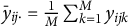 . Thus, there is another form of day-to-day reliability based on the average of moments within a day. In this case, the day-to-day reliability coefficient becomes

where the subscript
$\overline {\text {D}}$
 indicates the reliability for day-to-day based on the average of moments. Compared to Equation (4.6), the moment-level variance components
$\tau _m^2$
 and
$\sigma _{\varepsilon }^2$
 are now divided by M in the denominator because of the averaging operation, which leads to a smaller denominator and thus a larger result. This makes sense because the average of several measurements is at least as reliable as a single measurement.
Between-person stability and instantaneity: As can be seen in Equations (4.5) and (4.6), the temporal autocorrelation (decaying across time lags) between two measurements is an important component of the aforementioned reliability coefficients. Because of the presence of serial correlation and time lag in the reliability coefficients, it fits well in the distinction between long-term stability and short-term instantaneity, depending on the time lag, as defined by Boyle et al. (Reference Boyle, Stankov, Cattell, Saklofske and Zeidner1995), Cattell (Reference Cattell1964), and Revelle and Condon (Reference Revelle and Condon2019). Stability considers distant time points to evaluate the reliability over the whole measurement period or a further longer period, while instantaneity Footnote 12 considers two close time points to evaluate reliability immediately or in a short period.Footnote 13
Conceptually, we defined stability and instantaneity as the two extremes of a time lag spectrum in intensive longitudinal studies. Stability represents a test–retest correlation (Equation (4.4) or (4.6)) when the time lag is very large such that the influence of the autoregressive effect
$\phi _d$
 (and also
$\phi _m$
 ) completely disappears, or when, mathematically speaking, the time lag goes to infinity, that is,
$\phi _d^{\Delta _{jj'}} \to 0$
 as
$\Delta _{jj'} \to \infty $
 . As a result, the between-person stability coefficient is defined as

where the subscript
$\infty $
 indicates stability. This coefficient can be alternatively defined as the correlation between the current measurement
$y_{ijk}$
 and a hypothetical very distant future measurement
$y_{i\infty \infty }$
 from the same person i and then across the whole population, that is,
$\rho _{\infty }^{\text {B}} = \operatorname {\mathrm {Cor}}(y_{ijk}, y_{i\infty \infty })$
 . The numerator only consists of the between-person variance component
$\sigma _s^2$
 . All other sources of variance only appear in the denominator. This coefficient measures the degree to which individuals maintain their relative standing on the measured construct over an extended period, regardless of the specific time interval between assessments. Although the time lag to define stability is, in principle, infinitely long, for a substantive interpretation, it makes sense to think about it as “a very long time period in the context of the study.” Or stated differently, the time lag at which the autocorrelation has effectively vanished. To assess the stability of personality items, we may think of a period of several years. In contrast, if we are measuring mood, a very long time period can be as short as weeks.
On the contrary, instantaneity is defined as the test–retest reliability (Equation (4.4) or (4.5)) when the time lag between two measurements is very short such that the influence of the autoregressive effect is maximal, or mathematically speaking, the time lag goes to zero, that is,
$\phi _m^{\Delta _{kk'}} \to 1$
 as
$\Delta _{kk'} \to 0$
 . Thus, the between-person instantaneity coefficient is defined as

where the subscript
$0$
 indicates instantaneity. This coefficient can be alternatively defined as the correlation between the current measurement
$y_{ijk}$
 and a hypothetical parallel measurement
$y^{\prime }_{ijk}$
 from the same person i on the same day j at the same moment k, the only difference between the two measurements being the realized measurement error. Thus,
$\rho _{0}^{\text {B}} = \operatorname {\mathrm {Cor}}(y_{ijk}, y^{\prime }_{ijk})$
 . It shows that all variance components except the measurement error variance
$\sigma _{\varepsilon }^2$
 appear in the numerator. This coefficient quantifies the extent to which individuals maintain their relative standing on the measured construct over a very short period (as defined within the context of the study).
4.3.2 Within-person reliability
Within-person reliability focuses on the structural similarity of measurements within the same person instead of across the population of persons. We start again with a general formula for the within-person reliability coefficient
$\rho ^{\text {W}}$
 , defined as the correlation between two measurements
$y_{ijk}$
 and
$y_{ij'k'}$
 for a specific arbitrary person i (the full derivation is provided in Appendix A):

where the superscript
$\text {W}$
 indicates the within-person level. As before in Equation (4.4), the general formula is a function of the time lags
$\Delta _{jj'}$
 and
$\Delta _{kk'}$
 . However, unlike the between-person reliability, the person variance
$\sigma _s^2$
 disappears from both numerator and denominator because we consider a specific person i.
Again, moving across several time lags, we can define the within-person instantaneity, moment-to-moment reliability, and day-to-day reliability for single and average scores as follows:


All within-person reliability coefficients are derived from the conditional correlations, which result in formulas from which the person variance
$\sigma _s^2$
 is removed. Note that the within-person stability is undefined because it only makes sense for individual differences.
4.4 Variance partitioning approach to reliability for LMM
Reliability coefficients in the context of longitudinal data can also be defined based on the variance partitioning approach (Laenen et al., Reference Laenen, Alonso and Molenberghs2007; Laenen et al., Reference Laenen, Alonso, Molenberghs and Vangeneugden2009a, Reference Laenen, Alonso, Molenberghs and Vangeneugden2009b; Schuurman & Hamaker, Reference Schuurman and Hamaker2019; Schuurman et al., Reference Schuurman, Houtveen and Hamaker2015). There are two distinct (between-person) reliability coefficients worth noticing,
$R_{\text {T}}$
 (Laenen et al., Reference Laenen, Alonso and Molenberghs2007) and
$R_{\Lambda }$
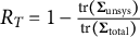
 (Laenen et al., Reference Laenen, Alonso, Molenberghs and Vangeneugden2009b). Both reliability coefficients are defined in a similar form as Equation (4.2), but in a matrix version:

where
$\boldsymbol {\Sigma }_{\text {unsys}}$
 is the unsystematic part of the total covariance matrix
$\boldsymbol {\Sigma }_{\text {total}}$
 and
$f(\cdot )$
 is a function, which can be either the trace for
$R_T = 1 - \frac {\operatorname {\mathrm {tr}}(\boldsymbol {\Sigma }_{\text {unsys}})}{\operatorname {\mathrm {tr}}(\boldsymbol {\Sigma }_{\text {total}})}$
 (Laenen et al., Reference Laenen, Alonso and Molenberghs2007) or the determinant for
$R_\Lambda = 1 - \frac {|\boldsymbol {\Sigma }_{\text {unsys}}|}{|\boldsymbol {\Sigma }_{\text {total}}|}$
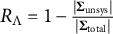 (Laenen et al., Reference Laenen, Alonso, Molenberghs and Vangeneugden2009b), to summarize the covariance matrix into a scalar.
For both cases (i.e.,
$R_T$
 and
$R_\Lambda $
 ), an important consideration is how to partition the variance components into a systematic and an unsystematic part. This classification depends on the research question. For example, Laenen et al. (Reference Laenen, Alonso and Molenberghs2007, Reference Laenen, Alonso, Molenberghs and Vangeneugden2009a, Reference Laenen, Alonso, Molenberghs and Vangeneugden2009b) argue that, based on their model of interest,Footnote
14
the systematic part should only include the stable individual differences, that is, the person-related covariance matrix, while the unsystematic part should include all other variance components, including the serial covariance matrix and measurement error covariance matrix. However, this partition is not absolute. In some ILD studies, temporal dynamics, such as daily or momentary fluctuations captured by AR(1) processes, represent meaningful, structured patterns and could therefore be considered as systematic variance. For example, if the research scope is restricted to daily trends (e.g., daily blood pressure level), then the day effect as well as the day-level serial effect should be considered as part of the systematic variance, while the moment-level serial effect should be treated as unsystematic variance. Conversely, if the research focus is on the dynamic process itself (e.g., momentary mood regulation or emotional inertia), then the moment serial effect should be considered as part of the systematic variance.
Depending on three different partitions of the variance components, we can construct three subtypes of
$R_{\text {T}}$
 Footnote
15
based on our three-level LMM with two AR(1) processes (Equation (3.5)). As before, we distinguish between-person reliability and within-person reliability for each subtype. This leads to five reliability coefficients based on variance partitioning. In the next section, we will explain how these coefficients are related.
4.4.1 Between-person reliability
As shown in Equation (3.6), the total variance matrix of the observation
$\boldsymbol {V}$
 is decomposed into five variance components: the person-related covariance matrix
$\boldsymbol {\Sigma }_S$
 , the day-related covariance matrices
$(\boldsymbol {\Sigma }_D$
 and
$\boldsymbol {\Sigma }_\nu $
 ), moment-related covariance matrix
$\boldsymbol {\Sigma }_\omega $
 , and measurement error covariance matrix
$\boldsymbol {\Sigma }_E$
 .
Reliability for momentary scores: If the momentary score is the measurement of interest, then the question is to which extent this score can be differentiated from other momentary scores (from the same person or from other persons). In this case, all variance components related to person, day, and moment are considered systematic. Only random measurement error
$(\boldsymbol {\Sigma }_E$
 ) is treated as unsystematic. The reliability is defined as

where the subscript
$\text {TM}$
 indicates reliability based on the trace for the momentary score, and the superscript
$\text {B}$
 indicates the between-person level.
$R_{\text {TM}}^{\text {B}}$
 reflects the belief that even though momentary states fluctuate, these fluctuations are part of a meaningful dynamic process. Especially in objective physiological measures, such as heart rate or cortisol levels, the moment-to-moment fluctuations can be systematic and informative about an individual’s current state.
The coefficient
$R_{\text {TM}}^{\text {B}}$
 is equivalent to the between-person instantaneity coefficient defined by the correlation approach:
$R_{\text {TM}}^{\text {B}} = \rho _{0}^{\text {B}}$
 . This equivalence tells that both reliability coefficients can be interpreted in two different ways: (1) to which extent can the momentary score be used to differentiate between individuals across the population (based on the variance partitioning approach) and (2) the level of agreement between individual momentary scores over an extremely short period of time (based on the correlation approach). This dual interpretation highlights the multifaceted nature of reliability in ILD.
Reliability of daily scores: When the target of measurement is the score at the day level, the moment-to-moment fluctuations within a day are considered unsystematic noise. In this case, the systematic variance includes only the person- and day-level components
$(\boldsymbol {\Sigma }_S, \boldsymbol {\Sigma }_D, \boldsymbol {\Sigma }_\nu $
 ), while the unsystematic variance includes the moment-level serial process
$(\boldsymbol {\Sigma }_\omega $
 ) and measurement error
$(\boldsymbol {\Sigma }_E$
 ). The reliability is defined as

where the subscript
$\text {TD}$
 indicates reliability for the daily score.
The coefficient
$R_{\text {TD}}^{\text {B}}$
 is equivalent to the between-person moment-to-moment reliability
$\rho _{\text {M}}^{\text {B}}(\Delta _{kk'})$
 for a large within-day time lag
$\Delta _{kk'}$
 (such that the moment-level autoregressive effect
$\phi _m$
 vanishes). Consequently, this reliability coefficient quantifies: (1) to which extent the daily score can be used to differentiate between individuals across the population (based on the variance partitioning approach) and (2) the level of agreement between the observed scores over a long interval within the same day (based on the correlation approach). In other words,
$R_{\text {TD}}^{\text {B}}$
 reflects within-day stability.
Reliability of person (trait) scores: Lastly, if the goal is to measure a stable, person-level trait, all sources of within-person variance (daily fluctuations, momentary dynamics, and measurement error) can be considered unsystematic. The systematic variance is confined to the stable between-person component
$(\boldsymbol {\Sigma }_S$
 ). This perspective is common when researchers believe temporal dynamics are nuisance factors rather than meaningful signals. The reliability is defined as

where the subscript
$\text {TP}$
 indicates reliability of the personal trait-like score. This reliability coefficient should be considered when any day-to-day and moment-to-moment fluctuations, together with their serial correlation, are considered as error and do not truly explain the difference in individual traits. This is reasonable, for example, when considering that serial patterns arise from carry-over effects, such as memory effects or practice effects, which can occur in studies involving self-report measurements.
This coefficient is equivalent to the between-person stability coefficient
$R_{\text {TP}}^{\text {B}} = \rho _{\infty }^{\text {B}}$
 and indicates that this reliability coefficient quantifies: (1) to which extent the trait-like score can differentiate between individuals across the population (based on the variance partitioning approach) and (2) the level of agreement between trait-like scores within individuals over an extended period (based on the correlation approach).
4.4.2 Within-person reliability
The same variance partitioning logic can be applied at the within-person level. In this case, however, not the total variance
$\boldsymbol {V}$
 will be partitioned, but the individual-level variance
$\boldsymbol {V}_i$
 (see Equation (3.7)).
$\boldsymbol {V}_i$
 is composed of four parts: the day-related covariance matrices (
$\boldsymbol {\Sigma }_D$
 and
$\boldsymbol {\Sigma }_\nu $
 ), the moment-related covariance matrix
$\boldsymbol {\Sigma }_\omega $
 , and the measurement error covariance matrix
$\boldsymbol {\Sigma }_E$
 . Depending on the measurement of interest (e.g., a momentary score or a daily score), there are two subtypes of
$R_{\text {T}}$
 at the within-person level:


where the superscript
$\text {W}$
 indicates the within-person level.
$R_{\text {TM}}^{\text {W}}$
 focuses on the momentary score within a person, so the unsystematic part only includes the measurement error covariance matrix
$\boldsymbol {\Sigma }_E$
 . This coefficient is equivalent to the within-person instantaneity coefficient
$R_{\text {TM}}^{\text {W}} = \rho _{0}^{\text {W}}$
 .
$R_{\text {TD}}^{\text {W}}$
 , focusing on the daily score within a person, considers both the moment-related covariance matrix
$\boldsymbol {\Sigma }_\omega $
 and measurement error covariance matrix
$\boldsymbol {\Sigma }_E$
 as the unsystematic part. This coefficient is equivalent to the within-person moment-to-moment reliability
$\rho _{\text {M}}^{\text {W}}(\Delta _{kk'})$
 when the time lag
$\Delta _{kk'}$
 within a day is large enough such that the moment-level autoregressive effect
$\phi _m$
 diminishes.
Both coefficients
$R_{\text {TM}}^{\text {W}}$
 and
$R_{\text {TD}}^{\text {W}}$
 quantify: (1) to which extent the measurement of interest (at the moment or day level) can differentiate between different time points within the same person from the variance partitioning viewpoint and (2) the level of agreement between target scores (momentary or daily score) within a person over a short period from the correlation viewpoint.
A further step could be to define
$R_{\text {TP}}^{\text {W}}$
 as the reliability coefficient for the within-person trait-like score. However, as the explanation in words already suggests, this coefficient cannot be determined. The reason is obvious: the person-level variance
$\sigma _s^2$
 is removed in both numerator and denominator when we condition on a specific person i. Consequently, there is no systematic variance component left in the numerator if we consider all other variance components as the unsystematic part. Similarly, we could not define the within-person stability coefficient using the correlation approach.
To summarize, we collect the aforementioned reliability coefficients for the three-level LMM with two AR(1) processes in a single row (“M1”) in Table 1 for the between-person level and in Table 2 for the within-person level, respectively. From left to right, the time lag of interest widens, ranging from instantaneity to moment-to-moment fluctuations to day-to-day fluctuations to stability. It can be seen that the reliability coefficients defined by the variance partitioning approach are equivalent to those defined by the correlation approach under some conditions. This equivalence highlights that the correlation and variance partitioning approaches represent two distinct perspectives on the same underlying concept of reliability, which can, in some cases, yield identical results.
Comparison of between-person reliability coefficients across four models

Table 1 Long description
The table consists of four rows representing models M 1 through M 4 and five columns for time spans: Instantaneity, Moment-to-moment (two sub-columns), Day-to-day, and Stability.
* Row 1 (M 1: Three-level L M M with two A R 1):
- Instantaneity: rho sub 0 super B equals R sub T M super B equals the fraction with numerator sigma sub s squared plus sigma sub d squared plus tau sub d squared plus tau sub m squared all over denominator sigma sub s squared plus sigma sub d squared plus tau sub d squared plus tau sub m squared plus sigma sub varepsilon squared.
- Moment-to-moment (first): rho sub M super B (Delta sub k k prime) equals the fraction with numerator sigma sub s squared plus sigma sub d squared plus tau sub d squared plus tau sub m phi sub m to the Delta sub k k prime power all over the same denominator as Instantaneity.
- Moment-to-moment (second): rho sub M super B (Delta sub k k prime super plus) equals R sub T D super B equals the fraction with numerator sigma sub s squared plus sigma sub d squared plus tau sub d squared all over the same denominator.
- Day-to-day: rho sub D super B (Delta sub j j prime) equals the fraction with numerator sigma sub s squared plus tau sub d phi sub d to the Delta sub j j prime power all over the same denominator.
- Stability: rho sub infinity super B equals R sub T P super B equals the fraction with numerator sigma sub s squared all over the same denominator.
* Row 2 (M 2: Three-level L M M):
- Instantaneity to Moment-to-moment: rho sub 0 super B equals rho sub M super B equals R sub T M super B equals R sub T D super B equals the fraction with numerator sigma sub s squared plus sigma sub d squared all over denominator sigma sub s squared plus sigma sub d squared plus sigma sub varepsilon squared.
- Day-to-day to Stability: rho sub D super B equals rho sub infinity super B equals R sub T P super B equals the fraction with numerator sigma sub s squared all over denominator sigma sub s squared plus sigma sub d squared plus sigma sub varepsilon squared.
* Row 3 (M 3: Two-level L M M with one A R 1):
- Instantaneity: rho sub 0 super B equals R sub T M super B equals the fraction with numerator sigma sub s squared plus tau sub t squared all over denominator sigma sub s squared plus tau sub t squared plus sigma sub varepsilon squared.
- Moment-to-moment to Day-to-day: rho sub T super B (Delta sub t t prime) equals the fraction with numerator sigma sub s squared plus tau sub t squared phi to the Delta sub t t prime power all over the same denominator as M 3 Instantaneity.
- Stability: rho sub infinity super B equals R sub T P super B equals the fraction with numerator sigma sub s squared all over the same denominator.
* Row 4 (M 4: Two-level L M M equivalent to C T T):
- All time spans: rho equals R equals the fraction with numerator sigma sub s squared all over denominator sigma sub s squared plus sigma sub varepsilon squared.
Note:
$\rho $
 = reliability based on the correlation approach; R = reliability based on the variance partitioning approach; superscripts
$\text {B}$
 = between-person level and
$\text {W}$
 = within-person level; subscripts
$0$
 = instantaneity,
$\text {M}$
 = moment-to-moment;
$\text {D}$
 = day-to-day,
$\text {T}$
 = test–retest,
$\infty $
 = stability,
$\text {TM}$
 = momentary scores,
$\text {TD}$
 = daily score,
$\text {TP}$
 = personal trait scores;
$\Delta _{kk'}$
 = time lag between moments,
$\Delta _{kk'}^+$
 = a large time lag between moments such that the moment-level autoregressive effect
$\phi _m$
 diminishes,
$\Delta _{jj'}$
 = time lag between days, and
$\Delta _t$
 = time lag between moments/measurements.
4.5 Comparing reliability coefficients for different models
To better understand the relationships among various reliability coefficients, we consider four related models with varying degrees of complexity, where simpler models are nested within the more complex ones. The four models for comparison are:
-
M1: a three-level LMM with two AR(1) processes as defined before in Equation (3.4);
-
M2: a three-level LMM but without any serially correlated processes: $y_{ijk} = \beta + s_i + d_{ij} + {\varepsilon }_{ijk}$
 ;
-
M3: a two-level LMM with one AR(1) process at the moment level: $y_{it} = \beta + s_i + \omega _{it} + {\varepsilon }_{it}$
; -
M4: a two-level LMM without any serial process: $y_{it} = \beta + s_i + {\varepsilon }_{it}$
.



Models M1 and M2 assume a three-level data structure (moments nested within days, and days nested within persons), while models M3 and M4 assume a two-level structure by ignoring one level (moments nested within persons). For models M3 and M4, we have combined the two time indices j and k into a single time index t, where
$t = 1, \dots , D \times M$
 . Thus, the time lag between any pair of measurements is denoted as
$\Delta _t = |t - t'|$
 . In addition, model M3 is also the main model (but without person covariates) discussed in Laenen et al. (Reference Laenen, Alonso and Molenberghs2007, Reference Laenen, Alonso, Molenberghs and Vangeneugden2009b) and Vangeneugden et al. (Reference Vangeneugden, Laenen, Geys, Renard and Molenberghs2004, Reference Vangeneugden, Laenen, Geys, Renard and Molenberghs2005). Model M4 is equivalent to the traditional CTT model where the true score
$T_i$
 is defined as
$T_i = \beta + s_i$
 .
Tables 1 and 2 summarize the reliability coefficients for the between-person and within-person levels, respectively. There are some key findings that can be derived from these two tables. First, comparing models M1 and M3 to M2 and M4, respectively, the difference is the inclusion of serial correlation. The models with serial correlation have more comprehensive reliability coefficients compared to those which do not account for any serial correlation. These permit the distinction between instantaneity, moment-to-moment, day-to-day, and stability. Second, because of the three-level structure in model M2, we can still distinguish between the moment-to-moment reliability
$\rho _{M}$
 and day-to-day reliability
$\rho _{D}$
 . Nevertheless, both reliabilities are constant because there is no serial correlation in the model. Therefore, regardless of which pair of measurements is selected and used in the correlation, the reliability remains the same. For example, let us focus on the correlation between the measurement of person i on day j and moment k,
$y_{ijk}$
 , and correlate this with the measurement one moment later (i.e.,
$y_{ij,k+1}$
 ) or two moments later (i.e.,
$y_{ij,k+2}$
 ). It turns out that in model M2,
$\rho _{M}(\Delta _{kk'} = 1) = \operatorname {\mathrm {Cor}}(y_{ijk}, y_{ij,k+1}) = \frac {\sigma _s^2 + \sigma _d^2}{\sigma _s^2 + \sigma _d^2 + \sigma _{\varepsilon }^2} = \operatorname {\mathrm {Cor}}(y_{ijk}, y_{ij,k+2})=\rho _{M}(\Delta _{kk'} = 2) $
 . Third (and as said above), some reliabilities related to stable traits cannot be defined (or always be 0) for the within-person level (Table 2). This is a necessary consequence of conditioning on the person, which removes the between-person variance that defines these coefficients.
In addition, it is theoretically illuminating to demonstrate how the reliability coefficients derived from our simplified models seamlessly connect to existing reliability formulations in the literature. For the three-level model without autocorrelation (M2), the data structure conceptually mirrors the three-level GT framework often used for multiple-item ESM data when items are modeled as nested within time pointsFootnote
16
(in contrast to our moments nested within days at the lower levels), which are in turn nested within persons (e.g., Nezlek, Reference Nezlek2017; Nezlek & Gable, Reference Nezlek and Gable2001; Shrout & Lane, Reference Shrout, Lane, Mehl and Conner2012a). If we constrain their GT framework to evaluate the reliability of a single item measured at a single time point, the between-person reliability formula (e.g., Equation 10 in Shrout & Lane, Reference Shrout, Lane, Mehl and Conner2012a) is mathematically identical to our between-person reliability without autocorrelation
$(\rho _\infty ^{\text {B}}$
 from Table 1). Similarly, their within-person reliability formula (e.g., Equation 11 in Shrout & Lane, Reference Shrout, Lane, Mehl and Conner2012a) shares the exact same form as our within-person reliability
$(\rho _0^{\text {W}}$
 from Table 2).
Comparison of within-person reliability coefficients across four models
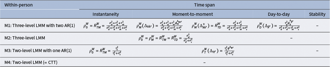
Table 2 Long description
The table is organized into six columns. The first column lists the models, and the remaining five columns are grouped under the heading Time span, which includes Instantaneity, Moment-to-moment (split into two sub-columns), Day-to-day, and Stability.
* Row 1: M 1: Three-level L M M with two A R (1).
- Instantaneity: rho sub 0 super W = R sub T M super W = (sigma sub d squared + tau sub d squared + tau sub m squared) all over (sigma sub d squared + tau sub d squared + tau sub m squared + sigma sub varepsilon squared).
- Moment-to-moment (first sub-column): rho sub M super W (Delta sub k k prime) = (sigma sub d squared + tau sub d squared + tau sub m squared phi sub m super Delta sub k k prime) all over (sigma sub d squared + tau sub d squared + tau sub m squared + sigma sub varepsilon squared).
- Moment-to-moment (second sub-column): rho sub M super W (Delta sub k k prime super +) = R sub T D super W = (sigma sub d squared + tau sub d squared) all over (sigma sub d squared + tau sub d squared + tau sub m squared + sigma sub varepsilon squared).
- Day-to-day: rho sub D super W (Delta sub j j prime) = (tau sub d squared phi sub d super Delta sub j j prime) all over (sigma sub d squared + tau sub d squared + tau sub m squared + sigma sub varepsilon squared).
- Stability: No data.
* Row 2: M 2: Three-level L M M.
- Instantaneity through Moment-to-moment: rho sub 0 super W = rho sub M super W = R sub T M super W = R sub T D super W = sigma sub d squared all over (sigma sub d squared + sigma sub varepsilon squared).
- Day-to-day and Stability: No data.
* Row 3: M 3: Two-level L M M with one A R (1).
- Instantaneity: rho sub 0 super W = R sub T M super W = tau sub t squared all over (tau sub t squared + sigma sub varepsilon squared).
- Moment-to-moment through Day-to-day: rho sub T super W (Delta sub t t prime) = (tau sub t squared phi super Delta sub t t prime) all over (tau sub t squared + sigma sub varepsilon squared).
- Stability: No data.
* Row 4: M 4: Two-level L M M (equals C T T). No data provided for any time span.
Note: Same notations in Table 1.
Likewise, the two-level model with a single AR(1) process (M3) corresponds closely to the ML-MEAR model proposed by Schuurman and Hamaker (Reference Schuurman and Hamaker2019), albeit they formulate it using a state-space representation.Footnote
17
Under the assumption of constant model parameters, the between-person reliability in the ML-MEAR framework (Equation 7 in Schuurman & Hamaker, Reference Schuurman and Hamaker2019) equals our
$\rho _\infty ^{\text {B}}$
 derived under M3. Analogously, their within-person reliability (Equation 9 in Schuurman & Hamaker, Reference Schuurman and Hamaker2019) is equivalent to our
$\rho _0^{\text {W}}$
 .
Finally, the traditional reliability in CTT (model M4) can be seen as the most basic special case for the more complex models (M1, M2, and M3) when we ignore the serial correlation and multilevel data structure. Thus, the traditional reliability (Equation (4.1)) is always a constant and cannot capture the rich and dynamic nature of ILD.
It is worth noting that while it is theoretically possible to compute reliability coefficients from simplified models (e.g., ignoring a level of nesting or assuming zero autocorrelation), we strongly advise against choosing a model solely for the sake of obtaining a “better” or specific reliability value. Reliability estimates are only meaningful when derived from a model that adequately represents the data bonding structure. For instance, applying a two-level model to three-level data (ignoring day-level clustering) or neglecting substantial serial correlation may result in biased variance component estimates, which in turn propagate into biased reliability coefficients. Therefore, the selection of the reliability formula (M1–M4) should follow the design of the study and the underlying data structure.
5 Illustration using the Exam Results Study
In this section, we apply our developed reliability coefficients to the Exam Results Study (Kalokerinos et al., Reference Kalokerinos, Erbas, Ceulemans and Kuppens2019). As indicated in the introductory section on the Exam Results Study, there are three distinct questions of interest regarding reliability, each answered by specific coefficients derived from our models: (1) To what extent does the single-item measure reflect a stable, trait-like tendency that distinguishes persons from one another? This is addressed by the stability coefficient (e.g.,
$\rho _\infty ^{\text {B}} = R_{\text {TP}}^{\text {B}}$
 ). (2) To what extent would repeating the measurement at the exact same given moment yield a similar result? This is addressed by the instantaneity coefficients at both the between- and within-person levels (e.g.,
$\rho _0^{\text {B}} = R_{\text {TM}}^{\text {B}}$
 and
$\rho _0^{\text {W}} = R_{\text {TM}}^{\text {W}}$
 ). Finally, (3) how does the agreement between measurements change across varying time intervals? This is addressed by evaluating the reliability functions over varying time lags (e.g.,
$\rho _{\text {M}}^{\text {B}}$
 ,
$\rho _{\text {D}}^{\text {B}}$
 ,
$\rho _{\text {M}}^{\text {W}}$
 , and
$\rho _{\text {D}}^{\text {W}}$
 ).
To investigate these questions, we apply the three-level model with autoregressive processes at two levels (Equation (3.4)) to analyze the single-item negative affect measurement. More information about the sample and the measurement procedure can be found in Section 2 and the original paper (Kalokerinos et al., Reference Kalokerinos, Erbas, Ceulemans and Kuppens2019). In the current analysis, all students have been included.
5.1 Methods
Model parameters and reliability coefficients were estimated using Bayesian inference for two reasons. First, the three-level model with two serially correlated processes is not a standard model that can be easily fit using non-Bayesian software. Second, we want to quantify the uncertainty of the reliability coefficients. Both objectives are easier to reach in a Bayesian inferential framework.
The fitting procedure is as follows: we started from a three-level LMM model without any AR(1) structure. Then, we added AR(1) structures to the moment level and day level sequentially if the MCMC sampler converged well and the parameters for the AR(1) process were significantly different from zero. We used R (version 4.5.0; R Core Team, 2025) with the cmdstanr package (version 0.9.0; Gabry et al., Reference Gabry, Češnovar, Johnson and Bronder2025) as an interface of Stan (version 2.36.0; Stan Development Team, 2025a, 2025b) to fit the model. Missing data were handled by setting them as unknown parameters to be estimated. We ran four MCMC chains with 64,000 iterations each, a thinning factor of 8, and considering the first 32,000 iterations as warm-up. The total number of post-warm-up draws across four chains was therefore 16,000.Footnote 18 The various reliability coefficients were derived afterward based on the posterior samples of the model parameters. The Stan code and R code for data processing, model fitting, and result visualization are available on the Open Science Framework (OSF) at https://osf.io/hnkuc. The original data for the Exam Results Study can be accessed from the EMOTE database or from the authors’ OSF repository.Footnote 19
5.2 Results
The posterior means, posterior standard deviations, and 95% highest density intervals (HDIs) of the posterior distribution of the key model parameters are summarized in Table 3. Convergence was achieved for all parameters for our proposed model M1 (Equation (3.4)), with R-hat
$(\hat {R}$
 ) values below 1.015 (Vehtari et al., Reference Vehtari, Gelman, Simpson, Carpenter and Bürkner2021) and a minimal effective sample size of 269.5 for the measurement error SD,
$\sigma _{\varepsilon }$
 . Trace plots and autocorrelation plots of the key parameters confirmed good mixing and convergence (see the results on OSF).
Posterior summary statistics for the parameters of the three-level model applied to the Exam Results Study

Table 3 Long description
The table consists of five columns: Parameter, Posterior mean (posterior S D), Posterior 95% H D I, R-hat, and E S S. It is divided into three thematic sections.
* Fixed effect section:
- beta (grand mean): 19.48 (1.26); H D I [17.04, 21.54]; R-hat 1.00; E S S 14,677.32.
* Autoregressive effect section:
- phi sub d (day level): 0.57 (0.08); H D I [0.46, 0.71]; R-hat 1.00; E S S 3,771.06.
- phi sub m (moment level): 0.45 (0.08); H D I [0.32, 0.58]; R-hat 1.01; E S S 297.65.
* Standard deviation section:
- sigma sub s (person random effect): 10.39 (1.60); H D I [7.95, 12.56]; R-hat 1.00; E S S 6,030.31.
- sigma sub d (day random effect): 1.49 (1.08); H D I [0.13, 3.55]; R-hat 1.00; E S S 3,104.66.
- tau sub d (stationary S D day): 11.17 (0.88); H D I [9.98, 12.69]; R-hat 1.00; E S S 6,313.74.
- tau sub m (stationary S D moment): 11.16 (0.84); H D I [9.96, 12.71]; R-hat 1.01; E S S 283.68.
- sigma sub epsilon (measurement error): 10.80 (1.04); H D I [8.82, 12.10]; R-hat 1.01; E S S 269.47.
Note:
$\hat {R}$
 : convergence diagnostic; ESS: effective sample size;
$\beta $
 : grand mean;
$\phi _d$
 and
$\phi _m$
 : autoregression effect of AR(1) process for day and moment levels;
$\sigma _s$
 ,
$\sigma _d$
 ,
$\sigma _{\varepsilon }$
 : SDs of person random effect, day random effect, and measurement error; and
$\tau _d$
 and
$\tau _m$
 : stationary SD of AR(1) process for day and moment levels.
The estimated between-person standard deviation
$\hat {\sigma }_s$
 equals 10.39, suggesting substantial variability in negative affect levels among individuals. The day-level standard deviation
$(\hat {\sigma }_d=1.49$
 ) is estimated to be relatively small, indicating that day-to-day fluctuations in negative affect are less pronounced as compared to between-person differences
$\hat {\sigma }_s$
 and the estimated measurement error
$\hat {\sigma }_{{\varepsilon }}=10.80$
 . This also means that there was only little variation between days, after accounting for carry-over effects. The measurement error quantifies the size of the average uncorrelated momentary deviations. Because there are no serial dependencies, it is a pure noise process. However, the day-to-day variation is also influenced by the serial correlation process, which has a stationary standard deviation of
$\hat {\tau }_d=11.17$
 . The stationary standard deviation of the moment-to-moment serial correlation process is of the same order of magnitude (i.e.,
$\hat {\tau }_m=11.16$
 ).
The relatively large magnitudes of the stationary standard deviations are partly due to the moderately sized autoregressive parameters, both for day-level
$(\hat {\phi }_d=0.57$
 ) and moment-level
$(\hat {\phi }_m=0.45$
 ). For both parameters, the posteriors are substantially larger than zero. However, the values of the day and moment autoregressive parameters are not directly comparable because they depend on time intervals with different units between assessments (1 day at the day level and around 1.2 hours at the moment level). This suggests considerable variability in negative affect within individuals over time.
Based on the estimated parameters and the formulas presented in this article, we can calculate all the reliability coefficients. In Figure 1, both the between-person (left panel) and within-person (right panel) reliability estimates are presented. In each plot, the x-axis represents the time lag between two assessments. The time lag ranges from 0 (for the instantaneity) across 10 moments
$(\Delta _{kk'} = 1, \dots , 9$
 ) and then across 9 days
$(\Delta _{jj'} = 1, \dots , 8$
 ), ending with a very large time lag (for the stability). The reliability estimates lie on the y-axis. In the plot, each dot represents the posterior mean of the reliability estimates, and the thick and thin vertical bars represent the 50% and 95% HDIs, respectively. These results are also given in Table B1 in Appendix B.
Between- (Panel (a)) and within-person (Panel (b)) reliability estimates for the single-item negative affect assessment in the Exam Results Study. In each panel, there are three (or two) gray vertical strips, corresponding to the instantaneity
$(\rho _{0} = R_{\text {TM}}$
 ), moment-to-moment long-term reliability
$(R_{\text {TD}}$
 ), and stability
$(\rho _{\infty } = R_{\text {TP}}$
 , only for between-person level). In between, we find the moment-to-moment reliabilities
$\rho _{\text {M}}$
 (for time lag
$\Delta _{kk'} = 1, \dots , 9$
 ) and day-to-day reliabilities
$\rho _{\text {D}}$
 (for time lag
$\Delta _{jj'} = 1, \dots , 8$
 ). All reliabilities are for the single negative affect item, but for comparison, the reliability of the average day score is added as well.

Figure 1 Long description
A two-panel dot plot with Panel a on the left titled Between-person level in blue and Panel b on the right titled Within-person level in red. Both panels share a y-axis labeled Value ranging from 0.0 to 1.0 and an x-axis labeled Reliability.
Panel a (Between-person):
- The legend indicates light blue circles for Single scores and dark blue squares for Averaged scores.
- A gray vertical strip at the far left contains rho sub 0 = R sub T M with a value near 0.75.
- Moving right, rho sub M (Delta k k prime = 1 to 9) shows a decaying trend from 0.65 down to 0.5.
- A second gray strip contains R sub T D with a value near 0.5.
- To the right, rho sub D (Delta j j prime = 1 to 8) shows two series. The Single score drops from 0.4 to 0.2, while the Averaged score starts higher at 0.7 and decays to 0.4.
- A final gray strip at the far right contains rho sub infinity = R sub T P with a value near 0.25.
Panel b (Within-person):
- The legend indicates light red circles for Single scores and dark red squares for Averaged scores.
- The first gray strip rho sub 0 = R sub T M shows a value near 0.7.
- rho sub M (Delta k k prime = 1 to 9) decays from 0.5 to 0.35.
- The second gray strip R sub T D shows a value near 0.35.
- rho sub D (Delta j j prime = 1 to 8) shows the Single score dropping from 0.2 to near 0, while the Averaged score starts at 0.5 and decays toward 0.
- Error bars representing confidence intervals are present for all data points, generally wider for the within-person estimates.
We can now address our three research questions using the reliability estimates presented in Figure 1. In short, these reliability coefficients indicate how well the single-item instrument can distinguish measurements across different time intervals: from very short intervals (nearly instantaneous), to short intervals (hours), to longer intervals (days), and ultimately very long intervals (reflecting stability).
To answer question (1), we quantify how well the single-item measure reflects a trait-like tendency that allows us to distinguish between persons. We look at the long-term between-person reliability, or stability
$R_{\text {TP}}^{\text {B}}$
 . As shown in panel (a) of Figure 1, this value is 0.23 (95% HDI [0.14, 0.31]). This low coefficient indicates that only 23% of the variance in a single measurement can be attributed to stable, trait-like differences between individuals. Consequently, the current design combined with a single-item measure has very limited utility for distinguishing people based on a stable negative affect level.
To answer question (2), we need to determine the extent to which repeating the measurement under the exact same conditions at a given moment would yield (dis)similar results. We refer to the instantaneous reliability coefficient. Between-person instantaneous reliability
$R_{\text {TM}}^{\text {B}}$
 = 0.76 (95% HDI [0.69,0.84]), suggesting that the measurements can effectively differentiate individuals’ current states at a specific moment. Concurrently, within-person instantaneous reliability
$R_{\text {TM}}^{\text {W}}$
 = 0.68 (95% HDI [0.60,0.79]), indicating that it reasonably captures a person’s momentary state.
Finally, to answer question (3), we quantify the degree of agreement of single-item measurements across time. This question can be separated into two parts: between-person reliability (see Figure 1a) and within-person reliability (see Figure 1b). At the between-person level, the instantaneous reliability initially drops steeply but then stabilizes around
$R_{\text {TD}}^{\text {B}}$
 = 0.50 (95% HDI [0.46,0.54]) after three time units
$(\Delta _{kk'} = 3$
 ), corresponding approximately to
$3.6 = 12 / 10 * (4 - 1)$
 hours. When considering longer time intervals, the between-person reliability is approximately 0.38 (95% HDI [0.33,0.43]) for one day and stabilizes after four days to 0.23 (the stability reliability). This shows that the negative affect scale is capable of distinguishing between persons only across time intervals as small as 1.2 hours. This is partially due to the low autocorrelation between the observations made at different moments and on different days, meaning that negative affects do not persist over time. Averaging observations over days increases reliability to allow the distinction between students when measurements are taken one day apart (
$\rho _{\overline {\text {D}}}^{\text {B}}(\Delta _{jj'} = 1)$
 =0.70, 95% HDI [0.65,0.74]) but decreases too much after two days. The primary trade-off of using average daily scores is the loss of the personal dynamic patterns within the day.
In contrast, at the within-person level, the instantaneous reliability quickly drops to stabilize around 0.35 (95% HDI [0.30,0.41]) after 3.6 hours within the same day. Day-to-day similarity is around 0.19 (95% HDI [0.14,0.17]) after one day lag, and rapidly decreases. This shows that, within a typical person, the negative affect does not persist in time. This pattern demonstrates that, for a typical individual, negative affect is highly dynamic and does not persist strongly over time, due to the combination of the small autoregressive effect and stationary day variance. The measurement is sensitive enough to capture momentary states, but these states are transient, highlighting the fluctuating nature of emotional experiences. Likewise, using average daily scores can increase reliability, but only to a limited extent.
6 Discussion
The main contribution of this article is to propose a general framework for single-item reliability for a common type of ILD (moments within days within persons). Starting from a three-level LMM with two AR(1) processes to account for the multilevel structure as well as the serial correlation structure, a family of reliability coefficients (both at the between-person and within-person level) can be derived and interpreted based on two different approaches: the correlation and variance partitioning approaches.
The correlation approach defines reliability at between- and within-person levels as a correlation (conditioned on a specific person at the within-person level) between two measurements taken at different time points, emphasizing the sheer degree of similarity between them. Specifically, we separate test–retest reliability into four types based on the time interval considered: instantaneity (extremely short-term,
$\rho _{0}$
 ), moment-to-moment
$(\rho _{\text {M}}$
 ), day-to-day
$(\rho _{\text {D}}$
 ), and stability (extremely long-term,
$\rho _{\infty }$
 ), reflecting the three-level structure of the ILD. This is crucial in the presence of ILD, as ignoring the serial correlation may lead to biased estimates of the variance components, which in turn result in misleading reliability estimates.
In contrast, the variance partitioning approach defines reliability as the proportion of total variance to the systematic variance (e.g., variance of the person’s true scores). It stresses the ability of the measurement instrument to distinguish the target of interest from measurement error. We further extended Laenen et al.’s (Reference Laenen, Alonso and Molenberghs2007) reliability
$R_{\text {T}}$
 into three subtypes: reliability of the momentary true scores
$(R_{\text {TM}}$
 ), daily true scores
$(R_{\text {TD}}$
 ), and person (trait) scores
$(R_{\text {TP}}$
 ). Each of them can be further defined at between- and within-person levels, with the exception of within-person reliability of the trait score
$(R_{\text {TP}}^{\text {W}}$
 ), which is undefined. We have elucidated the connections between the various coefficients. In addition, we showed how this family of coefficients is directly related to reliability coefficients arising from simpler models, most notably the CTT model.
Finally, our framework has been applied to the empirical Exam Results Study (Kalokerinos et al., Reference Kalokerinos, Erbas, Ceulemans and Kuppens2019). As expected, the test–retest reliability (based on the correlation interpretation) gradually decreased as the time lag increased, and the between-person reliability (ranging from 0.23 to 0.78) was uniformly higher than the within-person reliability (ranging from 0.01 to 0.68). Based on these results, we can conclude that after around 3.6 hours within a day, the between-subject agreement has reached its asymptote. In the same vein, the between-subject agreement of measurements taken about four days apart is close to that of the long-term stability. This gives some hints for researchers about the optimal time interval between measurements when designing an intensive longitudinal study to achieve a desired level of reliability. For instance, Adolf et al. (Reference Adolf, Loossens, Tuerlinckx and Ceulemans2021) provide a methodological framework for determining optimal sampling rates in first-order autoregressive models, which are commonly used in such studies. Furthermore, the reliability of averaged daily scores is higher than that of single scores. This improvement was more pronounced for the between-person reliability than the within-person reliability. This study underscores that reliability is not a static value but one that depends on the specific context.
A first implication of our approach is that it extends the modern psychometric viewpoint that reliability is a property of observed scores, and thus depends on the particular sample and context (such as sample characteristics, measurement conditions, and temporal factors), rather than an immutable characteristic of the measurement instrument (e.g., Streiner, Reference Streiner2003; Thompson, Reference Thompson2003). In the context of ILD, our approach demonstrates that the reliability of these scores is not solely dependent on sample and setting, but is deeply dynamic and sensitive to the temporal structure of the data and the chosen level of analysis. Our approach aligns with the current trends emphasizing reliability as a multifaceted property shaped by temporal variation and the analytic time span (Tisak & Tisak, Reference Tisak and Tisak1996; Vangeneugden et al., Reference Vangeneugden, Laenen, Geys, Renard and Molenberghs2004, Reference Vangeneugden, Laenen, Geys, Renard and Molenberghs2005). Different types of reliability can further be distinguished based on the time interval considered (e.g., instantaneity and stability). In addition, reliability can be different depending on the chosen level of analysis, for instance, whether the focus is on the whole population of people or a specific person across different occasions (Lin et al., Reference Lin, Tuerlinckx and Vanbelle2025; Schuurman & Hamaker, Reference Schuurman and Hamaker2019). The choice of one or more reliability coefficients depends on the research question, study design, and the analysis level of interest.
A second implication of our work is that in the variance partitioning approach, an explicit decision is needed about the partitioning of the variance components. This means that, depending on the context, a variance component can be considered as unsystematic (error) in one context and as systematic in another. The same decision shows up in the correlation approach because the choice of the coefficient carries with it an assumption about the extent to which a score generalize across different time points or situations (e.g., when looking at day-to-day reliability, all within-day process are treated as error). This conceptual flexibility is not unique to our framework. For instance, in factor analysis, McDonald’s (Reference McDonald1999) omega is extended as the reliability of the general factor (
$\omega _{g}$
 ) and the total reliability of the test
$(\omega _{t}$
 ). In that context, some specific factor variances are treated as error when calculating
$\omega _{g}$
 but as systematic variance when calculating
$\omega _{t}$
 (Revelle & Condon, Reference Revelle and Condon2019; Zinbarg et al., Reference Zinbarg, Revelle, Yovel and Li2005).
A major theme underlying the choice of coefficient or the variance partitioning is the status of the serial processes (i.e.,
$\tau _d^2 \phi _d^{\Delta _{jj'}}$
 and
$\tau _m^2 \phi _m^{\Delta _{kk'}}$
 ): Are these error processes or should they be considered as systematic? When treated as a systematic source of variance, high serial correlation arising from carry-over effects such as practice, fatigue, or memory may artificially inflate reliability, as these effects do not reflect true changes in the underlying latent state. For such cases, we recommend using the stability reliability,
$\rho _{\infty }$
 (analogous to the reliability of a person’s trait score,
$R_{\text {TP}}$
 ), which treats the serial process as error or unsystematic. However, the decision of selecting a reliability coefficient depends on the research context. In applications where physiological indicators such as blood pressure or blood glucose are measured, serial correlation is an inherent and meaningful part of the construct. In these contexts, short-term test–retest reliability and instantaneous reliability,
$\rho _{0}$
 (analogous to the reliability of a momentary score,
$R_{\text {TM}}$
 ), may be the most appropriate and informative, depending on the specific research objectives. For the measurement of affect and mood, for which ILD designs are often used in psychology, researchers are often interested in the autocorrelation, and the serial processes may thus be considered as systematic.
A third implication of our work is that it shows very clearly that the two approaches to define reliability (correlation and variance partitioning) are closely related, also in complex designs. Specifically, under a particular model, we analytically demonstrate that the correlation-based reliability coefficients, expressed as functions of the variance components, are equivalent or almost equivalent to the variance partitioning-based reliability coefficients (depending on the treatment of the time span). Our framework, therefore, helps to unify the two perspectives and provides a deeper understanding of the reliability concept in intensive longitudinal measurements. In addition, this article facilitates the comparison of the two approaches under different models and scenarios. The reliability coefficients proposed in this article can be seen as extensions of reliability coefficients based on CTT, generalizability coefficients and dependability coefficients in GT, and ICCs derived under the ANOVA framework when considering LMM without serial correlation (Lin et al., Reference Lin, Tuerlinckx and Vanbelle2025; Vangeneugden et al., Reference Vangeneugden, Laenen, Geys, Renard and Molenberghs2004, Reference Vangeneugden, Laenen, Geys, Renard and Molenberghs2005).
A major advantage of the correlation approach over the variance partitioning approach is that it provides a principled way of defining a family of reliability coefficients. Moreover, the interpretation is immediately clear because the reliability coefficient quantifies to which extent the observed score generalizes to another moment, day, or person.
6.1 Limitation and future work
Some limitations of the present study should be noted, along with corresponding avenues for future research. First, any reliability coefficient is contingent on the statistical model it is derived from. This holds for coefficients defined in the context of CTT or GT, and our approach is no exception. In this article, we use the equivalent of an empty model as is common practice in the multilevel literature (see, e.g., Hox, Reference Hox2010; Snijders & Bosker, Reference Snijders and Bosker2012). In multilevel modeling, one often starts with fitting an empty model to study the correlation between responses and the partitioning of the variance across the different levels (Hox, Reference Hox2010). The major difference is that we have added the two serial correlation processes to account for possible time dependencies. Obviously, the empty model could be further extended with adjustments to the serial correlation process (e.g., more complicated than an AR(1) process) or heterogeneity of variances (e.g., making them dependent on the day). Such extensions would, however, require careful consideration of model identifiability. In the second step, covariates can be included in the model to explain the variance.
Second, the present study focuses on theoretically defining the reliability of single-item measures in ILD under a three-level LMM with autocorrelation processes. However, other approaches for estimating single-item reliability in ILD have been proposed in literature. For instance, as highlighted in the previous paragraph, the ML-MEAR framework (Schuurman & Hamaker, Reference Schuurman and Hamaker2019; Schuurman et al., Reference Schuurman, Houtveen and Hamaker2015) utilizes a state-space representation that allows for person-specific AR(1) parameters and individual measurement error variances, enabling the computation of personalized within-person reliability coefficients. In addition, this framework can be extended to accommodate multiple items (i.e., ML-MEVAR, where “V” stands for vector), which partitions variance while accounting for cross-lagged effects between items. Nevertheless, unlike our proposed framework, the ML-ME(V)AR does not explicitly distinguish between reliability at different hierarchical time levels (e.g., momentary vs. daily reliability), nor does it evaluate how between- and within-person reliability dynamically changes as a function of the time lag—both of which are central conceptual contributions of our current article.
Alternatively, Dejonckheere et al. (Reference Dejonckheere, Demeyer, Geusens, Piot, Tuerlinckx, Verdonck and Mestdagh2022) proposed a model-free (design-based) approach that leverages specialized data collection schemes (e.g., immediate and delayed retests) to empirically isolate measurement error variance. This model-free approach avoids the need to specify or correctly guess an underlying autocorrelation structure. However, because estimating instantaneous reliability through this method requires a programmed immediate retest design, which is extremely rare in existing or retrospective ILD datasets, we did not incorporate it into our generalized model-based analytical framework. For a comprehensive review and empirical comparison of these methods, we direct readers to recent work by Leertouwer et al. (Reference Leertouwer, Keijsers, van Roekel and Schuurman2025).
Third, this article focuses exclusively on the reliability of single-item measures. A critical limitation of single-item measures is their heightened susceptibility to measurement error, compared to composite scores. Consequently, some intensive longitudinal studies employ two or more items (or multiple raters) to measure a construct, allowing for the quantification of internal consistency or inter-rater reliability (Castro-Alvarez, Tendeiro, Meijer, et al., Reference Castro-Alvarez, Tendeiro, Meijer and Bringmann2022; Cranford et al., Reference Cranford, Shrout, Iida, Rafaeli, Yip and Bolger2006; Geldhof et al., Reference Geldhof, Preacher and Zyphur2014; Hu et al., Reference Hu, Nesselroade, Erbacher, Boker, Burt, Keel, Neale, Sisk and Klump2016; Koch et al., Reference Koch, Jaehne, Riediger, Rauers and Holtmann2025; Lai, Reference Lai2021; Nacke & Mayer, Reference Nacke and Mayer2025; Nezlek, Reference Nezlek2017; Shrout & Lane, Reference Shrout, Lane, Mehl and Conner2012a; Xiao et al., Reference Xiao, Wang and Liu2023) for a comprehensive review, see castroalvarez et al., Reference Castro-Alvarez, Bringmann, Back and Liu2025, leertouwer et al., Reference Leertouwer, Keijsers, van Roekel and Schuurman2025). Therefore, the extension of the current framework to accommodate multiple-item measures represents a valuable and necessary direction for future research. A promising step in this direction is the recent work by Hunter (Reference Hunter2026), who proposed a coefficient
$\kappa $
 under the multilevel state-space modeling framework to estimate dynamic reliability, which can encompass many of the aforementioned models as special cases.
Finally, the current framework is tailored for continuous outcomes with a normality assumption. However, data in intensive longitudinal studies are often of other types, such as binary, ordinal, or bounded (as with our negative affect data, which were bounded from 0 to 100). A valuable extension of this work would be to adapt the framework for such data types. This would likely involve a generalized linear mixed-effects model (Molenberghs et al., Reference Molenberghs, Laenen and Vangeneugden2007) or another suitable approach (e.g., Vanbelle et al., Reference Vanbelle, Engelhart and Blix2025, for a comparison review on binary scales), and subsequently redefining the reliability coefficients within that new context.
Data availability statement
The preprocessed data, code for analysis, and supplementary materials can be found in Open Science Framework (OSF): https://osf.io/hnkuc.
Acknowledgements
The resources and services used in this work were provided by the VSC (Flemish Supercomputer Center), funded by the Research Foundation – Flanders (FWO) and the Flemish Government. The authors acknowledge the use of Google Gemini 2.5 Pro for assistance with proofreading and correcting grammatical errors in this article. All intellectual content, data analysis, and the core text were originally conceived and written by the authors, who take full responsibility for the final manuscript’s content and integrity.
Author contributions
Conceptualization: T.-Y.L., F.T., and S.V.; Formal analysis: T.-Y.L.; Funding acquisition: F.T. and S.V.; Methodology: T.-Y.L.; Software: T.-Y.L.; Supervision: F.T. and S.V.; Writing—original draft: T.-Y.L.; Writing—review and editing: T.-Y.L., F.T., and S.V. All authors approved the final submitted draft.
Funding statement
This research was supported by grants from the Research Council of the KU Leuven (GPMU/22/014) awarded to S.V. and F.T., and from (C14/23/062) awarded to F.T.
Competing interests
The authors declare none.
Ethical standards
The research meets all ethical guidelines, including adherence to the legal requirements of the study country.
A Derivations of reliability coefficients using the correlation approach
In this appendix, we provide a detailed derivation of the between-person and within-person reliability coefficients utilized in the correlation approach (e.g., Lin et al., Reference Lin, Tuerlinckx and Vanbelle2025; Vangeneugden et al., Reference Vangeneugden, Laenen, Geys, Renard and Molenberghs2004, Reference Vangeneugden, Laenen, Geys, Renard and Molenberghs2005). While the overarching logic follows the proofs outlined by Lin et al. (Reference Lin, Tuerlinckx and Vanbelle2025), we extend the derivations to accommodate the generalized three-level linear mixed-effects model featuring two autoregressive, AR(1), processes.
Let
$y_{ijk}$
 be the observed score of an intensive longitudinal design for person
$i \in \mathcal {S}$
 on day
$j \in \mathcal {D}$
 at moment
$k \in \mathcal {M}$
 , where
$\mathcal {S}$
 ,
$\mathcal {D}$
 , and
$\mathcal {M}$
 are the sets of all persons, days, and moments, respectively. Theoretically, we assume that
$\mathcal {S}$
 ,
$\mathcal {D}$
 , and
$\mathcal {M}$
 may contain a (countably) infinite or sufficiently large finite number of elements, meaning that finite-population corrections for sampling are negligible. The data-generating model is defined as

where
$\beta _0$
 is the grand mean;
$s_i \sim \mathcal {N}(0, \sigma _s^2)$
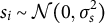 is the person random effect;
$d_{ij} \sim \mathcal {N}(0, \sigma _d^2)$
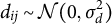 is the day random effect;
$\nu _{ij}$
 is the day-level AR(1) process with stationary variance
$\tau _d^2$
 and autoregressive parameter
$\phi _d$
 ,
$\omega _{ijk}$
 is the moment-level AR(1) process with stationary variance
$\tau _m^2$
 and autoregressive parameter
$\phi _m$
 ; and
${\varepsilon }_{ijk} \sim \mathcal {N}(0, \sigma _{\varepsilon }^2)$
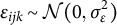 is the measurement error. All aforementioned random variables are assumed to be independent of each other and have finite variances.
Before deriving the correlation coefficients, some fundamental statistical concepts must be clarified.
A.1 Marginal versus conditional variance
To generalize the reliability results to the broader population of persons, days, and moments, we must consider the random mechanism that generates the observed scores. Formally, we can conceptually treat the observed score
$y_{IJK}$
 as a random variable, where I, J, and K are random indices representing a randomly drawn person, day, and moment, respectively. This means that
$y_{ijk}$
 is then a realization of
$y_{IJK}$
 when
$I=i$
 ,
$J=j$
 , and
$K=k$
 . We assume the probability of drawing any specific person from the population is uniform, as is the probability of drawing any specific day or moment. Under this fully marginal perspective, the variance of the person effect
$s_I$
 across the population is
$\operatorname {\mathrm {Var}}(s_I) = \sigma _s^2$
 .
Conversely, when we evaluate reliability strictly at the within-person level—meaning we consider the scores for a specific person i rather than the whole population—we condition on that specific person i. Under this condition, the variance of the person effect yields zero (i.e.,
$\operatorname {\mathrm {Var}}(s_I \mid I = i) = 0$
 ) because the person is fixed. However, the conditional variances of the other components (
$d_{IJ}$
 ,
$\nu _{IJ}$
 ,
$\omega _{IJK}$
 , and
${\varepsilon }_{IJK}$
 conditional on
$I=i$
 ) are not zero, because the days and/or moments have not been specified and thus remain random.
Note that for the simplicity of notation, in the main text and hereafter, we still use
$s_i$
 to denote the person effect for a random person i from the population
$\mathcal {S}$
 and the same for
$y_{ijk}$
 and the remaining random effects (i.e., d,
$\nu $
 ,
$\omega $
 , and
${\varepsilon }$
 ). If we want to denote a specific person i, then we condition on that person i in the variance or covariance,
$\operatorname {\mathrm {Var}}(\cdot \mid i)$
 or
$\operatorname {\mathrm {Cov}}(\cdot , \cdot \mid i)$
 , respectively.
A.2 Stationarity of the AR(1) process
An AR(1) process is stationary if its marginal distribution remains constant over time (specifically, it is weak stationary if its mean and variance are time-invariant). Taking the day-level AR(1) process
$\nu _{ij}$
 as an example, it is formulated as

where
$\tau _d^{\ast 2}$
 is the variance of the innovation (i.e., white noise) process
$\eta _{ij}$
 . By the definition of stationarity, the variance should be constant over time, meaning
$\operatorname {\mathrm {Var}}(\nu _{ij}) = \operatorname {\mathrm {Var}}(\nu _{ij'})$
 for all
$j, j' \in \mathcal {D}$
 . Therefore, we have

for all
$|\phi _d| < 1$
 . In the main text, we bypass the innovation variance
$\tau _d^{\ast 2}$
 and simply directly parameterize this constant marginal variance as
$\tau _d^2$
 .
Consequently, the covariance between two observations with a time lag of
$\Delta _{jj'} = |j - j'|$
 is given by

which is a geometric decay based on the autoregressive parameter
$\phi _d$
 . Note that if
$\Delta _{jj'} = 0$
 (i.e., on the same day), the covariance is exactly equal to the marginal stationary variance
$\tau _d^2$
 . By combining all days into a vector
$\boldsymbol {\nu }_i = (\nu _{i1}, \dots , \nu _{iD})^\top $
 , the constructed covariance matrix of the day-level AR(1) process perfectly corresponds to
$\boldsymbol {H}_d$
 presented in Section 3.1.
The identical stationarity principle applies to the variance and covariance of the moment-level AR(1) process,
$\omega _{ijk}$
 , when the autoregressive parameter
$|\phi _m| < 1$
 . Specifically,
$\operatorname {\mathrm {Var}}(\omega _{ijk}) = \tau _m^2$
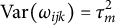 , and
$\operatorname {\mathrm {Cov}}(\omega _{ijk}, \omega _{ij'k'}) = \tau _m^2 \phi _m^{\Delta _{kk'}}$
 if measured on the same day (
$j=j'$
 ), and
$0$
 if measured on different days (
$j \neq j'$
 ). Correspondingly, combining all moments as a vector
$\boldsymbol {\omega }_{ij} = (\omega _{ij1}, \dots , \omega _{ijK})^\top $
 yields the covariance matrix
$\boldsymbol {H}_m$
 presented in Section 3.1.
A.3 The derivation of between-person reliability
Between-person test–retest reliability for single-item measures is conceptualized as the (marginal) correlation between two measurements for the same person taken at different time points (lagged by
$\Delta _{jj'}$
 days and
$\Delta _{kk'}$
 moments) across the population, which can be expressed as follows:

Note that the person i here is randomly selected from the people population
$\mathcal {S}$
 , not fixed.
The numerator in Equation (A.2) depends on whether the two moments occur on the same day or not. Following the principles outlined in Appendices A.1 and A.2, distributing the covariance yields:

where
$\delta _{jj'}$
 is the Kronecker delta, which equals 1 if
$j = j'$
 and 0 otherwise. The above equation shows that if the measurements are taken on the same day (
$j = j'$
 ), the covariance includes the person variance
$\sigma _s^2$
 , the day variance
$\sigma _d^2$
 , the day-level AR(1) variance
$\tau _d^2$
 (i.e.,
$\Delta _{jj'}=0, \phi _d^0=1$
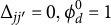 ), and the decayed moment-level AR(1) covariance
$\tau _m^2\phi _m^{\Delta _{kk'}}$
 . If the measurements are taken on different days (
$j \neq j'$
 ), the day effects
$d_{ij}$
 and
$d_{ij'}$
 are independent, and there is no covariance between moment processes because they occur on different days. Hence, the covariance merely includes the person variance
$\sigma _s^2$
 and the decayed day-level AR(1) covariance
$\tau _d^2\phi _d^{\Delta _{jj'}}$
 .
In contrast, based on the independence of the random components, the denominator in Equation (A.2) is the straightforward sum of all variance components:

Crucially, under the stationarity assumption, this variance is constant regardless of the specific time points (i.e.,
$\operatorname {\mathrm {Var}}(y_{ij'k'}) = \operatorname {\mathrm {Var}}(y_{ijk})$
 ).
Combining the numerator and denominator, we have the between-person reliability coefficient as follows:

Therefore, we get the general reliability coefficient under the correlation approach for the three-level LMM with two AR(1) processes. By setting
$\Delta _{jj'}$
 and
$\Delta _{kk'}$
 to specific values, we can get the specific reliability coefficients for different time intervals (e.g., instantaneity, moment-to-moment, day-to-day, and stability).
A.4 The derivation of within-person reliability
Within-person test–retest reliability for single-item measures can be defined as the correlation between two measurements for the same person taken at different time points (lagged by
$\Delta _{jj'}$
 days and
$\Delta _{kk'}$
 moments), conditioned on that specific person i, which can be expressed as follows:

The formulation mirrors the between-person reliability, except that the person i is fixed all along. It should be noted that because our current model assumes homogeneity of variances and autoregressive parameters across all individuals, the resulting within-person reliability coefficient is a single metric that technically applies to any person sampled from the population. However, this generalizability stems entirely from the model’s homogeneity constraints. If these assumptions were relaxed, for instance, by specifying person-specific innovation variances or person-specific AR parameters, the same derivation would naturally yield person-specific reliability coefficients.
The numerator in Equation (A.3) also depends on whether the two moments occur on the same day or not. Based on the principles in Appendices A.1 and A.2, distributing the conditional covariance yields:

Note that the person variance
$\sigma _s^2$
 is not included in the covariance because we have conditioned on a specific person i. Similarly, the denominator in Equation (A.3) is a conditional variance:

which is the sum of all variance components except the person variance
$\sigma _s^2$
 . Because of the stationarity assumption, this variance is also constant regardless of the specific time points (i.e.,
$\operatorname {\mathrm {Var}}(y_{ij'k'} \mid i) = \operatorname {\mathrm {Var}}(y_{ijk} \mid i)$
 ).
Combining the above results, the within-person reliability coefficient under the correlation approach for the three-level LMM with two AR(1) processes is given by

By setting
$\Delta _{jj'}$
 and
$\Delta _{kk'}$
 to specific values, we can get the specific reliability coefficients for different time intervals (e.g., instantaneity, moment-to-moment, and day-to-day, but not stability).
B Reliability estimation of negative affect in Exam Results Study
Estimates of reliability coefficients for the single-item negative affect assessment in the Exam Results Study

Table B1 Long description
The table is divided into two main sections: Single score and Daily average score.
Under Single score, the reliability coefficients include:
* rho sub 0 = R sub T M: Between-person mean 0.76 (0.05), H D I [0.69, 0.84]; Within-person mean 0.68 (0.06), H D I [0.60, 0.79].
* rho sub M (Delta sub k k’ = 1 to 9): Between-person means decrease from 0.63 to 0.50; Within-person means decrease from 0.52 to 0.35.
* R sub T D: Between-person mean 0.50 (0.03), H D I [0.45, 0.54]; Within-person mean 0.35 (0.04), H D I [0.30, 0.41].
* rho sub D (Delta sub j j’ = 1 to 8): Between-person means decrease from 0.38 to 0.23; Within-person means decrease from 0.19 to 0.01.
* rho sub infinity = R sub T P: Between-person mean 0.23 (0.05), H D I [0.14, 0.31]; Within-person data is not applicable.
Under Daily average score, the reliability coefficients include:
* rho sub overline D (Delta sub j j’ = 1 to 8): Between-person means decrease from 0.70 to 0.43; Within-person means decrease from 0.47 to 0.01.
All values include posterior standard deviations in parentheses and 95% posterior Highest Density Intervals in brackets.
Note:
$\rho $
 = reliability based on the correlation approach; R = reliability based on the variance partitioning approach; subscripts
$0$
 = instantaneity,
$\text {M}$
 = moment-to-moment;
$\text {D}$
 = day-to-day,
$\overline {\text {D}}$
 = day-to-day for average scores,
$\infty $
 = stability,
$\text {TM}$
 = momentary scores,
$\text {TD}$
 = daily score,
$\text {TP}$
 = personal trait scores;
$\Delta _{kk'}$
 = time lag between moments, and
$\Delta _{jj'}$
 = time lag between days.






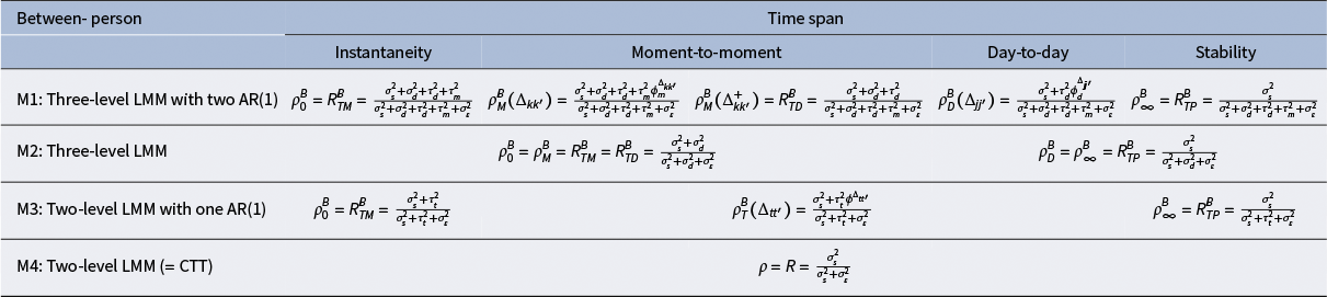
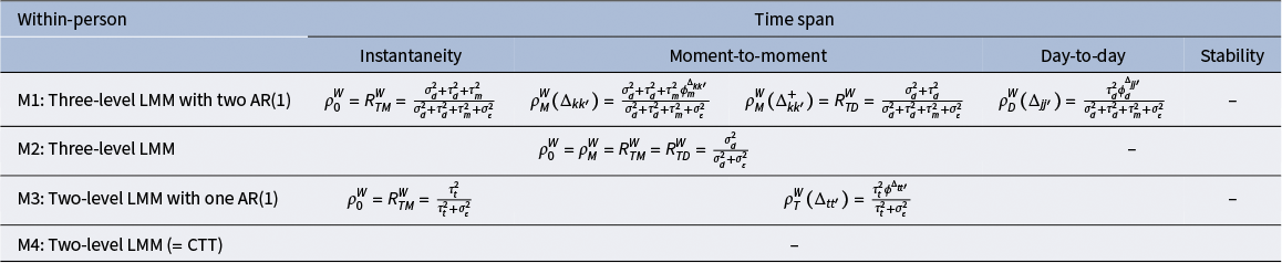
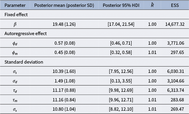
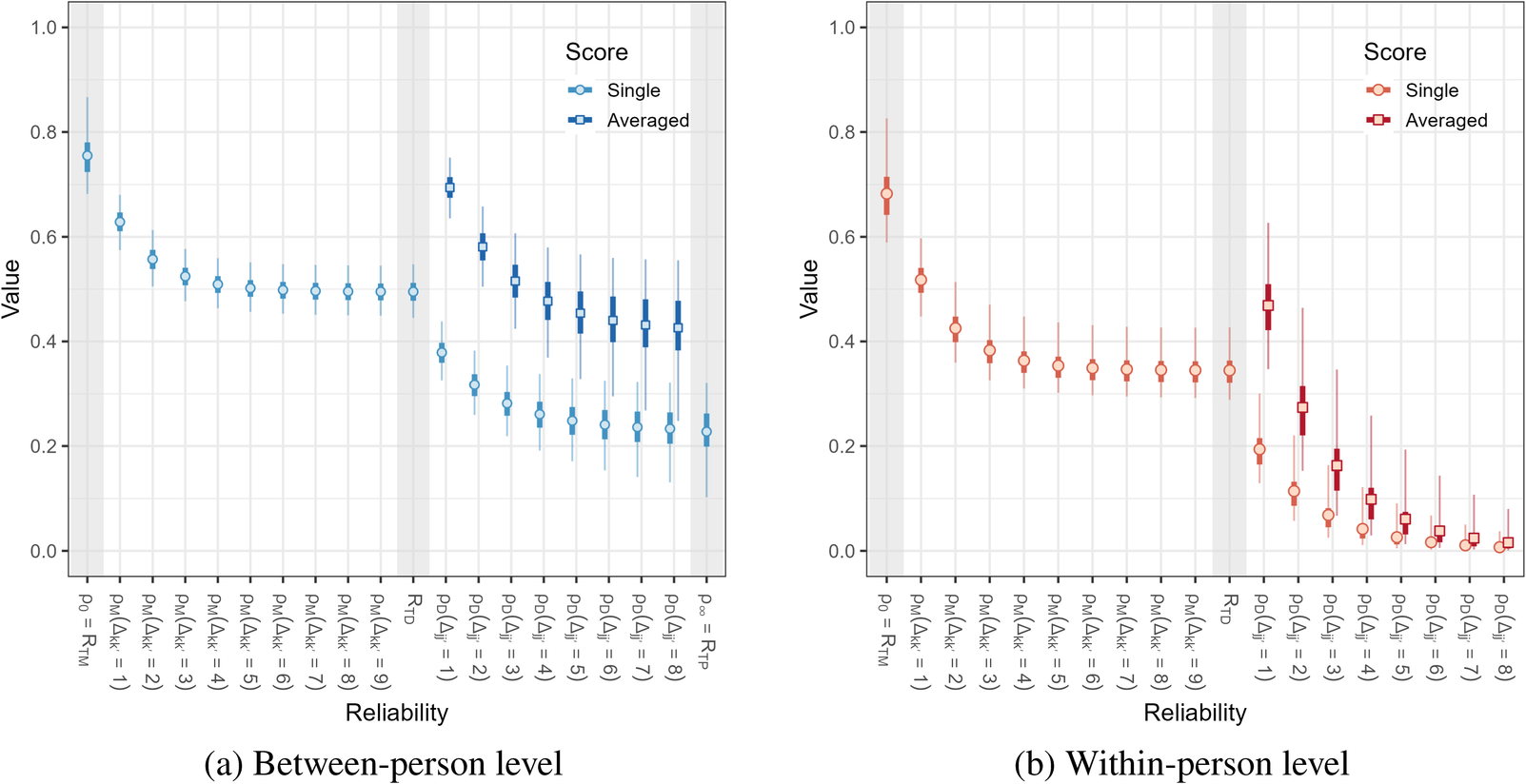


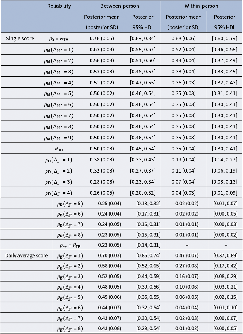

 Open access

