I. INTRODUCTION
Since its announcement three years ago, the materials genome initiative has resulted in a marked uptick in the number and quality of new materials discovered using theoretical approaches such as density functional theory (DFT) and calculated phase diagrams (CALPHAD). Recent reports have highlighted that, to fully realize the aspirations of mapping the materials genome, the theoretical–experimental loop must be closed.Reference Green, Hattrick-Simpers, Takeuchi, Barron, Joshi, Chiang, Davydov and Mehta1,2 In such closed-loop studies, experimental and theoretical work are carried out in parallel with curated data made available across the computation/experimentation divide to guide and refine the progress of both efforts.
High-throughput experimental (HTE) methodologies have been proposed by several recent reports as the key technology for providing the empirical databases and validation studies necessary to strengthen the computational aspirations of the MGI.Reference Green, Hattrick-Simpers, Takeuchi, Barron, Joshi, Chiang, Davydov and Mehta1–Reference Hattrick-Simpers, Wen and Lauterbach4 In the HTE approach, tens to hundreds of samples are synthesized in parallel, processed, and then rapidly characterized via either parallel or serial measurement techniques. The approach was initially bottlenecked by the lack of sufficiently reliable and rapid characterization tools, however today a myriad of such tools are readily available.Reference Green, Takeuchi and Hattrick-Simpers5–Reference Xiang, Sun, Briceno, Lou, Wang, Chang, Wallace-Freedman, Chen and Schultz8 HTE is now part of the standard industrial repertoire for novel material identification and process optimization with numerous examples of HTE leads being commercialized.Reference Arriola, Carnahan, Hustad, Kuhlman and Wenzel9,Reference Lauterbach, Sasmaz, Bedenbaugh, Kim and Hattrick-Simpers10
Rapid, automated characterization HTE techniques now permit 103 to 105 samples per day to be characterized for their figure of merit (FOM).Reference Kusne, Gao, Mehta, Ke, Nguyen, Nguyen, Ho, Antropov, Wang, Kramer, Long and Takeuchi11,Reference Shinde, Guevarra, Haber, Jin and Gregoire12 At this rate of acquisition, data analysis via traditional plotting software becomes prohibitively time consuming. In the case of relatively straight forward imaging measurements, simple algorithms can be used to collapse multidimensional datasets into a simplified FOM.Reference Holzwarth, Schmidt and Maier13,Reference Famodu, Hattrick-Simpers, Aronova, Chang, Murakami, Wuttig, Okazaki, Furuya, Knauss, Bendersky, Biancaniello and Takeuchi14 More complicated measurements, such as x-ray diffraction (XRD) and spectroscopic measurements, involve more complex methods of data analysis and remain an open challenge.
One major difficulty is phase identification as a function of composition and processing time/temperature. Currently, this critical step is mostly done by human experts who make judgments based on a variety of heuristics, such as peak location and peak shape. Many HTE studies focus on exploration of unknown material systems with potentially new phases/structures appearing.Reference Kan, Long, Steinmetz, Lofland and Takeuchi15 In such studies, various assisted and unassisted clustering analysis tools are used to expedite this analysis process by classifying different spectra based on their similarities, thus minimizing the total number of spectra that needed to be analyzed in detail.Reference Kusne, Gao, Mehta, Ke, Nguyen, Nguyen, Ho, Antropov, Wang, Kramer, Long and Takeuchi11,Reference Kan, Long, Steinmetz, Lofland and Takeuchi15–Reference Le Bras, Bernstein, Gomes, Selman and Van Dover18 Long et al. applied a non-negative matrix factorization (NMF) to the problem of analyzing x-ray microdiffraction (μXRD) patterns from a combinatorial materials library.Reference Long, Bunker, Li, Karen and Takeuchi19 NMF is a powerful technique for breaking diffraction or spectroscopic data down into a set of basis patterns but is known to not track peak shift. Examples of techniques that address peak shift include applied constraint programming and adaptable time warping (ATW). LeBras et al. applied constraint programming together with kernel methods and clustering to find K basis patterns that jointly compose N observed patterns while enforcing spatial and scaling constraints.Reference Le Bras, Damoulas, Gregoire, Sabharwal, Gomes and Van Dover20 This technique, similar to our approach, requires a smaller training set be specified and analyzed via machine learning techniques, as computational cost greatly increases as the sample set gets larger, in their study they applied a clustering approach to determine the training set. Baumes et al. proposed an ATW methodology for automatically deciphering XRD patterns from XRD data.Reference Baumes, Moliner and Corma21 Other unsupervised approaches include PCA, clustering, etc. as discussed by Barr et al.Reference Barr, Dong and Gilmore22 All these methods are unsupervised and depend on the available reference patterns or preclustering to identify base structures. Many of the previously reported clustering techniques rely on substantial postprocessing of the data (i.e., averaging, background subtraction, etc.) to provide accurate clustering results, inhibiting on the fly experimental design.
While clustering analysis has shown great potential for reducing the overall number of spectra analyzed, there are examples of HTE experiments (i.e., discovery of high-temperature oxidation-resistant alloys or the synthesis of a zeolite by statistical methods) where the desired structure is known and what is sought is a rapid method for identifying its existence in parameter space.Reference Metting, Bunn, Underwood, Smoak and Hattrick-Simpers23,Reference Corma, Diaz-Cabanas, Moliner and Martinez24 There are several examples in the literature of automated processes to expedite Rietveld refinement of powder diffraction patterns for phase identification, however, these techniques cannot be generalized to spectroscopic data.Reference Gilmore, Barr and Paisley25 To the best of our knowledge, until this moment an automated method for monitoring temporal phase transformation/formation in an HTE sample, combining the results from multiple structural measurements, has not been reported.
While there are many algorithms that can automatically perform postprocessing quickly, such as those available via MDI Jade for XRD data or GRAMS for spectroscopic data, the background subtraction from these algorithms needs to be reviewed and adjusted manually to ensure that no artifacts are created or important data are lost during this procedure. This can significantly lengthen the amount of time needed for postprocessing. In truly high-throughput experiments, turn over time between wafer measurements of less than an hour, accurately postprocessing the data in real-time could take longer than a measurement itself.
Instead of relying on either clustering or expert heuristic knowledge for phase identification, we developed a data-driven approach called AutoPhase for accurate, automated phase identification based on a supervised machine learning approach. In this process, the aforementioned phase identification problem is treated as a standard pattern classification problem. Initially, AutoPhase uses a raw training dataset that has been annotated by human experts for the presence and absence of phases. It then calculates thousands of features from the sample dataset describing a variety of factors that human experts use to identify different types of phases: such as the peak position, peak height, peak width, peak shapes, etc. After feature generation, we apply a feature selection algorithm called AdaBoost to automatically extract distinctive features. The selected features are then used to train a phase classifier model using AdaBoost for final phase identification.
Here we will describe a proof-of-principle study using AutoPhase to provide a comprehensive overview of the role of composition and heat treatment time on the high temperature oxidation of metal alloys in an HTE library investigated via multiple phase characterization techniques. Ni–Al binary thin-film composition-spread samples were monitored for oxidation at 1323 K using a combination of glancing incidence x-ray diffraction (GIXRD) and Raman/fluorescence spectroscopy to investigate the presence and time progression of oxide phases. The data were phase indexed by topical experts and fed into AutoPhase for verification. The phases observed by the two methods of analysis were then compared showing that AutoPhase, with sufficient input regarding what phases could be expected to form, showed better than 99% accuracy in identifying the presence of oxide phase in XRD studies. Raman/fluorescence data benefited from data postprocessing with accuracy better than 97%, however, even without postprocessing the accuracy was nearly 90%.
II. MODEL SYSTEM: COMPOSITION SPREAD OF Ni–Al AS OXIDATION-RESISTANT BOND COATS
The development of modern jet turbine engines represents one of the most challenging scientific endeavors of the 21st century. The operating temperature of turbines has increased from 1173 K in 1965 to 1773 K in modern engines owing to the need to maximize the thermodynamic efficiency of the engine.Reference Clarke, Oechsner and Padture26–Reference Goward29 The ultimate goal is to increase the engine operating temperature to 2273 K, which will require an entirely new class of materials for the turbines.Reference Perepezko30 Modern turbines are composed of a multilayer composite, which include a creep-resistant superalloy blade, a low thermal conductivity thermal barrier coating (TBC), and an adhesion layer, typically denoted as a bond coat. The bond coat is a metallic coating applied directly to the superalloy, which forms a thermally grown oxide (TGO) at its interface with the TBC under normal operating conditions. The TGO facilitates adhesion between the metallic superalloy and the ceramic TBC during temperature cycling, while also inhibiting oxidative degradation of the underlying superalloy.
The composition of the bond coat is chosen to closely match that of the superalloy, and a great deal of work has focused on the Ni–Al system since Ni-based superalloys are commonly used in current generation turbine engines.Reference Lehnert and Meinhardt31–Reference Gleeson, Mu and Hayashi33 The fundamental FOM for a TGO is its ability to rapidly nucleate a uniform, compact, and defect-free oxide.Reference Monceau, Oquab, Estournes, Boidot, Selezneff, Thebault and Cadoret34,Reference Zhang, Pint, Haynes and Wright35 The actual oxidation process that occurs is quite complex with the diffusion of metals throughout the bond coat, the precipitation of secondary metallic phases, formation of nonprotective oxides, the formation of oxides which are the precursors to the protective oxide, and the protective oxides themselves. The process is dynamic in nature and extremely sensitive to composition. An alloy that forms protective α-Al2O3 may become Al deficient and begin to form nonprotective oxides after a period of time. Additionally, subatomic variations in the Al content and subtle changes to alloy processing can dramatically alter the phase of the TGO.Reference Jiang, Sordelet and Gleeson36–Reference Dryepondt, Rouaix-Vande Put and Pint41 The complexity of the phase space that is required to be explored in this system makes it an ideal candidate for the use of HTE methodologies.
We have recently demonstrated a proof-of-principle study using a combination of diffraction and spectroscopic approaches to elucidate oxide formation on high-temperature Ni–Al alloys as a function of composition and oxidation time.Reference Metting, Bunn, Underwood, Smoak and Hattrick-Simpers23 The study is an excellent example for the need and application of machine learning algorithms to large datasets, as it involves the systematic discrimination of 7 potential metallic phases and 7 oxide phases from one another. Information about the metallic/oxide phase is extracted from 3 distinct datasets, with no single dataset containing all of the necessary information. Additionally, each set exhibits substantial peak overlap as a function of time as well as peak shift, a particular challenge for current clustering techniques. This problem becomes exacerbated when one moves into ternary composition spreads or the recently identified multernary, high-entropy alloy systems.Reference Hattrick-Simpers, Jun, Murakami, Orozco, Knauss, Booth, Greve, Lofland, Wuttig and Takeuchi42,Reference Yeh, Chen, Lin, Gan, Chin, Shun, Tsau and Chang43
III. EXPERIMENTAL
A. NiAl bond coats
Polycrystalline Inconel alloy 600 “tokens” were cut from an Inconel sheet using a drill press and mechanically polished down to a 1 μm grit. The samples were then mounted to a glass slide and placed inside a 5-gun UHV sputtering chamber, base pressure of 1.87 × 10⁻⁶ Pa, in the sputter-up geometry. To promote adhesion of the Ni and Al to the Inconel substrate, the chamber was heated to 773 K before deposition. The tokens and the glass slide were then deposited on by simultaneously RF sputtering Ni at 190 W and DC sputtering Al at 100 W under a pressure of 0.667 Pa for 121 min producing a film with an average thickness of 1 μm.
XRD and energy dispersive spectroscopy (EDS) were performed on the glass slide to determine the samples' phase and composition without interference from the Inconel substrate. The tokens were heat treated 4 times in a quartz tube furnace under atmosphere at 1323 K for cumulative times of 5, 10, 20, and 30 min. The tokens were air quenched and characterized using Raman spectroscopy, fluorescence, and GIXRD between time steps. Raman and fluorescence data were taken with the same micro-Raman system using a 441.6 nm blue laser and a 632.8 nm red laser, respectively. The data from the 632.8 nm laser measurements are referred to here as the fluorescence data due to the excitation of fluorescence from Al2O3 species.
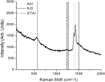
A detailed description of the experimental procedure can be found in Ref. Reference Metting, Bunn, Underwood, Smoak and Hattrick-Simpers23. To show how the data were analyzed, a typical fluorescence spectrum from an oxidized NiAl bond coat is given in Fig. 1 along with the reference peak locations of the oxide species. In this plot, the main peaks for NiO and α-Al2O3 are easily identified with minimal overlaps. However, the peak located at 1500 cm−1 can be attributed to both the NiO magnon and γ,θ-Al2O3 fluorescence. In such cases, the expert had to use a heuristic that referenced other peaks in the spectrum.
A plot of the 52 at.% Ni 10 min annealed fluorescence spectrum. The vertical lines represent the position of reference peaks used to identify the presence of different species, where AAl: α-Al2O3, NiO: nickel oxide, and GTAl: γ,θ-Al2O3. The peak located at 1500 cm−1 can be indexed to both nickel oxide and γ,θ-Al2O3.

B. AutoPhase
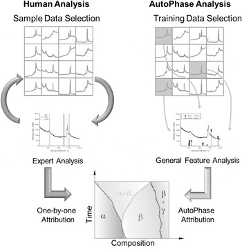
In our phase identification approach, the goal is to generate a phase identification/classification function from a given feature set and a training set of positive/negative samples that do/do not contain a specific phase. To succeed in this goal, the AutoPhase algorithm uses several steps including data preprocessing, feature extraction, AdaBoost-based feature selection, and classifier training (Fig. 2).
A flow diagram of the general steps used in AutoPhase vs. human analysis.

For preprocessing, a moving average noise reduction filter was applied to the training and prediction datasets to minimize the possibility of evaluating noise as an important feature. The number of data points that the moving average filter used, referred to here as the smoothing window data points, was entered into AutoPhase and could be adjusted based on the average noise of the datasets.
Similar to human experts, the phase identification capability of AutoPhase depends on a set of features extracted from the sample. The existence of peaks and the slopes (down, up, or flat) was used to describe the Raman, fluorescence, and XRD data. AutoPhase used the training datasets to identify these important features for a given, identified species using a “sliding” trend window and a trend threshold. The “sliding” trend window is the number of data points around a central data point for which the trends will be evaluated, similar to the smoothing window data points. The trend threshold represents a change in an intensity value synonymous with the variations of the noise in the data. Every sliding window is analyzed for the existence of these features. For peak features, the following equation was used:
 $$F_{{\rm{peak}}} \left( {x_{\rm{c}} } \right) = \left\{ {\matrix{ {I\left( {x_{\rm{c}} } \right);\quad I\left( {x_{\rm{c}} } \right) - I\left( {x_{\rm{c}} + \Delta x} \right) > T{\rm{and}}I\left( {x_{\rm{c}} } \right) - I\left( {x_{\rm{c}} - \Delta x} \right) > T} \cr {0;\quad \quad \quad \quad \quad \quad \quad \quad \quad \quad \quad \quad \quad \quad \quad \quad \quad \quad \quad {\rm{otherwise}}} \cr } } \right.\quad {\rm{,}}$$
where x c is the central x-value of the sliding window, F peak is a peak feature value, I is an intensity value at a point, Δx is the x-range absolute difference from the central x-value to the min/max x-value of the sliding window, and T is the trend threshold. To determine the value of slope features of a trend window, all the slope trends in the data were determined. Identification of a slope trend at any point, j, in the data was determined by:
 $$S\left( {x_j } \right) = \left\{ {\matrix{ {{\rm{down}};\quad I\left( {x_{j + 1} } \right) - I\left( {x_{j - 1} } \right) \lt - T} \cr {{\rm{flat}};\quad - T \le I\left( {x_{j + 1} } \right) - I\left( {x_{j - 1} } \right) \le T} \cr {{\rm{up}};\quad I\left( {x_{j + 1} } \right) - I\left( {x_{j - 1} } \right) > T} \cr } } \right.\quad {\rm{,}}$$
where S is the recorded slope trend. For a trend window, the sum of all like slope trends in a sliding window was recorded so that there were values for the down, flat, and up trends. The values for the number of data points in the smoothing and sliding windows and the trend threshold for each type of data are given in Table I.
The smoothing and trend window and trend threshold values for each type of data that AutoPhase was used to analyze. For the smoothing and trend window, the left column represents the number of data points including the central point and the right column represent the equivalent x-range that is covered. The values for these parameters change for each specific data type based on the noise and how defined and clustered the expected peaks for each data type was.

After all possible features have been determined, AutoPhase selects the most distinguishing features for building the final phase classifier via supervised learning. In the current implementation, AutoPhase uses AdaBoost for feature selection and classifier training. AdaBoost is an ensemble learning algorithm that combines multiple weak classifiers into a strong classifier.Reference Freund and Robert44 It does so by adaptively adjusting the contribution of the weak classifiers iteratively and comparing the resulting phase/species predictions with the labeled training datasets. The weights of the training samples, which are misclassified by the current weak learner, were increased while the weights of the correctly classified samples were decreased. This forces succeeding weak classifiers to focus on the hard examples in the training set. This process is repeated until AutoPhase correctly identifies all of the species in the training sets. We used single feature classifiers as the base classifier and train the ensemble classifier using the AdaBoost procedure. A more detailed explanation of how the contributions of the weak classifiers are adjusted, how the ensemble classifier is adjusted, and the pseudocode for the AdaBoost algorithm is given in the supplemental material. AdaBoost requires no prior knowledge about the weak learner and can be easily combined with other methods for classification, such as support vector machines. The reason for using AdaBoost for supervised feature selection is its ability to be generalized.
IV. RESULTS AND DISCUSSION
A. Feature determination
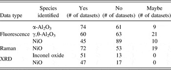
For validation purposes, an expert analyzed all of the data to identify the presence of each species. The results of this analysis are given in Ref. Reference Metting, Bunn, Underwood, Smoak and Hattrick-Simpers23, but in summary, the expert identified the presence or absence of NiO, α-Al2O3, and γ,θ-Al2O3 peaks in the fluorescence data, NiO in the Raman data, and NiO and the substrate-Inconel oxide in the XRD data. The expert labeled each dataset with a Yes, No, or Maybe for the presence of each species (Table II). The datasets labeled “Maybe” were not included in training datasets or considered in the accuracy of AutoPhase.
The quantities in the table show the number of datasets that the human expert labeled with a “Yes”, “No”, or “Maybe” for the presence of each species in a data type. The datasets labeled with a maybe were not included in the training or prediction datasets for AutoPhase.

For a given data type, the datasets were randomly split into three equal sized subsets initially. This process was repeated for the number of species identified in a given data type and for every data type, resulting in 1 set of subsets for the Raman data, 3 sets of subsets for the fluorescence data, and 2 sets of subsets for the XRD data. Two of the subsets of each set were then chosen as the training dataset, and the remaining set was chosen as the prediction set. The learning and prediction sets were used by AutoPhase to perform species/phase identification. AutoPhase performed phase identification on 3 separate training datasets (the paired combination of the three subsets) and corresponding prediction sets for each identified species and data type. It should be noted that an analysis of the effectiveness of the AutoPhase algorithm as a function of the training data size was performed, and is reported in the supplementary material.
After the features and the corresponding contributions in the training datasets were determined using the methodology described above, AutoPhase was used to evaluate the existence of each identified species for the prediction datasets. Ideally, AutoPhase will predict accurately on unprocessed datasets, since background subtractions of the Raman and fluorescence data are time consuming, particularly when hundreds or thousands of data with distinct background signatures are considered. Therefore, the as-taken data were initially analyzed by AutoPhase to determine its predictive capability in the presence of nonlinear backgrounds. To improve performance, AutoPhase was subsequently used to analyze datasets that had undergone a multistep data processing procedure, which consisted of a background subtraction, shot noise reduction, and data truncation. Please note that, to preserve the regular partitioning of the data, all of the fluorescence data are displayed here in Raman shift instead of absolute wave length as fluorescence phenomena are commonly reported.
B. Feature analysis
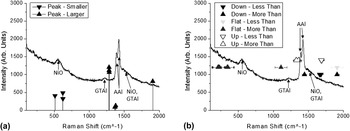
The key to the phase/species identification for AutoPhase is the determination of features that it deems important (have a high contribution). While materials engineers tend to use reference peak data, such as XRD data from the Inorganic Crystal Structure Database, or theoretically predicted structures, AutoPhase does not.Reference Jain, Ong, Hautier, Chen, Richards, Dacek, Cholia, Gunter, Skinner, Ceder and Persson45,46 Instead, it determines the features that indicate the presence of a species based on contrasts in the training data, identifying up to 100 highly contributing features. Therefore, it is important to review and analyze the contributing features that AutoPhase has chosen and validate that these features make physical sense. Due to the large number of datasets and the corresponding important features (3 sets per species, 18 total sets, up to 100 important features/set), only a full analysis of the 50 most contributing features of the α-Al2O3 unprocessed fluorescence data will be presented here (Fig. 3), as they exhibit the poorest performance of the three data types. A summary of the feature analysis of the other species is given in the supplementary material.
The 50 most contributing features that AutoPhase identified for a subset of the α-Al2O3 fluorescence data. For illustration purposes, the 52 at.% Ni 10 min annealed fluorescence spectra are plotted along with the features. (a) The peak features that AutoPhase identified as highly contributing and the relative value a peak needs to lie above (pointing up triangle) or below (pointing down triangles) to contribute to the existence of α-Al2O3. (b) The slope features that AutoPhase identified as highly contributing, the intensity values of these datasets were arbitrary, but denote whether AutoPhase identified an downward (intensity of 1200), flat (intensity of 1400), or upward (intensity of 1600). The bars to the left and right of the data point represent the threshold x-range in the trend window (± 45 cm−1 around the central point) that the data need to be more or less than to contribute to the existence of α-Al2O3. The text labels represent the identity of the peaks, where NiO: nickel oxide; GTAl: γ,θ-Al2O3; and AAl: α-Al2O3.

For illustration purposes, the 52 at.% Ni 10 min annealed fluorescence spectra, as well as the peak identities, are plotted along with the features in Fig. 3. The peak features that AutoPhase identified as highly contributing are shown in Fig. 3(a). The intensity value of the peak feature data points represents the threshold intensity value for a peak. This threshold value determines whether the data should contribute to or take away from the identification of α-Al2O3 in the dataset by deciding if the peak intensity should be above (pointing up triangles) or below (pointing down triangles) an intensity value. In contrast to the metric used by traditional materials scientists, AutoPhase is more likely to identify the presence of α-Al2O3 if the NiO peak at 566 cm−1 Raman shift is suppressed and if there are very strong γ,θ-Al2O3 peaks at 1220, 1250, and 1265 cm−1 Raman shift. AutoPhase also uses the traditional metric to identify the presence of α-Al2O3 by searching for the 1389 cm−1 peak: a reference α-Al2O3 peak.
Although it is unexpected that the suppression of NiO and presence of γ,θ-Al2O3 would be chosen as discriminating features for α-Al2O3, there is a physical rationale for this to be the case. The suppression of the NiO peak would be expected in the presence of α-Al2O3 since the latter is considered a passivating oxide. On the other hand, the γ,θ-Al2O3 phases are well known to be precursors for the high temperature formation of α-Al2O3 and thus their presence is correlated to α-Al2O3. Therefore, the peak criterion selected by AutoPhase is reasonable and highly physical. The peak feature located at 1906 cm−1 Raman shift is an exception to this conclusion, as it lacks an obvious interpretation. We attribute this feature to the variations in background that AutoPhase erroneously identifies as correlated to the presence of a species.
The slope features that AutoPhase identified as highly contributing are shown in Fig. 3(b). The y-intensity values of these slope features on the figure are arbitrary but denote whether AutoPhase identified a downward (intensity of 1200), flat (intensity of 1400), or upward (intensity of 1600) slope. The bars to the left and right of the data point represent the threshold x-range in the trend window (± 45 cm−1) around the central point. The evaluation that a species is present increases if the number of correlating trend features (down, flat, up) in the trend window is greater/less than the trend threshold of the “More Than”/“Less Than” logically modified slope features. The number of correlating trend features in the trend window is determined by the calculation of S.
Similar to the peak features, the slope features show that AutoPhase is more likely to identify the presence of α-Al2O3 if there is suppressed oxide growth. However, the unique peak shape of the reference α-Al2O3 peak is considered more descriptive of α-Al2O3. The upward slope features located at 1326 and 1360 cm−1 are located at the beginning of the α-Al2O3 peaks, and the downward slope features located at 1659 and 1678 cm−1 are between the two reference fluorescence peaks located at 1265 and 1500 cm−1. These two slope features both are direct signs of the presence of the α-Al2O3 reference peak.
Unlike the peak feature, most of the slope features are outside the range of the peak data and thus are related more to the background of the data. These slope features are nonphysical and are more susceptible to the large, nonlinear changes in the background than the peak features. Although some of the important features identified by AutoPeak may be due to background changes in the data, the determination of multiple important features for phase identification can correct for effects of the nonphysical features, as evidenced by the high overall prediction rate.
The overall analysis of the most contributing features for the α-Al2O3 fluorescence data shows that AutoPhase identifies physically reasonable and sensible features to make phase/species predictions. Furthermore, it also shows that effects from the background in unprocessed samples can lead AutoPhase to identify highly contributing features that lack obvious physical interpretation. Similar results were found for the Raman and XRD data, although the latter sets of data tend to exhibit less complicated backgrounds.
C. AutoPhase performance
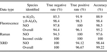
AutoPhase was used to evaluate the identity of all species present in the datasets. To evaluate the performance of AutoPhase, the true negative rate, the true positive rate, and the accuracy were calculated for each individual species as well as for the overall types of dataset (Raman, fluorescence, and XRD), and are shown in Table III. A more detailed table, with the number of datasets predicted correctly, is given in the supplementary material.
The true negative rate, true positive rate, and accuracy for all the identified species and data types of the predictions from AutoPhase for unprocessed data.

The true negative/positive rates are the percentages of the data labeled without/with the existence of a phase and predicted correctly by AutoPhase. They are calculated by:
 $${R_{{\rm{TN}}}} = {{{A_{\rm{N}}}} \over {{T_{\rm{N}}}}}\quad {\rm{,}}$$
 $${R_{{\rm{TP}}}} = {{{A_{\rm{P}}}} \over {{T_{\rm{P}}}}}\quad {\rm{,}}$$
where R TN and R TP are the true negative/positive rates for a given dataset type and species, respectively; A N and A P are the number of datasets that AutoPhase identified without/with the existence of a given species, respectively; and T N and T P are the total number of datasets that the expert identified without/with the given species for a given dataset type and species. For an overall type of data, A N and A P were the number of datasets that AutoPhase correctly predicted, and T N and T P were the total number of datasets labeled for that species.
The accuracy is the percentage of the data that AutoPhase correctly labeled and is calculated by:
 $${R_{{\rm{Pr}}}} = {{{A_{{\rm{Pr}}}}} \over {{T_{{\rm{Pr}}}}}}\quad {\rm{,}}$$
where R Pr is the accuracy for a given dataset type and species, A Pr is the total number of datasets that AutoPhase identified correctly for a given species, and T Pr is the total number of datasets that the expert identified. For an overall type of data, A Pr was the total number of datasets in a specific data type (Raman, fluorescence, XRD) in which AutoPhase correctly predicted all species, and T Pr was the total number of datasets that the expert identified for the existence of all species.
Table III shows that AutoPhase had the lowest prediction rate for the fluorescence data, and had a high prediction rate for the XRD and Raman data. Overall, AutoPhase had the lowest prediction rate for the α-Al2O3 fluorescence data, with an accuracy of 88.9%.
The relative performance of AutoPhase for the three different data types is unexpected. AutoPhase performed best for the XRD data, which is the hardest dataset to analyze by human eye due to the quantity of peaks and the potential for overlap. Conversely, AutoPhase had the lowest prediction rate for α-Al2O3 in the fluorescence data, which is the easiest of the species to identify in the fluorescence data by human eyes due to the sharp, double peaks that indicate α-Al2O3 existence. AutoPhase analyzes XRD data very well because it looks for the contrast between different datasets to identify the highly contributing features, meaning it disregards overlapped peaks and focuses automatically on nonoverlapped peaks. Peak sharpness and low background also contributed to AutoPhase's performance in comparison to the broad peaks and unpredictable background found in the Raman and fluorescence data.
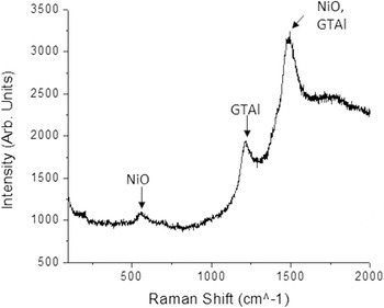
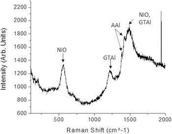
To evaluate why AutoPhase performed relatively poorly for the identification of α-Al2O3 in the fluorescence datasets, the misidentified samples were plotted and analyzed for common features. A representative plot of the trend in the fluorescence data that returned a false positive error is shown in Fig. 4. Here, the suppression of NiO and presence of γ,θ-Al2O3 are taken by AutoPhase as indications of α-Al2O3 growth despite no peaks for the phase being present. A representative plot of the trend in the fluorescence data that returned a false negative error is shown in Fig. 5. Here, an unusually high intensity NiO peak, a large γ,θ-Al2O3 peak, high background, and poorly defined α-Al2O3 peaks resulted in α-Al2O3 not being identified. Normally, the presence of a large NiO peak is a good indication that a protective α-Al2O3 has not formed despite the presence of its peaks in the spectrum. Interestingly, false negative and false positive errors occurred in the datasets that had good initial γ,θ-Al2O3 growth, but upon further annealing transitioned to majority NiO growth, possibly due to spallation or Al depletion at the surface of the metal.
A plot of the 63 at.% Ni, 5 min annealed data, which shows the general trends in the fluorescence data that lead to a false positive error in AutoPhase. The general trend of the data that lead to the false positive in AutoPhase is described by the suppression of the NiO peak at 566 cm−1 Raman shift and the γ,θ-Al2O3 fluorescence peaks at 1220 and 1500 cm−1 Raman shift. The text labels represent the identity of the peaks, where NiO: nickel oxide and GTAl: γ,θ-Al2O3.

The general trend in the fluorescence data that lead to a false negative error in AutoPhase. The plot is of a 42 at.%, 10 min annealed data. The trends in the data that lead to the false negative are the existence of a strong NiO peak at 566 cm−1 Raman shift and the slight α-Al2O3 peaks at 1389 and 1426 cm−1 Raman shift. The text labels represent the identity of the peaks, where NiO: nickel oxide; GTAl: γ,θ-Al2O3; and AAl: α-Al2O3.

For all of the other species, no discernible trend in the ill-identified species could be made, and misidentification was attributed to a combination of background effects and unoptimized AutoPhase input parameters (shown in Table I). These misidentified datasets are shown in the supplementary material. Despite the relatively high rate of misidentification of α-Al2O3, the prediction rate for all other species was above 97%. Based on the above analysis, the primary source of error for AutoPhase was the presence of shot noise in the spectrum and the irregular background of the fluorescence data.
D. Data processing and predictions
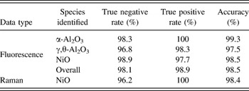
Both the Raman and fluorescence data went through a data processing procedure to investigate the potential for improving the accuracy of AutoPhase by eliminating the background and shot noise. No data processing was performed on the XRD data, as it was well predicted without data processing. The data were first truncated so that only points with a Raman shift between 450 cm−1 and 1650 cm−1 were evaluated. This region was chosen to encompass all of the major peaks and to exclude the effects of the notch filter at low wave numbers. Next, shot noise was manually eliminated and an 8 set, multisectional, linear background subtraction was performed. Additionally, one spectrograph was thrown out, due to instrumental error during acquisition. The processed data were then split into training and predictive sets as described above. It should be noted that no changes were made to the input values for AutoPhase. The true negative rate, true positive rate, and accuracy were then calculated and are tabulated in Table IV.
The true negative rate, true positive rate, and accuracy for all the identified species of the processed fluorescence and Raman and XRD data types of the predictions from AutoPhase. There is no field for the XRD data, as no further data processing was performed on the XRD data.

Table IV shows that the accuracy for α-Al2O3 increased by 10.4% while γ,θ-Al2O3 and NiO were predicted at roughly the same rate for the postprocessed fluorescence. The overall effect is that the accuracy for all fluorescence data increased by 3.3%. The increase in the accuracy of the α-Al2O3 fluorescence data shows that, by removing shot noise and the nonlinear background, Autophase predicts nearly identically to a topical expert. No systematic trends in the erroneously labeled datasets were identified, and are largely attributed to excessive noise and the need to further optimize AutoPhase input parameters.
This indicates that performing time intensive data processing maximizes the accuracy of AutoPhase predictions in some cases, such as on the α-Al2O3 fluorescence data. Postprocessing, a minimum prediction rate of 97.5% for all of the species and the lowest overall prediction rate of 98.4% were observed. However, for the identification of trends in large datasets, AutoPhase performs adequately on unprocessed data and can provide an overview of temporal performance across multiple datasets.
E. Future works
In the current work, AutoPhase was used to analyze 144 Raman datasets, 144 fluorescence datasets, and 64 XRD datasets. AutoPhase requires 40–200 training sets to be able to ensure that the important features are identified, which means in the current work the training sets were large compared to the predictive sets. In the future, AutoPhase will be applied to monitor the formation of oxides and phase metallic phase transformations observed using in situ synchrotron diffraction datasets (>1200 datasets). Here, depending upon the complexity of the alloy, less than 200 datasets will be used as training.
A central limitation to AutoPhase is that the training dataset has to be representative of the significant changes in the data and contain all identifiable species present in the data. If the data in the training set do not contain a significant change, then AutoPhase will have no way to “learn” how to relate this change to the identity of a species. If a “new” phase is encountered outside of the training set, then AutoPhase will not try to analyze and identify this species in the prediction dataset. This problem can be overcome by initially screening the data via hierarchal clustering or automated peak fitting algorithms to determine a training set that sufficiently spans the overall dataset. Such approaches have been applied previously with great success in the field.Reference Long, Bunker, Li, Karen and Takeuchi19 AutoPhase would then be able to step through all possible datasets and provide a full delineation of the phases present. In the context of on-the-fly experimental design, where new datasets are being generated in parallel with data analysis, the peak characteristics in each new dataset could be compared to those present in the original training set. The presence of new peaks would trigger an additional training run.
V. CONCLUSIONS
A novel machine learning algorithm, AutoPhase, has been constructed and used to identify the presence of different phases/species in Raman, fluorescence, and XRD data taken during a NiAl bond coat oxidation study. AutoPhase made phase/species identifications by creating a set of important features learned from a training dataset. These features included peak type and slope type features. The most important features that AutoPhase identified were evaluated to ensure that they were physically reasonable and could be reasonably used to identify the phase/species for each dataset. It was found that, on the whole, AutoPhase did identify physically reasonable important features. It was also found that in the Raman and fluorescence data the presence of shot noise and a highly varying background led AutoPhase to identify some important features that were erroneous. In-depth analysis of the accuracy of the algorithm was evaluated by comparing the identification of species in the datasets by a human versus the AutoPhase identified species. It was found that for the raw fluorescence data AutoPhase had an accuracy of 88.9% for α-Al2O3; 98.4% for γ,θ-Al2O3; and 98.5% for NiO. For the raw Raman data, the NiO was predicted with a 97.6% accuracy. For the XRD data, it was found that AutoPhase had an accuracy of 100% for the Inconel oxide and 98.4% for NiO. The low prediction rate for the α-Al2O3 fluorescence data was found to be due to an over-emphasis on the nonexistence of NiO; the existence of γ,θ-Al2O3; and shot noise in the raw data. To improve the overall performance of AutoPhase, the Raman and fluorescence data were background subtracted, truncated and had shot noise removed. After data processing, the accuracy of each species was evaluated again. It was found that the fluorescence accuracy for α-Al2O3 increased by 10.4% and remained roughly the same for NiO and γ,θ-Al2O3. This increased the overall performance of the algorithm so that it had an overall accuracy of 98.5% for the fluorescence data and an accuracy of 98.4% for the Raman data. This increase in the overall performance of the accuracy validated that the performance of AutoPhase could be significantly increased if the data were properly processed. However, AutoPhase shows promise in the field of on-the-fly data analysis, as preprocessed accuracies were all in excess of 89%.
Supplementary Material
To view supplementary material for this article, please visit http://dx.doi.org/jmr.2015.801.
ACKNOWLEDGMENTS
Hattrick-Simpers would like to acknowledge the support by the US National Science Foundation under grant DMR 1439054 and the South Carolina SmartState™ center for Strategic Approaches to the Generation of Electricity (SAGE).