1. Introduction
Due to the lack of any complete theory, the asymptotic behaviour of the zero-pressure-gradient (ZPG) turbulent boundary layer (TBL) in the limit of infinite Reynolds number has received sustained attention over the last century. In this paper we will be concerned primarily with the asymptotic behaviour of quantities that appear in the Reynolds-averaged mean momentum equation and in particular with the streamwise normal Reynolds stress
 $\langle uu\rangle$
. Even on this restricted subject, a complete bibliography is beyond the scope of any research paper. Instead, we only give an incomplete list of people who have contributed to the description of high-Reynolds-number TBLs, among them Prandtl (Reference Prandtl1925), Millikan (Reference Millikan1938), Clauser (Reference Clauser1956), Coles (Reference Coles1956), Rotta (Reference Rotta1962) and Mellor (Reference Mellor1972), to name just a few who developed the classical two-layer description of the streamwise mean velocity
 $U$
, with an inner or wall layer and an outer ‘wake’ region, joined across an overlap layer in which
 $U$
is given by the well-known logarithmic law. Here and in the following
 $(U,V,W\equiv 0)$
and
 $(u,v,w)$
are the mean and fluctuating velocity components in the streamwise, wall-normal and spanwise directions
 $(x,y,z)$
. Alternative mean velocity laws have been proposed by Barenblatt (Reference Barenblatt1993), Barenblatt et al. (Reference Barenblatt, Chorin, Hald and Prostokishin1997), George & Castillo (Reference George and Castillo1997) and George (Reference George2006), among others (for a discussion of the different approaches, see, e.g., Monkewitz, Chauhan & Nagib Reference Monkewitz, Chauhan and Nagib2008), while alternatives to the classical two-layer structure have been considered by Klewicki et al. (Reference Klewicki, Fife, Wei and McMurtry2007) and Klewicki (Reference Klewicki2013), for instance. Since the focus of this paper is the streamwise Reynolds stress
 $\langle uu\rangle$
, the detailed asymptotics of the mean velocity is of secondary interest here, except in appendix B where the classical inner–outer layer description is used to obtain the large-Reynolds-number asymptotic expansions of the shape factor and of the streamwise derivative of the displacement thickness. The rationale for this choice is its consistency with modern singular perturbation theory (see, e.g., Kevorkian & Cole Reference Kevorkian and Cole1985), where the number of primary layers equals the number of independent wall-normal length scales.
The normal stress
 $\langle uu\rangle$
has most often been scaled with the friction velocity squared,
 $u_{{\it\tau}}^{2}\equiv {\it\tau}_{w}/{\it\rho}$
, where
 ${\it\tau}_{w}$
is the wall shear stress and
 ${\it\rho}$
the constant fluid density. Based on experimental data, other scalings have been proposed, e.g. with
 $U_{\infty }u_{{\it\tau}}$
by DeGraaff & Eaton (Reference DeGraaff and Eaton2000), and even outer scaling with
 $U_{\infty }^{2}$
has been discussed as it leads to the best collapse of experimental
 $\langle uu\rangle$
data in the outer part of the TBL (see, e.g., figure 7 of Monkewitz, Chauhan & Nagib Reference Monkewitz, Chauhan and Nagib2007). For the shape of
 $\langle uu\rangle$
in the outer part of the TBL, a universal logarithmic law has been derived from the so-called ‘attached eddy model’ (see, e.g., Bradshaw Reference Bradshaw1967; Perry, Henbest & Chong Reference Perry, Henbest and Chong1986; Marusic & Perry Reference Marusic and Perry1995; Nickels et al.
Reference Nickels, Marusic, Hafez, Hutchins and Chong2007; Marusic et al.
Reference Marusic, McKeon, Monkewitz, Nagib, Smits and Sreenivasan2010; Hultmark Reference Hultmark2012; Banerjee & Katul Reference Banerjee and Katul2013; Marusic et al.
Reference Marusic, Monty, Hultmark and Smits2013, and references therein).
Surprisingly, the determination of formal asymptotic expansions for the different quantities in the Reynolds-averaged momentum equation has received comparatively little attention. The pioneering developments were carried out by Mellor (Reference Mellor1972), who recognized that proper expansions had to proceed in powers of two small parameters, the inverse Reynolds number and the inverse logarithm of the Reynolds number. However, it has been difficult to verify Mellor’s asymptotic expansions beyond the leading terms due to a lack of reliable high-Reynolds-number data. With the steady increase of the Reynolds number of direct numerical simulations (DNS), the improvement of probes and of the correction schemes for systematic errors, new wind tunnel experiments and, most importantly, independent skin friction measurements, notably by the oil film technique (see, e.g., Fernholz et al. Reference Fernholz, Janke, Schober, Wagner and Warnack1996), there are now more high-quality data available to warrant another confrontation between data and the Reynolds-averaged momentum equation.
The plan of the paper is to demonstrate first that in the inner near-wall region
 $\langle uu\rangle$
can only scale with
 $u_{{\it\tau}}^{2}$
. This is achieved in § 2, where the Taylor expansions about the wall at
 $y=0$
of the mean velocity components
 $U$
,
 $V$
and the most important Reynolds stress components
 $\langle uv\rangle$
,
 $\langle uu\rangle$
,
 $\langle vv\rangle$
and
 $\langle ww\rangle$
are extracted from DNS of Jimenez et al. (Reference Jimenez, Hoyas, Simens and Mizuno2010) and Schlatter & Örlü (Reference Schlatter and Örlü2010) at low to moderate Reynolds numbers. As these Taylor coefficients are determined at different Reynolds numbers, their asymptotic expansions for
 $\mathit{Re}_{{\it\delta}_{\ast }}\rightarrow \infty$
can be inferred and used to check the momentum balance. Here and in the following
 $\mathit{Re}_{{\it\delta}_{\ast }}\equiv U_{\infty }{\it\delta}_{\ast }/{\it\nu}$
is the Reynolds number based on free stream velocity
 $U_{\infty }$
and displacement thickness
 ${\it\delta}_{\ast }$
. This requires the evaluation of streamwise derivatives of boundary layer thickness and of
 $U_{\infty }^{+}\equiv U_{\infty }/u_{{\it\tau}}$
, obtained in appendix B from the expanded von Kármán integral momentum equation. The main result of the confrontation of DNS data with the momentum equation is that the latter can only be balanced if the inner near-wall parts of
 $\langle uu\rangle$
and
 $\langle vv\rangle$
scale with
 $u_{{\it\tau}}^{2}$
. This means, in particular, that the height of the inner peak of
 $\langle uu\rangle ^{+}$
at
 $y^{+}\approx 15$
remains finite in the limit of infinite Reynolds number.
In the brief § 3 the consequences of the inner scaling of
 $\langle uu\rangle$
on its outer experimentally observed logarithmic decay are considered. A simple argument shows that the outer logarithmic slope cannot be independent of the Reynolds number as inferred from attached eddy models. Furthermore, the scaling of the start of the logarithmic decay, i.e. the breakpoint between the outer plateau or maximum and the logarithmic decay, is deduced from rough estimates of turbulence production and dissipation.
In the main § 4, a large number of wind tunnel measurements and the Taylor expansion of the streamwise Reynolds stress
 $\langle uu\rangle ^{+}$
derived in § 2 are used to construct its asymptotic expansion. The latter provides a prediction of
 $\langle uu\rangle ^{+}$
profiles beyond the Reynolds numbers currently accessible to both DNS and well-controlled experiments, all the way to infinite Reynolds number. While this extrapolation may seem daring, it has the benefit of being compatible with the Reynolds equations. A critical discussion of the main results and some open questions is provided in the final § 5. In addition, similarities and differences between the
 $\langle uu\rangle ^{+}$
profiles in the ZPG TBL and in the Princeton ‘superpipe’ are shown in the brief appendix A.
2. Demonstration based on the momentum equation that in the inner near-wall region
 $\langle uu\rangle ^{+}$
remains finite in the limit of infinite Reynolds number

In the momentum equation (B 2) of appendix B, the normal stress
 $\langle uu\rangle$
appears as a higher-order term in the inner near-wall region. Furthermore, one faces the difficulty of evaluating its streamwise
 $x$
derivatives which are very sensitive to the functional form of the
 $\langle uu\rangle$
profile fit. Therefore, there is no chance of reliably deducing the inner scaling of
 $\langle uu\rangle$
from the momentum equation with experimental data. Instead, 10 DNS by Schlatter & Örlü (Reference Schlatter and Örlü2010) at
 $\mathit{Re}_{{\it\delta}_{\ast }}$
between 998 and 5633, and three simulations of Jimenez et al. (Reference Jimenez, Hoyas, Simens and Mizuno2010) (see also Simens et al.
Reference Simens, Jimenez, Hoyas and Mizuno2009) at
 $\mathit{Re}_{{\it\delta}_{\ast }}$
between 1578 and 2786 are used for the demonstration.
In this Reynolds number range the outer or wake region is only beginning to separate from the inner or wall region to reveal a distinct overlap region characterized by the logarithmic law for the mean streamwise velocity
 $U$
. In other words, at these low Reynolds numbers the ‘pure’ asymptotic inner part experiences a Reynolds-number-dependent contamination by the outer part of the TBL. This limits the verification of the momentum equation to a region close to the wall. The problem of evaluating
 $x$
derivatives from profile fits, on the other hand, is circumvented by Taylor expanding all of the terms in the momentum equation (B 2) about
 $y^{+}=0$
, since the first few powers of
 $y^{+}$
to be retained in the Taylor series of all of the variables appearing in (B 2) are known.
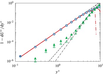
Taylor expansion of
 $(1-\text{d}U^{+}/\text{d}y^{+})$
for the DNS of Schlatter & Örlü (Reference Schlatter and Örlü2010) at
 $\mathit{Re}_{{\it\delta}_{\ast }}=5508$
: (blue) ●,
 $(1-\text{d}U^{+}/\text{d}y^{+})_{DNS}$
with fit
 $\propto (y^{+})^{3}$
(- - -); (light blue) small
 $\bullet$
,
 $\langle uv\rangle ^{+}$
from DNS; (green) ▴,
 $-(1-\text{d}U^{+}/\text{d}y^{+})_{DNS}-4t_{4}^{(U)}(y^{+})^{3}$
with fit
 $\propto (y^{+})^{5}$
(- - -); (green) ▵,
 $-(1-\text{d}U^{+}/\text{d}y^{+})_{DNS}-4t_{4}^{(U)}(y^{+})^{3}$
with different
 $t_{4}^{(U)}$
and fit
 $\propto (y^{+})^{6}$
(– ⋅ – ⋅ –); (thick red) ——, two-term Taylor expansion corresponding to
 $U^{+}=y^{+}-3.175\times 10^{-4}(y^{+})^{4}+1.917\times 10^{-6}(y^{+})^{6}$
; (thick red)
 $-\cdot -\cdot -$
, two-term Taylor expansion corresponding to
 $U^{+}=y^{+}-3.075\times 10^{-4}(y^{+})^{4}+3.429\times 10^{-7}(y^{+})^{7}$
.

In the following, the high-Reynolds-number asymptotic expansions of the Taylor series for
 $U^{+}$
,
 $V^{+}$
,
 $\langle uv\rangle ^{+}$
,
 $\langle uu\rangle ^{+}$
,
 $\langle vv\rangle ^{+}$
and
 $\langle ww\rangle ^{+}$
are extracted from the DNS. Due to the limitations of Reynolds number and numerical accuracy these Taylor series will provide good profile fits only very close to the wall, for
 $y^{+}\lesssim 8$
! Nevertheless, the conclusions will apply to the entire inner region since the form of an asymptotic expansion, i.e. the asymptotic sequence, is the same for a function and its Taylor expansion.
2.1. Determination of Taylor expansions around
$y^{+}=0$
from moderate-Re DNS

Since the fitting range of Taylor expansions is not known a priori, the following graphical procedure has been adopted. From any quantity
 $X^{+}(y^{+})$
the leading term of its Taylor expansion
 $t_{n}^{(X)}(y^{+})^{n}$
is subtracted and the coefficient
 $t_{n}^{(X)}$
is varied until the graph of the difference
 $X^{+}(y^{+})-t_{n}^{(X)}(y^{+})^{n}$
becomes a clear power law with an integer power
 $m>n$
. The procedure is repeated with increasing powers of
 $y^{+}$
until the data become too noisy. The procedure is illustrated in the following series of figures for one DNS of Schlatter & Örlü (Reference Schlatter and Örlü2010) at a Reynolds number of
 $\mathit{Re}_{{\it\delta}_{\ast }}=5508$
, corresponding to
 $U_{\infty }^{+}=25.87$
.
Figure 1 for
 $(1-\text{d}U^{+}/\text{d}y^{+})$
serves to demonstrate the difficulty of determining higher Taylor coefficients. Also included in this figure is
 $\langle uv\rangle ^{+}$
, which is almost identical to
 $(1-\text{d}U^{+}/\text{d}y^{+})$
(see, e.g., Mellor Reference Mellor1972, and § 2.2). Therefore, the coefficients of
 $(y^{+})^{2}$
and
 $(y^{+})^{3}$
in the Taylor expansion of
 $U^{+}$
must be zero, since the leading term in the expansion of
 $\langle uv\rangle ^{+}$
is
 $t_{3}^{(uv)}(y^{+})^{3}$
due to boundary conditions and continuity requiring
 $u\propto y^{+}$
and
 $v\propto (y^{+})^{2}$
near the wall. Hence,
 $$\begin{eqnarray}U^{+}=y^{+}+t_{4}^{(U)}(y^{+})^{4}+t_{n}^{(U)}(y^{+})^{n}+\cdots \,,\end{eqnarray}$$
with both
 $n=6$
and
 $n=7$
compatible with the DNS, as demonstrated in figure 1. In other words, the number of significant figures in this DNS does not allow one to unambiguously identify Taylor expansion terms of
 $U^{+}$
beyond the second term. In this case, the Taylor-expanded basic equations (see § 2.2) provide additional guidance and lead to the choice of
 $n=6$
(see table 1 for the coefficients that have been retained). However, it is clear from this fitting exercise that the uncertainty of the Taylor coefficients
 $t_{n}^{(X)}$
extracted from the computed quantity
 $X$
increases strongly with
 $n$
: while the fitting error for the leading coefficients is approximately 1 % or less for all of the quantities considered here, it rises to 10 % and more for the third coefficient. Another manifestation of the limited numerical resolution is the breakaway of the data from the higher powers for
 $y^{+}\rightarrow 0$
, most clearly seen in figures 1 and 2. It is noted in passing that in fully developed turbulent channel and pipe flows the pressure gradient modifies the Taylor series (2.1) to
 $U^{+}=y^{+}-(y^{+})^{2}/(2~{\it\delta}^{+})+\cdots \,,$
where
 ${\it\delta}$
is the channel half-height or the pipe radius. This additional quadratic term can be clearly identified in high-quality channel and pipe DNS very close to the wall and is related to the near-wall layer introduced by Klewicki and co-workers in their four-layer model (see, e.g., Klewicki Reference Klewicki2013, and references therein).
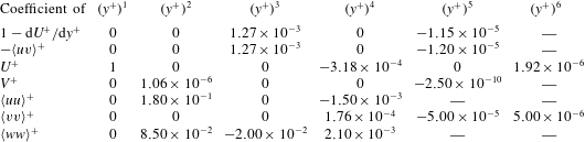
Coefficients of Taylor expansions of mean velocities and some components of the Reynolds stress tensor for the DNS of Schlatter & Örlü (Reference Schlatter and Örlü2010) at
 $\mathit{Re}_{{\it\delta}_{\ast }}=5508$
. Coefficients that cannot be resolved are identified by ‘—’.

The Taylor series for the mean wall-normal velocity
 $V^{+}$
, corresponding to the series (2.1) for
 $U^{+}$
with
 $n=6$
, is of the form
 $$\begin{eqnarray}V^{+}=t_{2}^{(V)}(y^{+})^{2}+t_{5}^{(V)}(y^{+})^{5}+\cdots \,,\end{eqnarray}$$
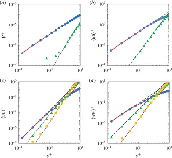
and its extraction from DNS is shown in figure 2(a) for one
 $\mathit{Re}_{{\it\delta}_{\ast }}$
. Similarly, the extraction of the Taylor expansions for
 $\langle uu\rangle ^{+}$
,
 $\langle vv\rangle ^{+}$
and
 $\langle ww\rangle ^{+}$
is shown in figure 2(b–d). No figure is shown for
 $\langle uv\rangle ^{+}$
as it would be virtually indistinguishable from figure 1. The Taylor expansion coefficients
 $t_{n}^{(uv)}$
, together with all of the other coefficients corresponding to figures 1 and 2, are summarized in table 1. Here, a remark on the missing
 $(y^{+})^{3}$
term in the Taylor expansion of
 $\langle uu\rangle ^{+}$
about
 $y^{+}=0$
is warranted. This term must be zero to ensure compatibility with the Taylor expansion of
 $\langle {\it\omega}_{z}{\it\omega}_{z}\rangle ^{+}$
, where
 ${\it\omega}_{z}$
is the fluctuating transverse vorticity, which is of the form
 $\langle {\it\omega}_{z}{\it\omega}_{z}\rangle ^{+}=t_{0}^{({\it\omega}_{z}{\it\omega}_{z})}+t_{2}^{({\it\omega}_{z}{\it\omega}_{z})}(y^{+})^{2}+\cdots \,$
(see, e.g., Kim & Adrian Reference Kim and Adrian1999; Panton Reference Panton2009; Schlatter & Örlü Reference Schlatter and Örlü2010). Since
 $\langle {\it\omega}_{z}{\it\omega}_{z}\rangle$
can be decomposed into
 $\langle (\partial v/\partial x)^{2}\rangle +\langle (\partial u/\partial y)^{2}\rangle -2\langle (\partial v/\partial x)(\partial u/\partial y)\rangle$
, it follows not only that
 $t_{3}^{(uu)}=0$
, but also that the Taylor coefficients
 $t_{0}^{({\it\omega}_{z}{\it\omega}_{z})}$
and
 $t_{2}^{(uu)}$
are identical (this is confirmed by the DNS of Schlatter & Örlü (Reference Schlatter and Örlü2010) with less than 1 % error).
Taylor expansions of (a)
 $V^{+}=t_{2}^{(V)}(y^{+})^{2}+t_{5}^{(V)}(y^{+})^{5}$
, (b)
 $\langle uu\rangle ^{+}=t_{2}^{(uu)}(y^{+})^{2}+t_{4}^{(uu)}(y^{+})^{4}$
, (c)
 $\langle vv\rangle ^{+}=t_{4}^{(vv)}(y^{+})^{4}+t_{5}^{(vv)}(y^{+})^{5}+t_{6}^{(vv)}(y^{+})^{6}$
and (d)
 $\langle ww\rangle ^{+}=t_{2}^{(ww)}(y^{+})^{2}+t_{3}^{(ww)}(y^{+})^{3}+t_{4}^{(ww)}(y^{+})^{4}$
from the DNS of Schlatter & Örlü (Reference Schlatter and Örlü2010) at
 $\mathit{Re}_{{\it\delta}_{\ast }}=5508$
. See table 1 for coefficient values and figure 1 for symbols.

2.2. The balance of the Taylor-expanded momentum equation at large Reynolds numbers
In the following, the Taylor expansions of mean velocities and stresses over the available range of DNS Reynolds numbers, determined according to the procedure outlined in the previous § 2.1, are used to verify the large-Reynolds-number asymptotic expansion of the streamwise momentum equation
 $$\begin{eqnarray}U\,\frac{\partial U}{\partial x}+V\,\frac{\partial U}{\partial y}={\it\nu}~\frac{\partial ^{2}U}{\partial y^{2}}-\frac{\partial \langle uv\rangle }{\partial y}-\frac{\partial }{\partial x}\,\left[\langle uu\rangle -\langle vv\rangle \right]\end{eqnarray}$$
close to the wall, where it can be Taylor expanded (see appendix B for the underlying assumptions and a detailed derivation). For this, the streamwise derivatives in (2.3) need to be evaluated. To simplify the presentation, the small parameter
 $(1/U_{\infty }^{+})$
is abbreviated in the following as
 $$\begin{eqnarray}{\it\epsilon}\equiv \frac{1}{U_{\infty }^{+}},\end{eqnarray}$$
while no shorthand is used for the second small parameter
 $(1/\mathit{Re}_{{\it\delta}_{\ast }})$
in order to avoid confusion. In terms of
 ${\it\epsilon}$
, the asymptotic expansions of the streamwise derivatives of
 $U_{\infty }^{+}$
and
 ${\it\delta}_{\ast }$
, developed in appendix B (B 14) and (B 15), take the form
 $$\begin{eqnarray}\frac{\text{d}U_{\infty }^{+}}{\text{d}x}=\frac{{\it\epsilon}^{2}}{{\it\kappa}{\it\delta}_{\ast }}\,\mathscr{X}({\it\epsilon})+\mathscr{B}\mathit{O}\left(\mathit{Re}_{{\it\delta}_{\ast }}\right)^{-1}\quad \text{and}\quad \frac{\text{d}{\it\delta}_{\ast }}{\text{d}x}={\it\epsilon}^{2}\,\widetilde{\mathscr{X}}({\it\epsilon})+\mathscr{B}\mathit{O}\left(\mathit{Re}_{{\it\delta}_{\ast }}\right)^{-1},\end{eqnarray}$$
where
 ${\it\kappa}$
is the Kármán constant and
 ${\mathcal{B}}$
designates ‘block order’, defined after (B 9). The functions
 $\mathscr{X}$
and
 $\widetilde{\mathscr{X}}$
have the asymptotic expansions
 $$\begin{eqnarray}\displaystyle \mathscr{X}\sim 1+{\it\epsilon}\,\mathscr{X}_{1}+\mathit{O}\left({\it\epsilon}^{2}\right),\quad \widetilde{\mathscr{X}}\sim 1+{\it\epsilon}\,\widetilde{\mathscr{X}}_{1}+\mathit{O}\left({\it\epsilon}^{2}\right),\quad \text{with}~\mathscr{X}_{1}=\widetilde{\mathscr{X}}_{1}=I_{\mathit{ww}}^{(0)}+I_{\mathit{nsd}}^{(0)}, & & \displaystyle \nonumber\\ \displaystyle & & \displaystyle\end{eqnarray}$$
where
 $I_{\mathit{ww}}^{(0)}$
and
 $I_{\mathit{nsd}}^{(0)}$
are defined in (B 12a,b
). It should be noted that we have used the
 $x$
derivative (B 15) of
 ${\it\delta}_{\ast }$
in anticipation of the result that the Taylor-expanded momentum equation can only be balanced if the normal stresses are scaled with
 $u_{{\it\tau}}^{2}$
.
Starting with the continuity equation, table 1 and the analogous reduction of the 12 other DNS data sets, the coefficients of the Taylor expansion (2.1) of
 $U^{+}$
are obtained as functions of
 ${\it\epsilon}\equiv (1/U_{\infty }^{+})$
and/or
 $(1/\mathit{Re}_{{\it\delta}_{\ast }})$
. By rewriting the Taylor expansion in terms of the
 $x$
-independent coordinate
 $\breve{y}\equiv yU_{\infty }/{\it\nu}=y^{+}/{\it\epsilon}$
, the
 $x$
dependence of
 $U$
is contained exclusively in
 ${\it\epsilon}(x)$
:
 $$\begin{eqnarray}U=U_{\infty }\left\{{\it\epsilon}^{2}\breve{y}+{\it\epsilon}^{5}t_{4}^{(U)}\breve{y}^{4}+\cdots \hspace{-1.3pt}\right\}\hspace{-0.8pt}.\end{eqnarray}$$
With (2.6a,b
) the
 $x$
derivative of
 $U$
is easily obtained. After replacing
 ${\it\epsilon}\breve{y}$
by
 $y^{+}$
, one has
 $$\begin{eqnarray}\frac{\partial U}{\partial x}=-\frac{\partial V}{\partial y}=-{\it\epsilon}^{4}\,\frac{U_{\infty }~\mathscr{X}({\it\epsilon})}{{\it\kappa}{\it\delta}_{\ast }}\left\{2\,y^{+}+5\,t_{4}^{(U)}\,(y^{+})^{4}+\cdots \hspace{-1.3pt}\right\}\hspace{-0.8pt}.\end{eqnarray}$$
Integrating with respect to
 $y$
and regrouping yields
 $$\begin{eqnarray}V^{+}=\frac{{\it\epsilon}^{2}}{\mathit{Re}_{{\it\delta}_{\ast }}}\frac{\mathscr{X}({\it\epsilon})}{{\it\kappa}}\left\{(y^{+})^{2}+t_{4}^{(U)}(y^{+})^{5}+\cdots \hspace{-1.3pt}\right\}\hspace{-0.8pt}.\end{eqnarray}$$
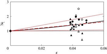
The function
 $\mathscr{X}({\it\epsilon})$
obtained by comparing the first two terms of the Taylor expansion of
 $V^{+}$
extracted from DNS with the corresponding terms in (2.9) derived from the Taylor expansion of
 $U^{+}$
: ●, ○ , from coefficient of
 $(y^{+})^{2}$
; ▴, ▵, from coefficient of
 $(y^{+})^{5}$
; ♦ , theoretical infinite-Reynolds-number limit
 $\mathscr{X}({\it\epsilon}=0)\equiv 1$
;
 $-~-~-$
(red), linear least-squares fit
 $\mathscr{X}=1+10.4\,{\it\epsilon}$
of all the data points
 $\pm$
one standard deviation
 ${\it\sigma}=9.2\,{\it\epsilon}$
(red
 $\cdots \cdots$
); —— (black), quadratic least-squares fit
 $\mathscr{X}=1+7.4\,{\it\epsilon}+68\,{\it\epsilon}^{2}$
with linear term taken from (2.6a,b
) with
 $I_{\mathit{ww}}^{(0)}=7.11$
and
 $I_{\mathit{nsd}}^{(0)}=0.3$
. The solid and open symbols correspond to DNS by Schlatter & Örlü (Reference Schlatter and Örlü2010) and Jimenez et al. (Reference Jimenez, Hoyas, Simens and Mizuno2010) respectively.

By comparing the fitted Taylor coefficients of
 $V^{+}$
with (2.9), it is straightforward to determine the function
 $\mathscr{X}\left({\it\epsilon}\right)$
. The result is shown in figure 3 for the first two terms of (2.9), and it is obvious that the accuracy of both our method to extract Taylor expansions from the DNS and of the DNS itself is insufficient to obtain a reliable value for the coefficient
 $\mathscr{X}_{1}$
of
 ${\it\epsilon}$
in (2.6a,b
). This is in large part due to the fact that close to the wall the two dominant terms in the momentum balance, viscous and Reynolds stress, nearly cancel, as seen, for instance, from the Taylor coefficients in table 1 (see also Mellor Reference Mellor1972). To avoid the uncertainty in
 $\mathscr{X}$
, the complete Taylor-expanded momentum balance is not verified at individual Reynolds numbers, but the ensemble of available DNS is used to determine the asymptotic expansion of each Taylor coefficient, involving its extrapolation to infinite Reynolds number. Limitation to the first few terms of the double Taylor/asymptotic expansion of the momentum equation (2.3) requiring only the exact leading behaviour
 $\mathscr{X}\sim \widetilde{\mathscr{X}}\sim 1$
in (2.5a,b
) will allow us to demonstrate that a balance is only possible if the near-wall normal Reynolds stresses are inner scaled with
 $u_{{\it\tau}}^{2}$
.
Before proceeding with the above programme, some useful conclusions can nevertheless be drawn from figure 3. First, the data scatter in figure 3 cannot be attributed solely to a loss of significant digits of
 $V^{+}$
. If in figure 2(a) the deviation of the computed
 $V^{+}$
from its two-term Taylor expansion below
 $y^{+}\approx 2$
is taken as an indicator,
 $V^{+}$
has at least two significant digits down to
 $y^{+}\approx 1$
. Hence, the large standard deviation of the least-squares linear fit
 $\text{d}\mathscr{X}/\text{d}{\it\epsilon}=10.4\pm 9.2$
in figure 3 must also be due to differences in tripping and boundary conditions between the individual DNS runs, as discussed by Schlatter & Örlü (Reference Schlatter and Örlü2013). Second, the data of figure 3 are found to be nearly randomly scattered around the two-term expansion (2.6a,b
) of
 $\mathscr{X}$
obtained directly from the integrated momentum equation in appendix B. With
 $I_{\mathit{ww}}^{(0)}=7.11$
taken from MCN07 and
 $I_{\mathit{nsd}}^{(0)}\approx 0.3$
, chosen somewhat smaller than
 $\int \langle uu\rangle ^{+}({\it\epsilon}=0)\,\text{d}Y=0.39$
obtained from the fit (4.10), one obtains a slope of 7.4, only
 ${\it\sigma}/3$
below the least-squares slope of 10.4. This suggests that the next
 ${\it\epsilon}^{2}$
term in the asymptotic expansion of
 $\mathscr{X}$
is small or possibly even zero: a quadratic least-squares fit with the linear coefficient fixed to 7.4 yields
 $\mathscr{X}=1+7.4\,{\it\epsilon}+68\,{\it\epsilon}^{2}$
, which is seen in figure 3 to deviate little from the linear fit.
We now focus attention on the first two terms
 $\propto (y^{+})^{2}$
and
 $\propto (y^{+})^{4}$
of the Taylor-expanded momentum balance. The left-hand side of (2.3) is obtained from (2.7)–(2.9) as
 $$\begin{eqnarray}U\frac{\partial U}{\partial x}+V\frac{\partial U}{\partial y}=-\frac{u_{{\it\tau}}^{3}}{{\it\nu}}\frac{{\it\epsilon}^{2}}{\mathit{Re}_{{\it\delta}_{\ast }}}~\frac{\mathscr{X}({\it\epsilon})}{{\it\kappa}}\left\{(y^{+})^{2}+\text{coef.}\,(y^{+})^{5}+\cdots \hspace{-1.3pt}\right\}.\end{eqnarray}$$
It should be noted that the coefficient of
 $(y^{+})^{2}$
in (2.10) does not require any data fitting but contains the function
 $\mathscr{X}({\it\epsilon})$
. As outlined above, the analysis will therefore be limited to the order
 $\mathit{O}({\it\epsilon}^{2}/\mathit{Re}_{{\it\delta}_{\ast }})$
to avoid the large uncertainty of
 $\mathscr{X}_{1}$
in the expansion (2.6a,b
). It is also noted that the Taylor coefficients of
 $(y^{+})^{3}$
and
 $(y^{+})^{4}$
in (2.10) are zero due to the structure of the Taylor expansion of
 $U$
(see § 2.1).
The scaling of the left-hand side of (2.10) near the wall implies that the corrections to the leading-order inner balance between viscous and Reynolds stresses are of order
 $(u_{{\it\tau}}^{3}/{\it\nu})~({\it\epsilon}^{2}/\mathit{Re}_{{\it\delta}_{\ast }})$
, where the factor
 $(u_{{\it\tau}}^{3}/{\it\nu})$
is the dimensional reference quantity for (2.10). Hence, the Taylor series of
 $U^{+}$
and
 $-\langle uv\rangle ^{+}$
must have the asymptotic expansions
 $$\begin{eqnarray}\displaystyle & U^{+}=y^{+}+t_{4}^{(U)}(y^{+})^{4}+t_{6}^{(U)}(y^{+})^{6}+\cdots \,,\quad \text{with }t_{i}^{(U)}=t_{i,0}^{(U)}+\displaystyle \frac{{\it\epsilon}^{2}}{\mathit{Re}_{{\it\delta}_{\ast }}}\,t_{i,1}^{(U)}+\mathit{O}\left(\frac{{\it\epsilon}^{3}}{\mathit{Re}_{{\it\delta}_{\ast }}}\right), & \displaystyle \nonumber\\ \displaystyle & & \displaystyle\end{eqnarray}$$
 $$\begin{eqnarray}\displaystyle & -\langle uv\rangle ^{+}=t_{3}^{(uv)}(y^{+})^{3}+t_{5}^{(uv)}(y^{+})^{5}+\cdots \,,\quad \text{with }t_{i}^{(uv)}=t_{i,0}^{(uv)}+\displaystyle \frac{{\it\epsilon}^{2}}{\mathit{Re}_{{\it\delta}_{\ast }}}\,t_{i,1}^{(uv)}+\mathit{O}\left(\frac{{\it\epsilon}^{3}}{\mathit{Re}_{{\it\delta}_{\ast }}}\right). & \displaystyle \nonumber\\ \displaystyle & & \displaystyle\end{eqnarray}$$
As will become evident from the balancing of (2.3), the Taylor series of the normal stresses must have the asymptotic expansions
 $$\begin{eqnarray}\displaystyle & \hspace{-12.0pt}\langle uu\rangle ^{+}=t_{2}^{(uu)}(y^{+})^{2}+t_{4}^{(uu)}(y^{+})^{4}+\cdots \,,\quad \text{with }t_{i}^{(uu)}=t_{i,0}^{(uu)}+{\it\epsilon}\,t_{i,1}^{(uu)}+\mathit{O}\left({\it\epsilon}^{2}\right), & \displaystyle\end{eqnarray}$$
 $$\begin{eqnarray}\displaystyle & \hspace{-12.0pt}\langle vv\rangle ^{+}=t_{4}^{(vv)}(y^{+})^{4}+t_{5}^{(ww)}(y^{+})^{5}+\cdots \,,\quad \text{with }t_{i}^{(vv)}=t_{i,0}^{(vv)}+{\it\epsilon}\,t_{i,1}^{(vv)}+\mathit{O}\left({\it\epsilon}^{2}\right), & \displaystyle\end{eqnarray}$$
 $$\begin{eqnarray}\displaystyle & \hspace{-12.0pt}\langle ww\rangle ^{+}=t_{2}^{(ww)}(y^{+})^{2}+t_{3}^{(ww)}(y^{+})^{3}+\cdots \,,\quad \text{with }t_{i}^{(ww)}=t_{i,0}^{(ww)}+{\it\epsilon}\,t_{i,1}^{(ww)}+\mathit{O}\left({\it\epsilon}^{2}\right), & \displaystyle\end{eqnarray}$$
where the spanwise stress, not needed for the momentum balance, has been added for completeness.
The
 $y$
derivatives of the Taylor expansions (2.11) of
 $U^{+}$
and (2.12) of
 $-\langle uv\rangle ^{+}$
are easily evaluated. For the
 $x$
derivatives of the Taylor expansions (2.13) of
 $\langle uu\rangle ^{+}$
and (2.14) of
 $\langle vv\rangle ^{+}$
, on the other hand, the
 $x$
-independent coordinate
 $\breve{y}\equiv yU_{\infty }/{\it\nu}=y^{+}/{\it\epsilon}$
has to be introduced temporarily as in (2.7), to use (2.5a,b
) for the
 $x$
derivative of
 ${\it\epsilon}$
. With (2.5a,b
), (2.13) and (2.14) the
 $x$
derivative of the normal stress difference is
 $$\begin{eqnarray}\displaystyle & & \displaystyle -\frac{\partial \langle uu\rangle }{\partial x}+\frac{\partial \langle vv\rangle }{\partial x}\sim \frac{u_{{\it\tau}}^{3}}{{\it\nu}}\frac{{\it\epsilon}^{2}}{\mathit{Re}_{{\it\delta}_{\ast }}}\frac{1}{{\it\kappa}}\nonumber\\ \displaystyle & & \displaystyle \quad \times \,\left\{\left[4\,t_{2,0}^{(uu)}+\mathit{O}({\it\epsilon})\right](y^{+})^{2}+\left[6\,t_{4,0}^{(uu)}-6\,t_{4,0}^{(vv)}+\mathit{O}({\it\epsilon})\right](y^{+})^{4}+\cdots \hspace{-1.0pt}\right\}.\end{eqnarray}$$
This finally allows us to check the coefficients of
 $(y^{+})^{2}$
and
 $(y^{+})^{4}$
in the Taylor expansion of the momentum equation (2.3) up to order
 $\mathit{O}({\it\epsilon}^{2}/\mathit{Re}_{{\it\delta}_{\ast }})$
. With (2.10), the
 $y$
derivatives of (2.11) and (2.12), and (2.16) one obtains respectively
 $$\begin{eqnarray}\displaystyle & \hspace{-18.0pt}\displaystyle -\frac{{\it\epsilon}^{2}}{\mathit{Re}_{{\it\delta}_{\ast }}}\frac{1}{{\it\kappa}}=\left[12\,t_{4,0}^{(U)}+3\,t_{3,0}^{(uv)}\right]+\frac{{\it\epsilon}^{2}}{\mathit{Re}_{{\it\delta}_{\ast }}}~\left[12\,t_{4,1}^{(U)}+3\,t_{3,1}^{(uv)}+\frac{4}{{\it\kappa}}t_{2,0}^{(uu)}\right]+\mathit{O}\left(\frac{{\it\epsilon}^{3}}{\mathit{Re}_{{\it\delta}_{\ast }}}\right), & \displaystyle\end{eqnarray}$$
 $$\begin{eqnarray}\displaystyle & \hspace{-18.0pt}\displaystyle 0=\left[30\,t_{6,0}^{(U)}+5\,t_{5,0}^{(uv)}\right]+\frac{{\it\epsilon}^{2}}{\mathit{Re}_{{\it\delta}_{\ast }}}\left[30\,t_{6,1}^{(U)}+5\,t_{5,1}^{(uv)}+\frac{6}{{\it\kappa}}\left(t_{4,0}^{(uu)}-t_{4,0}^{(vv)}\right)\right]+\mathit{O}\left(\frac{{\it\epsilon}^{3}}{\mathit{Re}_{{\it\delta}_{\ast }}}\right)\!. & \displaystyle\end{eqnarray}$$
It should be noted that the neglected terms of
 $\mathit{O}({\it\epsilon}^{3}/\mathit{Re}_{{\it\delta}_{\ast }})$
in (2.17) and (2.18) contain the second terms of the expansions (2.6a,b
) of
 $\mathscr{X}$
and
 $\widetilde{\mathscr{X}}$
as well as the third terms of the asymptotic expansions of
 $t_{4}^{(U)}$
,
 $t_{3}^{(uv)}$
, etc., which cannot be reliably determined from the present DNS data. In addition, the
 $x$
derivative of
 $\langle uv\rangle$
, neglected in the
 $y$
momentum equation (B 1), also contributes to the order
 $\mathit{O}({\it\epsilon}^{3}/\mathit{Re}_{{\it\delta}_{\ast }})$
. Equations (2.17) and (2.18) represent four constraints on the 11 coefficients they relate. The two constraints at
 $\mathit{O}(1)$
relate the infinite-Reynolds-number limits
 $t_{3,0}^{(uv)}$
to
 $t_{4,0}^{(U)}$
and
 $t_{5,0}^{(uv)}$
to
 $t_{6,0}^{(U)}$
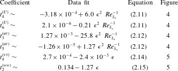
. The seven coefficients determined from the Taylor series fitted to DNS over a range of Reynolds numbers and the two coefficients
 $t_{3,0}^{(uv)}$
and
 $t_{5,0}^{(uv)}$
obtained from the two
 $\mathit{O}(1)$
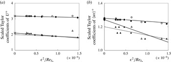
constraints are summarized in table 2. As seen in figure 4, the first of these constraints is very well satisfied, and the infinite-Reynolds-number limit
 $-t_{5,0}^{(uv)}=1.26\times 10^{-5}$
is only 5 % above the least-squares fit through the data, shown as a dotted line in figure 4(b).
(a) Scaled coefficients
 $-t_{4}^{(U)}\times 10^{4}$
(●, ○) and
 $t_{6}^{(U)}\times 10^{6}$
(▴, ▵) of the Taylor expansion of
 $U^{+}$
versus
 $({\it\epsilon}^{2}/\mathit{Re}_{{\it\delta}_{\ast }})$
;
 $\times$
, extrapolation of DNS data to infinite
 $\mathit{Re}$
. (b) Scaled coefficients
 $t_{3}^{(uv)}\times 10^{3}$
(●, ○) and
 $-t_{5}^{(uv)}\times 10^{5}$
(▴, ▵) of the Taylor expansion of
 $-\langle uv\rangle ^{+}$
versus
 $({\it\epsilon}^{2}/\mathit{Re}_{{\it\delta}_{\ast }})$
; —— , linear fits of table 2; ♦ , infinite-
 $\mathit{Re}$
limit obtained from the leading-order balance of (2.17) and (2.18);
 $\cdots \cdots$
, alternate fits based on the least-squares fit of
 $t_{5}^{(uv)}$
described in the text. See figure 3 for further explanation of the symbols.

Asymptotic expansion of leading Taylor coefficients of
 $U^{+}$
and some components of the Reynolds stress tensor extracted from the DNS of Schlatter & Örlü (Reference Schlatter and Örlü2010) satisfying the constraints (2.17) and (2.18).

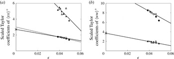
(a) Scaled coefficients
 $t_{4}^{(vv)}\times 10^{4}$
(●, ○) and
 $-t_{5}^{(vv)}\times 10^{5}$
(▴, ▵) of the Taylor expansion of
 $\langle vv\rangle ^{+}$
versus
 $(1/U_{\infty }^{+})$
. (b) Scaled coefficients
 $t_{2}^{(ww)}\times 10^{2}$
(●, ○) and
 $-t_{3}^{(ww)}\times 10^{2}$
(▴, ▵) of the Taylor expansion of
 $\langle ww\rangle ^{+}$
versus
 $(1/U_{\infty }^{+})$
; —— , linear fits of table 2;
 $\cdots \cdots$
, alternate fit based on the least-squares fit of
 $t_{5}^{(uv)}$
. See figures 3 and 4 for further explanation of the symbols.

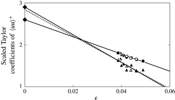
Scaled coefficients
 $t_{2}^{(uu)}\times 10$
(●, ○) and
 $-t_{4}^{(uu)}\times 10^{3}$
(▴, ▵) of the Taylor expansion of
 $\langle uu\rangle ^{+}$
versus
 ${\it\epsilon}$
; ♦ , infinite-
 $\mathit{Re}$
limit obtained from the balance of (2.17) and (2.18) at
 $\mathit{O}({\it\epsilon}^{2}/\mathit{Re}_{{\it\delta}^{\ast }})$
;
 $\cdots \cdots$
, alternate fit based on the least-squares fit of
 $t_{5}^{(uv)}$
. See figure 3 for further explanation of the symbols.

At this point, the remaining two constraints of (2.17) and (2.18) at order
 $\mathit{O}({\it\epsilon}^{2}/\mathit{Re}_{{\it\delta}^{\ast }})$
allow linking of the infinite-Reynolds-number limits
 $t_{2,0}^{(uu)}$
and
 $t_{4,0}^{(uu)}$
to the fitted slopes in figure 4 and to the infinite-Reynolds-number limit
 $t_{4,0}^{(vv)}$
in figure 5 (see table 2). With
 ${\it\kappa}=0.384$
one obtains
 $$\begin{eqnarray}\displaystyle & t_{2}^{(uu)}=0.26-2.05\,{\it\epsilon}+\mathit{O}({\it\epsilon}^{2}), & \displaystyle\end{eqnarray}$$
 $$\begin{eqnarray}\displaystyle & t_{4}^{(uu)}=-0.0029+0.033\,{\it\epsilon}+\mathit{O}({\it\epsilon}^{2}), & \displaystyle\end{eqnarray}$$
where the coefficients of
 ${\it\epsilon}$
in (2.19) and (2.20) are best fits through the respective infinite-Reynolds-number limits and the data. As seen in figure 6, these infinite-Reynolds-number limits deduced from the momentum balance match up nicely with the linear extension of the data extracted from DNS, despite their relatively low Reynolds numbers.
To obtain a feeling for the uncertainty of the fits in table 2, the consequences of replacing
 $t_{5}^{(uv)}$
by the least-squares data fit are explored. The latter corresponds to
 $t_{5,0}^{(uv)}=-1.20\times 10^{-5}$
(
 $+$
5 % relative to table 2) and
 $t_{5,1}^{(uv)}=0.71$
(
 $-$
44 % relative to table 2). To satisfy the leading-order constraint (2.18),
 $t_{6,0}^{(U)}$
has to be decreased by 5 % to
 $2.0\times 10^{-6}$
. At order
 ${\it\epsilon}^{2}/\mathit{Re}_{{\it\delta}_{\ast }}$
, the modification of
 $t_{5,1}^{(uv)}$
entrains modifications of the other three coefficients to
 $t_{6,1}^{(U)}=-0.12$
(
 $+$
44 % relative to table 2),
 $t_{4,0}^{(uu)}=-0.00284$
(
 $+$
2 %) and
 $t_{4,0}^{(vv)}=3\times 10^{-4}$
(
 $+$
11 %), which have been optimized to provide the best combination of data fits and are included as dotted lines in figures 5(a) and 6. As the data scatter of
 $t_{6,0}^{(U)}$
in figure 4(a) is significantly smaller than that of
 $t_{5}^{(uv)}$
in (b), the fits of table 2 will be used in the following.
This ‘balancing act’ inspires confidence in our extrapolation of the DNS set of near-wall velocities and Reynolds stress components to infinite Reynolds number. Conversely, the successful balancing of the terms in (2.17) and (2.18), which are of
 $\mathit{O}({\it\epsilon}^{2}/\mathit{Re}_{{\it\delta}_{\ast }})$
relative to the dominant terms
 $\text{d}^{2}U^{+}/(\text{d}y^{+})^{2}$
and
 $-\text{d}\langle uv\rangle ^{+}/\text{d}y^{+}$
, also inspires confidence in the DNS.
2.3. Key results of § 2
Finite-Reynolds-number corrections to
 $U^{+}$
and
 $\langle uv\rangle ^{+}$
: the corrections to the leading-order Taylor expansions of
 $U^{+}$
and
 $\langle uv\rangle ^{+}$
are of order
 $\mathit{O}({\it\epsilon}^{2}/\mathit{Re}_{{\it\delta}_{\ast }})$
, the same order as the convective terms. As evidenced by the excellent linear fits in figure 4, the next term
 $\propto ({\it\epsilon}^{3}/\mathit{Re}_{{\it\delta}_{\ast }})$
is either zero or very small.
The inner streamwise normal stress scales with
 $u_{{\it\tau}}^{2}$
: if
 $\langle uu\rangle _{\mathit{inner}}$
did scale as
 $u_{{\it\tau}}U_{\infty }$
, the term
 $t_{2,0}^{(uu)}$
would move up to
 $\mathit{O}({\it\epsilon}/\mathit{Re}_{{\it\delta}_{\ast }})$
in (2.17), where it cannot be balanced by the
 $\mathit{O}({\it\epsilon}^{2}/\mathit{Re}_{{\it\delta}_{\ast }})$
corrections to
 $U^{+}$
and
 $\langle uv\rangle ^{+}$
, independently of the coefficient value
 $t_{2,0}^{(uu)}$
. Therefore, the Taylor coefficients of
 $\langle uu\rangle _{\mathit{inner}}^{+}$
are finite in the limit of infinite Reynolds number.
Asymptotic expansion of near-wall normal stresses: the asymptotic expansion of the Taylor-expanded near-wall normal stresses is of the form
 $\langle \cdot \,\cdot \rangle _{\mathit{inner}}^{+}\sim \langle \cdot \,\cdot \rangle _{0}^{+}+{\it\epsilon}\,\langle \cdot \,\cdot \rangle _{1}^{+}+\mathit{O}({\it\epsilon}^{2})$
, where the quadratic term is small or possibly zero, as evidenced by figures 5 and 6.
Finally, since an asymptotic sequence does not change when a function is Taylor expanded, the above conclusions on the form of the various asymptotic expansions remain valid for the non-expanded inner flow variables. This firmly establishes the inner scaling of
 $\langle uu\rangle _{\mathit{inner}}^{+}(y^{+})$
, as well as its asymptotic expansion which must be of the form
 $$\begin{eqnarray}\langle uu\rangle _{\mathit{inner}}^{+}\sim \langle uu\rangle _{0}^{+}(y^{+})+{\it\epsilon}\,\langle uu\rangle _{1}^{+}(y^{+})+\mathit{O}({\it\epsilon}^{2}).\end{eqnarray}$$
This implies, in particular, that the near-wall peak of
 $\langle uu\rangle ^{+}$
at
 $y^{+}\approx 15$
remains finite in the limit of infinite Reynolds number (see § 4 and figure 12).
3. Estimating the extent and slope of the logarithmic region of
$\langle uu\rangle ^{+}$

After establishing the scaling of
 $\langle uu\rangle _{\mathit{inner}}$
with
 $u_{{\it\tau}}^{2}$
and its asymptotic expansion (2.21) in the inner region, it is worthwhile to investigate the constraints on the matching to the outer
 $\langle uu\rangle _{\mathit{outer}}^{+}$
. Experimentally, the outer profile has been found to decrease logarithmically towards the free stream, and the logarithmic slope has been suggested to be a universal constant for all three ‘canonical’ wall-bounded flows, i.e. ZPG TBL, pipe and channel flows (see, e.g., Marusic et al.
Reference Marusic, Monty, Hultmark and Smits2013, and references therein).
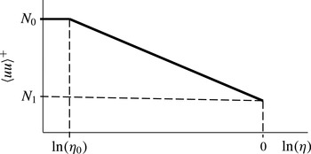
For the following, we assume a simplified profile for
 $\langle uu\rangle ^{+}$
, shown in figure 7 and given by
 $$\begin{eqnarray}\langle uu\rangle ^{+}=\left\{\begin{array}{@{}ll@{}}N_{0},\quad & \text{for}~{\it\eta}<{\it\eta}_{0},\\ N_{1}+\displaystyle \frac{N_{0}-N_{1}}{\ln ({\it\eta}_{0})}\ln ({\it\eta}),\quad & \text{for}~{\it\eta}\geqslant {\it\eta}_{0},\end{array}\right.\end{eqnarray}$$
in terms of the outer non-dimensional wall-normal coordinate
 ${\it\eta}\equiv y^{+}/\mathit{Re}_{{\it\tau}}$
ranging from zero to unity for all three ‘canonical’ flows. Here,
 $\mathit{Re}_{{\it\tau}}\equiv u_{{\it\tau}}{\it\delta}/{\it\nu}$
, with the reference length
 ${\it\delta}$
equal to the channel half-height, pipe radius or ZPG TBL boundary layer thickness respectively. In the ZPG TBL
 $\mathit{Re}_{{\it\tau}}\approx 0.24\,\mathit{Re}_{{\it\delta}_{\ast }}$
since the boundary layer edge is located at
 $Y\equiv y^{+}/\mathit{Re}_{{\it\delta}_{\ast }}\approx 0.24$
. Since we are only interested in the scaling of the breakpoint
 ${\it\eta}_{0}$
and of the logarithmic slope, the inner part of
 $\langle uu\rangle ^{+}$
in the interval
 $0\leqslant {\it\eta}<{\it\eta}_{0}$
, including the rise from the wall to the inner peak at
 $y^{+}\approx 15$
and the connection to the second maximum or plateau, may be radically simplified by extending the level
 $N_{0}$
to
 ${\it\eta}=0$
, with
 $N_{0}=\mathit{O}(1)$
, as demonstrated in the previous § 2.
Schematic of the
 $\langle uu\rangle ^{+}$
profile for all three canonical flows.

3.1. A geometric argument for a Reynolds-number-dependent logarithmic slope
Here, the most general
 $\mathit{Re}_{{\it\tau}}$
dependence of the breakpoint
 ${\it\eta}_{0}=(c\,{\it\mu}^{n}\,\mathit{Re}_{{\it\tau}}^{m})^{-1}$
is assumed, where
 ${\it\mu}\equiv 1/\ln (\mathit{Re}_{{\it\tau}})$
and
 $n=0$
,
 $m=1$
correspond to a constant
 ${\it\eta}_{0}^{+}\equiv {\it\eta}_{0}/\mathit{Re}_{{\it\tau}}$
. Connecting the two points
 $({\it\eta},\langle uu\rangle ^{+})=({\it\eta}_{0},N_{0})$
and
 $(1,N_{1})$
by a logarithm trivially leads to
 $$\begin{eqnarray}\langle uu\rangle ^{+}=N_{1}-\frac{N_{0}-N_{1}}{\ln (c{\it\mu}^{n}\,\mathit{Re}_{{\it\tau}}^{m})}\ln ({\it\eta}).\end{eqnarray}$$
One way for the slope in (3.2) to become constant is to set
 $n=m=0$
, i.e. to have the start of the logarithmic decay scale with
 ${\it\delta}$
, which is at odds with all available data. When
 $n$
and/or
 $m$
in (3.2) are/is different from zero, a constant logarithmic slope is only possible if
 $N_{0}$
scales as
 $\ln ({\it\mu}^{n}\,\mathit{Re}_{{\it\tau}}^{m})$
, which violates the scaling of
 $\langle uu\rangle _{\mathit{inner}}^{+}\sim \mathit{O}(1)$
demonstrated in § 2.
An alternative more physical way to show that the logarithmic slope between
 ${\it\eta}_{0}$
and
 ${\it\eta}=1$
in figure 7 cannot be constant can be derived from a simplified balance of turbulence energy production
 $P$
and dissipation
 $D$
.
3.2. Estimates based on turbulence energy production and dissipation
The geometric argument of § 3.1 is complemented by a simplified consideration of the turbulent energy balance, which will yield
 $n=m=1$
for the exponents in (3.2).
The dominant production term for turbulent kinetic energy is
 $$\begin{eqnarray}P=-\frac{u_{{\it\tau}}^{4}}{{\it\nu}}\,\langle uv\rangle ^{+}\frac{\partial U^{+}}{\partial y^{+}}.\end{eqnarray}$$
For the inner part we use the rough approximations
 $(\partial U^{+}/\partial y^{+})=1$
up to
 $y^{+}=1/{\it\kappa}$
and
 $(\partial U^{+}/\partial y^{+})=1/({\it\kappa}y^{+})$
beyond, while
 $\langle uv\rangle ^{+}$
is taken to be
 $t_{3}^{(uv)}(y^{+})^{3}$
up to
 $y^{+}=(t_{3}^{(uv)})^{-1/3}$
and unity beyond. For the outer part,
 $(\partial U^{+}/\partial y^{+})\sim \mathit{Re}_{{\it\tau}}^{-1}\,[({\it\kappa}{\it\eta})^{-1}-F^{\prime }({\it\eta})]$
, with
 $F$
describing the smooth transition from the log law to
 $(\partial U^{+}/\partial {\it\eta})({\it\eta}=1)=0$
. The outer Reynolds stress is approximated by
 $\langle uv\rangle ^{+}\approx 1-{\it\eta}$
. The resulting estimate of production, integrated over the entire TBL, is
 $$\begin{eqnarray}\int _{0}^{{\it\delta}}P\,\text{d}y=u_{{\it\tau}}^{3}\,\left[\frac{1}{{\it\kappa}}\ln (\mathit{Re}_{{\it\tau}})+\text{const.}\right]\end{eqnarray}$$
and has the standard logarithmic dependence on Reynolds number (see, e.g., Laadhari Reference Laadhari2007).
To relate the scaling of the dissipation at the wall distance
 $y$
to the scaling of
 $\langle uu\rangle$
, we make the rather drastic simplification of taking the turbulent kinetic energy
 $K$
proportional to
 $\langle uu\rangle$
. This implies that all three normal stresses have the same Reynolds number scaling and that turbulent convection and interscale fluxes are of secondary importance for the Reynolds number scaling of the integrated dissipation. Support for these simplifications comes from figure 2 of Eitel-Amor, Örlü & Schlatter (Reference Eitel-Amor, Örlü and Schlatter2014), for instance.
With these assumptions,
 $K$
can be related to dissipation via a simplified model spectrum along the lines of § 6.5.3 of Pope (Reference Pope2000):
 $$\begin{eqnarray}\displaystyle & E_{low}=\frac{3}{2}\,\mathscr{E}^{2/3}\,k^{2}\,k_{L}^{-11/3},\quad k\leqslant k_{L}, & \displaystyle\end{eqnarray}$$
 $$\begin{eqnarray}\displaystyle & E_{high}=\frac{3}{2}\,\mathscr{E}^{2/3}\,k^{-5/3},\quad k\geqslant k_{L}, & \displaystyle\end{eqnarray}$$
where
 $k_{L}$
is related to the integral scale
 $L$
by
 $k_{L}\approx (2.6/L)$
. Integrating this model spectrum for the case where the Kolmogorov wavenumber
 $k_{K}\gg k_{L}$
yields for the turbulent kinetic energy
 $$\begin{eqnarray}K={\textstyle \frac{11}{4}}\,\mathscr{E}^{2/3}\,k_{L}^{-2/3}\end{eqnarray}$$
and the dissipation rate
 $$\begin{eqnarray}\mathscr{E}({\it\eta})\sim \text{const.}\,k_{L}({\it\eta})\,\langle uu\rangle ^{3/2},\end{eqnarray}$$
where the constant is of order unity.
To estimate the integral of the dissipation given by (3.8) with the model (3.1) for the streamwise normal stress, the contributions from
 ${\it\eta}\in [0,{\it\eta}_{0}]$
and
 ${\it\eta}\in [{\it\eta}_{0},1]$
are evaluated separately. In the near-wall region the integral scale wavenumber
 $k_{L}$
is an
 $\mathit{O}(1)$
multiple of
 $u_{{\it\tau}}/{\it\nu}$
, so that
 $\mathscr{E}\sim \text{const.}\,u_{{\it\tau}}^{4}/{\it\nu}$
, with a constant of approximately 0.1. Hence, the total inner contribution to dissipation is
 $$\begin{eqnarray}D_{\mathit{inner}}=\int _{0}^{y_{0}}\mathscr{E}\,\text{d}y\sim \text{const.}\,u_{{\it\tau}}^{3}\mathit{Re}_{{\it\tau}}{\it\eta}_{0}.\end{eqnarray}$$
It follows already from this estimate that, in order for the dissipation not to exceed the production,
 $\mathit{Re}_{{\it\tau}}{\it\eta}_{0}\equiv y_{0}^{+}$
can be at most of order
 $\mathit{O}(\ln \mathit{Re}_{{\it\tau}})$
.
In the interval
 $[{\it\eta}_{0},1]$
the non-dimensional integral scale wavenumber
 ${\it\delta}\,k_{L}$
is taken to scale as
 ${\it\eta}^{-p}$
, with
 $p$
either zero or one. Hence, the contribution to the total dissipation from this outer interval is
 $$\begin{eqnarray}D_{\mathit{outer}}=\int _{y_{0}}^{{\it\delta}}\mathscr{E}\,\text{d}y\sim \text{const.}\,u_{{\it\tau}}^{3}\int _{{\it\eta}_{0}}^{1}\,{\it\eta}^{-p}\,\left[N_{1}+\frac{N_{0}-N_{1}}{\ln ({\it\eta}_{0})}\ln ({\it\eta})\right]^{3/2}\,\text{d}{\it\eta}.\end{eqnarray}$$
For
 $p=0$
the integral in (3.10) can be evaluated in terms of incomplete Gamma functions (Abramowitz & Stegun Reference Abramowitz and Stegun1964), while for
 $p=1$
the evaluation is trivial. The resulting outer contribution to the total dissipation is of order
 $$\begin{eqnarray}D_{\mathit{outer}}(p=0)\lesssim \text{const.}\,u_{{\it\tau}}^{3}\quad \text{and}\quad D_{\mathit{outer}}(p=1)\sim \text{const.}\,u_{{\it\tau}}^{3}\ln (1/{\it\eta}_{0}),\end{eqnarray}$$
where the upper bound for
 $D_{\mathit{outer}}(p=0)$
corresponds to
 $N_{1}=\mathit{O}(1)$
.
It follows from these estimates that the outer contribution (3.11a,b
) to the total dissipation never dominates the balance between total dissipation and production. Equating (3.9) with the production (3.4) therefore yields the scaling for the break between the outer plateau and the outer logarithmic decrease of
 $\langle uu\rangle ^{+}$
(the corner in figure 7),
 $$\begin{eqnarray}\mathit{Re}_{{\it\tau}}{\it\eta}_{0}\,\equiv \,y_{0}^{+}=\mathit{O}\left(\ln \mathit{Re}_{{\it\tau}}\right).\end{eqnarray}$$
Hence, the logarithmic slope of
 $\langle uu\rangle ^{+}$
in figure 7 must, according to the above estimates, decrease slowly as
 $1/\text{ln}(1/{\it\eta}_{0})\sim 1/\text{ln}(\mathit{Re}_{{\it\tau}})$
. This scaling of the logarithmic slope, while based on rough estimates, will be shown in § 4 and in appendix A to be fully compatible with data in the ZPG TBL and in turbulent pipe flow. It is, however, not clear at this point whether this variation of logarithmic slope is related to the imperfect scaling of spectra discussed by Banerjee & Katul (Reference Banerjee and Katul2013). In this context, a newer study by Cimarelli et al. (Reference Cimarelli, De Angelis, Schlatter, Brethouwer, Talamelli and Casciola2015) of spatial and interscale turbulent fluxes must also be mentioned as it arrives at the conclusion that near-wall quantities should exhibit a mixed inner/outer scaling. The contradiction to our demonstration of the inner scaling of normal stresses in § 2 is probably due to the different regions considered: Cimarelli et al. (Reference Cimarelli, De Angelis, Schlatter, Brethouwer, Talamelli and Casciola2015) base their conclusion on the extrapolation of fluxes to high values of
 $\mathit{Re}_{{\it\tau}}$
in the overlap region of three-channel DNS with
 $\mathit{Re}_{{\it\tau}}\leqslant 1500$
, while we use near-wall quantities constrained by the momentum equation to deduce scalings, which seem to us to be more reliable.
4. Extrapolation of experimental
$\langle uu\rangle ^{+}$
profiles to infinite Re

In the following, the asymptotic expansion of the Taylor series of
 $\langle uu\rangle ^{+}$
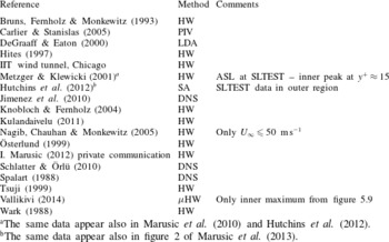
derived in § 2 from the momentum balance is continued across the entire boundary layer by fitting experimental data. To avoid a bias towards particular experiments, a comprehensive search of data from nearly every ZPG boundary layer experiment over a number of years was conducted. Of the experimental
 $\langle uu\rangle ^{+}$
profiles, only those have been retained for which the complete information on experimental conditions, probe characteristics, in particular the length of hot-wires, and all the corrections applied to the data was available. Hot-wire data not previously corrected for averaging were corrected with the scheme of Monkewitz, Duncan & Nagib (Reference Monkewitz, Duncan and Nagib2010). This screening resulted in 114 experimental profiles from 11 different sources being retained, as listed in table 3, together with the three sources of 14 DNS profiles.
Inspired by the leading-order linear dependence of the Taylor expansion of
 $\langle uu\rangle ^{+}$
on
 ${\it\epsilon}\equiv 1/U_{\infty }^{+}$
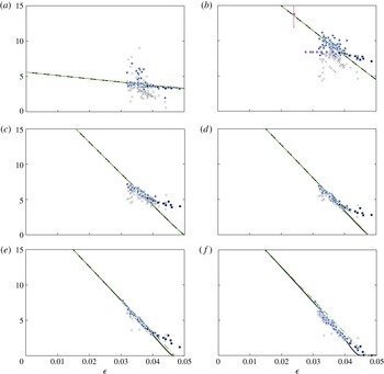
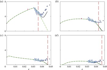
, the data have been interpolated to a number of fixed positions
 $y^{+}=\text{constant}$
and
 $Y\equiv y^{+}/\mathit{Re}_{{\it\delta}_{\ast }}=\text{constant}$
and plotted against
 ${\it\epsilon}$
in figures 8 and 9 respectively. It is evident from figure 8 that
 $\langle uu\rangle ^{+}$
remains close to a linear function of
 ${\it\epsilon}$
throughout the inner region, while its
 ${\it\epsilon}$
dependence at
 $Y=\text{constant}$
is rather complex. It should be noted here that
 $\mathit{Re}_{{\it\delta}_{\ast }}=10^{4}$
corresponds to
 ${\it\epsilon}=0.0366$
, and at
 ${\it\epsilon}=0.04$
the Reynolds number is already a marginal
 $\mathit{Re}_{{\it\delta}_{\ast }}=4160$
. Hence, it is expected that the data will start to deviate from our asymptotic high-Reynolds-number fits as
 ${\it\epsilon}$
approaches 0.04. The graphs are nevertheless extended to
 ${\it\epsilon}=0.05$
to show the continuous transition to low-Reynolds-number behaviour.
Data sources and acquisition methods: DNS, direct numerical simulation; HW, hot-wire anemometry; SA, sonic anemometer in the ASL (atmospheric surface layer); LDA, laser Doppler anemometer; PIV, particle image velocimetry. Additional HW and SA data in the outer logarithmic region up to
 $Y\approx 0.04$
can be found in figure 10(b) of Metzger, McKeon & Holmes (Reference Metzger, McKeon and Holmes2007). At
 $Y=0.015$
their data are approximately half an error bar above the data point in figure 9.

a The same data appear also in Marusic et al. (Reference Marusic, McKeon, Monkewitz, Nagib, Smits and Sreenivasan2010) and Hutchins et al. (Reference Hutchins, Chauhan, Marusic, Monty and Klewicki2012).
b The same data appear also in figure 2 of Marusic et al. (Reference Marusic, Monty, Hultmark and Smits2013).
Plot of
 $\langle uu\rangle ^{+}$
versus
 ${\it\epsilon}$
for different values of
 $y^{+}=\text{constant}$
: (a)
 $y^{+}=5$
; (b)
 $y^{+}=15$
; (c)
 $y^{+}=50$
; (d)
 $y^{+}=100$
; (e)
 $y^{+}=200$
; (f)
 $y^{+}=400$
. Data of table 3: (black) ▪, DNS data; (blue) ♦ , all other corrected data; (grey)
 $\times$
, uncorrected data; (purple) ▴ , inner maxima of Vallikivi (Reference Vallikivi2014); (pink) ●, inner peak of SLTEST data; (green) – ⋅ – ⋅ – , inner expansion (4.1); (black) ——, composite expansion (4.9).

Plot of
 $\langle uu\rangle ^{+}$
versus
 ${\it\epsilon}$
for different values of
 $Y=\text{constant}$
: (a)
 $Y=0.015$
; (b)
 $Y=0.1$
; (c)
 $Y=0.18$
; (d)
 $Y=0.2$
. Data of table 3: (black) ▪, DNS data; (blue) ♦ , all other corrected data; (grey)
 $\times$
, uncorrected data; (pink) ●, SLTEST; (green) - - -, outer expansion (4.7); (black) ——, composite expansion (4.9); (brown) vertical - - -,
 ${\it\epsilon}$
corresponding to
 $y^{+}=200$
.

Based on the data of figure 8, an inner expansion of
 $\langle uu\rangle ^{+}$
compatible with the Taylor expansion developed in § 2 has been constructed. It is given by
 $$\begin{eqnarray}\displaystyle \langle uu\rangle _{\mathit{inner}}^{+} & = & \displaystyle A(y^{+})-{\it\epsilon}\,B(y^{+}),\quad \text{with}\end{eqnarray}$$
 $$\begin{eqnarray}\displaystyle A(y^{+}) & = & \displaystyle A_{\infty }\tanh \left[\frac{t_{2,0}^{(uu)}(y^{+})^{2}+t_{4,0}^{(uu)}(y^{+})^{4}}{A_{\infty }}+{\it\alpha}_{1}(y^{+})^{5}\right],\end{eqnarray}$$
 $$\begin{eqnarray}\displaystyle B(y^{+}) & = & \displaystyle \left(B_{\infty }-{\it\beta}_{\infty }\right)\tanh \left[-\frac{t_{2,1}^{(uu)}(y^{+})^{2}+t_{4,1}^{(uu)}(y^{+})^{4}}{B_{\infty }-{\it\beta}_{\infty }}+{\it\beta}_{1}(y^{+})^{5}\right]+{\it\beta}_{\infty }\exp \left[\frac{{\it\beta}_{2}}{(y^{+})^{2}}\right],\nonumber\\ \displaystyle & & \displaystyle\end{eqnarray}$$
where the
 $t^{(uu)}$
are the coefficients of the Taylor expansion determined from the momentum balance in § 2 and given by (2.19) and (2.20), i.e.,
 $\{t_{2,0}^{(uu)},t_{2,1}^{(uu)},t_{4,0}^{(uu)},t_{4,1}^{(uu)}\}=\{0.26,-2.05,-0.0029,0.033\}$
. It is noted that the exponential in the expression for
 $B(y^{+})$
is exponentially small for both
 $y^{+}\rightarrow 0$
and
 $y^{+}=\mathit{O}({\it\epsilon}^{-1})$
so that it does not contribute to the Taylor expansion of
 $\langle uu\rangle _{inner}^{+}$
.
The parameters in (4.1) providing the best overall fit to the data of table 3 are
 $$\begin{eqnarray}\displaystyle \left.\begin{array}{@{}c@{}}\left\{A_{\infty };{\it\alpha}_{1}\right\}=\left\{22;1.5\times 10^{-5}\right\}\\ \left\{B_{\infty };{\it\beta}_{\infty };{\it\beta}_{1};{\it\beta}_{2}\right\}=\left\{470;130;1.5\times 10^{-5};-550\right\}\end{array}\!\right\}. & & \displaystyle\end{eqnarray}$$
Figure 8(a) for
 $y^{+}=5$
shows that the fit (4.1) has been constructed to match up to the Taylor expansion of the DNS data analysed in § 2. The full advantage of our approach can be appreciated in figure 8(b) for
 $y^{+}=15$
(see also figure 12), which shows the inner maxima of the present multisource data set, together with the linear fit (4.1) at
 $y^{+}=15$
, which is well approximated by
 $$\begin{eqnarray}\langle uu\rangle _{\mathit{peak}}^{+}(y^{+}\approx 15)\approx A_{\infty }-{\it\epsilon}\,(B_{\infty }-{\it\beta}_{\infty })=22-340\,{\it\epsilon}.\end{eqnarray}$$
This fit is seen to also nicely capture the peak value of the atmospheric SLTEST experiments (Metzger & Klewicki Reference Metzger and Klewicki2001), but does not agree with the
 $\mathit{Re}$
-independent maxima measured off figure 5.9 of Vallikivi (Reference Vallikivi2014). The latter NSTAP measurements are included to alert the reader to the existence of data that do not follow the linear dependence of
 $\langle uu\rangle _{\mathit{max}}^{+}$
on
 ${\it\epsilon}$
(see also appendix A). At this time we have no explanation for this difference, but find it rather unlikely that the Reynolds number dependence of
 $\langle uu\rangle _{\mathit{peak}}^{+}$
in the ZPG TBL should suddenly disappear for
 ${\it\epsilon}\lesssim 0.038$
.
For
 $y^{+}\rightarrow \infty$
,
 $\langle uu\rangle ^{+}$
finally reaches
 $$\begin{eqnarray}\langle uu\rangle _{\mathit{inner}}^{+}(y^{+}\rightarrow \infty )=A_{\infty }-{\it\epsilon}\,B_{\infty }=22-470\,{\it\epsilon},\end{eqnarray}$$
which corresponds to the level of
 $\langle uu\rangle ^{+}$
before its logarithmic decrease.
As seen from (4.3), we have chosen a relatively simple monotonically decreasing fit between the inner maximum (4.5) and the outer ‘plateau’ (4.6) because, given the increasing data uncertainty towards the wall and the scarcity of
 $\langle uu\rangle ^{+}$
profiles at large enough
 $\mathit{Re}_{{\it\delta}_{\ast }}$
above say 50 000, we do not find enough support for a minimum of
 $\langle uu\rangle ^{+}$
between the inner peak and the start of the outer logarithmic decay. This is, however, not to say that such a minimum can be positively excluded. If it existed, it could be easily fitted by increasing the coefficient of the exponential in the fit (4.3) for
 $B(y^{+})$
beyond
 ${\it\beta}_{\infty }$
and adding a
 $(1+\tanh )$
-like function to bring
 $\langle uu\rangle _{\mathit{inner}}^{+}$
back to the level given by (4.6).
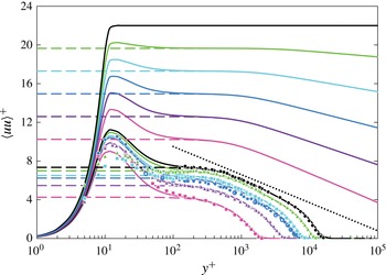
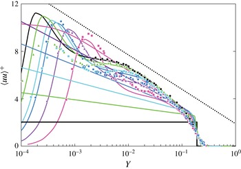
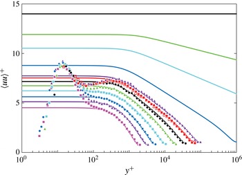
Selected profiles of
 $\langle uu\rangle ^{+}(y^{+})$
: - - - -, outer expansions (4.7); ——, composite expansions (4.9);
 $\cdots \cdots$
, logarithmic slope of
 $-1.26$
proposed by Marusic et al. (Reference Marusic, Monty, Hultmark and Smits2013). Data with fits: (pink) ▪, Bruns et al. (Reference Bruns, Fernholz and Monkewitz1993) with
 ${\it\epsilon}=0.0370$
, i.e.
 $\mathit{Re}_{{\it\delta}_{\ast }}=7.58\times 10^{3}$
; (purple) ▴, Kulandaivelu (Reference Kulandaivelu2011) with
 ${\it\epsilon}=0.0351$
, i.e.
 $\mathit{Re}_{{\it\delta}_{\ast }}=1.65\times 10^{4}$
; (blue) ●, I. Marusic, private communication with
 ${\it\epsilon}=0.0335$
, i.e.
 $\mathit{Re}_{{\it\delta}_{\ast }}=2.72\times 10^{4}$
; (dark blue) ○ , Knobloch & Fernholz (Reference Knobloch, Fernholz and Smits2004) with
 ${\it\epsilon}=0.0335$
, i.e.
 $\mathit{Re}_{{\it\delta}_{\ast }}=2.67\times 10^{4}$
; (light blue) ▪, IIT wind tunnel, Chicago, with
 ${\it\epsilon}=0.0329$
, i.e.
 $\mathit{Re}_{{\it\delta}_{\ast }}=3.28\times 10^{4}$
; (green) ▴, IIT wind tunnel, Chicago, with
 ${\it\epsilon}=0.0319$
, i.e.
 $\mathit{Re}_{{\it\delta}_{\ast }}=4.74\times 10^{4}$
; (black) ●, Kulandaivelu (Reference Kulandaivelu2011) with
 ${\it\epsilon}=0.0311$
, i.e.
 $\mathit{Re}_{{\it\delta}_{\ast }}=6.15\times 10^{4}$
. Only fits: (pink),
 ${\it\epsilon}=0.025$
, i.e.
 $\mathit{Re}_{{\it\delta}_{\ast }}=1.32\times 10^{6}$
; (purple),
 ${\it\epsilon}=0.02$
, i.e.
 $\mathit{Re}_{{\it\delta}_{\ast }}=6.14\times 10^{7}$
; (dark blue),
 ${\it\epsilon}=0.015$
, i.e.
 $\mathit{Re}_{{\it\delta}_{\ast }}=3.70\times 10^{10}$
; (light blue),
 ${\it\epsilon}=0.01$
, i.e.
 $\mathit{Re}_{{\it\delta}_{\ast }}=1.34\times 10^{16}$
; (green),
 ${\it\epsilon}=0.005$
, i.e.
 $\mathit{Re}_{{\it\delta}_{\ast }}=6.36\times 10^{32}$
; (black),
 ${\it\epsilon}=0$
, i.e.
 $\mathit{Re}_{{\it\delta}_{\ast }}=\infty$
.

In summary, our inner fit (4.1) produces peaks (4.5) that are always higher than the outer plateaus (4.6) until the two become equal at infinite Reynolds number (see figure 10). This view is broadly consistent with the distribution of turbulent energy production, which is strongly concentrated around
 $y^{+}\approx 10$
(see § 3). Hence, an outer maximum of
 $\langle uu\rangle ^{+}$
higher than the inner maximum at
 $y^{+}\approx 15$
could only arise from a significant depletion of
 $\langle vv\rangle ^{+}$
and
 $\langle ww\rangle ^{+}$
, for which we see no clear evidence. This is not to say that we exclude some redistribution between components. One could, for instance, argue that the slope of the fit in figure 8(c) for
 $y^{+}=50$
is slightly too high, i.e. that the asymptotic value of
 $\langle uu\rangle ^{+}({\it\epsilon}=0;y^{+}=50)$
should be below 22, but not lower than 15.
The outer expansion of
 $\langle uu\rangle ^{+}$
is constructed to fit the outer logarithmic decay with a Reynolds-number-dependent logarithmic slope, as shown in § 3. Matching up the logarithmic region to the plateau (4.6) at
 $y^{+}=\mathit{O}(1/{\it\epsilon})$
leads to the fit
 $$\begin{eqnarray}\displaystyle \langle uu\rangle _{\mathit{outer}}^{+}=\left\{A_{\infty }-{\it\epsilon}\,B_{\infty }-{\it\gamma}_{\infty }\,{\it\epsilon}\ln [1+({\it\gamma}_{1}\,{\it\epsilon}\,y^{+})^{2}]\hspace{-1.0pt}\right\}\frac{1}{2}\left\{1-\tanh \left[\frac{Y-Y_{d}}{{\it\gamma}_{2}\,{\it\epsilon}}\right]\hspace{-1.0pt}\right\}, & & \displaystyle\end{eqnarray}$$
with the fitting parameters
 $$\begin{eqnarray}\left\{{\it\gamma}_{\infty };{\it\gamma}_{1};{\it\gamma}_{2};Y_{d}\right\}=\left\{26;0.06;2;0.19\right\}.\end{eqnarray}$$
The first factor in (4.7) describes the logarithmic decay starting around
 $y^{+}=(0.06{\it\epsilon})^{-1}$
and the second factor represents the final decay to zero centred at
 $Y_{d}=0.19$
. This outer cutoff is meant to model the turbulent–non-turbulent interface (TNTI) even though we have placed it slightly outside the location
 $Y\approx 0.17$
, where it has been observed by Chauhan et al. (Reference Chauhan, Philip, DeSilva, Hutchins and Marusic2014). It should also be noted that the thickness of the TNTI has been made proportional to
 ${\it\epsilon}$
to reflect its observed steepening with Reynolds number (see, e.g., Corrsin, & Kistler Reference Corrsin and Kistler1955).
The composite expansion of the normal stress is now simply given by
 $$\begin{eqnarray}\langle uu\rangle _{\mathit{comp}}^{+}=\langle uu\rangle _{\mathit{inner}}^{+}+\langle uu\rangle _{\mathit{outer}}^{+}-\left(A_{\infty }-{\it\epsilon}\,B_{\infty }\right).\end{eqnarray}$$
The infinite-Reynolds-number limit of the outer expansion (4.7) requires some care as it depends on whether one holds
 $\bar{y}\equiv y^{+}/\mathit{Re}_{{\it\delta}_{\ast }}^{1/2}$
or
 $Y\equiv y^{+}/\mathit{Re}_{{\it\delta}_{\ast }}$
constant. The first step is to express
 $\mathit{Re}_{{\it\delta}_{\ast }}$
in terms of
 ${\it\epsilon}$
: transforming
 $U_{\infty }^{+}=\ln (\mathit{Re}_{{\it\delta}_{\ast }})/{\it\kappa}+C_{0}$
(
 ${\it\kappa}=0.384$
,
 $C_{0}=3.30$
) to
 $U_{\infty }^{+}\equiv {\it\epsilon}^{-1}=\ln (\widetilde{C}_{0}\mathit{Re}_{{\it\delta}_{\ast }})/{\it\kappa}$
yields
 $\mathit{Re}_{{\it\delta}_{\ast }}=(\widetilde{C}_{0})^{-1}\,\exp ({\it\kappa}/{\it\epsilon})$
, with
 $\widetilde{C}_{0}=3.55$
. Hence, the infinite-Reynolds-number limit of
 $\langle uu\rangle _{\mathit{outer}}^{+}$
is
 $$\begin{eqnarray}\langle uu\rangle _{\mathit{outer}}^{+}({\it\epsilon}\rightarrow 0;Y=\text{const.})=A_{\infty }-2\,{\it\kappa}\,{\it\gamma}_{\infty }\quad \text{for}~Y<Y_{d}\end{eqnarray}$$
and zero for
 $Y>Y_{d}$
, while
 $$\begin{eqnarray}\langle uu\rangle _{\mathit{outer}}^{+}({\it\epsilon}\rightarrow 0;\bar{y}=\text{const.})=A_{\infty }-{\it\kappa}\,{\it\gamma}_{\infty }.\end{eqnarray}$$
The quality of the fit (4.7) can be appreciated in figure 9, which also includes the SLTEST data (see table 3 for the data source). In this figure, the drop of
 $\langle uu\rangle ^{+}({\it\epsilon}=0)$
to zero between
 $Y=0.18$
and
 $Y=0.2$
reflects the crossing of the TNTI placed at
 $Y=0.19$
.
Returning to the more common representation of
 $\langle uu\rangle ^{+}$
at fixed Reynolds number versus the wall-normal coordinate, figures 10 and 11 demonstrate that our fits also do a good job on the profiles. As said before, if the fitting was optimized for individual profiles, the fitting parameters would vary considerably between profiles and even more so between profiles from different sources.


5. Conclusions and outlook
The present confrontation of experimental and DNS data with the Reynolds equation, and in particular its asymptotic expansion, should have clearly shown that it is not possible to draw solid conclusions from individual
 $\langle uu\rangle ^{+}$
profiles. The reasons are rather obvious.
High-quality DNS is still limited to moderate Reynolds numbers at which the TBL is relatively far from its asymptotic state in the outer and overlap regions. On the other hand, well-controlled laboratory experiments have reached
 $U_{\infty }^{+}$
of approximately 30, at which the asymptotic regions are relatively well separated. However, in our opinion measurement technology has not kept pace with the increase of experimental Reynolds numbers, and turbulence data near the wall are generally saddled with large systematic errors which can easily exceed 10 % and are notoriously difficult to correct since absolute calibration standards do not exist.
In the outer parts of the TBL, laboratory data on
 $\langle uu\rangle ^{+}$
are much less affected by systematic probe errors, but problems often arise from the limited development length for the largest turbulence eddies. If their turnover time is estimated as
 ${\it\delta}_{\ast }/u_{{\it\tau}}$
, all of the known laboratory wind tunnels allow a maximum of 10–20 turnovers (this estimate goes down considerably if
 ${\it\delta}_{\ast }$
is replaced by
 ${\it\delta}_{99}$
). As a consequence, both experimental and DNS turbulence in the outer part of the TBL must still retain some memory of how the turbulence was initiated in the different facilities, which shows up as substantial data scatter in the figures of § 4 (see, e.g., Chauhan, Monkewitz & Nagib (Reference Chauhan, Monkewitz and Nagib2009) and figures 5–7 of Marusic et al. (Reference Marusic, McKeon, Monkewitz, Nagib, Smits and Sreenivasan2010)). Specifically, we have found the differences between data from different high-quality experiments to be considerably larger throughout the TBL than the statistical error within each set. Therefore, extrapolation of
 $\langle uu\rangle ^{+}$
to infinite Reynolds number with data from any single facility would produce rather different results, and we strongly believe that further progress is only possible with data from an ensemble of different high-quality facilities. Consistent with this appreciation, the data in figures 8 and 9 of § 4 have not been identified.
The main findings of this study are in the following illustrated by two figures. The first result is that the normal stress
 $\langle uu\rangle$
scales with
 $u_{{\it\tau}}^{2}$
throughout the ZPG TBL, which means that its inner peak at
 $y^{+}\approx 15$
approaches a finite value in the limit of
 $\mathit{Re}_{{\it\delta}_{\ast }}\rightarrow \infty$
. The peak height is estimated at
 $\langle uu\rangle _{\mathit{peak}}^{+}\sim 22{-}340\,{\it\epsilon}$
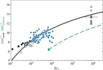
(4.5), which is seen in figure 12 to fit available data as well as a fit of the form
 $a+b\ln (\mathit{Re}_{{\it\delta}_{\ast }})$
, used extensively in the literature (see, e.g., Marusic et al.
Reference Marusic, McKeon, Monkewitz, Nagib, Smits and Sreenivasan2010) but incompatible with the inner scaling of
 $\langle uu\rangle$
demonstrated in § 2.
Inner maximum and outer plateau of
 $\langle uu\rangle ^{+}$
versus
 $\mathit{Re}_{{\it\tau}}$
: (black) ▪, (blue) ♦ , data of panel
 $y^{+}=15$
in figure 8; (black) ——, effective inner peak
 $22{-}346{\it\epsilon}$
of the fit (4.1); (grey)
 $\cdots \cdots$
, approximate inner peak given by (4.5); (green)
 $-~-~-$
, level of outer plateau
 $22{-}470{\it\epsilon}$
as function of Reynolds number; (green) ●, point where the plateau first appears in experimental profiles. It should be noted that
 $\mathit{Re}_{{\it\tau}}\approx 0.24\,\mathit{Re}_{{\it\delta}_{\ast }}$
since the boundary layer edge is located at
 $Y\approx 0.24$
. The ZPG TBL inner maxima reported in figure 1 of Marusic et al. (Reference Marusic, McKeon, Monkewitz, Nagib, Smits and Sreenivasan2010) for wind tunnel experiments (○) and for the SLTEST atmospheric TBL (
 $\triangle$
) are included for reference (see table 3 for the origin of the SLTEST data).

The second main finding is that the outer logarithmic slope of
 $\langle uu\rangle ^{+}$
is not constant, but decreases proportionally to
 ${\it\epsilon}$
. Furthermore, the scaling of the start of this logarithmic decay, or rather its intersection with the level of the outer plateau (or second maximum) at
 $y^{+}\approx (0.06~{\it\epsilon})^{-1}$
, has been derived from a simplified balance of turbulence production and dissipation in § 3.2. It is worth noting here that the outer fitting parameters and in particular the value of
 ${\it\gamma}_{1}=0.06$
in (4.8) have been obtained only with wind tunnel data. The atmospheric SLTEST data of Metzger et al. (Reference Metzger, McKeon and Holmes2007) suggest a value closer to 0.03, but we considered that the large total uncertainty of atmospheric measurements did not warrant an adaptation of the fitting parameters at this time. The geometry of the different domains of validity for the inner and outer asymptotic expansions of
 $U^{+}$
and
 $\langle uu\rangle ^{+}$
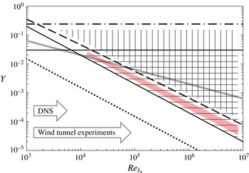
is summarized in figure 13. For
 $U^{+}$
the figure shows the overlap region bounded by
 $y^{+}=200$
and
 $Y=0.03$
where the average deviation from the mean velocity log law is below approximately 0.1 viscous units. It should be noted that this boundary of
 $Y=0.03$
corresponds very closely to the upper boundary of the log law in figure 3 of Marusic et al. (Reference Marusic, Monty, Hultmark and Smits2013), where
 $z\equiv y/{\it\delta}=0.1$
corresponds to
 $Y=0.024$
by virtue of
 ${\it\delta}/({\it\delta}_{\ast }\,U_{\infty }^{+})\approx 0.24$
.
Figure 13 clearly shows that at the Reynolds numbers of current ZPG TBL experiments the mean flow log law barely overlaps the logarithmic region of
 $\langle uu\rangle ^{+}$
. Actually, we see no good reason to look for a coincidence of the two log-law regions as in Marusic et al. (Reference Marusic, Monty, Hultmark and Smits2013) because their character is different. For the mean flow, the logarithmic region represents the overlap between the inner and outer asymptotic expansions of
 $U^{+}$
. Here, the logarithm is only possible because
 $U_{\mathit{inner}}$
scales with
 $u_{{\it\tau}}$
and
 $U_{\mathit{outer}}$
with
 $U_{\infty }$
. For the streamwise normal stress we have demonstrated that it scales with
 $u_{{\it\tau}}^{2}$
in both the inner and outer regions. This makes it impossible to connect inner and outer regions through a logarithmic overlap: if
 $\langle uu\rangle _{\mathit{outer}}^{+}\sim a-b\ln (Y)$
for
 $Y\rightarrow 0$
, the matching inner expansion would have to approach
 $\langle uu\rangle _{\mathit{inner}}^{+}\sim b\ln (\mathit{Re}_{{\it\delta}_{\ast }})+\mathit{O}(1)$
at large
 $y^{+}$
, in contradiction to its inner scaling. The actual overlap region between inner and outer expansions of
 $\langle uu\rangle ^{+}$
is the outer plateau, situated in the region
 $1\ll y^{+}\ll {\it\epsilon}^{-1}$
, where
 $\langle uu\rangle _{\mathit{overlap}}^{+}$
is given by (4.6).
The different regions of the asymptotic expansions of
 $U^{+}$
and
 $\langle uu\rangle ^{+}$
: horizontal hatching, overlap region of inner and outer expansions of
 $U^{+}$
bounded by
 $Y=0.03$
and
 $y^{+}=200$
, with the grey line marking the ‘centre’ of the overlap region
 $Y=2/\mathit{Re}_{{\it\delta}_{\ast }}^{1/2}$
; – ⋅ – ⋅ –, boundary layer edge at
 $Y\approx 0.24$
; - - - -, breakpoint
 $y^{+}=(0.06\,{\it\epsilon})^{-1}$
between outer plateau/maximum and logarithmic decay of
 $\langle uu\rangle ^{+}$
; vertical hatching, region where the outer logarithmic decay of
 $\langle uu\rangle ^{+}$
is clearly discernible; light red shading, overlap region of
 $\langle uu\rangle ^{+}$
(see text);
 $\cdots \cdots$
, location of inner peak at
 $y^{+}=15$
.

The overlap region of inner and outer expansions of
 $U^{+}$
, on the other hand, is
 $1\ll y^{+}\ll \mathit{Re}_{{\it\delta}_{\ast }}$
, and its ‘centre’ is located at the geometric mean
 $y^{+}/Re_{{\it\delta}_{\ast }}^{1/2}=\mathit{O}(1)$
. This apparent difference between the overlap regions of
 $U^{+}$
and
 $\langle uu\rangle ^{+}$
is puzzling, but we note that the mean flow log law represents the common part of the one-term inner and two-term outer expansions, while
 $\langle uu\rangle$
enters the asymptotic expansion of the momentum equation (2.3) at a higher order than
 $U$
(see § 2.2). Now it is well known that the extent of the overlap between inner and outer asymptotic expansions and the location of its ‘centre’ generally depend on the number of terms kept in each expansion. Therefore, if one could continue the inner and outer asymptotic expansions of
 $U^{+}$
to terms of the same order as the
 $x$
derivative of
 $\langle uu\rangle ^{+}$
in the momentum equation (we have only managed to do this for the Taylor expansions), the wall-normal extent of the
 $U^{+}$
overlap would probably shrink and its ‘centre’ might actually shift to the narrow overlap region of
 $\langle uu\rangle ^{+}$
, shaded red in figure 13 and bounded by
 $y^{+}=200$
and
 $y^{+}=(0.06\,{\it\epsilon})^{-1}$
. This is, however, just speculation on our part, and it is not clear at this point whether such a major analytical effort could be successful, as higher-order corrections of
 $U^{+}$
are too small to expect help from experimental data or ZPG TBL DNS.
Another open problem is how the asymptotic expansion of
 $\langle uu\rangle _{\mathit{inner}}^{+}$
in terms of powers of
 ${\it\epsilon}$
continues beyond the linear term considered in this paper. From the successful balancing of the Taylor-expanded momentum equation in § 2.2 and from the data in figure 8, it can be inferred that the
 ${\it\epsilon}^{2}$
terms in the asymptotic expansions of
 $\mathscr{X}$
(2.6a,b
and figure 3) and of
 $\langle uu\rangle _{\mathit{inner}}^{+}$
are small or possibly zero. It is, however, not clear at present how to obtain formal estimates for these
 ${\it\epsilon}^{2}$
terms.
Profiles of
 $\langle uu\rangle ^{+}(y^{+})$
in the ‘superpipe’ from Hultmark et al. (Reference Hultmark, Vallikivi, Bailey and Smits2012): ——, corresponding outer expansions (A 1). Data with fits: (pink) ▪,
 $\mathit{Re}_{{\it\tau}}=2.0\times 10^{3}$
; (purple) ▴,
 $\mathit{Re}_{{\it\tau}}=3.3\times 10^{3}$
; (blue) ●,
 $\mathit{Re}_{{\it\tau}}=5.4\times 10^{3}$
; (light blue) ▪,
 $\mathit{Re}_{{\it\tau}}=1.0\times 10^{4}$
; (green) ▴,
 $\mathit{Re}_{{\it\tau}}=2.0\times 10^{4}$
; (black) ●,
 $\mathit{Re}_{{\it\delta}_{\ast }}=3.8\times 10^{4}$
; (red) ▪,
 $\mathit{Re}_{{\it\tau}}=6.8\times 10^{4}$
(30
 ${\rm\mu}$
m wire); (red) ▫,
 $\mathit{Re}_{{\it\tau}}=6.8\times 10^{4}$
(60
 ${\rm\mu}$
m wire); (purple) ▴,
 $\mathit{Re}_{{\it\tau}}=9.8\times 10^{4}$
. Only fits: (blue),
 $\mathit{Re}_{{\it\tau}}=10^{6}$
; (light blue),
 $\mathit{Re}_{{\it\tau}}=10^{9}$
; (green),
 $\mathit{Re}_{{\it\tau}}=10^{15}$
; (black),
 $\mathit{Re}_{{\it\tau}}=\infty$
.

Finally, there is the issue of universality of the near-wall region in ‘canonical’ wall-bounded turbulent flows, including the ZPG TBL, channel and pipe flows. For the mean profile
 $U^{+}(y^{+})$
, this debate has focused on the value of the von Kármán constant (see, e.g., the clear exposition by Nagib & Chauhan Reference Nagib and Chauhan2008) and is still not finally settled. However, the differences between the values of
 $U_{\mathit{inner}}^{+}$
for the three canonical flows are minor compared with the difference between measured streamwise normal stresses in the ZPG TBL and in the pipe, for instance. To illustrate this point, we have fitted in appendix A the outer part of the NSTAP
 $\langle uu\rangle ^{+}$
profiles of Hultmark et al. (Reference Hultmark, Vallikivi, Bailey and Smits2012) with the function (A 1), which has essentially the same form as (4.7) with
 ${\it\epsilon}$
replaced by
 ${\it\mu}\equiv 1/\text{ln}(\mathit{Re}_{{\it\tau}})$
. As seen in figure 14, the scaling with
 ${\it\mu}^{-1}$
of the breakpoint between plateau or second maximum and the logarithmic decay, and the decrease of the logarithmic slope proportional to
 ${\it\mu}$
provide again excellent fits, but the fitting parameters, in particular the level of the plateau at infinite Reynolds number, are substantially different: while the common part of inner and outer expansions is
 $\langle uu\rangle _{\mathit{overlap}}^{+}\sim 22{-}470\,{\it\epsilon}$
in the ZPG TBL, it is
 $\langle uu\rangle _{\mathit{overlap}}^{+}\sim 14{-}72{\it\mu}$
in the pipe. This difference cannot be attributed only to the different definitions of
 ${\it\epsilon}\equiv 1/U_{\infty }^{+}$
and
 ${\it\mu}\equiv 1/\text{ln}(\mathit{Re}_{{\it\tau}})\sim 2.6\,{\it\epsilon}$
(this asymptotic relation is based on
 ${\it\delta}_{\ast }\approx 0.24{\it\delta}$
and
 $U_{\infty }^{+}={\it\kappa}^{-1}\ln (3.55\,\mathit{Re}_{{\it\delta}_{\ast }})$
). Therefore, the question is whether the presumed universality of canonical flows stops at the mean velocity profile. One may argue that a difference of
 $\langle uu\rangle$
is not surprising, since
 $\langle uu\rangle$
does not appear in the momentum equation for turbulent pipe flow, while in the ZPG TBL it is linked to
 $U$
through (2.3). However, this linkage is rather weak because of the
 $x$
derivative of
 $\langle uu\rangle$
, and the issue is likely to generate debate for some time to come.
Acknowledgements
We would like to thank all our colleagues who generously made their data available to us. Furthermore, we thank K. Chauhan, R. Duncan and R. Vinuesa for organizing and interpolating the data over a number of years while they were students at IIT.
Appendix A. Comparison with the ‘NSTAP’ data for
$\langle uu\rangle ^{+}$
in the ‘superpipe’

The outer part of the NSTAP pipe data of Hultmark et al. (Reference Hultmark, Vallikivi, Bailey and Smits2012) and Vallikivi (Reference Vallikivi2014) is fitted with the same functions as used in § 4 for the ZPG TBL, except close to the centreline. However, substantially different parameter values are required to fit the level of the outer plateau or maximum in particular. This is not only due to the difference between the outer coordinates
 $Y$
in the TBL and
 ${\it\eta}\equiv y/R$
in the pipe, and the difference between
 ${\it\epsilon}$
and the small parameter
 ${\it\mu}\equiv 1/\text{ln}(\mathit{Re}_{{\it\tau}})$
, with
 $\mathit{Re}_{{\it\tau}}\equiv Ru_{{\it\tau}}/{\it\nu}$
, but points to a genuine difference between the streamwise normal stresses in the ZPG TBL and in the pipe, where they do not appear in the momentum equation. Therefore, the arguments of § 2 pertaining to the inner region of
 $\langle uu\rangle$
are not applicable to the pipe, and the reader is referred to Hultmark et al. (Reference Hultmark, Vallikivi, Bailey and Smits2012) for arguments in favour of a constant inner peak height.
The main point of the comparison is to show that, despite the differences, the scaling
 $y_{\mathit{break}}^{+}=\mathit{O}(1/{\it\mu})$
for the intersection between backwards extrapolated logarithmic decay and the level of the outer peak as well as for a logarithmic slope
 $\propto {\it\mu}$
provides an excellent outer fit to the NSTAP data over the entire Reynolds number range. With a minor modification of the functional form of the fit (4.7) near the centreline to satisfy the symmetry condition, the outer part of
 $\langle uu\rangle ^{+}$
in the pipe is fitted by
 $$\begin{eqnarray}\displaystyle \langle uu\rangle _{outer}^{+} & = & \displaystyle A_{\infty }-{\it\mu}\,B_{\infty }-{\it\gamma}_{\infty }\,{\it\mu}\ln \left\{1+\left[{\it\gamma}_{1}\,{\it\mu}\,y^{+}\,(1+1.8\,{\it\eta}^{2}-1.28\,{\it\eta}^{4})\right]^{2}\right\},\nonumber\\ \displaystyle & & \displaystyle \text{with}~\left\{A_{\infty };~B_{\infty }\right\}=\left\{14;72\right\}~\text{and}~\left\{{\it\gamma}_{\infty };~{\it\gamma}_{1}\right\}=\left\{6.9;~0.021\right\}.\end{eqnarray}$$
The quality of this outer fit (A 1) is demonstrated in figure 14. It is interesting to note that, in the limit of infinite Reynolds number, these parameters yield at any fixed
 ${\it\eta}$
 $$\begin{eqnarray}\langle uu\rangle ^{+}({\it\eta}=\text{const.};{\it\mu}=0)=A_{\infty }-2\,{\it\gamma}_{\infty }=0.2,\end{eqnarray}$$
which is within a fitting accuracy of zero and may be compared with the limit (4.10) for the TBL. However, no speculation as to whether this limit should be zero or not can be offered at present.
Appendix B. The von Kármán integrated momentum equation and the evaluation of streamwise derivatives
The following derivations are improved and streamlined versions of the ones in Monkewitz et al. (Reference Monkewitz, Chauhan and Nagib2007), abbreviated here as MCN07, and serve to make the analytical part of this paper self-contained.
The von Kármán integral momentum equation is a mainstay of every textbook (see, e.g., Pope Reference Pope2000, § 5.2.1) but is often amputated without sufficient justification, as already remarked upon by Mellor (Reference Mellor1972). The pressure within the ZPG TBL is obtained from the wall-normal momentum equation, which is reduced to the terms that contribute to the orders retained in the asymptotic expansions of § 2.2 (note that for the next order in these asymptotic expansions, the term
 $-\partial \langle uv\rangle /\partial x$
would have to be included below):
 $$\begin{eqnarray}0=-\frac{1}{{\it\rho}}\,\frac{\partial P}{\partial y}-\frac{\partial \langle vv\rangle }{\partial y}.\end{eqnarray}$$
Introduction into the streamwise momentum equation leads to an expanded version of (5.56) of Pope (Reference Pope2000):
 $$\begin{eqnarray}U\frac{\partial U}{\partial x}+V\frac{\partial U}{\partial y}={\it\nu}\frac{\partial ^{2}U}{\partial y^{2}}-\frac{\partial \langle uv\rangle }{\partial y}-\frac{\partial }{\partial x}\left[\langle uu\rangle -\langle vv\rangle \right].\end{eqnarray}$$
As shown in the following, the streamwise gradient of the normal Reynolds stresses
 $\langle uu\rangle$
and
 $\langle vv\rangle$
has to be retained for high-Reynolds-number asymptotics beyond the leading terms.
Integrating (B 2) with respect to
 $y$
from the wall to the free stream and rearranging yields the von Kármán integrated momentum equation, with
 ${\it\theta}$
the momentum thickness, up to the terms required for the near-wall analysis of § 2.2:
 $$\begin{eqnarray}\frac{1}{(U_{\infty }^{+})^{2}}=\frac{\text{d}{\it\theta}}{\text{d}x}-\frac{1}{U_{\infty }^{2}}\frac{\text{d}}{\text{d}x}\int _{0}^{\infty }\!\left[\langle uu\rangle -\langle vv\rangle \right]\,\text{d}y.\end{eqnarray}$$
It should be noted that the sign of the normal stress difference in (4) of MCN07 is wrong, but only impacts their § V. To proceed, we make the following assumptions.
-
(i) The mean velocity in the ZPG TBL is fully described by the classical inner and outer layers, asymptotically matched in an overlap layer. In these two layers, the wall-normal coordinate
$y$
is scaled as
$y^{+}=yu_{{\it\tau}}/{\it\nu}$
and
$Y=y/({\it\delta}_{\ast }U_{\infty }^{+})$
respectively. -
(ii) The mean streamwise velocity
$U^{+}=U/u_{{\it\tau}}$
in the overlap layer is given asymptotically by the classical logarithmic law
$L^{+}={\it\kappa}^{-1}\ln y^{+}+B$
. -
(iii) The inequality
$\int _{0}^{\infty }\langle uu\rangle \,\text{d}y\geqslant \int _{0}^{\infty }\langle vv\rangle \,\text{d}y$
, experimentally verified at finite Reynolds numbers, remains valid in the limit of infinite Reynolds number.


Next, the momentum and displacement thicknesses need to be expressed in terms of the mean velocity profile. Using assumptions (i) and (ii), the complete mean velocity profile is given by the composite expansion (for the concept of composite expansions, see, e.g., Kevorkian & Cole Reference Kevorkian and Cole1985)
 $$\begin{eqnarray}U_{\mathit{comp}}^{+}=U_{\mathit{\,i}}^{+}(y^{+})-L^{+}(y^{+})+U_{\infty }^{+}-W^{+}(Y),\end{eqnarray}$$
where the logarithmic law
 $L^{+}={\it\kappa}^{-1}\ln y^{+}+B$
represents the common part of the inner and outer profiles
 $U_{\mathit{\,i}}^{+}(y^{+})$
and
 $U_{\infty }^{+}-W^{+}(Y)$
respectively. The matching of inner and outer profiles in the overlap region, where
 $\widetilde{y}=y^{+}(\mathit{Re}_{{\it\delta}_{\ast }})^{-1/2}=Y(\mathit{Re}_{{\it\delta}_{\ast }})^{+1/2}$
is of order
 $\mathit{O}(1)$
, leads to
 $$\begin{eqnarray}\displaystyle W^{+}\left(Y\rightarrow 0\right)\sim -\frac{1}{{\it\kappa}}\ln Y-B+C_{0}\quad \text{and}\quad U_{\infty }^{+}\sim \frac{1}{{\it\kappa}}\ln (\mathit{Re}_{{\it\delta}_{\ast }})+C_{0}. & & \displaystyle\end{eqnarray}$$
A continuation of the asymptotic expansion of
 $U_{\infty }^{+}$
beyond
 $C_{0}$
in terms of negative powers of
 $\ln (\mathit{Re}_{{\it\delta}_{\ast }})$
is left open, as it only impacts higher-order terms not considered in this paper. With (B 4) the displacement and momentum thicknesses are
 $$\begin{eqnarray}\displaystyle {\it\delta}_{\ast } & \equiv & \displaystyle \int _{0}^{\infty }\left[1-\frac{U_{\mathit{comp}}^{+}}{U_{\infty }^{+}}\right]\text{d}y={\it\delta}_{\ast }\,\int _{0}^{\infty }W^{+}\,\text{d}Y-\,\frac{{\it\delta}_{\ast }}{\mathit{Re}_{{\it\delta}_{\ast }}}\int _{0}^{\infty }\left[U_{\mathit{\,i}}^{+}-L^{+}\right]\,\text{d}y^{+},\end{eqnarray}$$
 $$\begin{eqnarray}\displaystyle {\it\theta} & \equiv & \displaystyle \int _{0}^{\infty }\frac{U_{\mathit{comp}}^{+}}{U_{\infty }^{+}}\,\left[1-\frac{U_{\mathit{comp}}^{+}}{U_{\infty }^{+}}\right]\,\text{d}y={\it\delta}_{\ast }\left\{\int _{0}^{\infty }W^{+}\,\text{d}Y-\frac{1}{U_{\infty }^{+}}\int _{0}^{\infty }\left(W^{+}\right)^{2}\,\text{d}Y\right\}\nonumber\\ \displaystyle & & \displaystyle +\,\frac{{\it\delta}_{\ast }}{\mathit{Re}_{{\it\delta}_{\ast }}}\left\{\int _{0}^{\infty }\left[U_{\mathit{i}}^{+}-L^{+}\right]\,\text{d}y^{+}-\frac{1}{U_{\infty }^{+}}\int _{0}^{\infty }\left[(U_{\mathit{i}}^{+})^{2}-(L^{+})^{2}\right]\,\text{d}y^{+}\right\},\end{eqnarray}$$
leading to an integral constraint on
 $W^{+}$
and an expression for the shape factor
 $H$
(see also MCN07):
 $$\begin{eqnarray}\displaystyle & \displaystyle \int _{0}^{\infty }W^{+}\,\text{d}Y=1+\mathscr{B}\mathit{O}\left(\mathit{Re}_{{\it\delta}_{\ast }}\right)^{-1}\quad \text{and} & \displaystyle\end{eqnarray}$$
 $$\begin{eqnarray}\displaystyle & \displaystyle \frac{{\it\theta}}{{\it\delta}_{\ast }}\equiv H^{-1}=1-\frac{1}{U_{\infty }^{+}}\,\int _{0}^{\infty }\left(W^{+}\right)^{2}\,\text{d}Y+\mathscr{B}\mathit{O}\left(\mathit{Re}_{{\it\delta}_{\ast }}\right)^{-1}. & \displaystyle\end{eqnarray}$$
Here,
 $\mathscr{B}\mathit{O}$
designates ‘block order’, a concept that has been introduced by Crighton & Leppington (Reference Crighton and Leppington1973) and consists of lumping all of the terms
 ${\it\epsilon}^{n}\times (-\ln {\it\epsilon})^{m}$
with the same power
 $n$
into one block, irrespective of
 $m$
. The block order is related to the standard order relation
 $\mathit{O}$
by
 $\mathscr{B}\mathit{O}({\it\epsilon}^{n})\equiv \mathit{O}[{\it\epsilon}^{n}(-\ln {\it\epsilon})^{M}]$
, with
 $M$
the largest power of
 $(-\ln {\it\epsilon})$
in the block.
To determine the
 $x$
derivatives of
 ${\it\delta}_{\ast }$
and
 ${\it\theta}$
from the integrated momentum equation (B 3), one has to make an assumption on the scaling of the normal stresses, taken to be identical for all components (different scalings for each component are possible, but do not fundamentally change the following arguments). Three possibilities are considered for the scaling of normal stresses in all the regions of the boundary layer:
 $$\begin{eqnarray}\langle \cdot \,\cdot \rangle \equiv u_{{\it\tau}}^{2-m}U_{\infty }^{m}\langle \cdot \,\cdot \rangle ^{\oplus },\end{eqnarray}$$
where
 $m=0,1,2$
corresponds to inner, mixed and outer scaling respectively. With (B 10), the second term on the right-hand side of (B 3) becomes
 $$\begin{eqnarray}-\frac{\text{d}}{\text{d}x}\left\{{\it\delta}_{\ast }(U_{\infty }^{+})^{m-1}\int _{0}^{\infty }\!\left[\langle uu\rangle ^{\oplus }-\langle vv\rangle ^{\oplus }\right]\,\text{d}Y\right\},\end{eqnarray}$$
where the integral over the inner part of the normal stress difference contributes only at order
 $\mathscr{B}\mathit{O}(\mathit{Re}_{{\it\delta}_{\ast }}^{-1})$
, as in (B 8) and (B 7). Finally, both
 $W^{+}$
and
 $[\langle uu\rangle ^{\oplus }-\langle vv\rangle ^{\oplus }]$
must be expected to have asymptotic expansions in terms of inverse powers of
 $U_{\infty }^{+}$
, which translates to the following expansions for the integrals:
 $$\begin{eqnarray}\displaystyle & \displaystyle \int _{0}^{\infty }\left(W^{+}\right)^{2}\,\text{d}Y\sim I_{\mathit{ww}}^{(0)}+\,\mathit{O}\left(U_{\infty }^{+}\right)^{-1}\quad \text{and} & \displaystyle \nonumber\\ \displaystyle & \displaystyle \int _{0}^{\infty }\left[\langle uu\rangle ^{\oplus }-\langle vv\rangle ^{\oplus }\right]\,\text{d}Y\sim I_{\mathit{nsd}}^{(0)}+\frac{1}{U_{\infty }^{+}}\,I_{\mathit{nsd}}^{(1)}+\mathit{O}\left(U_{\infty }^{+}\right)^{-2}. & \displaystyle\end{eqnarray}$$
Introduction of (B 9), (B 11) and the expansions (B 12a,b ) into the integrated momentum equation (B 3) finally yields
 $$\begin{eqnarray}\displaystyle \displaystyle \frac{1}{(U_{\infty }^{+})^{2}} & = & \displaystyle \displaystyle \frac{\text{d}{\it\delta}_{\ast }}{\text{d}x}\,\left\{1-\frac{I_{\mathit{ww}}^{(0)}}{U_{\infty }^{+}}+\mathit{O}\left(U_{\infty }^{+}\right)^{-2}\right\}\nonumber\\ \displaystyle & & \displaystyle \quad -\left\{\frac{\text{d}{\it\delta}_{\ast }}{\text{d}x}\left(U_{\infty }^{+}\right)^{m-1}+(m-1){\it\delta}_{\ast }\left(U_{\infty }^{+}\right)^{m-2}\frac{\text{d}U_{\infty }^{+}}{\text{d}x}\right\}\nonumber\\ \displaystyle & & \displaystyle \displaystyle \quad \times \left\{I_{\mathit{nsd}}^{(0)}+\frac{1}{U_{\infty }^{+}}\,I_{\mathit{nsd}}^{(1)}+\,\mathit{O}\left(U_{\infty }^{+}\right)^{-2}\right\}\nonumber\\ \displaystyle & & \displaystyle \displaystyle \quad +\,{\it\delta}_{\ast }\left(U_{\infty }^{+}\right)^{m-3}\frac{\text{d}U_{\infty }^{+}}{\text{d}x}\left\{I_{\mathit{nsd}}^{(1)}+\mathit{O}\left(U_{\infty }^{+}\right)^{-1}\right\}.\end{eqnarray}$$
With (B 5a,b
), the
 $x$
derivative of
 $U_{\infty }^{+}$
is related to the derivative of
 ${\it\delta}_{\ast }$
by
 $$\begin{eqnarray}\frac{\text{d}U_{\infty }^{+}}{\text{d}x}=\frac{1}{{\it\kappa}\,{\it\delta}_{\ast }}\frac{\text{d}{\it\delta}_{\ast }}{\text{d}x}\left\{1+\mathit{O}\left(U_{\infty }^{+}\right)^{-2}\right\},\end{eqnarray}$$
so that the
 $x$
derivative of
 ${\it\delta}_{\ast }$
is finally obtained from (B 13) for the three choices of
 $m$
:
 $$\begin{eqnarray}\displaystyle & \displaystyle m=0\text{ (inner scaling),}\quad \frac{\text{d}{\it\delta}_{\ast }}{\text{d}x}\sim \frac{1}{(U_{\infty }^{+})^{2}}\left\{1+\frac{I_{\mathit{ww}}^{(0)}+I_{\mathit{nsd}}^{(0)}}{U_{\infty }^{+}}+\mathit{O}\left(U_{\infty }^{+}\right)^{-2}\right\}; & \displaystyle\end{eqnarray}$$
 $$\begin{eqnarray}\displaystyle & \displaystyle m=1\text{ (mixed scaling),}\quad \frac{\text{d}{\it\delta}_{\ast }}{\text{d}x}\sim \frac{1}{(1-I_{\mathit{nsd}}^{(0)})\,(U_{\infty }^{+})^{2}}\left\{1+\mathit{O}\left(U_{\infty }^{+}\right)^{-1}\right\}; & \displaystyle\end{eqnarray}$$
 $$\begin{eqnarray}\displaystyle & \displaystyle m=2\text{ (outer scaling),}\quad \frac{\text{d}{\it\delta}_{\ast }}{\text{d}x}\sim \frac{-1}{I_{\mathit{nsd}}^{(0)}\,(U_{\infty }^{+})^{3}}\left\{1+\mathit{O}\left(U_{\infty }^{+}\right)^{-1}\right\}. & \displaystyle\end{eqnarray}$$
The result (B 17) clearly rules out outer scaling for the normal stresses if the relatively weak hypotheses at the beginning of this section are accepted (note that the argument in MCN07 against outer scaling must be ignored due to the sign error mentioned earlier). As for mixed scaling of
 $\langle uu\rangle$
, it cannot be excluded on the basis of the von Kármán integrated momentum equation (B 3). However, it is shown in § 2.2 that the momentum equation (B 2) can only be satisfied if the inner parts of
 $\langle uu\rangle$
and
 $\langle vv\rangle$
are scaled with
 $u_{{\it\tau}}^{2}$
. Besides, the reader is left to ponder the awkward consequences of scaling the fluctuating velocity
 $u^{\prime }$
with
 $(u_{{\it\tau}}U_{\infty })^{1/2}$
. The inner scaling of the outer parts of
 $\langle uu\rangle$
and
 $\langle vv\rangle$
then follows from the straightforward matching arguments of § 4.
Finally, a relation between the distance
 $x$
from the virtual origin of the ZPG TBL and
 ${\it\delta}_{\ast }$
is easily obtained by using (B 5a,b
) for
 $U_{\infty }^{+}(\mathit{Re}_{{\it\delta}_{\ast }})$
and integrating the result (B 15) for
 $m=0$
, which is identified in § 2.2 as the only possible choice, leading to
 $$\begin{eqnarray}\frac{x}{{\it\delta}_{\ast }}=(U_{\infty }^{+})^{2}\left\{1+\frac{I_{\mathit{ww}}^{(0)}+I_{\mathit{nsd}}^{(0)}+2{\it\kappa}^{-1}}{U_{\infty }^{+}}+\mathit{O}\left(U_{\infty }^{+}\right)^{-2}\right\}.\end{eqnarray}$$
A relation for
 $x({\it\theta})$
, analogous to (B 18), has already been given in MCN07 as (24). However, it did not include the integral
 $I_{\mathit{nsd}}$
and the inversion
 ${\it\theta}(x)$
(25) was too messy to be useful. To obtain
 ${\it\delta}_{\ast }$
as a function of
 $x$
, (B 18) is best inverted numerically.