LAW v. POLITICS

Judicial decision making has unique characteristics that distinguish it from decision making in legislative settings. A judge makes policy by resolving legal disputes, that is, by deciding cases that present themselves as bundles of facts. Murphy (1964) notes that the need to make policy through individual cases is one of the more important technical checks on judges. Even the most ideological and policy-oriented appellate judge must make policy by telling lower court judges what facts to consider and what those facts mean for case outcomes. Even a dictatorial judge cannot just list all desired dispositions for every possible case that might arise. He or she must provide some framework or guideline for lower courts and future judges to follow, a legal doctrine or rule for sorting out winners and losers. Thus, judge-created rules are the heart of judicial policy.

This holds whether his or her preferences for who wins are ideological or derived from normative principles or a legal philosophy. To be sure, the application of legal rules is the core of law and legal theory, but thinking of judges as political creatures does not obviate the need to think about cases and rules. From either a purely political or purely legal perspective, rules, cases, and case facts are quite significant concepts—yet political models of judicial policy making, formal and otherwise, often pay little attention to them.

This is, perhaps, understandable. The founding debate of judicial politics—whether judges make law or find law—yielded an uneasy relationship with legal doctrine. In rejecting law as an exogenous constraint on choice, any role for legal rules or doctrine became suspect. In stressing ideological goals, the structure and substance of judicial preferences were set aside. In emphasizing the freedom of Supreme Court justices to pursue policy goals, the instruments by which they might do so were neglected. Perhaps for these reasons, even some legal scholars who agree that judging can be political argue that much political science trivializes law and the legal enterprise (e.g., Friedman 2006; Tiller and Cross 2006).

There are conflicts within political science as well. The Attitudinal Model (Segal and Spaeth 2002) focuses on the dichotomous votes of Supreme Court justices to affirm or reverse lower court decisions, arguing that justices cast such final votes solely and sincerely on the basis of personal ideology. Others study how justices interact in their pursuit of legal policy goals (e.g., Epstein and Knight 1998; Maltzman, Spriggs, and Wahlbeck 2000). But, what exactly is the content of the “legal policy” that is the focus of this interaction? How does legal policy as established in judicial opinions relate to case votes? Can we reconcile the primacy of sincere final votes over case dispositions with the (possibly strategic) policy choices justices make in writing opinions? Indeed, the nature of judicial preferences is a question theoretically prior to that of how preferences interact.

Formal models of judicial policy making often treat the objects of choice as points in a policy space, but this approach raises similar questions. What is a “case” in the standard spatial policy model? Is a policy point the outcome within a specific case? If so, what makes one case different from any other? How does a court's (mostly) passive reliance on cases to make policy constrain it? If judges make policy by deciding specific cases and creating and applying general legal rules, these concepts should at least be compatible with our modeling constructs—but how does a policy point capture how rules work?¹

Another issue is that the usage of the standard policy-space model often requires harsh simplifications. In a unidimensional setting, the median voter's ideal point represents a majoritarian policy, but in a multidimensional setting, there is usually no median ideal point, and hence no meaningful majoritarian policy point (let alone a stable one). This issue is usually avoided either by assuming collegial courts are unitary actors or by assuming unidimensionality. That is, instead of adapting formal theory to the substance of judicial politics, the set of choices or of players is arbitrarily cut to fit the needs of the abstract theory. I show that this Procrustean choice may be unnecessary.

The “case-space model” resolves many of these difficulties. While still invoking assumptions about choice, these are tailored substantively to the institutional features of judicial policy making. This model thus provides a structure for thinking about cases, facts, judgements, opinions, and legal rules, without rejecting a role for judicial preferences.

This model has its origins in Kornhauser (1992a,b), which specified the idea of a rule as a function that establishes equivalence classes of cases to be decided similarly. Cameron (1993) suggested a geometric version of this approach, with a spatial representation of cases and rules, but in this early version of the case-space, courts were explicitly assumed to be unitary actors. Grofman (1993) briefly considered unstructured rules from a collegial perspective. Cameron, Segal, and Songer (2000) used a unidimensional, unitary-actor case-space to study auditing in the judicial hierarchy. Lax (2003) analyzed a collegial, but still unidimensional, case-space model to explore the impact of the Supreme Court's institutional rules on compliance in the lower courts. Kastellec (2007) extended this model to explore whistle-blowing in the lower courts. The present paper studies a collegial court making policy in a multidimensional case space.²

CASES AND RULES

I first define the basics of the case-space model, cases and rules, and then define an important type of rule, a proper rule.

Cases

Judges resolve legal disputes; that is, they decide cases that present themselves as bundles of facts.³

Although on the surface a case space looks similar to a standard policy space, they differ in the assumptions made about the structure of choice. In a policy space, one makes policy by choosing a point. In contrast, in a case space, each point represents not a general policy, but a specific potential case. These case points are exogenously fixed, and when given a case to decide, a court chooses a disposition for it. Judicial policy making is then the mapping of fixed points to dispositions. In other words, the judicial choice is not “Which point shall I pick?”; rather it is “Which disposition shall I choose for this given point?” Indeed, cases are the fundamental units of judicial policy making—and a case-space model is specifically designed to capture the importance of these units.

Formally, a case is modeled as a point in a multidimensional case space, capturing its location (between 0 and 1) on each factual dimension:

Definition. A case is a point x in the unit m-hypercube, C^m, denoted by the vector (x₁, …, x_m), where

is the location of case xⁱ on dimension s≤m.

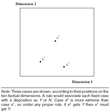
The factual dimensions capture whatever facts might be considered relevant to the judges. Figure 1 shows a two-dimensional case space and three sample case points.

Comparing Cases

Rules

When appellate courts address judicial policy more generally, they typically do so in opinions that establish (new or modified) legal rules for deciding current and future cases. Rules are thus the derivative unit of judicial policy making.

A judge will prefer one disposition or the other in each case, and so each case can be mapped to a disposition Y or N in the outcome space. Kornhauser (1992a) calls the list of such preferred dispositions an extended rule. This generic form of rule simply sorts cases into two equivalence classes, one getting Y and the other getting N. An extended rule C can be formally defined as a set, the set of cases that get decided as Y:

Definition. An extended rule is a closed set C such that the decision in case xⁱ is Y if and only if xⁱ∈C.

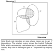
See Figure 2 for examples of extended rules. Note that an extended rule, as defined by Kornhauser, need have no special substance or structure. (Grofman [1993] similarly treats rules as amorphous sets of cases.) The set of Y outcomes need not be meaningfully shaped or even contiguous. In particular, extended rules make no use of the spatial setting. They need not be even minimally rational in how they allocate cases to dispositions. (The equivalent for a standard policy space might be non-single-peaked preferences or, more generally, dimensions which do not order points in a meaningful way.) Legal rules, on the other hand, are usually highly structured. I next add additional structure to case dimensions and then to sets of case dispositions.

Three Generic Rules and the Implicit Collegial Rule

Ordering Cases

Code each dimension such that the “mildest” case takes a value of 0 on all dimensions and the most “extreme” case takes a value of 1 on all dimensions (similar to the ordering of policy points in the standard policy space from least to most). Let more extreme values be those more conducive to a N outcome. For example, in equal protection cases (where the question is the constitutionality of a state's classification scheme based on race, gender, etc.), the dimensions might include (1) how “suspect” the class invoked is (coded directly), (2) how compelling the state interest is (coded inversely, so that a more compelling interest is more conducive to a Y), and (3) how necessary the classification is (again coded inversely). Or, these dimensions could be broken down further.

A case is more extreme on a particular dimension if it takes a higher value on that dimension. It is said to be more extreme than another case overall if it is more extreme on at least one dimension and not less extreme on any other. Thus, in Figure 1, case x¹ is less extreme than case x², but x³ is neither more nor less extreme overall than either x¹ or x² (of course, x³ is more extreme on dimension 1 and less extreme on dimension 2). Formally,

Definition. Case xⁱ is weakly more extreme than case x^w, denoted xⁱ[sce ]x^w, if for all s,

. It is strictly more extreme, xⁱ[sc ]x^w, if there exists t such that

.

This ordering of cases leads naturally to an intuitive type of rule.

Proper Rules

Assume a judge is (weakly) more inclined to vote N as the score on any one dimension increases. Call a rule with this monotonicity property a proper rule. Formally, a proper rule requires that, if a case xⁱ gets Y, then any case less extreme than xⁱ also gets Y (and that, if xⁱ gets N, then any case more extreme than xⁱ must also get N):

Definition. A rule C is a proper rule if and only if, for all xⁱ∈C and all x^w[pre ]xⁱ, x^w[pre ]xⁱ⇒x^w∈C.

Under this definition, a judge must not have “perverse” preferences. For example, if one dimension is the degree of probable cause in a search-and-seizure case, a judge does not want to strike searches simply because there is “more” probable cause. Or, more simply, driving slower should not be more likely to yield a “speeding” verdict than going faster. A judge may still think any or all dimensions irrelevant.

Although all proper rules are extended rules, not all extended rules are proper rules. In Figure 1, a proper rule would allow both x¹ and x² to get Y or both to get N or only x¹ to get Y, but a rule under which x² gets Y and x¹ gets N would not be a proper rule. A proper rule would allow either disposition for x³, no matter what is decided for the other two cases, since x³ is neither more nor less extreme overall. (An extended rule meanwhile would allow any combination of dispositions.)

If we focus on the boundary dividing Y cases from N cases, we can use an alternate and perhaps more intuitive formulation of a proper rule. A proper rule sets a limit, a limit representing how extreme a case can be before getting N (with all cases less extreme getting Y). Consider the speed limit, a simple proper rule in one dimension, with lower speeds permissible and any higher speed a violation. A more complicated speeding proper rule might set different limits for different traffic conditions or locations (55 under normal conditions, 30 in a school zone, 20 when it is snowing, etc.), again with any speed beneath the appropriate limit acceptable and any speed above subject to sanction. A proper rule thus has the sort of structure we tend to think of as associated with a legal rule (as compared to the unstructured extended rule).

To be a proper rule, the limit established must have certain features: Proposition 1. proper rule function Rule C is a proper rule if and only if there exists a function r(x₁, …, x_m−1) with two properties:

1. r(x₁, x₂, …, x_m−1) is weakly decreasing in all x_s<m; and
2. xⁱ∈C if and only if
   .

This function sets the limit for a Y, defined on one dimension (dimension m) with respect to the case's location on the other (m−1) dimensions. The boundary of a proper rule never has positive slope. (Of course, if the boundary always has positive slope, we could just flip axes so that the rule would be proper for the new configuration.) We can represent judge j's proper rule either by the boundary function r_j or by the set C itself (though only the former usage makes it clear that the rule is indeed a proper rule).

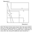
Even given this structural restriction, proper rules can still capture a wide variety of substantive rules, as in Figure 3, showing seven proper rules in a two-dimensional case space. (In comparison, none of the rules in Figure 2 are proper rules.) Any case above/to the right of the rule gets N and any case below/to the left of the rule gets Y. Judge G has the simplest rule; she never wants Y no matter what the case facts are. Judge A prefers a simple disjunctive rule (with the logical form Y[harr ]P∨Q)—a case must fall below a fixed threshold on dimension 1 or below a fixed threshold on dimension 2 to get Y. Judge B sees dimension 1 as irrelevant and wants a fixed (lower) threshold for dimension 2 (this rule takes the form Y[harr ]P). Judge C prefers a simple conjunctive rule (both thresholds must be met, yielding the logical form Y[harr ]P∧Q).⁴

Proper Rules

In one dimension, a proper rule is just a constant, a cut-point dividing Ys and Ns—and may seem similar to an ideal point in a standard policy space. In a multidimensional case space, however, a proper rule can no longer be just a point itself, as it generally takes more than a point to partition cases into Ys and Ns. The set of cases to be captured by a proper rule will potentially have as many dimensions as the space itself, and the limit must be defined across all but one of these. To divide points in a two-dimensional case space, we would need a (one-dimensional) plane curve, such as a line. In a three-dimensional case space, a proper rule must be a (two-dimensional) surface, such as a plane or part of a sphere. (Formally, a proper rule must be a co-dimension-one hypersurface.)⁶

Ordering Proper Rules

In standard policy spaces, we often label one direction liberal and the other conservative, and we call one policy more extreme than another. We can discuss proper rules in the same way. A rule might be more “conservative” the more cases it would decide as Y (or more “liberal,” depending on the issue area). If a given proper rule yields at least all the same Y outcomes as another rule, and includes still additional Y outcomes, we can say the former is a more extreme rule:

Definition. Proper rule C_j is more extreme than proper rule C_z if and only if C_z⊂C_j.

We can also state this condition in terms of the “limit” definition of a proper rule: Corollary 1. corollary 1 proper rule extreme Proper rule C_j is (weakly) more extreme than proper rule C_z if and only if r_j(x₁, x₂, …, x_m−1)≥r_z(x₁, x₂, …, x_m−1) for all x₁, x₂, …, x_m−1.

In Figure 3, rule A is more extreme than rule B, B is more extreme than C, and C is more extreme than E. Similarly, rule A is more extreme than rule D, and D is more extreme than E. (These are not exhaustive lists.) One difficulty in comparing rules is that a rule might be more liberal in some areas of the case space and less liberal in others. Comparing rules C and D, for example, rule D includes cases near the upper left as Y that rule C does not, whereas C includes cases toward the right of and excluded by D. (One could still, perhaps, compare the percentage of possible cases decided as Y under different rules to assess overall liberalism or conservatism.)

I next consider whether preferences over rules can be aggregated in a meaningful way.

A THEORY FOR AGGREGATING RULES

Assume there are k judges (k odd) and that judge j has extended rule C_j. Let this profile of rules be denoted r. The first key result is that there always exists a collegial rule—the Implicit Collegial Rule, or ICR—capturing those cases that get Y by majority vote: Proposition 2. ICR exists For any k rules (C₁, …, C_k), there exists an extended rule

(the Implicit Collegial Rule), such that

if and only if

.}

The ICR is the (closed) set of cases where a majority of rules overlap. A case is in this set if it is in at least

of the individual sets, and so applying the ICR has the same effect as the collegial court directly hearing a case and voting by majority rule. This set, however, is simply an extended rule, and so it need have no special structure. Figure 2 shows the set of cases that compose the ICR for a given set of individual extended rules.

Given the substantive primacy of proper rules, suppose that all k individual rules are proper rules. Then, we have the following key result: Proposition 3. proper ICR If all rules C₁, …C_k∈r are proper rules, then the Implicit Collegial Rule

is a proper rule.

That is, not only will there always an exist a collegial rule that has the same effect as the majoritarian aggregation of the judges' preferred proper rules, but this collegial rule will also be a proper rule itself—the aggregation of proper rules is a proper rule. Thus, collegiality will not induce perversity of group preference. If the individual preferences relate to the factual dimensions in a nonperverse way, so will the group preference.

The next step is to show what this rule is and how it relates to the individual proper rules. The following result defines the Implicit Median Rule (IMR) for any set of proper rules and shows that it will be the ICR:

Definition. Given proper rules r₁(·), …, r_k(·)∈r, let the Implicit Median Rule (IMR) be the rule

, associated with

, such that, for each set of values

,

is equal to the median value of r₁(·), …, r_k(·), and such that

if and only if

. Proposition 4. proper ICR is IMR Given proper rules r₁(·), …, r_k(·)∈r, the Implicit Median Rule is a proper rule and is the Implicit Collegial Rule induced by r.

Recall that each judge with a proper rule has a preferred limit for wanting a disposition Y, a limit set on dimension m given a case's location on dimensions 1 through m−1. Intuitively, the limit set by the IMR,

, always takes the median value of these limits, and these median values themselves form a proper rule. If a given case gets Y under this rule, so will any case less extreme; if a given case gets N, so will any case more extreme.

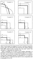
Graphically, the IMR is formed by all median rule segments. Figure 4 presents various examples for three-judge courts in a two-dimensional space. In each, for judges A, B, and C and their respective proper rules, the dotted line is the IMR, which is also a proper rule. Thus, in a case space, even in multiple dimensions, if all rules are proper, there exists a unique “median” rule. If all judges have proper rules, then they can always create a proper rule that has the same effect as hearing each case themselves.

Examples of Implicit Median Rules

Median Rules and Median Judges

It is possible that there will exist a true median judge, one whose rule is always more extreme than half the remaining rules and less extreme than half the remaining rules. Formally,

Definition. There exists a true median judge (judge

) with a {\bf true median rule} (rule

if and only if the judges can be ordered such that

. Proper rule

is a true median rule if and only if

.

In Figure 4, only example 4.2 shows a true median rule/judge. Note that the existence of a true median will be stable to small perturbations (unlike a multidimensional median in a policy space, which requires extremely precise symmetries of ideal points).

The IMR can exactly match the actual rule of one of the judges, and this will occur when a true median judge exists: Corollary 2. prop judge has imp med rule The Implicit Median Rule will be the rule of one of the judges if there exists a median judge a true median rule, so that judge

has proper rule

Interestingly, the IMR can also be the actual preferred rule of one of the judges even if her rule is not a true median rule. In example 4.4, Judge C is not a true median judge (and there is no true median rule), yet her preferred rule tracks the implicit median rule exactly.

However, the IMR need not actually be the preferred rule of any one judge—there will exist a median rule even without a median judge. (This again contrasts with the standard policy space, in that, if a policy-point median exists for an odd number of players, it must be one of the player's ideal points.) Furthermore, regardless of whether there exists a median judge with a true median rule, there will always be a local median rule and a local median judge for each range of cases defined by the segments of

. That is, for different regions of cases, different rules and judges are pivotal. In Figure 4, example 4.1, moving from left to right, judge B is first pivotal, then A, then C, then B again.

Assessing the Collegial Rule

For Kornhauser and Sager (1986, 91), “the principal measure of performance in preference aggregation is the ability of a particular process to reflect correctly the preferences of the members of the decision-making group,” which they call “authenticity.” By this measure, the implicit median (collegial) rule performs quite well, capturing majoritarian case outcomes perfectly. Moreover, we can expect consistency across similar cases. However, they distinguish consistency from “coherence,” which requires decisions to be “derivable from a unitary set of principles or embedded in some structured theory,” and they note that an amalgamated rule might not be derivable in this way even if the individual rules are (108, 111).

Because the amalgamation of proper rules is itself a proper rule, it will also be coherent to that extent. This stands in contrast with Easterbrook (1982) and Grofman (1993, 1757–77), which argue that we cannot expect consistency or coherence from collegial courts. On the other hand, even though the IMR induced by individual proper rules will always be a proper rule itself, this aggregated rule can still differ greatly in appearance and complexity. In examples 4.2 through 4.6, each individual judge has a conjunctive rule (a two-part test), such as a rational basis test, requiring a law challenged under the equal protection clause to be a rational means to a legitimate government end. The judges simply differ as to their preferred thresholds for meeting this test. Although the IMR is always a proper rule in these examples, it is not always a conjunctive test itself, as shown by examples 4.5 and 4.6. Thus, the aggregation of conjunctive rules need not yield a coherent conjunctive rule, and collegial doctrine can still differ from the jurisprudence of individual judges.⁷

Furthermore, perhaps not all proper rules are equally defensible philosophically. Perhaps, that is, some trade-offs between dimensions are defensible, and others are not. Perhaps some doctrinal structures are defensible, and others are not. Does “incoherence” only matter as a normative issue? If not, what are the implications of incoherence for compliance in the lower courts or the development of law? This paper suggests a framework with which to explore these issues.

I now move from a theory of rules to theories of rule making.

IMPLEMENTING COLLEGIAL RULES

If legal rules are the heart of judicial policy making, then battles over law are struggles over legal rules and over how they partition the case space. This section asks what rules can be implemented by self-interested judges as they come together to aggregate their preferences. There are two ways that judges on a collegial court make policy, through actual case decisions and through judicial opinions announcing general rules for deciding cases. I treat each in turn and then combine the two perspectives. Although proper rules have great intuitive and substantive appeal, most results below hold for extended rules more generally, and so I present results in terms of the ICR where possible (noting that this will be the IMR when all individual rules are proper rules).

Policy Making through Cases

Policy Making through Rules

Preferences over Rules. Suppose the collegial court does not hear all cases itself; rather, it announces a rule for lower courts to follow. As an extension to the general assumption made over case utility, I only assume that a judge strictly prefers rule C_y to rule C_z if the former yields all the same “correct” case disposition as the latter rule, and at least some additional region of “correct” dispositions. In effect, I only require that the judge prefer C^y to C^z if the former strictly dominates the latter as far as partitioning the case space, and I do not require any particular valuations over areas of the case space.

Formally, given the judge's preferred rule C_j, u_j(C_y)>u_j(C_z) if C_z⊂C_y⊂C_j or C_j⊂C_y⊂C_z. Otherwise, if there is a trade-off, either rule may be preferred. I need not and do not make assumptions as to how the judge resolves the trade-off, unless otherwise stated. This is a weak restriction on preferences, and so the results below are robust. (Parallels to the case preference assumptions noted above exist, and the fungibility assumption for utility over rules is shown in the Appendix.)

The Explicit Collegial Rule Game. In this preliminary version of a game over rules, I make two assumptions. First, the court votes over rules (by majority rule) and must announce a single rule, the explicit collegial rule (ECR). That is, no separate opinions are allowed (or at least any such opinions are ignored). Second, I assume this ECR is self-enforcing and automatically binds all subsequent case decisions, thus setting aside for now the problem of enforcement. This model is intended as a baseline for assessing the effects of modifying these assumptions to better capture actual judicial practice and institutions.⁹

In this game, is there an ECR that is stable under majority rule? Will the court cycle, or does the core exist?

Proposition 6. In the Explicit Collegial Rule Game

• a) under the fungibility assumption, if there is a true median rule, then it is in the core (and is itself the Implicit Collegial Rule);
• b) under the fungibility assumption, if there are only three judges, then the core is the Implicit Collegial Rule;
• c) if an explicit collegial rule is in the core, then it is the Implicit Collegial Rule;
• d) otherwise, cycling can occur.

That is, on larger collegial courts or where judges do not value all cases equally, there is generally no stable ECR. Any such ECR can be beaten by some other ECR by majority vote. If the judges made policy over a case space like legislators do, announcing a single binding statute (rule) as law, there can be cycling.¹⁰

However, the assumptions of this baseline model do not reflect current appellate court practice: judges and justices are permitted to write separate opinions, and their opinions are not self-implementing; rather, they are implemented through individual cases rising up the judicial hierarchy. The next step is to incorporate these features.

The Opinion Coalition Game. Suppose that each judge on the collegial court signs on to some opinion stating a rule to govern lower court decisions. This might be a coalition opinion supported by a majority, a plurality opinion, or even his or her own solo opinion.

How will lower courts decide cases when there is no majority opinion, in the shadow of fragmented opinions in the court above?¹¹

judges, or separate opinions/rules that show the support of at least

judges for this disposition.)

That is, suppose the lower courts obey the implicit collegial rule that would be induced by the announced set of rules, given the number of judges supporting each of them. (The next section shows why they should do so.) Let this be the \emph{Induced Implicit Collegial Rule}

(IICR). If there is a majority coalition behind a rule, then that rule becomes the IICR. Otherwise, it is cobbled together from those regions where a majority of announced rules overlap (just as the ICR itself is the majoritarian overlap of sincerely preferred rules).

Formally, an action for a judge in this game is the announcement of a rule, which may be the same rule as other judges (to form an opinion coalition). The set of rules announced yields the IICR, which in turn controls case dispositions and yields payoffs. The question is which rule coalitions will be stable (such that no judge will want to defect from her current position or current opinion coalition)? In equilibrium, can the IICR be the true ICR? In short, yes:

Proposition 7. rules coalition game In the Opinion Coalition Game, the true implicit collegial rule can be supported as the induced implicit collegial rule

as a Nash equilibrium. If a judge prefers to announce either his own preferred rule or the ICR when otherwise indifferent as to the rule he announces (i.e., case dispositions under the IICR are not affected by his choices), then the true implicit collegial rule is the only rule that can be supported as a Nash equilibrium.

Various specific opinions and coalitions are compatible with this, so long as the IICR is the true ICR itself (otherwise, the coalitions are not stable). Each of the following possibilities is, for example, equilibrium behavior:

1. Each judge writes separately, announcing his or her own (sincere) preferred rule.
2. Each judge joins an opinion announcing the ICR.
3. A combination of these two strategies, so that each judge in the majority in the current case announces the ICR and others announce their sincerely preferred rules in dissent or separate concurrences.

Therefore, although requiring a single, binding ECR can lead to cycling, the possibility of writing separately means that the true ICR will be stable against individual defections and that rules other than the ICR are vulnerable to such defections. Indeed, note that it is a weakly dominant strategy to announce ones own preferred rule.

So far, this assumes that lower courts simply obey the IICR. One final result, bringing individual case decisions back in, shows why they should do so.

Enforcing Legal Rules

When an appellate court announces a legal rule in a formal opinion, the game does not end there. The judges on that appellate court can themselves hear appeals in the very cases decided under that rule. How does this affect collegial rule-making?

Oliver Wendell Holmes defined law as “the prophecies of what the courts will do in fact, and nothing more pretentious” (1897, 460). To meet this standard, a meaningful legal rule must predict how courts will actually decide cases. Segal and Spaeth (2002) agree with Holmes's emphasis on prediction, arguing that we should pay more attention to what justices do than to what they say—but this raises an important question. Can we use what they say as a guide as to what they will do? When will a rule announced by a collegial appellate court actually be “law” in the Holmesian sense? When will it predict how the appellate court will decide cases on appeal?

Call a legal rule enforceable if it correctly predicts how the collegial appellate court will decide the cases it reviews after that rule is applied. Consider a game in which the court decides a case by majority vote, announces a legal rule or rules, and then decides another case in the same issue area by majority vote. Then, the following result holds: Proposition 8. The only enforceable legal rule is the Implicit Collegial Rule.

If an appellate court states a legal rule other than the ICR, or if the rule induced by a set of opinions is other than the ICR, the judges face a commitment problem. Any case that would be decided in contradiction to the ICR can be reversed by majority vote on appeal, undercutting any incentive to logroll in the first place. In any such case, a lower court could evade the “official” rule and simply follow the ICR, knowing that a majority of justices support that act of noncompliance. In fact, a lower court following the “official” rule would be subject to reversal on appeal.

Setting aside further complications, the lower courts thus have little incentive to apply a rule other than the ICR, and so the higher court has little incentive to issue a divergent rule in the first place. Although appellate review can help a higher court control a lower court, it also creates a commitment problem for logrolls and undermines the implementation of any rule other than the ICR.

Possible Restrictions on Utility over Rules:

These are parallel to the case-utility assumptions. The fungibility assumption requires that the judge only care about the percentage of the case space that is correctly partitioned. For proper rules, in one dimension, this would the distance between the preferred rule and the ECR cut-point r*: −|r*−r_j|. In two dimensions, the utility loss is the area between the curves (

). In more general spatial terms, this loss is the hypervolume of cases incorrectly decided. Meanwhile, the proximity assumption would allow the judge to care more about some regions of the case space than others, depending on how close they fall to the indifference set marked out by the preferred proper rule. This would require an integral weighted by a salience term.

Cycling over ECRs can occur: Example 2 (Variable utility and voting over rules).}\,\,{Consider Example 1 above. Let rules r_a, r_b, and r_c be equivalent to

, except for deciding bundles of cases surrounding x¹ and x² as {1, 1}, {0, 1}, and {1, 0}, respectively. Then cycling can occur as above, with

.

Proof of Proposition 6. (a) Suppose the ICR is not in the core. Then, there exists a rule

that beats the ICR outcome set

under majority rule, so that at least a majority of judges strictly prefer

. The proof from this point is similar to that of Lemmas 2 and 3, focusing on the percentages of cases in each of the four categories instead of the cardinalities of sets of cases. (b) The proof follows that for Lemma 2. (c) The proof follows that for Lemma 1.

Proof of Proposition 7. First, note that there are Nash equilibria in which the IICR is the true ICR, so that

. Specifically, if every judge supports his or her own rule or the ICR, then

. There is no incentive to defect, because if judge j is pivotal for some set of case outcomes, a shift away from supporting C_j or

can only lead to the wrong case outcomes under C_j. (If judge j is not pivotal, there is obviously no reason to defect.) Given the indifference assumption, to show that only the true ICR can be supported, suppose otherwise and consider an arbitrary judge j not announcing her preferred rule. If her rule is not pivotal in any case (if the induced collegial rule does not change), she will announce her sincere rule or the ICR. If her announced rule is pivotal in any set of cases, then defecting from it to her preferred rule increase the set of “correct” dispositions. No matter what the other judges announce, a sincere announcement of C_j is a weakly dominant choice.

Proof of Proposition 8. Working backwards, Proposition 5 shows that any subsequent case outcomes following the announcement of a legal rule will be controlled by the ICR (as must be the case in period 1). Thus, only the ICR is enforceable.