

A large part of the human language experience involves face-to-face encounters between speakers, so physical space is a crucial aspect of language variation and change. Nerbonne and Kleiweg's (Reference Nerbonne and Kleiweg2007) Fundamental Dialectological Postulate states that “geographically proximate varieties tend to be more similar than distant ones” (cf. Bloomfield's principle of density [1933:476]). This notion is supported by dialectometric investigations of well-known languages such as German and Norwegian, which consistently show strong correlations between geographic distance and dialect variation (Kretzschmar, Nerbonne, Opas-Hanninen, & Bounds, Reference Kretzschmar, Nerbonne, Opas-Hanninen and Bounds2010; Nerbonne, Reference Nerbonne2010; Nerbonne & Heeringa, Reference Nerbonne, Heeringa, Auer and Schmidt2010). But what happens when dialectometry is applied to a small, non-Western, nonindustrialized, clan-oriented, indigenous language community such as the Sui people of southwest China?
INDIGENOUS MINORITY PERSPECTIVES ON LANGUAGE VARIATION AND CHANGE
Indigenous minority languages have provided important insights in many areas of linguistics, including phonetics, phonology, morphology, syntax, typology, anthropological linguistics, and other subfields of linguistics. However, such languages have been noticeably underrepresented in the research paradigm of language variation and change. Many contemporary principles in this field are primarily based on majority language communities or large, well-known minorities, rather than indigenous minorities.
Due to rapid globalization, many indigenous languages are facing acute contact and pressure from majority societies. When such communities begin to blend into dominant societies around them, there is a significant loss of diversity. Opportunities for observing indigenous sociolinguistic practices vanish along with each community. Even when a handful of scattered speakers of a language remain, the indigenous sociolinguistic interactions of daily community life can never be observed in the same way again. With this in mind, Stanford and Preston (Reference Stanford and Preston2009) encourage a new wave of research to focus on as many indigenous minority communities as possible while they are still viable.
Underrepresented communities can offer many new perspectives on language variation and change (Nagy & Meyerhoff, Reference Nagy, Meyerhoff, Meyerhoff and Nagy2008; Sankoff, Reference Sankoff1980; Stanford, Reference Stanford2007c). Certain sociolinguistic factors that have been important in majority groups may be less relevant in indigenous groups, whereas other factors, such as clan affiliations, may be crucial (Stanford & Preston, Reference Stanford and Preston2009:6–12). For example, although socioeconomic status holds an important role in contemporary sociolinguistic principles (Labov, Reference Labov1994, Reference Labov2001), many rural indigenous societies such as Sui are relatively egalitarian, making such distinctions less relevant. Yet the linguistic construction of society and personal identity may be observed in other aspects of such communities (e.g., Clarke, Reference Clarke, Stanford and Preston2009).
SPACE
Space is another factor for which indigenous languages have new insights to provide. What can indigenous minority communities show us about language variation and space? The present study helps answer this question by applying dialectometry techniques to Sui. The study not only provides new results about Sui and indigenous languages in particular, but also new perspectives about the overall role of space and place.
Generalizations about physical space can provide approximate predictions in the form of averages across large populations, such as Nerbonne and Kleiweg's (Reference Nerbonne and Kleiweg2007) Fundamental Dialectological Postulate. Nerbonne and Kleiweg characterize this notion as a statistical tendency emerging from many different studies, rather than an absolute law (p. 154; cf. Bloomfield's principle of density [1933:476]). Many studies seek broad generalizable patterns across large populations, including comprehensive regional studies such as the Atlas of North American English ([ANAE] Labov, Ash & Boberg, Reference Labov, Ash and Boberg2006; cf. Kurath, Reference Kurath1939) and dialectometric analyses (e.g., Nerbonne, Reference Nerbonne2010). Such studies often attempt to represent most or all of a society, and they often find significant large-scale patterns that generally support the Fundamental Dialectological Postulate. In fact, simple geographic distance typically accounts for 16% to 38% of variation (Kretzschmar et al., Reference Kretzschmar, Nerbonne, Opas-Hanninen and Bounds2010; Nerbonne, Reference Nerbonne2010; Nerbonne & Heeringa, Reference Nerbonne, Heeringa, Auer and Schmidt2010).
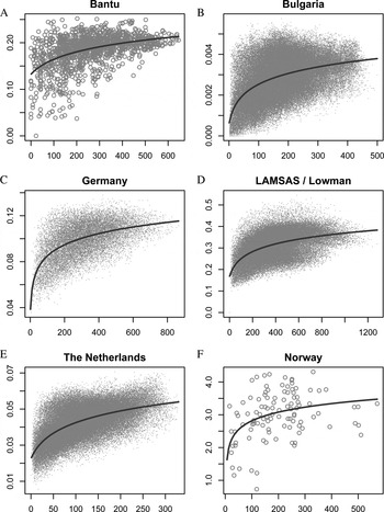
Dialectometry provides remarkably consistent large-scale results. Seguy ([Reference Seguy1971] cited in Nerbonne, Reference Nerbonne2010) found that the correlation between geographic distance and dialect difference is usually sublinear, so the common appearance of this sublinear curve has been called Seguy's Curve (Kretzschmar et al., Reference Kretzschmar, Nerbonne, Opas-Hanninen and Bounds2010; Nerbonne, Reference Nerbonne2010:3823). This sublinear (logarithmic) curve is exemplified in Figure 1, where Nerbonne's (Reference Nerbonne2010:3825) graphs are reprinted for comparison with the Sui results to be presented in the current study. The figure shows Nerbonne's (Reference Nerbonne2010) dialectometric analyses of Bantu, Bulgaria, Germany, the United States, the Netherlands, and Norway. Note the logarithmic trend lines fitted to the data in each case. Naturally, there is a considerable amount of statistical variance in all such studies, owing to innumerable localized social, historical, and political factors, as well as individual variation. Nonetheless, the impressive overall consistency of these geographic correlations across many languages shows that dialectometry can capture meaningful linguistic generalizations and very strong correlations between dialect differences and simple geographic distance.
Nerbonne's graphs of geographic distance in kilometers (x axis) versus dialect differences (y axis). The y axes have different scales, but they all represent relative dialect differences. Each point represents a paired comparison of geographic distances and dialect differences. For example, the geographic distance between Location A and Location B is plotted against the dialect difference between those two locations, then the distance between Locations A and C is plotted against the dialect difference between Locations A and C, and so on. Reprinted, with permission, from figure 2 on page 3825 of Nerbonne, John. 2010. Measuring the diffusion of linguistic change. Philosophical Transactions of the Royal Society B 365:3821–28.

THE PRESENT STUDY
This study tests whether the broad generalizations and methods of dialectometry can be meaningfully applied to a small, clan-based indigenous society. In Figure 1, note the large scales of geographic distance (maximum distances of 300 km to 1200 km) that are typical for most dialectometric studies. By contrast, the current Sui dialectometry study has a maximum geographic distance of only 55 km, yet this area represents a large proportion of Sui society.
Because the Sui people are largely concentrated in one relatively small region of China, it is possible to take an “encompassing” perspective on dialect patterns across most of Sui society, that is, covering the major geographic region of the society like ANAE covers North America. Located in a compact region in southwest China, Sui is apparently the smallest society to be studied with dialectometry.Footnote 1 At the same time, because Sui society is geographically tiny compared to most prior work in dialectometry, it is possible to look more closely at local particulars, that is, the social meaning of place (e.g., Johnstone, Reference Johnstone and Fought2004, Reference Johnstone and Mesthrie2011). Therefore, this study can draw strength from both the generalized perspective as well as a local, particularized perspective. Will the Sui dialectometry results be consistent with the Fundamental Dialectological Postulate and consistent with dialectometry results from larger societies? Or will the particulars and social meanings of place in this small, indigenous society make such generalizations unattainable or meaningless? For example, clan identity is a major factor in multidialectal Sui villages (Stanford, Reference Stanford2008a, Reference Stanford2008b, Reference Stanford2009a, Reference Stanford, Stanford and Preston2009b). Sui women leave their own clans and move permanently to the husband's village at the time of marriage, so it could be that the very notion of a regional “data point” on a map is not relevant. Owing to exogamy, every Sui village includes speakers with a wide range of clan dialects. Will it be meaningful to plot geographic data points in this context? Perhaps not. Yet Labov suggested, “As always, it is good practice to consider first the simpler and more mechanical view” (2001:506; cf. Trudgill, Reference Trudgill2008:251). Therefore, the “mechanical” dialectometric approach should be tested in such a society.
With these considerations in mind, the following hypothesis will be tested:
Hypothesis: Dialectometry will not produce effective results for Sui because this indigenous, clan-based society occupies only a very small geographic region, and it has many local cultural and sociolinguistic issues that differ dramatically from societies previously studied with this methodology.
RESEARCH BACKGROUND
Different Scales, Same Principles?
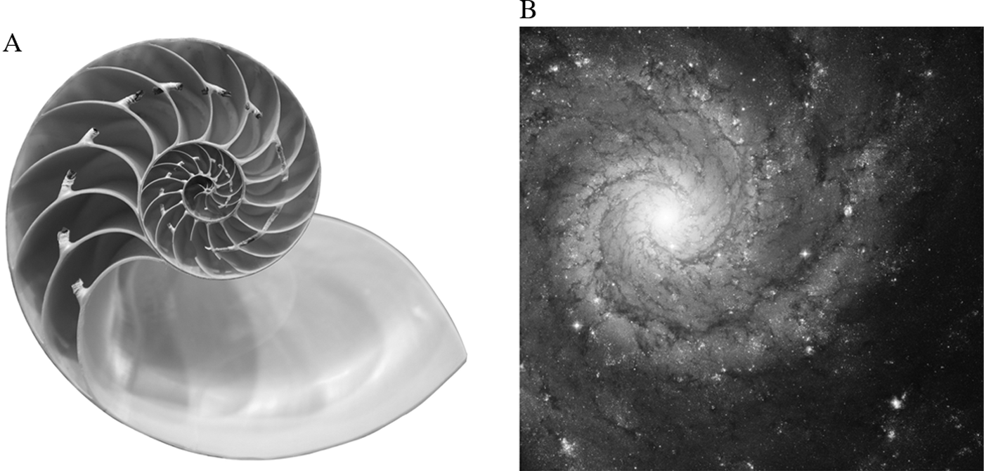
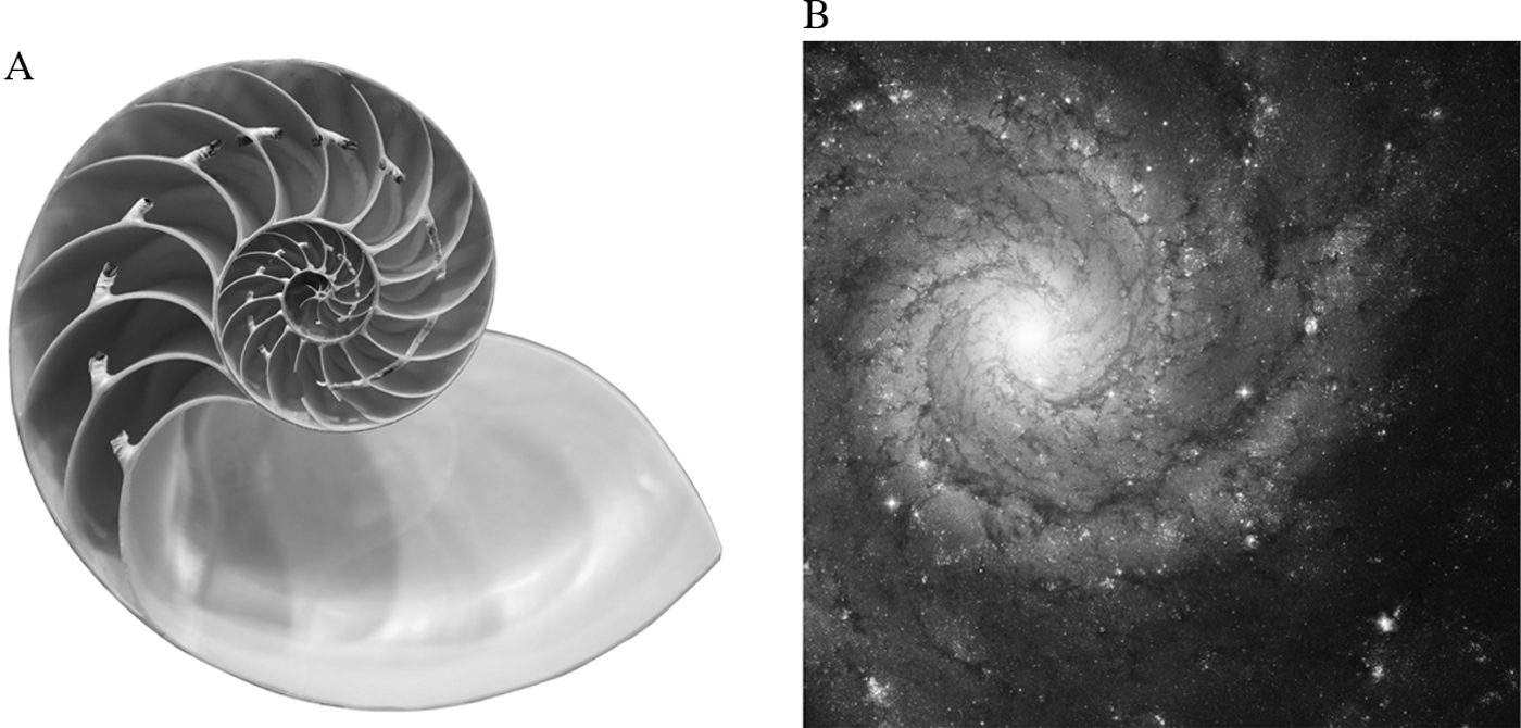
Can dialectological methods be applied to both large and small societies with equal effectiveness? In the natural world, a pattern is sometimes observed on very different levels of scale. The elegant spiral shape of a nautilus shell is strikingly similar to the far larger spiral of a hurricane or a spiral galaxy in space (cf. Darling, Reference Darling2004:188–189; Livio, Reference Livio2002). Underlying mathematical principles are operating on different levels of scale to produce those familiar forms of spiral geometry in nature. Perhaps dialect principles can also operate on different levels of scale. The ANAE recorded speakers representing vast stretches of North American society, which occupies approximately 9.4 million square miles and had a population of over 248 million people in the United States and major cities of Canada at the time (Labov et al., Reference Labov, Ash and Boberg2006:31). The present study of Sui also recorded representative speakers across a society, but Sui society is dramatically smaller than North American society in population and geography. The present study examines a region of about 780 square miles representing approximately 180,000 speakers, the bulk of Sui society.Footnote 2 This Sui project is therefore categorically smaller in scope than ANAE, yet proportionally comparable in terms of representing a society.
In other work, small geographic regions have shown clear linguistic patterns that correlate with physical space. Chambers and Trudgill examined Brunlanes, Norway (1998:177–179; cf. Trudgill, Reference Trudgill1974) and found that dialect contrasts among villages in that tiny 13-kilometer-wide region can be explained by principles of dialect diffusion. Similarly, German villages in a tiny region within the larger “Rhenish Fan” have distinctive dialect features despite their close proximity, a result that can be interpreted in terms of the notion of residual zones (Chambers & Trudgill, Reference Chambers and Trudgill1998:92–93). In addition, among Yami speakers of Orchid Island, Taiwan, there is a clear isogloss for vowel-raising across the tiny island (Rau, Chang & Dong, 2009:277).
For many small regions, it is important to investigate highly localized social meanings, rather than simply applying the principles of dialectology as found in larger regions. Labov's (Reference Labov1963) study of the small island of Martha's Vineyard showed geographic contrasts in two variables, (ay) and (aw), but also uncovered important factors of social identity. Becker's (Reference Becker2009) study of the pronunciation of /r/ in a small region, the Lower East Side of New York City, showed how residents construct a highly localized neighborhood “place identity.” Hill's (Reference Hill and Terrell2001) investigation of the Tohono-O'odham people of Arizona suggested that large-scale dialect geography studies of majority groups are not always compatible with small, indigenous groups. She advocated an anthropological dialectology that is sensitive to particulars of small indigenous populations. For the indigenous Tarascan society in Mexico, Friedrich (Reference Friedrich and Edmonson1984, Reference Friedrich and Friedrich1979[1971]) coined the term pueblo dialectology. As discussed herein, some aspects of the present Sui study might be viewed as a case of “rice paddy dialectology.”
In terms of dialectology, then, what is the difference between a large community and a small community? Frequency of contact and physical separation of speakers are clearly important in this respect. Despite the rise of Web-based social media, a very large amount of human language interaction continues to depend on face-to-face interactions. Small overall geographic range and small population size naturally mean that there is greater likelihood of close contact between any two given speakers, all other things being equal. Smaller regions also have a greater likelihood of kinship relationships, which can affect frequency of contact as well. Sui society has all of these traits of a small society.
The Sui People
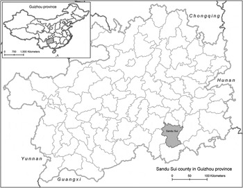
The Sui people (pronounced [sʊi]) are concentrated in a small rural region in Guizhou province, southwestern China. Ninety-three percent of the Sui people live in Guizhou (Wei & Edmondson, Reference Wei, Edmondson, Diller, Edmondson and Luo2008:585), and the cultural and linguistic center of the ethnic group is Sandu Sui Autonomous County, located in the southern part of Guizhou. According to the 2000 census, 189,128 Sui people lived in Sandu County (Castro, personal communication; China National Bureau of Statistics, 2003). The location of Guizhou province and Sandu County is shown in Figure 2.
Sandu Sui Autonomous County in Guizhou Province, China. Map source: Evans Map Room, Baker/Berry Library, Dartmouth College/lmh. Data sources: DIVA-GIS, Stanford, Linguistics Department, Dartmouth College.

Sui Villages
Rural Sui villages maintain a traditional agricultural lifestyle and distinctive cultural practices. For example, rural women wear bright blue or green traditional Sui clothing on a daily basis, and the community has a vibrant annual Sui New Year festival. Patrilineal clan exogamy is strictly practiced, and the wife is expected to marry into the husband's village. Clan ideology is constructed through these exogamous practices and locals’ understanding of lineage. Surnames are passed from father to child and maintained for life. Therefore, in a given village, all the men, children, teenagers, and unmarried women share the same surname.
The Sui Language
Sui is a member of the Tai-Kadai family. The language is tonal and largely monosyllabic (Burusphat, Wei, & Edmondson, Reference Wei, Edmondson, Diller, Edmondson and Luo2003; Diller, Edmondson, & Luo, Reference Diller, Edmondson and Luo2008; Edmondson & Solnit, Reference Edmondson and Solnit1988). An unpublished 1956 manuscript, Shuiyu Diaocha Baogao (henceforth SDB), is an early dialect geography study of the region. Other early work includes Li (Reference Li1948, Reference Li1965) and Zhang (Reference Zhang1980). Recent Sui research includes Zeng and Yao (Reference Zeng and Yao1996); Edmondson, Esling, Harris, and Wei (Reference Edmondson, Esling, Harris and Wei2004); Castro (Reference Castro2011); Wei (Reference Wei2011); Stanford (Reference Stanford2007a, Reference Stanford2007b, 2007d, Reference Stanford2008a, Reference Stanford2008b, Reference Stanford2009a, Reference Stanford, Stanford and Preston2009b, Reference Stanford2011); and Stanford and Evans (Reference Stanford and Evans2012).
In rural Sui villages, daily conversation between Sui people is overwhelmingly conducted in Sui. Many Sui people can also speak Chinese (Southwest Mandarin), although older women tend to be monolingual in Sui. Chinese loanwords are observed in educational and political contexts, and some other words have been borrowed from Chinese recently and in earlier eras (Stanford & Evans, Reference Stanford and Evans2012; Zeng, Reference Zeng2004). Chinese characters are used for written communication.Footnote 3
Sui speakers do not consider any particular Sui dialect to be more prestigious or preferable, and there are no known sociohistorical, political, or economic reasons for any dialect to be perceived more positively or negatively than others. Some scholars have traditionally treated one Sui dialect (Sandong Sui) as a standard (e.g., Luo, Reference Luo1992; Zeng & Yao, Reference Zeng and Yao1996), but there is no ideology of a “standard Sui dialect” in Sui folk linguistics.
Sui Tones
Six lexical tones of Sui are shown in Table 1, representing a village in the Sandong region (Stanford, Reference Stanford2008a; Zeng & Yao, Reference Zeng and Yao1996). Following Chao's (Reference Chao1930) 1 to 5 pitch scale, a mid-level tone is represented by 33, whereas 53 represents a high-falling tone, and so on. Superscripts represent tone numbers, for example, [qa1] ‘to read’ indicates the syllable bears Tone 1.
Tones in Sandong Township for unchecked syllables

Some regions pronounce Tone 6 as 24 rather than 55, and there is some slight regional variation in Tone 1 (Stanford, Reference Stanford2011). Recent loanwords with Mandarin Tone 3 are produced as 55 in Sui (Stanford & Evans, Reference Stanford and Evans2012). In addition to the unchecked tones in Table 1, tones of checked syllables are numbered as Tones 7 and 8 (see Stanford, Reference Stanford2008a, for a description).
Methods
The dataset for the present study was collected during fieldtrips in August 2010, August 2006, and August 2005. Further background on the Sui language and culture is based on the author's four years in Guizhou, including time spent learning the language.
Locations
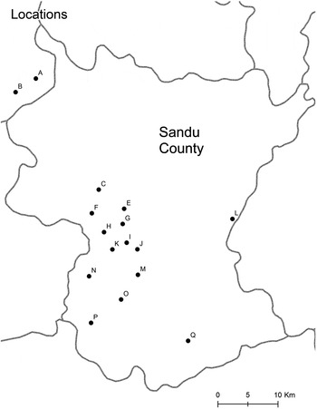
The locations represented in the study are shown in Figure 3. Similar to the locations sampled in SDB (1956), the locations sampled in the present study represent most of the primary populated Sui areas in the region. Like SDB, the region just west of Location L was not sampled because it is a mountainous, sparsely populated area. Similarly, neither SDB nor the present study sampled the less-populated mountainous region between Location C and Locations A and B. The locations in this study are a representative sample of the heart of the rural Sui language and culture.Footnote 4
Locations of the present study. Map source: Evans Map Room, Baker/Berry Library, Dartmouth College/lmh. Data sources: DIVA-GIS, Stanford, Linguistics Department, Dartmouth College.

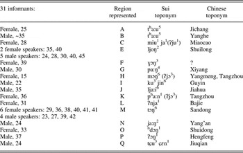
The informants and their representative locations are listed in Table 2. For Locations E and M, multiple speakers were available from a prior study (Stanford, Reference Stanford2008a). Even though it would be ideal to conduct a study of multiple speakers in each location, this was not always possible due to fieldwork limitations. In fact, however, prior Sui work shows that individual speakers (both women and men) are very reliable representatives of their home dialect regions. Detailed investigations (Stanford, Reference Stanford2008a, Reference Stanford2008b, Reference Stanford2009a, Reference Stanford, Stanford and Preston2009b) show that both female and male Sui speakers consistently produce the regional features that represent their home clans; they use these features to continually index and construct loyalties to their home communities.
Informants and locations represented in the present study

Note: All ages given in years.
The Sui language place-names in the table are given as provided by Sui speakers; some represent village-level names, whereas others represent larger areas. Location D is omitted for the present study because that informant's data only contained half of the words in the list.
Coordinates of the villages were located in Google Earth, and then transferred to geographic information system mapping software according to longitude and latitude (Evans Map Room, Dartmouth College). For cases where the specific village locations were not available in Google Earth (H, K, N), a Sui consultant marked a map with the most likely locations.
Age
Following SDB (1956), the targeted demographic was middle-aged and young adults. SDB had an age range of 22 to 46 years old, with the exception of a 17-year-old. The age range in the present study was 22 to 45 years old, with the exception of one 15-year-old.
Gender
Gender poses a methodological challenge for any dialect geography study of a clan exogamous society. Because rural Sui women typically marry at a young age (late teens or early 20s) and move to the husband's village, most adult women are not living in their home villages. The SDB (1956) project was conducted during the era of traditional dialectology, so SDB focused primarily on men (15 men and 1 woman). The present study sought a balance of women and men (15 women and 16 men) in order to avoid a narrow perspective on Sui dialects.
Dorian (Reference Dorian2010:309) pointed out that traditional dialectology's focus on male informants is especially problematic for indigenous minority communities, and Sui is a case in point. For example, one Sui village of 35 households (~150 people) included in-married wives representing 19 different clans. Dialectometry and dialect geography unfortunately miss this level of complexity in Sui sociolinguistics. In fact, due to the very nature of dialect geography, any study of regional variation in a patrilocal clan exogamous society runs the risk of overlooking the importance of women's speech. Yet, as discussed in the Conclusion section, in-married women have crucial roles in Sui variation and change, especially with respect to long-term diffusion and contact.
Even so, ethnographic discussions show that Sui people have a clear, emic sense that each village has one particular variety that is the “home dialect.” This dialect is invariably the clan dialect of the men and grown children. It is therefore analytically meaningful to investigate Sui villages under the assumption that a single dialect represents a given village from a certain point of view, even while recognizing the actual linguistic complexity of in-marriage and contact. Field observations, ethnographic interviews, and prior research all suggest that this interpretation is a reasonable heuristic. Although dialect contact is a fact of daily life, each village has a dominant dialect that is apparently quite stable and is passed on to each new generation born into that village (Stanford, Reference Stanford2008a, Reference Stanford2008b, Reference Stanford2009a, Reference Stanford, Stanford and Preston2009b).
Mobility
For the purposes of dialect geography, it is usually preferable to record permanent, lifelong residents in their hometowns. For 11 of the recordings, interviews were conducted in the informant's home village or very nearby (Locations E, I, J, M). In other cases, however, it was necessary to record informants who had moved away from their home villages. Three issues were involved. First, there is the methodological challenge of in-marriage. Because most rural Sui women traditionally marry at a young age and move to the husband's village, it is difficult to find adult women who remain in their original home villages. At the same time, this system of clan exogamy has the positive effect of providing opportunities to interview women from regions that would otherwise be difficult to reach. Locations A, F, H, K, L, and O were represented by women who were raised to adulthood in those locations and had in-married to other villages. Those women were recorded in their places of adult residence (husband's village). Locations E and M were represented by both men and women: men who were lifelong residents of E and M, and women who were raised to adulthood in E and M and had in-married to other villages, where they were recorded.
Second, it was not possible for the author personally to visit all of the regions represented here. In keeping with Sui customs, the author develops his research contacts through personal friends and their own kinship connections. The author has contacts in many but not all Sui regions, and it would be culturally inappropriate (especially as a Westerner) to randomly approach Sui people for interviews (Stanford & Preston, Reference Stanford and Preston2009:16).
Third, modern Sui society is becoming more mobile; even rural villagers are finding opportunities for work in locations beyond their original home villages, and others become teachers in nearby small towns. Locations Q, P, N, G, and C are represented by speakers who had moved to a local town (Zhouqin). Location B is represented by a speaker who was a migrant laborer recorded in the city of Duyun, north of the Sui region.
The strong clan ideology of Sui communities is actually quite helpful with respect to these issues of mobility. The influence of mobility on dialect features appears to be quite limited in this society, as speakers place great importance on loyalty to their original clans—their communities of descent (Stanford, Reference Stanford2009a). Prior research shows very clear evidence that Sui speakers carefully maintain linguistic loyalty to their original clan dialects regardless of mobility later in life. In Stanford's (Reference Stanford2008a) quantitative, acoustic analysis of the phonological features of in-married women, the women maintained their original clan dialect features to a very high degree, despite a decade or more in the husband's village. Lexical variables followed the same pattern: In recordings of free speech in different regions, in-married women produced the variant of their original clan dialects in all 226 recorded instances of regional lexical variables (Stanford, Reference Stanford2009a). As for ethnographic interviews, Stanford (Reference Stanford2009a) found that Sui speakers express a very strong loyalty to their original clan dialects. Speakers are continually constructing and maintaining their clan identities through stable linguistic choices, regardless of in-marriage or other mobility.
The following quote is from a Pan-surnamed woman who had in-married into a Lu-surnamed village. She had been living in her husband's village for over a decade, and she described the village's dialect contact situation as follows: “They are surnamed Lu, so they say ɛi [1st Sg]. We are surnamed Pan so we say ju [1st Sg]. Each speaks their own way. . . . People surnamed Lu speak like the Lu place. We people surnamed Pan speak like people surnamed Pan” (Stanford, Reference Stanford2009a:295). In fact, speakers report that an in-married woman would be ridiculed or criticized if she used the local dialect features of her husband's village, rather than her original clan dialect.
Finally, note that Stanford's (Reference Stanford2011) 50-year real-time dialect geography comparison in this region finds a high degree of dialect consistency over time, despite the interpersonal dialect contact occurring through the social system of clan exogamy. Naturally, there are likely to be subtle, unnoticed, long-term communal changes happening as a result of such clan contact. But those changes would be very slow—longer than the 50 years examined in Stanford (Reference Stanford2011).
Interviews
The author used spoken Sui to elicit a list of 113 words from each informant. Some speakers did not produce a few of the words, so the dataset consists of 90 to 113 words per informant. Following Chambers (Reference Chambers1992) and related work, the target words were elicited through identification of pictures and actions, counting, and antonyms (such as “This dog is big. That dog is ___.”). This produced a semiconversational speech style. Interviews were recorded with a digital recorder, Edirol R-09HR (for Locations E and M, recordings were digitized from an analog Marantz recorder). The interview was designed to be appropriate in monolingual Sui in order to include older Sui women who might not speak Chinese. Chinese was used occasionally with a few informants who were bilingual in Chinese and Sui.
It should be noted that the Sui dataset is not taken from a random text. The word list was developed through the author's long-term observations of common words and dialect differences during his fieldwork and learning Sui over several years. The interview list focuses on concepts that can be easily communicated with pictures or simple actions/objects, including a broad range of linguistic features from interview activities such as pointing to simple body parts; actions such as standing, sitting, and counting; pictures of cooking utensils, types of food, animals; and so on. In this way, the dataset covers a wide range of semantic fields found in everyday conversation. The interview list also targeted specific words that were likely to show regional contrasts, such as dialect contrasts in Tone 6, diphthong variables, and lexical variables like first singular. The dataset therefore serves as a broad-based, representative sample of everyday Sui conversational language as used across the region, but one should also keep in mind the possible influence of particular words in the word list.
Dialectometry Methods
The methods of dialectometry applied in this study are based on Gooskens (Reference Gooskens2005), Gooskens and Heeringa (Reference Gooskens and Heeringa2004), Heeringa and Nerbonne (Reference Heeringa and Nerbonne2001), Kretzschmar et al. (Reference Kretzschmar, Nerbonne, Opas-Hanninen and Bounds2010), Nerbonne (Reference Nerbonne2009, Reference Nerbonne2010), Nerbonne and Heeringa (Reference Nerbonne, Heeringa, Featherston and Sternefeld2007, Reference Nerbonne, Heeringa, Auer and Schmidt2010), and Nerbonne and Kleiweg (Reference Nerbonne and Kleiweg2007). In addition, dialectometry studies in Chinese area linguistics are considered as well (Cheng, Reference Cheng1997; Tang & van Heuven, Reference Tang and van Hueven2009; Yang & Castro, Reference Yang and Castro2008). All of these studies explore how aggregate measurements of dialect features can be correlated with geographic distance. In the dialectometry literature, there are open questions about some aspects of methodology, including the fact that there are “myriad plausible techniques” for calculating dialect differences (Nerbonne & Kleiweg, Reference Nerbonne and Kleiweg2007:152, 2010). Yet this body of literature provides impressive support for the overall notion that dialect difference and geographic distance have a strong correlation (recall Figure 1).
The notion of quantifying regional dialect differences follows Seguy ([Reference Seguy1973] cited in Chambers & Trudgill, Reference Chambers and Trudgill1998:137). Many studies have explored the use of Levenshtein Distance, also called String Edit Distance (Levenshtein, Reference Levenshtein1966, cited in Kruskal, Reference Kruskal, Sankoff and Kruskal1999[1983]; see also Heeringa, Reference Heeringa2004:121). Levenshtein Distance is a calculation of “the least expensive means of transforming one sequence into another” (Nerbonne & Kleiweg, Reference Nerbonne and Kleiweg2007:151). Example (1) illustrates the basic idea using Gooskens and Heeringa's (Reference Gooskens and Heeringa2004) calculation for two pronunciations of afternoon: [æəftənʉn] and [æftərnʉn].

The total cost of 3 is then divided by the word length to produce a dialect difference score. Other algorithms are similar, although there are different viewpoints on the details, for example, should a substitution have a cost of 1 or 2 (1 for deletion plus 1 for insertion)? With respect to such issues, Nerbonne and Kleiweg (Reference Nerbonne and Kleiweg2007) pointed out that the field of dialectometry currently has an “embarrassment of riches.” There are different ways to calculate dialect differences, and questions remain about which approach is most effective. Because the goal of this study is to test the general effectiveness of dialectometry in Sui culture, the present study takes a fairly generic Levenshtein approach, following the basic model in (1) and adapting it for Chinese area linguistics.
Applying dialectometry to Sui
Because most prior work in this paradigm has involved European languages, some modifications are necessary for a tonal, monosyllabic language like Sui. Analyzing Chinese dialects, Cheng ([1997] cited in Tang & van Heuven, Reference Tang and van Hueven2009)Footnote 5 counted a cost of one point for each of the following: onset, glide, nucleus, coda, and tone. The present study takes the same basic approach but merges the onset and glide into a cost of one total point. In this way, different Sui dialects can be compared consistently with respect to the nucleus. A single Sui syllable therefore has a total of four possible points: onset, nucleus, coda, and tone. This raises the question about whether one particular element should be weighted more than another, for example, tones versus segments. With regard to this question, Cheng (Reference Cheng1997:55) pointed out that it is best to assume equal weights until future work establishes a firm basis for different weights between segmental and tonal phonology.
With 16 locations, this Sui study is comparable in size to the SDB (1956) Sui dialect geography study, and it is also comparable to the 15 locations analyzed for Norwegian dialectometry (Gooskens & Heeringa, Reference Gooskens and Heeringa2004; Nerbonne, Reference Nerbonne2010:3825). This Sui study does not have the scope of geographic data points available in large-scale studies, such as the massive Linguistic Atlas of the Middle and South Atlantic States (cf. Kretzschmar, Reference Kretzschmar2009). This exploration of Sui dialectometry provides meaningful results proportional to the scale of the society, and it opens the path for future research in other small rural indigenous communities.
Note that the use of these 16 discrete locations is not intended to suggest that Sui dialects necessarily have discrete boundaries or simple, categorical, geographic lines between dialect features. As Britain pointed out, the isoglosses and boundaries of traditional dialect geography have sometimes been criticized as wrongly implying “abrupt, discrete, and invariable” contrasts among dialect regions (2002:629; cf. Kretzschmar, Reference Kretzschmar2009:66ff; Nerbonne, Reference Nerbonne2009:187–189). The 16 Sui locations are windows into a far more complex sociolinguistic reality. Nonetheless, the data from these locations can provide valuable measurements of some of the properties of Sui regional variation, just as studies such as ANAE have provided valuable new knowledge about American English (Labov et al., Reference Labov, Ash and Boberg2006).
Calculating dialect differences in Sui
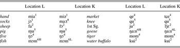
First, dialect differences were calculated from the database of dialect data. Two of the locations had more than one speaker (E and M). Because the other locations were represented by one speaker per location, the results of the multiple-speaker locations were averaged so that those locations had the same weight, that is, one speaker. Table 3 provides examples of data elicited in two locations.
Example words from two locations of the study

Note: Tone “6H” refers to the high 55 value of Tone 6; Tone “6L” is the low 42 value.
Dialect distances for each location were calculated using two different methods. As noted, there are several different possibilities for calculating dialect distance. For this study, two approaches were used:
1. Combined Index: In this approach, each item has a total possible score of 4 (i.e., 1 point for onset, 1 for nucleus, 1 for coda, 1 for tone), regardless of whether the items involved lexical or phonological variables (cf. Cheng, Reference Cheng1997). For example, the word market is pronounced [tɕe4] in Location C but [qe4] in Location M. This word scores 1 point due to the different onsets [tɕ-] and [q-]. The word head is pronounced [ku3] in Location C but [qam4] in Location M, thereby scoring 4 points (onset, nucleus, coda, tone are all different). The overall dialect distance is then computed by taking the total score and dividing by the total possible points.
2. Lexical/Phonological Index: This approach is based on Seguy's notion of weighting each type of variation equally (Chambers & Trudgill, Reference Chambers and Trudgill1998:137–140). In this study, lexical variables are treated separately from phonological variables (cf. Spruit, Heeringa, & Nerbonne, [Reference Spruit, Heeringa and Nerbonne2009], for an analysis of different linguistic levels in Dutch). Specifically, a lexical index is calculated by dividing the total score of the lexical variants by the total lexical variables. A phonological index is calculated by dividing the total score of phonological variants by the total possible score for phonological variables. The overall dialect difference score is the average of the lexical index and the phonological index. Comparing the previous example, market is pronounced [tɕe4] in Location C, but [qe4] in Location M, and so this scores 1 point for phonological variation, but there is no score for lexical variation. The word head is [ku3] in Location C but [qam4] in Location M. These two words have no phonological properties to suggest that they are cognates. Such words are therefore treated as lexical variables, yielding a score of 1 point for lexical variation but no score for phonological variation.
Validity of dialectometry?
Now that the general principles of dialectometry and the specific methods for Sui have been introduced, the issue of the overall effectiveness of dialectometry can be addressed. Is this “mechanistic” method of calculating dialect differences justifiable? Do Levenshtein scores reflect anything linguistically meaningful about speakers’ actual experiences of dialect contrasts? After all, it is well known that factors of social identity, culture, and agentive moment-to-moment discourse choices play crucial roles in various ways in all societies. For example, Stanford (Reference Stanford2008a, Reference Stanford2008b, Reference Stanford2009a, Reference Stanford, Stanford and Preston2009b) showed that clan identity has a strong influence on speakers’ dialect features in cases of cross-dialectal contact within Sui villages. Moreover, within a single language, there are wide differences in the saliency and social meaning of different linguistic variables. Gooskens (Reference Gooskens2005:52), for example, recognized that certain shibboleths might have a greater influence than Levenshtein distances can predict. Without a detailed understanding of the social meaning of each variable, it is not possible to fully account for the effects of particular variables as agentive speakers make their moment-to-moment communicative acts and construct their social identities linguistically (e.g., Eckert, Reference Eckert2005; Johnstone & Kiesling, Reference Johnstone and Kiesling2008; Le Page & Tabouret-Keller, Reference Le Page and Tabouret-Keller1985; Mendoza-Denton, Reference Mendoza-Denton, Chambers, Trudgill and Schilling-Estes2002; Meyerhoff, Reference Meyerhoff, Chambers, Trudgill and Schilling-Estes2002; Stanford, Reference Stanford2009a, Reference Stanford2010).
Can a simple count of segmental differences adequately represent all such sociolinguistic complexities? Clearly not. Such calculations are not designed to address those types of questions. However, Levenshtein scores do provide significant answers to questions about the fundamental role of physical distance as well as large-scale patterns of variation.
Two lines of evidence support the overall notion of dialectometry. First, consider the results of perceptual studies. Perceptual studies have found very strong correlations between Levenshtein scores and perceived dialect differences in Norwegian, Dutch, and Danish (Beijering, Gooskens, & Heeringa, Reference Beijering, Gooskens, Heeringa, van Koppen and Botma2008; Gooskens & Heeringa, Reference Gooskens and Heeringa2004:205; Heeringa, Reference Heeringa2004). Tang and van Heuven (Reference Tang and van Hueven2009) also found strong correlations with respect to perception of Chinese dialects, using Cheng's (Reference Cheng1997) dialect measures. Second, recall that dialectometry results from other societies (Figure 1) consistently show strong correlations between simple geographic distance and dialect variation (Kretzschmar et al., Reference Kretzschmar, Nerbonne, Opas-Hanninen and Bounds2010; Nerbonne, Reference Nerbonne2010; Nerbonne & Heeringa, Reference Nerbonne, Heeringa, Auer and Schmidt2010).
Perhaps, then, we are looking at two different sides of the same coin. One side represents the importance of local social meaning (place), an understanding of individuals’ highly complex social and communicative motives and stances, and a kaleidoscope of particular discourse settings and interlocutors. The other side of the coin is the goal of making large-scale generalizations about physical distance (space). It is possible for both sides of the coin to be handled with equal sensitivity in research. As long as we understand the different goals of the two approaches, it seems that both approaches can provide meaningful, complementary, new knowledge about a language community. The present study of Sui is such a case where both sides of the coin may be able to complement each other.
RESULTS
Results of the pairwise calculations
As is customary in dialectometry (e.g., Nerbonne, Reference Nerbonne2010), each of the 16 locations was compared pairwise with each of the other locations to create 120 pairwise data points (geographic distance versus dialect difference). For example, the geographic distance between Point A and Point B was plotted against the dialect difference between those two points. The same calculation was then conducted between Point A and Point C, and then Point A and Point D, and so on.
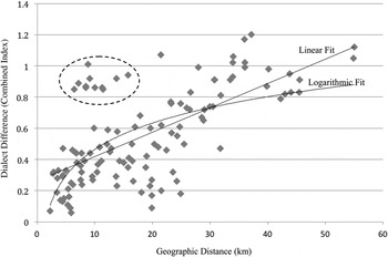
The strongest correlation is found when simple geographic distance is plotted against the Combined Index. Figure 4 shows this very strong and statistically significant correlation. Simple linear geographic distance accounted for a large amount of the dialect differences: 42.8% (r 2 = .428, p ≤ .02, Mantel TestFootnote 6). A logarithmic fit is significant as well (r 2 = .415, p ≤ .02). Note that the logarithmic fit is not quite as strong as the linear fit, and there is no significant difference (p ≤ .18).Footnote 7 In the prior literature, a logarithmic fit (Seguy's Curve) has usually been better than a linear fit. The greater effectiveness of the linear fit for Sui may be due to the small geographic size of the Sui study (cf. Nerbonne & Heeringa's [2007] study of Lower Saxony, Germany). Implications of this result are discussed in the Conclusion section.
Sui geographic distance plotted against dialect difference (Combined Index). Each point in the figure represents the comparison of two locations, for example, the geographic distance between Location A and Location B and the dialect difference between Locations A and B. Linear and logarithmic trend lines are included. The dotted ellipse is discussed in the text.

The Lexical/Phonological Index also produces a significant correlation between geographic distance and dialect difference: r 2 = .120, p ≤ .04. However, note that this correlation is much weaker than the Combined Index result (r 2 = .428). Presumably, this is because any dialectometry study is limited by the particular words in the sample. When the lexical variants are separated out from phonological variants in the calculation of the Lexical/Phonological Index, this may put undue weight on certain lexical variants that happen to occur in a dataset. If, instead, a sample of thousands of words were collected for each location, it is likely that the Phonological/Lexical Index would perform more similarly to the Combined Index. For this Sui study, the Combined Index produces the strongest correlations, and it closely reflects the results of prior work in other societies (16% to 38% correlation). For these reasons, the Combined Index will be used for the remainder of the analysis.
Although most of the data points in Figure 4 lie fairly close to the trend lines, there are some relatively poorly fitted data points. First, there is a clearly isolated cluster of points above the trend lines (marked with a dotted ellipse). These points are all associated with Location N (Yang'an dialect). There is also a cluster of poorly fitted points below the trend lines at around 18 to 25 km, some of which are associated with Location L. Issues related to Locations N and L are discussed in the following section.
Nonetheless, the overall fit is very strong: 42.8% of the data is accounted for by simple geographic distance. In this way, the results for Sui are as strong or stronger than the 16% to 38% range seen in prior work on other languages (Nerbonne, Reference Nerbonne2010). Considering how divergent Sui culture is from the other languages used in past dialectometry work, this result is a bit surprising. Because clan ideology is so important to local Sui sociolinguistics, and because the society covers only a small geographic region, one might suspect that dialectometry would be more difficult to apply in this context. Yet it actually works very well. On the other hand, this result does not hold true when peripheral locations are excluded from the analysis.
An analysis that excludes the four peripheral locations
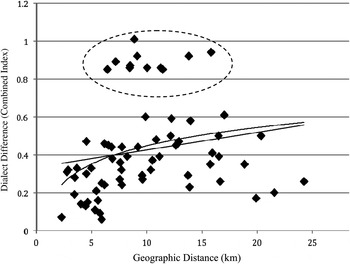
Note from the map in Figure 3 that four locations are relatively distant from the rest: A, B, L, and Q. This is because the present study was patterned on the locations of SDB (1956) and the natural geographic distribution of the Sui population. Because these four data points represent a large amount of the geographic distance in the regressions, it is good statistical practice to check the regression results without these peripheral locations. After removing Locations A, B, L, and Q, the remaining 12 locations have a maximum paired distance of 24 km (the distance from C to P), which is considerably lower than the maximum 55 km in the full dataset (the distance from A to Q). The results are shown in Figure 5, including linear and logarithmic trend lines. The linear fit is very weak and not significant: r 2 = .036, p ≤ .25 (Mantel TestFootnote 8). The logarithmic fit is also very weak and not significant: r 2 = .044, p ≤ .25. Just like Figure 4, Figure 5 has one cluster of data points that are isolated from the rest (dotted ellipse). These data points correspond to pairwise calculations involving Location N, which is the Yang'an dialect region. When Location N is excluded from the analysis, the linear fit is improved but still weak: r 2 = .106, p ≤ .07. The logarithmic fit is similar (r 2 = .107, p ≤ .07). Therefore, even when Yang'an is accounted for, the short-range dataset (24-km range) does not have strong correlations between geographic distance and dialect differences.
Results when the four peripheral locations are excluded (A, B, L, Q).

Sui dialect continuum?
The results also provide insights into Sui dialect regions. Three major Sui dialect regions have been described in prior work (Zhang, Reference Zhang1980). The largest region, the Sandong dialect or “Central Sui,” covers the central part of Sandu County. The Pandong dialect is located to the northwest, and the Yang'an dialect in the west. Castro (Reference Castro2011) suggested a fourth dialect “Southern Sui,” located to the south of those three dialect regions. Speakers generally report a high degree of mutual intelligibility between these dialects, and most of the regional differences in Sui dialects are phonological and lexical, not morphosyntactic. The geographic points in the present study include samples from all four dialect regions.
In both Figure 4 and Figure 5, most of the data points lie fairly close to the linear and logarithmic trend lines. This result suggests that most Sui dialects lie along a dialect continuum, in other words, the dialect differences increase fairly predictably over distance. But the dotted ellipse of data points associated with the Yang'an dialect (Location N) is considerably far from the trend lines. Therefore, the Yang'an dialect is considerably different, despite its relatively close proximity to the central area. This result matches the opinions of Sandong dialect (Central Sui) speakers when asked about the Yang'an dialect, and they have varying opinions about why Yang'an speakers may have developed such a different dialect. The specific social or migratory reasons for this dialect's divergence from the main continuum await a future study.
In addition to the poorly fitted results from Yang'an, another location (Bajie, Location L) is responsible for some of the low scores around 18 to 25 km in Figure 4. Sui informants consider the speech of Location L to be quite similar to that of Location M, which is in the central area. Yet, recalling the map in Figure 3, there is a relatively large distance between L and M. Local informants comment that perhaps the residents of Location L originated farther south around Location M, noting that many residents in these two locations share a common surname, Pan. This might explain why the dialect differences between Location L and other locations are somewhat lower than would be expected by its geographic distance. Even so, Yang'an (Location N) is the only location that produces a sharply isolated group. The other locations are close to a predictable continuum.
Summary
For the full dataset (16 locations with a maximum range of 55 km), the Combined Index provides a very strong, statistically significant correlation with simple geographic distance (42.8%). The amount of variation accounted by simple geographic distance is therefore comparable to (and even slightly better than) the 16% to 38% range expected from Nerbonne (Reference Nerbonne2010). However, unlike Seguy's Curve, the logarithmic fit is slightly weaker than the linear fit, and there is no significant difference. The Lexical/Phonological Index also provides a significant correlation (12%), but it is weaker than the Combined Index.
When the four peripheral locations (A, B, Q, and L) are excluded, the remaining short-range set (24-km range) shows only a very weak, nonsignificant correlation between geographic distance and dialect difference. Even when the divergent Yang'an dialect region (Location N) is excluded from this short-range set, the correlations are weak.
The results also provide dialectometric evidence that most of the locations fall along a relatively smooth, predictable dialect continuum, whereas the Yang'an dialect is more divergent.
“Paddy-adjusted distances”
Geographic distance strongly correlates with Sui dialect differences, but one wonders whether such Euclidean distance measurements appropriately represent the social spaces experienced in Sandu County (cf. Britain, Reference Britain, Chambers, Trudgill and Schilling-Estes2002:604). After all, people rarely travel in simple straight lines from place to place. Prior research in other countries suggests that “travel distance” may be important to consider. In dealing with the fjords of Norway, Gooskens (Reference Gooskens2005) calculated Norwegian dialect distance in terms of travel times along roads. She found that this approach provides a stronger correlation than simple geographic distance does.Footnote 9 Similarly, Buchstaller and Alvanides (Reference Buchstaller and Alvanides2010) showed the effectiveness of calculating distance with respect to “Travel-to-Work-Areas” in northeast England. Trudgill compared sea and land travel distances in Norway (1974). Labov (Reference Labov and Silverstein1974) examined dialect features in terms of Eastern U.S. traffic patterns, finding that the amount of traffic flow correctly accounted for all but one of the variables he tested (Labov, Reference Labov2001:18).
Such approaches do not translate smoothly into Sui culture. First, road travel times and traffic patterns are not as useful because the roads of this region are recently built and do not necessarily reflect travel patterns in earlier times. Moreover, even taking contemporary roads into account, the actual routes taken between individual villages often include a maze of small paths not found on maps or satellite imagery. The first (gravel) road serving this central part of Sandu County was not built until 1959 (Luo, Reference Luo1992:523; Pan, Wang, Luo, & Shi, Reference Pan, Wang, Luo and Shi1984:333–334; Sandu Shuizu Zizhixian Gaikuang, 1986:119), and it was not paved until 2002. (The road runs north-south, passing near Locations E, G, I, J, M, O, and Q.)
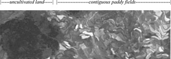
What would be a culturally appropriate Sui equivalent of travel distance? One possibility is to consider the role of rice paddies in Sui social geography. Rice paddy fields are easily visible through publicly available satellite imagery (Google Earth). Availability of roads has changed over time, but rice paddies represent long-term social patterns. In this patriarchal society, paddy fields are passed down through the generations from father to son, so they are a considerably stable element of social geography. Many paddy fields are terraced along hillsides with complex water rights, and so it would require considerable physical (and social) effort to change their locations. Some changes occur over generations, but the paddy fields nonetheless form a clearly visible record of human culture expressed by and constructed in local geography—a meaningful geophysical sign of human culture in the terrain. In many societies, cities are a visible sign of social interaction; for example, Labov (Reference Labov2008) examined nighttime satellite imagery of concentrations of city lights as a representation of social patterns in the U.S. Inland North. In the same way, concentrations of rice paddies represent patterns of social interaction in rural Sui agricultural society. Figure 6 shows an example of a satellite image from Google Earth showing a small portion of the Sui region. Note the paddy fields in contrast with nearby uncultivated land.
Example of satellite imagery of Sandu County: Rice paddy fields in contrast to uncultivated land. Source: Google Earth, ©2011 GeoEye, 2011 Cnes/Spot Image, 2010 Mapabc.

Considering the notion that face-to-face interaction correlates with linguistic variation and change (Bloomfield, Reference Bloomfield1933; Trudgill, Reference Trudgill1986), perhaps rice paddy geography can help provide a deeper understanding of Sui dialects. The assumption is that long-term contact between speakers is greater in areas of contiguous rice paddies than in areas separated by nonarable land. On this basis, a “Paddy-Adjusted Distance” (PAD) was calculated for the present study.
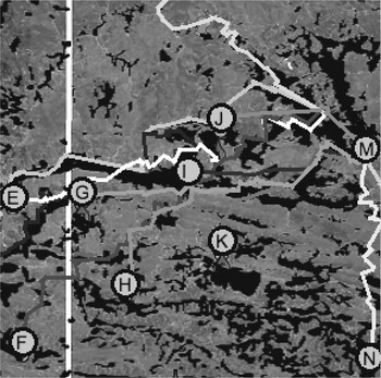
First, rice paddies in the satellite imagery were manually “painted” black with Google Earth's “Insert Polygon” function, using zoomed-in views such as Figure 6. This procedure resulted in a JPEG file with graphical contrasts between rice paddies (black pixels) and uncultivated land (pixels of any other color). Rice paddies were the main focus of this procedure, but villages were also painted black because most Sui villages also represent very long-term settlements. It should also be noted that, due to varying resolution in some of the satellite images, it was not always possible to differentiate rice paddies from other planted fields (which might be less permanent). Nonetheless, this procedure provides a reasonably accurate geographical picture of the long-term patterns of human activity across the region.
A program was then written to calculate a “path of least resistance” between any two points, such as, the route that goes through the most rice paddies and the least uncultivated land (the program was written in Python by Tev'n J. Powers). The program reads each pixel in a JPEG file as either black (rice paddies) or nonblack (uncultivated land), and it calculates the best routes between pairs of locations. We used the program to calculate these routes for all 120 pairwise combinations of the 16 locations, with a scale of 20.7 pixels per kilometer or about 21 “choices” per kilometer. For each pairwise computation between locations, the program outputted the total number of pixels traveled in the chosen path, which is the PAD. Figure 7 shows a sample screenshot of a few of the computed routes. Note that this algorithm could be potentially useful for other dialect geography applications besides rice paddies.
Examples of a few routes calculated by the computer program. The alphabetical letters correspond to the study locations in Figure 3 (the scene was rotated sideways for analysis). The dark patches are rice paddies that have been “painted” black. The vertical white line is just a gridline used for scaling. Source: Google Earth, © 2011 GeoEye, 2011 Cnes/Spot Image, 2010 Mapabc.

Results for PAD
PAD shows a very strong correlation with dialect differences, coming close to covering half of all dialect variation in the study: PAD accounts for 44.4% of the dialect variation (r 2 = .444, p ≤ .02, Mantel) (using the Combined Index). This is better than the 42.8% result for simple geographic distance, although the improvement is not statistically significant (p ≤ .22, Partial Mantel Test). The logarithm of PAD also shows a strong correlation with dialect differences (r 2 = .402, p ≤ .02), but it is not as strong as the linear correlation. Finally, as with simple geographic distance, when the peripheral points are removed from the dataset (A, B, L, Q), the PAD correlation is no longer significant: r 2 = .047, p ≤ .25.
Analysis
The hypothesis stated earlier turns out to be partially false. Overall, dialectometry actually proved quite effective for this small, non-Western, nonindustrialized, clan-oriented, indigenous society. The Sui dialectometry results were consistent with results from other societies in the sense that geographic distance was strongly correlated with dialect differences. Simple geographic distance accounted for 42.8% of the dialect variation. Using the alternate distance measure, PAD, the correlation was slightly stronger (44.4%), approaching a level of accuracy where dialectometry could account for nearly one-half of all dialect variation in the region.
On the other hand, the correlations were significant only when the full dataset was used (55-km range). The correlations were weak and nonsignificant in the short-range set where peripheral locations were excluded (24-km range). In addition, the logarithmic relationship (Seguy's Curve) was not significantly better than a linear fit in either the full dataset or the short-range dataset. Moreover, all of the results must be tempered with recognition of the actual complexity of dialect contact in Sui villages; dialectometry only makes use of a single score for each location, but many different dialects are spoken in any given Sui village because of in-marriage.
The Sui results are therefore consistent with Nerbonne and Kleiweg's (Reference Nerbonne and Kleiweg2007) Fundamental Dialectological Postulate to a large degree. At the same time, the results can only be fully meaningful when complemented by a localized understanding of the Sui experience of place. A purely “mechanical” analysis of the Sui dialectometry results would give an incomplete picture because it would lack the “local knowledge that motivates and explains the behavior of a particular group” (Johnstone, 2004:76; see also Eckert, Reference Eckert and Fought2004; Hill, Reference Hill and Terrell2001). A deeper understanding of the results can be achieved by examining two issues more carefully: exogamy (the question of “one culture fits all”) and small-scale versus large-scale human interactions (the question of “one size fits all”).
Exogamy (one culture fits all?)
As Bucholtz (Reference Bucholtz2003:403) noted, it is important to bring more diverse communities into the study of language and gender. Sui marriage practices pose challenges for straightforward applications of dialect geography and dialectometry. Because almost all adult Sui women in any village have left their original home villages and in-migrated to their husbands’ villages, women have a key role in Sui contact sociolinguistics. This aspect of Sui society was unfortunately opaque to SDB (1956), which primarily focused on male speakers.
Dialect geography, by its very nature, runs the risk of marginalizing the sociolinguistic importance of Sui women, thereby misreading the social meaning of place in Sui society as a whole. In-married Sui women have a strong sense of place-identity with their clans of origin and loyalty to their original clan dialects, despite daily contact with the dominant dialect of the husband and local villagers (Stanford, Reference Stanford2008a, Reference Stanford2008b, Reference Stanford2009a, Reference Stanford, Stanford and Preston2009b). The role of women and children should be carefully considered when conducting dialect geography of patriarchal exogamous societies, lest their important sociolinguistic roles be overlooked. As outlined in the following, it is very likely that women are at the forefront of Sui dialect contact, variation, and change.
Although many Sui people seasonally migrate to Chinese-speaking regions of the country for labor opportunities, the most intense linguistic contact within Sui society involves the in-migration of women from their home village to the husband's village. This results in daily contact within villages and within households, and it is the most likely cause of any contact-related Sui language change. In addition, because Sui women are traditionally more responsible for child-rearing than men are, the women have a greater potential influence on each successive generation. Stanford (Reference Stanford2008b) found that Sui children quickly acquire the patrilect, that is, the dialect of the father and other locals. Very young children exhibit some matrilectal features, but by age 7 to 9 years, they have acquired the patrilect to a high degree, and they are ridiculed if they use any matrilectal features. Older children and teenagers are almost fully patrilectal, and adults are always patrilectal. Speakers carefully maintain these clan dialects in spite of daily contact within the village and within households.
Although these dialect features appear to be stable across generations, it is reasonable to suppose that very long-term patterns of leveling or diffusion could occur, especially in central regions. Stanford (Reference Stanford2011) confirmed the stability of the dialect distinctions over 50 years, so any change must be very slow. Yet a set of geographically centralized patterns observed in lexical tone and first singular suggest the possibility of slow, long-term leveling/diffusion (Stanford, Reference Stanford2011). If and when such contact-induced change occurs over generations, it is very likely attributable to the role of in-marrying women.
Dialect geography and dialectometry only represent the dominant dialect of each location. A balanced approach should be sensitive to the analytical conundrum inherent to any such study of a patrilocal exogamous society, recognizing the role of women's speech in language variation and change, as well as their role in influencing children's speech (cf. Britain, Reference Britain, Chambers, Trudgill and Schilling-Estes2002:618–619; Stanford, Reference Stanford2008b).
Small societies (one size fits all?)
The second issue to consider involves geographic size, specifically the mathematical fit of the regressions in Figures 4 and 5. In the full dataset (55 km), the results reveal a very strong correlation between geographic distance and dialect difference (Figure 4). However, in the short-range dataset (24 km), the correlation is weak and nonsignificant (Figure 5). Dialectometry results always have a considerable amount of variance due to human individuality and various uncontrolled sociohistorical factors, and so a larger population size/sample size helps to clarify the overall pattern (Figure 1). Moreover, it is a well-known mathematical fact that distant data points contribute more to the strength of a regression than nearer points do; small-range datasets have a narrower spread of x-axis values available to contribute to the fit, and they may have fewer data points overall. Nonetheless, such effects are more “disruptive” to the results in studies of small-scale societies than large-scale societies. Dialectometry studies across large societies have the advantage of a larger geographic spread.
In addition, the sublinear curve (Seguy's Curve) attested in prior work is not better than a simple linear fit in this Sui study. The logarithmic correlation is weaker than the linear correlation, and there is no significant difference between the two. On one hand, this result is not surprising because it matches another study of a relatively small region: Nerbonne and Heeringa's (Reference Nerbonne, Heeringa, Featherston and Sternefeld2007) study of a small region, Lower Saxony, Germany, with a maximum distance of 140 km. Because there was not enough geographic distance involved, the logarithmic pattern did not emerge as being stronger than a linear fit. But should we assume that these patterns cannot be “compressed” to fit smaller societies? After all, other mathematical patterns can retain their shape on wildly different scales.
In the natural world, a pattern is sometimes observed on very different levels of scale. As seen in Figures 8a and 8b, the elegant spiral shape of a nautilus shell shares many of the geometric features of the unimaginably larger spiral of a galaxy. Hurricanes share this shape as well. Similar underlying mathematical principles are operating on different levels of scale to produce those familiar forms of logarithmic spiral geometry in nature (Darling, Reference Darling2004:188–189; Livio, Reference Livio2002).
A. Nautilus shell. Source: © Hot99 | Dreamstime.com. B. Spiral galaxy. Credit: NASA, ESA, and the Hubble Heritage (STScI/AURA)-ESA/Hubble Collaboration. Acknowledgment: R. Chandar (University of Toledo) and J. Miller (University of Michigan).
It is therefore plausible that principles of language and physical distance can also operate on different levels of scale. This Sui project is far smaller in geographic range than studies like ANAE or the dialectometry studies reported in Nerbonne (Reference Nerbonne2010) (reprinted in Figure 1), yet comparable in terms of accounting for variation across the greater part of a whole society. Purely from a mathematical point of view, there is nothing to prevent the dialectometric patterns of large societies from appearing in smaller societies as well. Dialectometry studies do not involve the specific mathematical properties seen in Figures 8a and 8b (logarithmic spiral), but they do involve other mathematical properties, namely, Seguy's Curve. Despite the mathematical plausibility of such patterns at a small scale, it appears that the patterns of dialectometry do not simply “compress” as the size becomes smaller.
For galaxies and nautilus shells, mathematical patterns can simply be compressed or expanded to fit vastly different scales. Apparently, human dialect behavior cannot. The human interactions that underlie dialectometric patterns are not so compressible. In a small-distance study in the Netherlands (140-km range), Nerbonne and Heeringa (Reference Nerbonne, Heeringa, Featherston and Sternefeld2007) found that a logarithmic fit (i.e., Seguy's Curve) was not better than a linear fit: “In this case, the linear model is slightly better than the logarithmic model, but there is no significant difference between the two” (p. 289). In addition, note that it is not simply a matter of the number of data points; Nerbonne and Heeringa's (Reference Nerbonne, Heeringa, Featherston and Sternefeld2007:286, 290) study actually had a very robust number of data points (1,326 pairs of dialect difference/geographic distance) covering that small range of 140 km. Nerbonne and Heeringa interpreted the relative lack of strength of the logarithmic fit in that particular study as being due to the small distances involved: “Since linguistic distance tends to rise to a ceiling when large enough areas are examined, the logarithmic model functions in general better” (p. 289).
Another useful perspective involves considering the “building blocks” of the different patterns. For the geometric patterns of galaxies, the basic building blocks are stars, which are huge in size. For nautilus shells, the basic building blocks are molecules of calcium carbonate, which are tiny in size. The same logarithmic spiral geometry can appear in both cases because the building blocks themselves differ vastly in size. By contrast, for human dialect geography, the basic building blocks are the same in both large and small communities: humans and their personal interactions. For this reason, the mathematical patterns of dialectometry in large communities are not necessarily compressible to fit smaller communities.
In terms of dialect geography, then, what are the key differences between large communities and small communities? One difference is that smaller regions have a greater likelihood of kinship relationships, which can affect dialect features. More generally, frequency of human contact is a major difference between large and small communities. Smaller overall scale naturally means that there is less overall physical distance between regions and therefore less overall physical separation of speakers. In this sense, it is a matter of physical limitations of humans, and so this might be generalizable in broad terms of distance and traveling effort.
All things being equal in terms of transportation and other factors, there may be a low-end range where social interactions are frequent enough that physical distance is usually not important enough to correlate with dialect differences. Perhaps an hour of modestly paced walking or a similar distance on a farmer's horse-cart are good estimates of the range where geographic distance typically begins to have a significant correlation with dialect—at least in societies whose modern dialect patterns continue to reflect preindustrial settlements (e.g., Labov, Reference Labov2010:219). Suppose this distance is roughly 5 km.
It may then be possible to speculate that there is a “lower limit,” a minimal distance typically required for dialect geography to be relevant, all things being equal with respect to other factors. Owing to differences in age, ethnicity, class, gender, social identity, and such, dialect variation can occur within a single city block or within a single house. Political boundaries, terrain, transportation, and many other factors can be significant as well (e.g., Chambers, Reference Chambers1994). But all things being equal, suppose that the smallest distance for dialect geography to be relevant in a given community might be about 5 km, given the results in Figure 4 and Figure 1 and the effort required for traveling in preindustrial societies. This estimate could be tested and refined in further work. As for Seguy's Curve, it appears that this familiar logarithmic relationship is not better than a linear fit in ranges below approximately 100 km (Nerbonne & Heeringa, Reference Nerbonne, Heeringa, Featherston and Sternefeld2007:289–290) (Figure 4), regardless of whether or not the study encompasses the entire society.
CONCLUSION
For the Sui people, place is constructed through a complex interplay of clan loyalties and dialect contrasts between local villagers and in-marrying women. Yet simple physical proximity is also a major factor as language is constructed through face-to-face interactions in physical contexts; the dialectometry results show a very strong correlation between physical distance and dialect differences. Even so, the patterns of dialectometry are not simply compressible. There is a difference between large and small societies; it is not simply a matter of reducing the dialectological patterns proportionally to fit a smaller society. Instead, the issue of geographic size appears to be related to fundamental distance relationships in human interactions.
Hill's (Reference Hill and Terrell2001) notion of “anthropological dialectology” and Friedrich's (Reference Friedrich and Edmonson1984) “pueblo dialectology” highlighted the need for sensitivity to the cultural particulars of small rural indigenous populations. The present study concurs, noting that dialectometry does not address key facts about Sui clan ideology and dialect complexity within villages. But many of the broad generalizable results of dialectometry have also proved meaningful in this study. Both sides of the analytical coin are valuable.