1 Introduction
Consider a contact line formed by a pure liquid, an inert gas such as air and a flat rigid substrate. It is an object inherently associated with singularities, appearing when it is modelled in the framework of standard thermo-hydrodynamics. These singularities can be motion related (Huh & Scriven Reference Huh and Scriven1971; de Gennes Reference de Gennes1985) and/or, for volatile liquids, phase-change related (see e.g. Deegan et al. Reference Deegan, Bakajin, Dupont, Huber, Nagel and Witten1997; Rednikov & Colinet Reference Rednikov and Colinet2013). The flux divergence is different for evaporation from a fixed-temperature superheated substrate into a pure-vapour atmosphere (see e.g. the discussion in Rednikov & Colinet Reference Rednikov and Colinet2013), and for (isothermal) diffusion-limited evaporation into an inert gas (Deegan et al. Reference Deegan, Bakajin, Dupont, Huber, Nagel and Witten1997). It is non-integrable in the former case, but integrable for the latter. Nonetheless, in spite of such integrability, there still remains a non-integrable singularity as far as the evaporation-induced flow in the liquid is concerned. Namely, the total viscous dissipation diverges, the divergence being even stronger than the classical logarithmic one prevailing for a moving contact line (de Gennes Reference de Gennes1985; Rednikov & Colinet Reference Rednikov and Colinet2013). It is noteworthy that temperature variations due to the latent heat of phase change and to a finite thermal conductivity of the substrate do not in fact lead to a removal of the flux divergence at the contact line, as can be verified in the diffusion-limited case with the help of a local solution obtained by Ristenpart et al. (Reference Ristenpart, Kim, Domingues, Wan and Stone2007).
The resolution of all these singularities is generally achieved by incorporating various microphysics effects typically beyond standard thermo-hydrodynamics, such as e.g. the (Derjaguin) disjoining pressure and related precursor films (de Gennes Reference de Gennes1985; Derjaguin, Churaev & Muller Reference Derjaguin, Churaev and Muller1987; Bonn et al. Reference Bonn, Eggers, Indekeu, Meunier and Rolley2009), the Navier slip (Huh & Scriven Reference Huh and Scriven1971; Bonn et al. Reference Bonn, Eggers, Indekeu, Meunier and Rolley2009), diffuse interfaces (Pismen & Pomeau Reference Pismen and Pomeau2000; Sibley et al. Reference Sibley, Nold, Savva and Kalliadasis2013) and the kinetic resistance to phase change associated with departure from the local phase equilibrium at the liquid–gas interface (Burelbach, Bankoff & Davis Reference Burelbach, Bankoff and Davis1988).
Whatever the mechanism(s) eventually regularising the singularities at the microscales, the local flux and the associated flow in the liquid still appear to considerably intensify towards the contact line at the macroscales. This intense dynamics is at the origin of the evaporation-induced contact angles established in some ‘microregion’ of the contact line and perceived as apparent contact angles at larger scales. Thus, in particular, even if the liquid perfectly wets the substrate and the contact line is at rest, finite evaporation-induced angles are expected. In the partial-wetting case, Young’s angle is modified by evaporation in the sense of an increase of the apparent contact angles. Conversely, condensation is expected to make them decrease with respect to their equilibrium value (see e.g. Rednikov & Colinet Reference Rednikov and Colinet2013). Contact-line motion can lead to further modifications of the apparent contact angles in accordance with the Cox–Voinov relation (Voinov Reference Voinov1976; de Gennes Reference de Gennes1985; Cox Reference Cox1986; Bonn et al. Reference Bonn, Eggers, Indekeu, Meunier and Rolley2009; Rednikov & Colinet Reference Rednikov and Colinet2013; Snoeijer & Andreotti Reference Snoeijer and Andreotti2013).
Such evaporation-induced angles have been obtained both in experiments and in theoretical studies, irrespective of whether evaporation is into a pure-vapour atmosphere (the substrate being superheated) or into an inert gas (Potash & Wayner Reference Potash and Wayner1972; Moosman & Homsy Reference Moosman and Homsy1980; Stephan & Busse Reference Stephan and Busse1992; DasGupta, Kim & Wayner Reference DasGupta, Kim and Wayner1994; Hocking Reference Hocking1995; Morris Reference Morris2001; Ajaev Reference Ajaev2005; Guéna, Poulard & Cazabat Reference Guéna, Poulard and Cazabat2007; Berteloot et al. Reference Berteloot, Pham, Daerr, Lequeux and Limat2008; Rednikov, Rossomme & Colinet Reference Rednikov, Rossomme and Colinet2009; Ajaev, Gambaryan-Roisman & Stephan Reference Ajaev, Gambaryan-Roisman and Stephan2010; Eggers & Pismen Reference Eggers and Pismen2010; Pham et al. Reference Pham, Berteloot, Lequeux and Limat2010; Colinet & Rednikov Reference Colinet and Rednikov2011; Doumenc & Guerrier Reference Doumenc and Guerrier2011; Janeček & Nikolayev Reference Janeček and Nikolayev2012; Raj et al. Reference Raj, Kunkelmann, Stephan, Plawsky and Kim2012; Doumenc & Guerrier Reference Doumenc and Guerrier2013; Janeček et al. Reference Janeček, Andreotti, Pražák, Bárta and Nikolayev2013; Janeček & Nikolayev Reference Janeček and Nikolayev2013; Rednikov & Colinet Reference Rednikov and Colinet2013; Oliver et al. Reference Oliver, Whiteley, Saxton, Vella, Zubkov and King2015; Saxton et al. Reference Saxton, Whiteley, Vella and Oliver2016; Savva, Rednikov & Colinet Reference Savva, Rednikov and Colinet2017).
A full account of microphysics in the framework of a macroscopic problem leads in fact to highly disparate length scales within the computation domain. A separate consideration of the microregion, where the contact-line singularities are resolved and apparent contact angles are established, can thus be rather advantageous. Furthermore, the associated decoupling proves indeed to be possible to leading order (in the length scale ratio), only maybe up to one or a few input parameter(s) determined by the macroscopic set-up. Thus, a microregion problem ends up by being well defined on its own. It naturally possesses a higher degree of universality than any given macroscopic configuration. A vast literature is already available containing considerations of the microregion problem in its own right both in the pure-vapour case (Potash & Wayner Reference Potash and Wayner1972; Stephan & Busse Reference Stephan and Busse1992; DasGupta et al. Reference DasGupta, Kim and Wayner1994; Morris Reference Morris2001; Rednikov et al. Reference Rednikov, Rossomme and Colinet2009; Colinet & Rednikov Reference Colinet and Rednikov2011; Janeček & Nikolayev Reference Janeček and Nikolayev2012; Janeček et al. Reference Janeček, Andreotti, Pražák, Bárta and Nikolayev2013; Janeček & Nikolayev Reference Janeček and Nikolayev2013; Rednikov & Colinet Reference Rednikov and Colinet2013; Oliver et al. Reference Oliver, Whiteley, Saxton, Vella, Zubkov and King2015; Savva et al. Reference Savva, Rednikov and Colinet2017) and in the inert-gas one (Berteloot et al. Reference Berteloot, Pham, Daerr, Lequeux and Limat2008; Pham et al. Reference Pham, Berteloot, Lequeux and Limat2010; Colinet & Rednikov Reference Colinet and Rednikov2011; Morris Reference Morris2014; Saxton et al. Reference Saxton, Whiteley, Vella and Oliver2016).
It is precisely a microregion problem that we are concerned with in the present paper. We consider it for a volatile liquid in the presence of vapour exchange with an inert-gas atmosphere. The goal is twofold. First, it is to demonstrate that no microphysics effect beyond standard thermo-hydrodynamics among those listed in the second paragraph of this section is actually indispensable here for the contact-line singularity resolution. They can rather be resolved in the framework of standard thermo-hydrodynamics solely thanks to the Kelvin effect appropriately adjusting the local phase-change rates. (The very idea that a contact line can advance/recede by condensation/evaporation is a long-standing one (cf. Pomeau Reference Pomeau2011, and references therein). However, the contact-line velocity and the local phase-change rates are generally independent physical factors, and it is not a priori clear how their desired mutual adjustment can be realised unless there exists a mechanism such as the Kelvin effect considered here.) Note that the absence of those microphysics effects does not compromise the existence of a microregion and the well posedness of the corresponding problem given that the Kelvin effect is typically essential only at sufficiently small lengths. It is worth emphasising that we here seek to show that such regularisation can be realised for both finite Young’s angle (partial wetting) and a zero one (perfect wetting), for advancing, immobile and receding contact lines, as well as for global evaporation (undersaturated atmosphere), and global phase equilibrium (saturated atmosphere), also touching upon the case of global condensation (oversaturated atmosphere). The second part of the scope concerning calculation of the corresponding evaporation-induced and motion-modified apparent contact angles within such a Kelvin-only paradigm comes essentially as a by-product of the realisation of the first part.
The present paper does not study in detail whether the disjoining pressure (or any other microphysics effect) can really be disregarded in regard to the Kelvin effect from a practical point of view, a legitimate question given that all these effects act at quite small scales. Our goal here is rather to show the new, a priori not evident and conceptually important fact that the Kelvin effect could handle all singularities alone, in the case of diffusion-limited phase exchange. That is why we proceed right away from a ‘minimalist’ formulation, with no microphysics effects incorporated whatsoever. Interestingly enough, the answer to the opposite question of whether this time the disjoining pressure could handle it all alone in the same sense (including a possibly evaporative environment, diffusion-limited in particular, and not just contact-line motion) is not quite evident either, for the models used by Eggers & Pismen (Reference Eggers and Pismen2010), Doumenc & Guerrier (Reference Doumenc and Guerrier2011), Morris (Reference Morris2014) inherently require both the disjoining pressure and the Kelvin effect. Let us limit ourselves here to mentioning that a rigorous positive answer to this latter question can be obtained in the framework of a de-Gennes-like approach (Colinet & Rednikov Reference Colinet and Rednikov2011).
In the case of a pure-vapour atmosphere, a counterpart of the present Kelvin-only program was attempted on heuristic grounds by Wayner (Reference Wayner1993) and rigorously realised by Rednikov & Colinet (Reference Rednikov and Colinet2013). The study by Rednikov & Colinet (Reference Rednikov and Colinet2013) provides a more detailed preamble to the issue of contact-line singularities and treats two particular benchmark cases (immobile contact line with evaporation and an advancing contact line in a saturated atmosphere) setting forth an example to follow here. Other authors, still in the pure-vapour case, have also come to similar developments (Janeček & Nikolayev Reference Janeček and Nikolayev2012; Janeček et al. Reference Janeček, Andreotti, Pražák, Bárta and Nikolayev2013). Strictly speaking, other than inspirationally, the Kelvin-only resolution of contact-line singularities in the pure-vapour case does not yet mean that the same is equally possible for diffusion-limited vapour exchange with an inert-gas atmosphere. Physically and mathematically, these are two distinct problems (e.g. the presence of non-local operators in the film equation for the latter but not for the former), as it will occasionally be pointed out in what follows.
Part of the present Kelvin-only program, already for the case of the diffusion-limited evaporation we are concerned with here, has in fact been realised in a recent study by Janeček et al. (Reference Janeček, Doumenc, Guerrier and Nikolayev2015), albeit within a limited scope. Namely, the Kelvin-only microregion problem was resolved only in the case of a saturated atmosphere, hence there were a priori no evaporative singularities or evaporation-induced contact angles. Besides, the study was limited to moving contact lines with finite Young’s angles (partial wetting). The present study will show that the Kelvin effect can also take care of phase-change-related singularities, occurring in under- or over-saturated atmospheres, both in their pure form and in combination with contact-line motion. The evaporation-induced contact angles and phase-change-related modifications of Young’s angle will be calculated. Furthermore, the case of perfect wetting (zero Young’s angles) will now also form part of the analysis throughout.
Finally, let us mention that the present study is developed within the same general theoretical framework as the previously cited studies, here most relevantly those by Eggers & Pismen (Reference Eggers and Pismen2010), Colinet & Rednikov (Reference Colinet and Rednikov2011), Morris (Reference Morris2014), Janeček et al. (Reference Janeček, Doumenc, Guerrier and Nikolayev2015), Saxton et al. (Reference Saxton, Whiteley, Vella and Oliver2016). Namely, we use the lubrication approximation in the liquid, in particular implying small film slopes and contact angles. The gas medium is dynamically passive. However, the latter does not necessarily imply a fully one-sided model as it does in the pure-vapour case considered elsewhere, vapour diffusion being a paramount effect here. The vapour is assumed to be dilute and transported through the gas phase by pure diffusion. This process is treated in the quasi-steady approximation and the boundary conditions at the film (notably, the vapour concentration attaining its saturation value) are transposed to the flat substrate in view of the assumed film thinness. The problem is assumed to be isothermal.
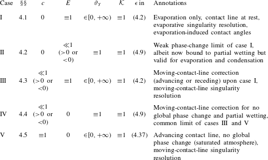
The paper is organised as follows. In § 2, the formulation of the ‘Kelvin-only’ microregion problem is provided in dimensional and then in dimensionless form. The problem is solved for five emblematic, benchmark cases, whose preliminary overview is given below in this section and then in § 3. (For instance, it is these cases that will exhaust a possible asymptotic analysis of volatile sessile drop dynamics of the style of Saxton et al. (Reference Saxton, Whiteley, Vella and Oliver2016) and Savva et al. (Reference Savva, Rednikov and Colinet2017) as far as the microregion part of the problem is concerned.) These cases are analysed one by one in § 4 in the corresponding five subsections (§§ 4.1–4.5) and conclusions are summarised in § 5. Certain details are relegated to appendices A–C.
In § 4.1 (case I), a Kelvin-only resolution of the purely evaporative singularity for a contact line at rest is studied and evaporation-induced contact angles are calculated. Young’s angle is allowed to be either zero (perfect wetting) or finite (partial wetting). In a sense, this part is a Kelvin-only counterpart of the recent study by Morris (Reference Morris2014), also extended to include partial wetting.
In § 4.2 (case II), the same situation is considered by perturbations when phase-change-induced contributions into the contact angle are small relative to a finite Young’s angle. In this latter case, in return, the global phase change is allowed to be either evaporation or condensation, whereas it is only evaporation that is considered for case I in § 4.1. (In our Kelvin-determined microregion, due to the modification of the saturation vapour pressure by the Kelvin effect, the direction of the phase change may in principle locally not coincide with the macroscopically imposed ‘global’ one that takes place at the outer (macroscopic) edge of the microregion under the conditions when the Kelvin effect already becomes negligible.)
In § 4.3 (case III), we take up the case of § 4.1, but now allow the contact line to move (either advance or recede), which effect is treated as perturbation. In particular, this permits a first test of the Kelvin-only resolution of the moving-contact-line singularity.
In § 4.4 (case IV), the singularity of a moving (advancing or receding) contact line is treated in a pure form, in the absence of global phase change (e.g. saturated ambient atmosphere). However, the contact-line motion and motion-induced contact angles are still treated as perturbations on the background of a finite Young’s angle. Note that the recent study by Janeček et al. (Reference Janeček, Doumenc, Guerrier and Nikolayev2015) is bound to case IV in our terms. (Their consideration is however more general in another respect: they additionally incorporate the effect of the kinetic resistance to phase change into their model, not accounted for in our minimalist approach here.)
In § 4.5 (case V), still in the absence of global phase change, the contact-line motion is at last allowed to be a finite and dominant effect, the zero Young’s angle now becoming a fully accessible particular case. In return, only advancing contact lines are allowed in this part of the analysis, carried out in the spirit of Hervet & de Gennes (Reference Hervet and de Gennes1984).
Thus, the effects of advancing contact lines or global evaporation are here generally allowed to be order-unity factors, including the case of perfect wetting. In contrast, we limit ourselves to just perturbative treatments of receding contact lines (dewetting) and global condensation at a finite Young’s angle, leaving beyond the scope the question of critical speeds for a contact line to be no longer sustainable (cf. Eggers Reference Eggers2004).
Appendix A is concerned with the validity criteria for the isothermal treatment of the problem. Estimations of certain results for different liquids are given in appendix B. Appendix C provides further details of coordinate expansions for the film thickness and the vapour concentration at the outer (macroscopic) edge of the microregion.
2 Formulation
2.1 Configuration
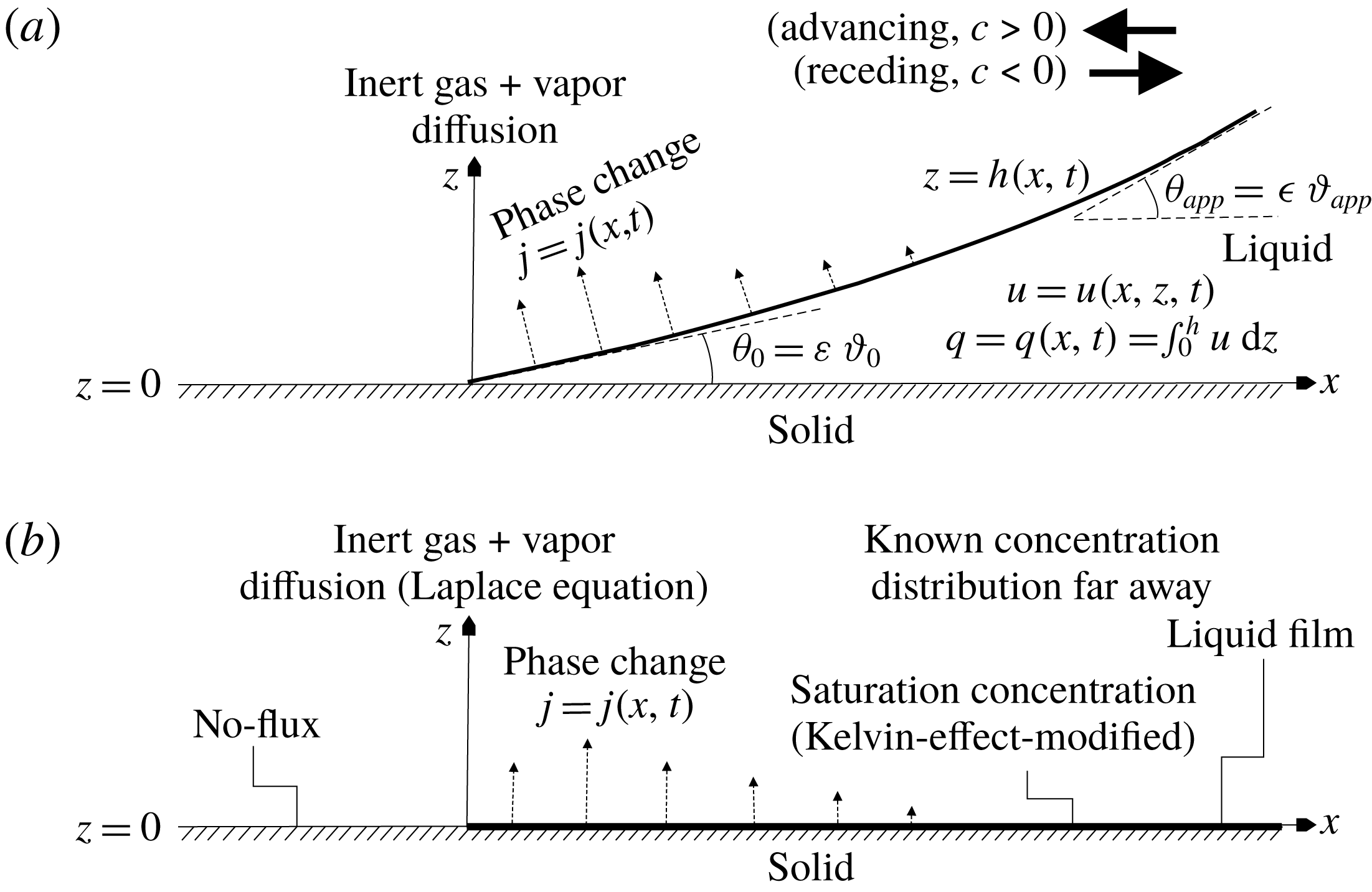
We consider a distinguished small vicinity (microregion) of a contact line formed by a volatile liquid film situated on a flat rigid substrate in an inert-gas atmosphere (see figure 1). The problem pertains to a planar geometry. The microscales characterising such a microregion are to be determined. The film is assumed to start abruptly on a flat rigid substrate with a contact angle
 $\unicode[STIX]{x1D703}_{Y}$
. It is interpreted as Young’s angle and presumed known in the present analysis. (We note that elsewhere (Rednikov & Colinet Reference Rednikov and Colinet2013) we used the notation ‘
 $\unicode[STIX]{x1D703}_{0}$
’ in lieu of ‘
 $\unicode[STIX]{x1D703}_{Y}$
’.) For
 $\unicode[STIX]{x1D703}_{Y}>0$
, we have partial wetting. Perfect wetting will correspond to an important particular case
 $\unicode[STIX]{x1D703}_{Y}=0$
in this scheme. Far away from the microregion (to the right in figure 1), an apparent contact angle
 $\unicode[STIX]{x1D703}_{app}$
is generated. It may be of a different nature in different parts of the present study.
Sketch of the microregion: thin liquid film (a) considered to be of negligible thickness within the diffusion problem in the gas (b). Young’s angle
 $\unicode[STIX]{x1D703}_{Y}=\unicode[STIX]{x1D716}\,\unicode[STIX]{x1D717}_{Y}$
is given (
 $\unicode[STIX]{x1D703}_{Y}=0$
for perfect wetting), while the apparent angle
 $\unicode[STIX]{x1D703}_{app}=\unicode[STIX]{x1D716}\,\unicode[STIX]{x1D717}_{app}$
is to be determined,
 $\unicode[STIX]{x1D716}\ll 1$
is an appropriate small parameter, and generally
 $\unicode[STIX]{x1D717}_{Y}=O(1)$
and
 $\unicode[STIX]{x1D717}_{app}=O(1)$
. In different contexts studied here,
 $\unicode[STIX]{x1D703}_{app}$
can be just
 $\unicode[STIX]{x1D703}_{mic}$
,
 $\unicode[STIX]{x1D703}_{evap}$
or a Cox–Voinov value of the apparent contact angle. All the angles
 $\unicode[STIX]{x1D703}$
are expressed in radians, unless stated otherwise.

The angles and film slopes are assumed sufficiently small,
 $O(\unicode[STIX]{x1D716})$
, where
 $\unicode[STIX]{x1D716}\ll 1$
. The appropriate form of the dimensionless number
 $\unicode[STIX]{x1D716}$
, composed of the physical characteristics of the system, is to be determined depending on the case at hand.
2.2 Equations and boundary conditions for the film thickness
Let
 $h^{\ast }(x^{\ast },t^{\ast })$
be the film thickness,
 $t^{\ast }$
the time,
 $x^{\ast }$
and
 $z^{\ast }$
the Cartesian coordinates,
 $u^{\ast }(x^{\ast },z^{\ast },t^{\ast })$
the longitudinal velocity component,
 $q^{\ast }(x^{\ast },t^{\ast })$
the volume flux,
 $p^{\ast }(x^{\ast },t^{\ast })$
the pressure in the film and
 $j^{\ast }(x^{\ast },t^{\ast })$
(
 $\text{kg}~\text{m}^{-2}~\text{s}^{-1}$
) the local phase-change rate (density) (
 $j^{\ast }>0$
for evaporation and
 $j^{\ast }<0$
for condensation), cf. figure 1. The lubrication approximation yields
 $u^{\ast }=\unicode[STIX]{x1D707}_{l}^{\ast -1}\unicode[STIX]{x2202}p^{\ast }/\unicode[STIX]{x2202}x^{\ast }\,(z^{\ast 2}/2-h^{\ast }z^{\ast })$
, which corresponds to a stress-free surface and a no-slip bottom of the liquid layer, and
 $$\begin{eqnarray}\frac{\unicode[STIX]{x2202}h^{\ast }}{\unicode[STIX]{x2202}t^{\ast }}+\frac{\unicode[STIX]{x2202}q^{\ast }}{\unicode[STIX]{x2202}x^{\ast }}+\frac{j^{\ast }}{\unicode[STIX]{x1D70C}_{l}^{\ast }}=0,\quad q^{\ast }=-\frac{h^{\ast 3}}{3\unicode[STIX]{x1D707}_{l}^{\ast }}\frac{\unicode[STIX]{x2202}p^{\ast }}{\unicode[STIX]{x2202}x^{\ast }},\quad p^{\ast }=p_{0}^{\ast }-\unicode[STIX]{x1D6FE}^{\ast }\frac{\unicode[STIX]{x2202}^{2}h^{\ast }}{\unicode[STIX]{x2202}x^{\ast 2}},\quad \unicode[STIX]{x1D70E}_{\unicode[STIX]{x1D70F}}^{\ast }=-h^{\ast }\frac{\unicode[STIX]{x2202}p^{\ast }}{\unicode[STIX]{x2202}x^{\ast }}.\end{eqnarray}$$
Here
 $\unicode[STIX]{x1D70C}_{l}^{\ast }$
and
 $\unicode[STIX]{x1D707}_{l}^{\ast }$
are the liquid density and dynamic viscosity,
 $p_{0}^{\ast }$
the ambient gas pressure,
 $\unicode[STIX]{x1D6FE}^{\ast }$
the liquid–gas interfacial tension,
 $\unicode[STIX]{x1D70E}_{\unicode[STIX]{x1D70F}}^{\ast }=\unicode[STIX]{x1D707}_{l}^{\ast }\unicode[STIX]{x2202}u^{\ast }/\unicode[STIX]{x2202}z^{\ast }|_{z^{\ast }=0}$
is the viscous shear stress exerted upon the substrate and
 $p^{\ast }$
involves only the Laplace pressure (gravity is negligible at the microscale, whereas the disjoining pressure is ignored as intended).
For a moving contact-line problem (velocity
 $c^{\ast }$
), we will have quasi-stationary microregion profiles with
 $\unicode[STIX]{x2202}h^{\ast }/\unicode[STIX]{x2202}t^{\ast }=c^{\ast }\,\unicode[STIX]{x2202}h^{\ast }/\unicode[STIX]{x2202}x^{\ast }$
in (2.1a
). In particular, we shall consider immobile (
 $c^{\ast }=0$
), advancing (
 $c^{\ast }>0$
) and receding (
 $c^{\ast }<0$
) contact lines, cf. figure 1. The contact-line velocity is dictated by the overall macroscopic situation. Within a microregion problem such as ours, it is just a given input parameter.
In accordance with the stated configuration, the boundary conditions at the tip of the film (
 $x^{\ast }=0$
) are
 $h^{\ast }=0$
and
 $\text{d}h^{\ast }/\text{d}x^{\ast }=\unicode[STIX]{x1D703}_{Y}$
(
 $\unicode[STIX]{x1D703}_{Y}=0$
in the perfect-wetting case). The bare substrate is located at
 $x^{\ast }<0$
, and the film at
 $x^{\ast }>0$
, cf. figure 1. Clearly, no solution with such boundary conditions is possible for a moving contact line in the case of a non-volatile liquid (
 $j^{\ast }\equiv 0$
) within standard thermo-hydrodynamics due to classical contact-line singularities (e.g. Huh & Scriven Reference Huh and Scriven1971; de Gennes Reference de Gennes1985; Rednikov & Colinet Reference Rednikov and Colinet2013). It may here only be possible for volatile liquids with an appropriate form of
 $j^{\ast }$
, cf. Rednikov & Colinet (Reference Rednikov and Colinet2013). In the present paper, we show that diffusion-limited exchange with an inert-gas atmosphere does lead to such an appropriate form of
 $j^{\ast }$
once the Kelvin effect is taken into account.
At the scales of the microregion, the macroscopic part of the liquid is formally located at
 $x^{\ast }\rightarrow +\infty$
and the macroscopic curvature is negligible. Thus, the boundary condition posed as
 $x^{\ast }\rightarrow +\infty$
is here
 $\text{d}^{2}h^{\ast }/\text{d}x^{\ast 2}\rightarrow 0$
(while
 $h^{\ast }\rightarrow +\infty$
). This is compatible with the possibility of defining an apparent contact angle
 $\unicode[STIX]{x1D703}_{app}$
at the outer edge of the microregion, cf. figure 1.
2.3 Vapour diffusion and the Kelvin effect
A closure to the formulation is provided by the problem of vapour transfer in the gas phase (air), yielding in particular an expression for
 $j^{\ast }$
. It is assumed that the vapour is dilute (negligible Stefan flow) and its transfer is accomplished quasi-steadily by means of pure diffusion. (The fact that the contact line, and hence the microregion, here generally move at a velocity
 $c^{\ast }$
, does not realistically compromise the present assumptions. Indeed, with typically
 $D_{g}^{\ast }\sim 10^{-5}~\text{m}^{2}~\text{s}^{-1}$
for the vapour diffusion coefficient and for the velocities even as exaggeratedly large as
 $c^{\ast }\sim 1~\text{m}~\text{s}^{-1}$
, we obtain a convective length scale
 $D_{g}^{\ast }/c^{\ast }$
(cf. Schiaffino & Sonin Reference Schiaffino and Sonin1997) of the order of
 $D_{g}^{\ast }/c^{\ast }\sim 10~\unicode[STIX]{x03BC}\text{m}$
, which is still much greater than the expected microregion length (see below).) Temperature variations due to the latent heat of phase change are neglected (cf. appendix A for a discussion). Furthermore, the film thickness is neglected at the scale of the gas phase, which is consistent with the thin-film (lubrication) approximation used throughout. Thus, in the diffusion problem, the film is simply located at
 $z^{\ast }=0$
(
 $x^{\ast }>0$
), cf. figure 1. It is here most convenient to use the polar coordinates
 $(r^{\ast },\unicode[STIX]{x1D711})$
centred at the tip of the film:
 $x^{\ast }=r^{\ast }\,\cos \unicode[STIX]{x1D711}$
,
 $z^{\ast }=r^{\ast }\,\sin \unicode[STIX]{x1D711}$
, with
 $\unicode[STIX]{x1D711}=0$
corresponding to the film and
 $\unicode[STIX]{x1D711}=\unicode[STIX]{x03C0}$
to the bare substrate surface. The vapour concentration will here be represented in terms of the partial density of the vapour
 $\unicode[STIX]{x1D70C}_{v}^{\ast }(r^{\ast },\unicode[STIX]{x1D711})$
. It satisfies the stationary diffusion (Laplace) equation
 $\unicode[STIX]{x1D6FB}^{\ast 2}\unicode[STIX]{x1D70C}_{v}^{\ast }=0$
. The evaporation (phase-change) flux
 $j^{\ast }$
is then given by
 $j^{\ast }=-D_{g}^{\ast }r^{\ast -1}\unicode[STIX]{x2202}\unicode[STIX]{x1D70C}_{v}^{\ast }/\unicode[STIX]{x2202}\unicode[STIX]{x1D711}$
evaluated at
 $\unicode[STIX]{x1D711}=0$
, with
 $D_{g}^{\ast }$
being the diffusion coefficient. The no-flux condition at the bare substrate surface is
 $\unicode[STIX]{x2202}\unicode[STIX]{x1D70C}_{v}^{\ast }/\unicode[STIX]{x2202}\unicode[STIX]{x1D711}=0$
at
 $\unicode[STIX]{x1D711}=\unicode[STIX]{x03C0}$
. To finalise the formulation, we still need two boundary conditions for
 $\unicode[STIX]{x1D70C}_{v}^{\ast }$
: at the film (
 $\unicode[STIX]{x1D711}=0$
) and far away from the contact line (formally at infinity,
 $r^{\ast }\rightarrow +\infty$
, within the microregion problem).
In the framework of a minimalist model, we shall just assume local thermodynamic equilibrium at the liquid–gas interface, neglecting kinetic resistance to phase change. (Note in passing that its neglect makes things only tougher as far as the resolution of contact-line singularities is concerned (Rednikov & Colinet Reference Rednikov and Colinet2013).) Let
 $\unicode[STIX]{x1D70C}_{v,sat}^{\ast }$
be the usual (macroscopic) saturated vapour density, corresponding to a flat interface. Assuming ideal gases,
 $\unicode[STIX]{x1D70C}_{v,sat}^{\ast }=p_{sat}^{\ast }M^{\ast }/R_{g}^{\ast }T^{\ast }$
, where
 $M^{\ast }$
is the molecular mass,
 $p_{sat}^{\ast }$
the saturation pressure,
 $R_{g}^{\ast }$
the universal gas constant and
 $T^{\ast }$
the temperature. Yet, in a microregion with a presumably important Kelvin effect, the saturated vapour density becomes rather
 $\unicode[STIX]{x1D70C}_{v,sat}^{\ast }+\unicode[STIX]{x0394}\unicode[STIX]{x1D70C}_{v,sat}^{\ast }$
, where
 $\unicode[STIX]{x0394}\unicode[STIX]{x1D70C}_{v,sat}^{\ast }$
is the Kelvin modification due to the interface curvature (here
 $\text{d}^{2}h^{\ast }/\text{d}x^{\ast 2}$
):
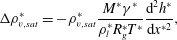 $$\begin{eqnarray}\unicode[STIX]{x0394}\unicode[STIX]{x1D70C}_{v,sat}^{\ast }=-\unicode[STIX]{x1D70C}_{v,sat}^{\ast }\frac{M^{\ast }\unicode[STIX]{x1D6FE}^{\ast }}{\unicode[STIX]{x1D70C}_{l}^{\ast }R_{g}^{\ast }T^{\ast }}\frac{\text{d}^{2}h^{\ast }}{\text{d}x^{\ast 2}},\end{eqnarray}$$
which is here written in a linearised form using a realistic simplifying assumption
 $\unicode[STIX]{x0394}\unicode[STIX]{x1D70C}_{v,sat}^{\ast }\ll \unicode[STIX]{x1D70C}_{v,sat}^{\ast }$
(see below). The boundary condition for
 $\unicode[STIX]{x1D70C}_{v}^{\ast }$
at the film is then given by
 $\unicode[STIX]{x1D70C}_{v}^{\ast }=\unicode[STIX]{x1D70C}_{v,sat}^{\ast }+\unicode[STIX]{x0394}\unicode[STIX]{x1D70C}_{v,sat}^{\ast }$
at
 $\unicode[STIX]{x1D711}=0$
(with
 $x^{\ast }\equiv r^{\ast }$
at
 $\unicode[STIX]{x1D711}=0$
). Note that
 $\unicode[STIX]{x0394}\unicode[STIX]{x1D70C}_{v,sat}^{\ast }\rightarrow 0$
away from the microregion, as
 $x^{\ast }\rightarrow +\infty$
, together with
 $\text{d}^{2}h^{\ast }/\text{d}x^{\ast 2}\rightarrow 0$
. Thus, the usual saturation condition
 $\unicode[STIX]{x1D70C}_{v}^{\ast }=\unicode[STIX]{x1D70C}_{v,sat}^{\ast }$
, free from the Kelvin effect, is automatically recovered towards the macroscopic part of the system.
Far away from the contact-line microregion (
 $r^{\ast }\rightarrow +\infty$
), the vapour concentration behaves as
 $$\begin{eqnarray}\unicode[STIX]{x1D70C}_{v}^{\ast }\sim \unicode[STIX]{x1D70C}_{v,sat}^{\ast }-2\frac{\unicode[STIX]{x1D70C}_{v,sat}^{\ast }-\unicode[STIX]{x1D70C}_{v,\infty }^{\ast }}{\ell ^{\ast 1/2}}r^{\ast 1/2}\sin \frac{\unicode[STIX]{x1D711}}{2}.\end{eqnarray}$$
The right-hand side of (2.3) satisfies
 $\unicode[STIX]{x1D6FB}^{\ast 2}\unicode[STIX]{x1D70C}_{v}^{\ast }=0$
and the boundary conditions
 $\unicode[STIX]{x2202}\unicode[STIX]{x1D70C}_{v}^{\ast }/\unicode[STIX]{x2202}\unicode[STIX]{x1D711}=0$
at
 $\unicode[STIX]{x1D711}=\unicode[STIX]{x03C0}$
and
 $\unicode[STIX]{x1D70C}_{v}^{\ast }=\unicode[STIX]{x1D70C}_{v,sat}^{\ast }$
at
 $\unicode[STIX]{x1D711}=0$
. It is a ‘corner solution’ with the lowest possible positive power of
 $r^{\ast }$
. Physically, it represents an intermediate asymptotic between the microregion and the macroscopic zone. (A more detailed discussion of how we arrive at a relation like (2.3) is given by Morris (Reference Morris2014).) The behaviour of the phase-change flux corresponding to (2.3) is just
 $j^{\ast }\sim D_{g}^{\ast }(\unicode[STIX]{x1D70C}_{v,sat}^{\ast }-\unicode[STIX]{x1D70C}_{v,\infty }^{\ast })/(\ell ^{\ast }x^{\ast })^{1/2}$
as
 $x^{\ast }\rightarrow +\infty$
. Here
 $\ell ^{\ast }$
is a macroscopic length, which in the case of a thin sessile drop in an isothermal quasi-steady diffusion-limited regime of phase change is equal to (cf. e.g. Popov Reference Popov2005)
 $$\begin{eqnarray}\ell ^{\ast }={\textstyle \frac{1}{2}}\unicode[STIX]{x03C0}^{2}R_{c}^{\ast },\end{eqnarray}$$
where
 $R_{c}^{\ast }$
is the contact radius of the sessile drop. The vapour density at infinity within the macroscopic configuration (i.e. far away from the sessile drop) is denoted by
 $\unicode[STIX]{x1D70C}_{v,\infty }^{\ast }$
. We have global evaporation for
 $\unicode[STIX]{x1D70C}_{v,sat}^{\ast }>\unicode[STIX]{x1D70C}_{v,\infty }^{\ast }$
(undersaturated atmosphere), global condensation for
 $\unicode[STIX]{x1D70C}_{v,sat}^{\ast }<\unicode[STIX]{x1D70C}_{v,\infty }^{\ast }$
(oversaturated atmosphere) and no global phase change for
 $\unicode[STIX]{x1D70C}_{v,sat}^{\ast }=\unicode[STIX]{x1D70C}_{v,\infty }^{\ast }$
(saturated atmosphere). In the case of a ‘dry’ atmosphere,
 $\unicode[STIX]{x1D70C}_{v,\infty }^{\ast }=0$
.
In a more general case, however,
 $\ell ^{\ast }$
is no longer given by (2.4) and must rather be determined individually for each particular macroscopic situation/configuration, which is beyond the scope of the present paper. In the present microregion analysis,
 $\ell ^{\ast }$
is treated as a known macroscopic input parameter. For instance, even in the realm of sessile/pendant drops, the concentration field can drastically be affected by buoyancy convection (cf. e.g. Dehaeck, Rednikov & Colinet Reference Dehaeck, Rednikov and Colinet2014). In such a case, a diffusion-limited regime is expected to persist just locally in the microscopic vicinity of the contact line, so that (2.3) and our microregion approach are still valid and
 $\ell ^{\ast }$
can in principle be determined. (In the most general case, however, when the meaning of
 $\unicode[STIX]{x1D70C}_{v,\infty }^{\ast }$
may not be well defined, it would be more appropriate to render (2.3) in terms of a single prefactor, say
 $B^{\ast }$
, in lieu of
 $(\unicode[STIX]{x1D70C}_{v,sat}^{\ast }-\unicode[STIX]{x1D70C}_{v,\infty }^{\ast })/\ell ^{\ast 1/2}$
, so that it would rather be
 $B^{\ast }$
a macroscopic input parameter in our microregion problem.)
The following observation is due here. As
 $\ell ^{\ast }$
is a macroscopic length, we expect that
 $r^{\ast }\ll \ell ^{\ast }$
in the microregion. On the other hand,
 $(\unicode[STIX]{x1D70C}_{v,sat}^{\ast }-\unicode[STIX]{x1D70C}_{v,\infty }^{\ast })$
is generally of the order of
 $\unicode[STIX]{x1D70C}_{v,sat}^{\ast }$
. Then, we see that the second term on the right-hand side of (2.3) is much smaller than the first one. In other words, it is merely a small variation of
 $\unicode[STIX]{x1D70C}_{v}^{\ast }$
about
 $\unicode[STIX]{x1D70C}_{v,sat}^{\ast }$
(near-saturated atmosphere) that is incited by (2.3) in the microregion. This is coherent with using just a linearised form of the Kelvin equation (2.2), Morris (Reference Morris2014) arriving at the same conclusion. Furthermore, this makes it appropriate to work in terms of the corresponding deviation of the vapour density:
 $$\begin{eqnarray}\tilde{\unicode[STIX]{x1D70C}}_{v}^{\ast }\equiv \unicode[STIX]{x1D70C}_{v}^{\ast }-\unicode[STIX]{x1D70C}_{v,sat}^{\ast }.\end{eqnarray}$$
We now recapitulate the problem in the gas phase formulated in the present subsection, simultaneously rendering it in terms of
 $\tilde{\unicode[STIX]{x1D70C}}_{v}^{\ast }$
defined in (2.5):
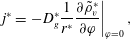 $$\begin{eqnarray}\displaystyle & \displaystyle j^{\ast }=\left.-D_{g}^{\ast }\frac{1}{r^{\ast }}\frac{\unicode[STIX]{x2202}\tilde{\unicode[STIX]{x1D70C}}_{v}^{\ast }}{\unicode[STIX]{x2202}\unicode[STIX]{x1D711}}\right|_{\unicode[STIX]{x1D711}=0}, & \displaystyle\end{eqnarray}$$
 $$\begin{eqnarray}\displaystyle & \unicode[STIX]{x1D6FB}^{\ast 2}\tilde{\unicode[STIX]{x1D70C}}_{v}^{\ast }=0, & \displaystyle\end{eqnarray}$$
 $$\begin{eqnarray}\displaystyle & \displaystyle \tilde{\unicode[STIX]{x1D70C}}_{v}^{\ast }=-\unicode[STIX]{x1D70C}_{v,sat}^{\ast }\frac{M^{\ast }\unicode[STIX]{x1D6FE}^{\ast }}{\unicode[STIX]{x1D70C}_{l}^{\ast }R_{g}^{\ast }T^{\ast }}\frac{\text{d}^{2}h^{\ast }}{\text{d}x^{\ast 2}}\quad \text{at}~\unicode[STIX]{x1D711}=0, & \displaystyle\end{eqnarray}$$
 $$\begin{eqnarray}\displaystyle & \unicode[STIX]{x2202}\tilde{\unicode[STIX]{x1D70C}}_{v}^{\ast }/\unicode[STIX]{x2202}\unicode[STIX]{x1D711}=0\quad \text{at}~\unicode[STIX]{x1D711}=\unicode[STIX]{x03C0}, & \displaystyle\end{eqnarray}$$
 $$\begin{eqnarray}\displaystyle & \displaystyle \tilde{\unicode[STIX]{x1D70C}}_{v}^{\ast }\sim -2\frac{\unicode[STIX]{x1D70C}_{v,sat}^{\ast }-\unicode[STIX]{x1D70C}_{v,\infty }^{\ast }}{\ell ^{\ast 1/2}}r^{\ast 1/2}\sin \frac{\unicode[STIX]{x1D711}}{2}\quad \text{as}~r^{\ast }\rightarrow \infty . & \displaystyle\end{eqnarray}$$
This concludes the formulation of the overall microregion problem developed in §§ 2.1–2.3, which we shall recapitulate in § 2.4 in dimensionless terms. Before proceeding to this dimensionless formulation, we shall dwell upon a number of relevant points.
First, note that without the Kelvin effect, i.e. if the boundary condition (2.8) were replaced with simply
 $\tilde{\unicode[STIX]{x1D70C}}_{v}^{\ast }=0$
, the right-hand side of (2.10) would be an exact solution of the problem for
 $\tilde{\unicode[STIX]{x1D70C}}_{v}^{\ast }$
. On account of (2.6), this would yield a phase-change flux
 $j^{\ast }=D_{g}^{\ast }(\unicode[STIX]{x1D70C}_{v,sat}^{\ast }-\unicode[STIX]{x1D70C}_{v,\infty }^{\ast })/(\ell ^{\ast }x^{\ast })^{1/2}$
valid throughout, with a classical integrable divergence as
 $x^{\ast }\rightarrow 0$
(Deegan et al.
Reference Deegan, Bakajin, Dupont, Huber, Nagel and Witten1997; Popov Reference Popov2005). This simple expression for the flux may well be appropriate in microregion studies (Berteloot et al.
Reference Berteloot, Pham, Daerr, Lequeux and Limat2008; Pham et al.
Reference Pham, Berteloot, Lequeux and Limat2010; Colinet & Rednikov Reference Colinet and Rednikov2011; Saxton et al.
Reference Saxton, Whiteley, Vella and Oliver2016) provided that there are other factors (viz. the disjoining pressure, or the Navier slip) taking care of contact-line singularities. For the present configuration (contact line with Young’s angle, no disjoining pressure, no slip), it would lead to film-flow singularities even stronger (as detailed e.g. by Rednikov & Colinet Reference Rednikov and Colinet2013) than those associated with contact-line motion. This underscores the crucial role of the Kelvin effect here. In the presence of the Kelvin effect,
 $j^{\ast }\sim D_{g}^{\ast }(\unicode[STIX]{x1D70C}_{v,sat}^{\ast }-\unicode[STIX]{x1D70C}_{v,\infty }^{\ast })/(\ell ^{\ast }x^{\ast })^{1/2}$
remains just a behaviour as
 $x^{\ast }\rightarrow +\infty$
, whereas in the rest of the microregion
 $j^{\ast }$
deviates from it and, as we shall see, can in principle even change sign. In other words, the direction of the local phase change (the sign of
 $j^{\ast }$
at any given
 $x^{\ast }$
) need not coincide with the direction of the global phase change (the sign of
 $j^{\ast }$
as
 $x^{\ast }\rightarrow +\infty$
).
Second, in the particular case of a saturated ambient atmosphere (
 $\unicode[STIX]{x1D70C}_{v,sat}^{\ast }=\unicode[STIX]{x1D70C}_{v,\infty }^{\ast }$
), when the condition (2.10) becomes homogeneous, the solution is generally not given by
 $\tilde{\unicode[STIX]{x1D70C}}_{v}^{\ast }=0$
and
 $j^{\ast }=0$
. This is in view of the Kelvin effect that can still be activated by contact-line motion and the associated film deformation, cf. (2.8).
Third, the trivial solution corresponding to thermodynamic equilibrium in a saturated atmosphere (
 $\unicode[STIX]{x1D70C}_{v,sat}^{\ast }=\unicode[STIX]{x1D70C}_{v,\infty }^{\ast }$
) for an immobile contact line (
 $c^{\ast }=0$
) is just given by
 $\tilde{\unicode[STIX]{x1D70C}}_{v}^{\ast }=0$
(i.e.
 $\unicode[STIX]{x1D70C}_{v}^{\ast }=\unicode[STIX]{x1D70C}_{v,sat}^{\ast }$
),
 $j^{\ast }=0$
and
 $h^{\ast }=\unicode[STIX]{x1D703}_{Y}\,x^{\ast }$
throughout. It does not make sense in the perfect-wetting case (
 $\unicode[STIX]{x1D703}_{Y}=0$
) however, which is consistent with the expected indefinite spreading.
Finally, note that (2.6) actually introduces a non-local operator from the viewpoint of the film equation (2.1). Indeed, the value of
 $j^{\ast }$
at each point depends, by means of the vapour concentration field, on the overall film configuration, and not just on its state at this point. In contrast, no non-local operators occur in the pure-vapour counterpart of the present problem (cf. e.g. Rednikov & Colinet Reference Rednikov and Colinet2013).
2.4 Dimensionless formulation summary and the scales
Let the asterisk or absence thereof distinguish between the dimensional and dimensionless quantities, respectively, while the square brackets around a quantity refer to its scale:
 $$\begin{eqnarray}f=f^{\ast }/[f].\end{eqnarray}$$
In dimensionless form, the stationary microregion formulation of §§ 2.2, 2.3 can be rewritten as (explanations below)
 $$\begin{eqnarray}\displaystyle c\frac{\text{d}h}{\text{d}x}+\frac{\text{d}}{\text{d}x}\left(h^{3}\frac{\text{d}^{3}h}{\text{d}x^{3}}\right)+j=0\quad (x>0),\end{eqnarray}$$
 $$\begin{eqnarray}h=0,\quad \text{d}h/\text{d}x=\unicode[STIX]{x1D717}_{Y}\quad \text{at }x=0,\end{eqnarray}$$
 $$\begin{eqnarray}h\rightarrow +\infty ,\quad \text{d}^{2}h/\text{d}x^{2}=0\quad \text{as}~x\rightarrow +\infty ,\end{eqnarray}$$
 $$\begin{eqnarray}\frac{\unicode[STIX]{x2202}^{2}\tilde{\unicode[STIX]{x1D70C}}_{v}}{\unicode[STIX]{x2202}r^{2}}+\frac{1}{r}\frac{\unicode[STIX]{x2202}\tilde{\unicode[STIX]{x1D70C}}_{v}}{\unicode[STIX]{x2202}r}+\frac{1}{r^{2}}\frac{\unicode[STIX]{x2202}^{2}\tilde{\unicode[STIX]{x1D70C}}_{v}}{\unicode[STIX]{x2202}\unicode[STIX]{x1D711}^{2}}=0\quad (r>0,\,0<\unicode[STIX]{x1D711}<\unicode[STIX]{x03C0}),\end{eqnarray}$$
 $$\begin{eqnarray}j=-\frac{1}{x}\frac{\unicode[STIX]{x2202}\tilde{\unicode[STIX]{x1D70C}}_{v}}{\unicode[STIX]{x2202}\unicode[STIX]{x1D711}},\quad \tilde{\unicode[STIX]{x1D70C}}_{v}=-3{\mathcal{K}}\frac{\text{d}^{2}h}{\text{d}x^{2}}\quad \text{at}~\unicode[STIX]{x1D711}=0\quad (x\equiv r>0),\end{eqnarray}$$
 $$\begin{eqnarray}\displaystyle & \unicode[STIX]{x2202}\tilde{\unicode[STIX]{x1D70C}}_{v}/\unicode[STIX]{x2202}\unicode[STIX]{x1D711}=0\quad \text{at}~\unicode[STIX]{x1D711}=\unicode[STIX]{x03C0}\quad (r>0), & \displaystyle\end{eqnarray}$$
 $$\begin{eqnarray}\displaystyle & \displaystyle \tilde{\unicode[STIX]{x1D70C}}_{v}\sim -2Er^{1/2}\sin \frac{\unicode[STIX]{x1D711}}{2}\quad \text{as}~r\rightarrow +\infty \quad (0\leqslant \unicode[STIX]{x1D711}\leqslant \unicode[STIX]{x03C0}), & \displaystyle\end{eqnarray}$$
 $$\begin{eqnarray}\displaystyle & \tilde{\unicode[STIX]{x1D70C}}_{v}<\infty \quad \text{as}~r\rightarrow 0\quad (0\leqslant \unicode[STIX]{x1D711}\leqslant \unicode[STIX]{x03C0}), & \displaystyle\end{eqnarray}$$
with the dimensionless numbers
 $$\begin{eqnarray}c=\frac{c^{\ast }}{[c]}=3\,Ca\,\unicode[STIX]{x1D716}^{-3},\quad \unicode[STIX]{x1D717}_{Y}=\unicode[STIX]{x1D703}_{Y}\unicode[STIX]{x1D716}^{-1},\quad E=3\,Ca_{evap}\,\unicode[STIX]{x1D716}^{-4},\end{eqnarray}$$
 $$\begin{eqnarray}{\mathcal{K}}=\frac{\unicode[STIX]{x1D6FF}^{\ast 2}}{\unicode[STIX]{x1D716}^{3}[x]^{2}},\quad Ca=\frac{\unicode[STIX]{x1D707}_{l}^{\ast }c^{\ast }}{\unicode[STIX]{x1D6FE}^{\ast }},\quad Ca_{evap}=\frac{\unicode[STIX]{x1D707}_{l}^{\ast }D_{g}^{\ast }(\unicode[STIX]{x1D70C}_{v,sat}^{\ast }-\unicode[STIX]{x1D70C}_{v,\infty }^{\ast })}{\unicode[STIX]{x1D70C}_{l}^{\ast }\unicode[STIX]{x1D6FE}^{\ast }\ell ^{\ast 1/2}[x]^{1/2}},\end{eqnarray}$$
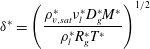 $$\begin{eqnarray}\unicode[STIX]{x1D6FF}^{\ast }=\left(\frac{\unicode[STIX]{x1D70C}_{v,sat}^{\ast }\unicode[STIX]{x1D708}_{l}^{\ast }D_{g}^{\ast }M^{\ast }}{\unicode[STIX]{x1D70C}_{l}^{\ast }R_{g}^{\ast }T^{\ast }}\right)^{1/2}\end{eqnarray}$$
(
 $\unicode[STIX]{x1D708}_{l}^{\ast }=\unicode[STIX]{x1D707}_{l}^{\ast }/\unicode[STIX]{x1D70C}_{l}^{\ast }$
being the kinematic viscosity of the liquid) is introduced for future convenience. The quantities are rendered dimensionless, cf. the rule (2.11), using the following scales:
 $$\begin{eqnarray}[h]=\unicode[STIX]{x1D716}[x],\quad [r]=[x],\quad [c]=\frac{\unicode[STIX]{x1D6FE}^{\ast }}{3\unicode[STIX]{x1D707}_{l}^{\ast }}\unicode[STIX]{x1D716}^{3},\quad [j]=\frac{\unicode[STIX]{x1D70C}_{l}^{\ast }\unicode[STIX]{x1D6FE}^{\ast }}{3\unicode[STIX]{x1D707}_{l}^{\ast }}\unicode[STIX]{x1D716}^{4},\quad [\tilde{\unicode[STIX]{x1D70C}}_{v}]=\frac{[j][x]}{D_{g}^{\ast }},\end{eqnarray}$$
where
 $[x]$
is for the moment left unspecified, and recall that the film-slope parameter
 $\unicode[STIX]{x1D716}$
, cf. § 2.1, is not yet specified either.
The liquid-film part of the formulation, considered in § 2.2, here leads to (2.12)–(2.14), where in particular (2.12) originates from (2.1) on account of looking for stationary microregion profiles translating at a constant velocity
 $c^{\ast }$
. Recall that
 $c^{\ast }$
is a given (input) parameter within the microregion problem, and not an unknown. That is why
 $c$
appears among the dimensionless numbers (2.20). The diffusional/Kelvin part of the formulation, cf. § 2.3, translates in dimensionless form into (2.15)–(2.19).
Among the dimensionless numbers (2.20),
 $\unicode[STIX]{x1D717}_{Y}$
is the rescaled Young’s angle,
 $E$
is the evaporation number,
 ${\mathcal{K}}$
is (what we refer to as) the Kelvin number,
 $Ca$
is the capillary number and
 $Ca_{evap}$
is the evaporation capillary number. They are defined so as to correspond as much as possible to their counterparts in the pure-vapour case considered elsewhere (Rednikov & Colinet Reference Rednikov and Colinet2013), although the expressions may be quite different. The length parameter
 $\unicode[STIX]{x1D6FF}^{\ast }$
is associated with the Kelvin effect and also has its pure-vapour counterpart (Rednikov & Colinet Reference Rednikov and Colinet2013). The dimensionless numbers
 $c$
,
 $\unicode[STIX]{x1D717}_{Y}$
,
 $E$
and
 ${\mathcal{K}}$
, immediately appearing in the dimensionless formulation (2.12)–(2.19), are generally assumed to be
 $O(1)$
, whereas then
 $\unicode[STIX]{x1D703}_{Y}\ll 1$
,
 $Ca\ll 1$
and
 $Ca_{evap}\ll 1$
in keeping within (2.20) with the general premise
 $\unicode[STIX]{x1D716}\ll 1$
, cf. § 2.1, relied upon here.
Other angle quantities (viz.
 $\unicode[STIX]{x1D703}_{app}$
,
 $\unicode[STIX]{x1D703}_{mic}$
,
 $\unicode[STIX]{x1D703}_{evap}$
and
 $\unicode[STIX]{x1D703}_{eff}$
), to be introduced later when appropriate, are also rescaled with
 $\unicode[STIX]{x1D716}$
in the same way as
 $\unicode[STIX]{x1D703}_{Y}$
in (2.20b
):
 $$\begin{eqnarray}\unicode[STIX]{x1D703}_{Y}=\unicode[STIX]{x1D716}\unicode[STIX]{x1D717}_{Y},\quad \unicode[STIX]{x1D703}_{app}=\unicode[STIX]{x1D716}\unicode[STIX]{x1D717}_{app},\quad \unicode[STIX]{x1D703}_{mic}=\unicode[STIX]{x1D716}\unicode[STIX]{x1D717}_{mic},\quad \unicode[STIX]{x1D703}_{evap}=\unicode[STIX]{x1D716}\unicode[STIX]{x1D717}_{evap},\quad \unicode[STIX]{x1D703}_{eff}=\unicode[STIX]{x1D716}\unicode[STIX]{x1D717}_{eff},\end{eqnarray}$$
where the
 $\unicode[STIX]{x1D703}$
values are in radians, and the
 $\unicode[STIX]{x1D717}$
values are generally assumed
 $O(1)$
.
The choice of the two remaining non-specified quantities,
 $[x]$
and
 $\unicode[STIX]{x1D716}$
, is accomplished according to the principle of dominant balance. As the Kelvin effect is the key in our problem, we here choose
 ${\mathcal{K}}\equiv 1$
throughout, so that one of the two ends up specified (say
 $[x]$
, but not yet
 $\unicode[STIX]{x1D716}$
). Hence, on account of (2.20d
) and (2.22a
), we can write
 $$\begin{eqnarray}[x]=\unicode[STIX]{x1D6FF}^{\ast }/\unicode[STIX]{x1D716}^{3/2},\quad [h]=\unicode[STIX]{x1D6FF}^{\ast }/\unicode[STIX]{x1D716}^{1/2}\quad (\text{scaling}~{\mathcal{K}}\equiv 1).\end{eqnarray}$$
The length scale
 $[x]$
appearing in (2.24a
) actually represents the longitudinal extent of the Kelvin-effect-determined microregion, i.e. the length scale at which contact-line singularities are to be resolved thanks to the Kelvin effect. The parameter
 $\unicode[STIX]{x1D6FF}^{\ast }$
typically proves to be a subnanometric quantity (e.g. with
 $\unicode[STIX]{x1D70C}_{v,sat}^{\ast }\sim 0.2~\text{kg}~\text{m}^{-3}$
,
 $\unicode[STIX]{x1D708}_{l}^{\ast }\sim 10^{-6}~\text{m}^{2}~\text{s}^{-1}$
,
 $D_{g}^{\ast }\sim 10^{-5}~\text{m}^{2}~\text{s}^{-1}$
,
 $M^{\ast }\sim 0.05~\text{kg}~\text{mol}^{-1}$
,
 $\unicode[STIX]{x1D70C}_{l}^{\ast }\sim 1000~\text{kg}~\text{m}^{-3}$
,
 $R_{g}^{\ast }=8.31~\text{J}~\text{mol}^{-1}~\text{K}^{-1}$
,
 $T^{\ast }\sim 300~\text{K}$
, we obtain
 $\unicode[STIX]{x1D6FF}^{\ast }\sim 0.2~\text{nm}$
) or at most a nanometric one (the latter notably for strongly volatile liquids with large molecules such as e.g. FC-72 or HFE-7100). Then, assuming for estimation purposes
 $\unicode[STIX]{x1D716}\sim 0.1$
, the microregion length scale
 $[x]$
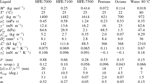
must be of the order of tens of nanometres. This is not surprising, since the Kelvin effect typically requires rather large curvatures to become apparent. For further estimations, see appendix B and table 2.
To recapitulate, it is ultimately the dimensionless problem (2.12)–(2.19) with
 ${\mathcal{K}}\equiv 1$
that is solved in the present paper. The quantities are made dimensionless with the scales defined by (2.21), (2.22) and (2.24), implying the rule (2.11). The dimensionless numbers are given in (2.20). There just remains the slope parameter
 $\unicode[STIX]{x1D716}$
still to be defined, which will be accomplished separately in each case studied using the dominant balance at hand.
Finally, it is worth emphasising that it is here a successful construction of the solution to the formulated problem that will eventually serve as a proof of the possibility of resolving contact-line singularities by means of the Kelvin effect only. We shall also monitor the shear stress on the substrate, a dimensionless expression for which is given in accordance with (2.1d ) and (2.24) by
 $$\begin{eqnarray}\unicode[STIX]{x1D70E}_{\unicode[STIX]{x1D70F}}=h\frac{\text{d}^{3}h}{\text{d}x^{3}},\quad [\unicode[STIX]{x1D70E}_{\unicode[STIX]{x1D70F}}]=\frac{\unicode[STIX]{x1D6FE}^{\ast }}{\unicode[STIX]{x1D6FF}^{\ast }}\,\unicode[STIX]{x1D716}^{7/2},\end{eqnarray}$$
and whose appropriate behaviour as
 $x\rightarrow 0$
will confirm the singularity resolution.
3 Cases studied
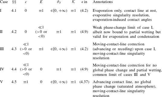
Table 1 summarises at a glance the (parametric) study cases to be developed, providing further details in terms of the quantities (2.20) to what was already announced at the end of § 1.
We note that cases I, III and V involve as an input a dimensionless number that can in principle take any value in the interval
 $[0,+\infty )$
(here always the rescaled Young’s angle
 $\unicode[STIX]{x1D717}_{Y}$
). Cases II, III and IV, implying either a small (
 $\ll 1$
) or a large (
 $\gg 1$
) parameter, will be treated by means a corresponding perturbation analysis. We also anticipate that the perturbation results to be obtained for
 $c\ll 1$
will actually be valid for both advancing (
 $c>0$
) and receding (
 $c<0$
) contact lines. For
 $c=O(1)$
, however, the study will here be limited to the advancing case (
 $c>0$
) and carried out within the scaling
 $c\equiv 1$
. Similarly, the
 $E\ll 1$
perturbation results will actually be valid for both global evaporation (
 $E>0$
) and global condensation (
 $E<0$
), although for
 $E=O(1)$
the study will be limited to the evaporation case (
 $E>0$
) and realised within the scaling
 $E\equiv 1$
.
Cases studied and scalings chosen for each of them. With the indicated expressions for
 $\unicode[STIX]{x1D716}$
, the scales are fully defined from (2.21), (2.22) and (2.24), the (remaining) dimensionless numbers from (2.20), and the rescaled angle quantities versus the original ones from (2.23).
4 Results and discussion
4.1 Purely evaporative case and evaporation-induced contact angles (case I)
The problem studied in the present subsection belongs to a paradigmatic purely evaporative microregion setting, with
 $\unicode[STIX]{x1D70C}_{v,sat}^{\ast }>\unicode[STIX]{x1D70C}_{v,\infty }^{\ast }$
and the contact-line velocity either vanishing (
 $c=0$
), or just insignificant as compared to the evaporation-induced liquid velocity in the microregion (
 $c\ll 1$
). In either case, the leading-order approximation boils here down to a contact line at rest, with
 $$\begin{eqnarray}c=0.\end{eqnarray}$$
The main interest of such a consideration is arguably calculating a finite value of the evaporation-induced apparent contact angle, here accomplished in the Kelvin-only setting. With such a focus, we choose
 $E\equiv 1$
for a final specification of the film-slope parameter
 $\unicode[STIX]{x1D716}$
(cf. the end of § 2.4). Then, using (2.24) and the expression for
 $E$
from (2.20), we deduce
 $$\begin{eqnarray}\unicode[STIX]{x1D716}=\left(\frac{3(\unicode[STIX]{x1D70C}_{v,sat}^{\ast }-\unicode[STIX]{x1D70C}_{v,\infty }^{\ast })\unicode[STIX]{x1D708}_{l}^{\ast }D_{g}^{\ast }}{\unicode[STIX]{x1D6FE}^{\ast }\ell ^{\ast 1/2}\unicode[STIX]{x1D6FF}^{\ast 1/2}}\right)^{4/13}\quad (\text{scaling}~{\mathcal{K}}\equiv 1,\,E\equiv 1),\end{eqnarray}$$
characterising the order of magnitude of the evaporation-induced angles, where the length
 $\unicode[STIX]{x1D6FF}^{\ast }$
is given by (2.21). Using the typical values
 $(\unicode[STIX]{x1D70C}_{v,sat}^{\ast }-\unicode[STIX]{x1D70C}_{v,\infty }^{\ast })\sim 0.2~\text{kg}~\text{m}^{-3}$
(
 ${\sim}20\,\%$
of the normal air density),
 $\unicode[STIX]{x1D708}_{l}^{\ast }\sim 10^{-6}~\text{m}^{2}~\text{s}^{-1}$
,
 $D_{g}^{\ast }\sim 10^{-5}~\text{m}^{2}~\text{s}^{-1}$
,
 $\unicode[STIX]{x1D6FE}^{\ast }\sim 20~\text{mN}~\text{m}^{-1}$
,
 $\unicode[STIX]{x1D6FF}^{\ast }\sim 1~\text{nm}$
and
 $\ell ^{\ast }\sim 1~\text{mm}$
, we estimate
 $\unicode[STIX]{x1D716}\sim 0.1$
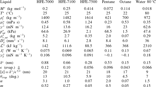
, which is a sufficiently small value consistent with our overall approach. Further estimations can be found in appendix B and table 2.
Material properties and the resulting values of certain parameters, such as (2.21), (2.24a
), (4.2), (4.6b
), (A 1) and (A 2), for a number of liquids. Here
 $\unicode[STIX]{x1D708}_{l}^{\ast }=\unicode[STIX]{x1D707}_{l}^{\ast }/\unicode[STIX]{x1D70C}_{l}^{\ast }$
and
 $\unicode[STIX]{x1D70C}_{v,sat}^{\ast }=p_{sat}^{\ast }M^{\ast }/R_{g}^{\ast }T^{\ast }$
. For
 $\unicode[STIX]{x1D716}$
and
 $[x]$
, the evaporation-induced values (cf. § 4.1) are estimated assuming
 $\ell ^{\ast }$
as for a thin sessile drop in a diffusion-limited regime (2.4) with
 $R_{c}=2~\text{mm}$
.
Thus, the problem solved here is given by (2.12)–(2.19) with
 ${\mathcal{K}}\equiv 1$
,
 $E\equiv 1$
and
 $c=0$
. The only input parameter remaining in the formulation is the rescaled Young’s angle
 $\unicode[STIX]{x1D717}_{Y}=\unicode[STIX]{x1D703}_{Y}/\unicode[STIX]{x1D716}$
, where
 $\unicode[STIX]{x1D716}$
is given by (4.2), and which can in principle adopt any non-negative value.
With
 $c=0$
(but not for
 $c\neq 0$
, see § 4.3), the condition (2.14) gives rise to a constant-slope behaviour
 $$\begin{eqnarray}h\sim \unicode[STIX]{x1D717}_{mic}x\quad \text{as}~x\rightarrow +\infty ,\end{eqnarray}$$
where
 $\unicode[STIX]{x1D717}_{mic}$
is a coefficient, which clearly amounts to the apparent contact angle as seen at larger length scales beyond the microregion. (The subscript ‘
 $mic$
’ intends to convey the idea of a ‘microregion angle’ or an ‘angle of the contact-line microstructure’ or rather simply a ‘microscopic angle’.) More elaborately, one can establish from (2.16) and (2.18) with
 $E\equiv 1$
that
 $j\sim 1/x^{1/2}$
to leading order as
 $x\rightarrow +\infty$
, and then from (2.12) and (4.3) a more detailed behaviour
 $h\sim \unicode[STIX]{x1D717}_{mic}x-16x^{1/2}/3\unicode[STIX]{x1D717}_{mic}^{3}$
as
 $x\rightarrow +\infty$
. The second term proves to be just a correction, which confirms the consistency of the leading-order asymptotic (4.3). Further development of such coordinate expansions is provided in appendix C. The quantity
 $\unicode[STIX]{x1D717}_{mic}$
is not a priori known and must be obtained as part of the solution.
The role of the Kelvin effect is instrumental in that it allows a non-singular behaviour at the other end of the domain, as confirmed by successfully developing the coordinate expansions
 $$\begin{eqnarray}h\sim \unicode[STIX]{x1D717}_{Y}x-{\textstyle \frac{1}{6}}C_{0}x^{2}-{\textstyle \frac{1}{18}}C_{1}x^{3}+\cdots \quad \text{as}~x\rightarrow 0,\end{eqnarray}$$
 $$\begin{eqnarray}\displaystyle \tilde{\unicode[STIX]{x1D70C}}_{v} & {\sim} & \displaystyle C_{0}+C_{1}r\cos \unicode[STIX]{x1D711}+C_{2}r^{2}\cos 2\unicode[STIX]{x1D711}-\frac{\unicode[STIX]{x1D717}_{Y}^{3}C_{1}}{3\unicode[STIX]{x03C0}}r^{3}(\ln r\cos 3\unicode[STIX]{x1D711}-(\unicode[STIX]{x1D711}-\unicode[STIX]{x03C0})\sin 3\unicode[STIX]{x1D711})\nonumber\\ \displaystyle & & \displaystyle +\,C_{3}r^{3}\cos 3\unicode[STIX]{x1D711}+\cdots \quad \text{as}~r\rightarrow 0,\end{eqnarray}$$
where
 $C_{0}$
,
 $C_{1}$
, etc. are free coefficients to be determined as part of the solution, similarly to
 $\unicode[STIX]{x1D717}_{mic}$
. According to (4.4),
 $\text{d}^{2}h/\text{d}x^{2}$
and hence the pressure in the liquid, cf. (2.1c
), remains finite as
 $x\rightarrow 0$
. Furthermore, the derivative of the pressure is also finite. This can be compared with an
 $x^{-1}$
pressure divergence for the classical motion-related singularity (e.g. Huh & Scriven Reference Huh and Scriven1971; de Gennes Reference de Gennes1985; Rednikov & Colinet Reference Rednikov and Colinet2013). The local evaporation flux behaviour can be established from (4.5) and (2.16a
) yielding just
 $j\sim \unicode[STIX]{x1D717}_{Y}^{3}C_{1}x^{2}$
as
 $x\rightarrow 0$
. This smooth behaviour with
 $j=0$
at
 $x=0$
can in turn be contrasted with an evaporative singularity in the form an
 $x^{-1/2}$
flux divergence that would take place in the absence of the Kelvin effect (cf. § 2.3). We already had an occasion to mention that, unamended, this would result in an even stronger pressure divergence, as
 $x^{-3/2}$
, than for the classical motion-related singularity (cf. e.g. Rednikov & Colinet Reference Rednikov and Colinet2013). At last, given (4.4), the shear stress on the substrate (2.25a
) behaves as
 $\unicode[STIX]{x1D70E}_{\unicode[STIX]{x1D70F}}\sim -(1/3)\unicode[STIX]{x1D717}_{Y}C_{1}x$
as
 $x\rightarrow 0$
, being not merely integrable but also remarkably vanishing towards the contact line. Thus, we see that the evaporative singularity is indeed taken care of by the Kelvin effect, which is a first intended result of the analysis. We shall now see how the non-singular behaviour (4.4) and (4.5) shows itself within the numerical solution for the entire microregion.
In our numerical approach, the actual domain
 $0\leqslant r<+\infty$
,
 $0\leqslant \unicode[STIX]{x1D711}\leqslant \unicode[STIX]{x03C0}$
(with
 $x\equiv r$
at
 $\unicode[STIX]{x1D711}=0$
) is approximated by
 $r_{min}\leqslant r\leqslant r_{max}$
,
 $0\leqslant \unicode[STIX]{x1D711}\leqslant \unicode[STIX]{x03C0}$
, where
 $r_{min}$
and
 $r_{max}$
are sufficiently small and large values, respectively. The boundary conditions at
 $r=r_{min}$
are imposed with the help of the coordinate expansions (4.4) and (4.5). At
 $r=r_{max}$
, they are imposed using (C 1) and (C 2). The problem is discretised by finite differences on a uniform rectangular grid in terms of a logarithmic coordinate
 $\unicode[STIX]{x1D709}=\ln r$
and
 $\unicode[STIX]{x1D711}$
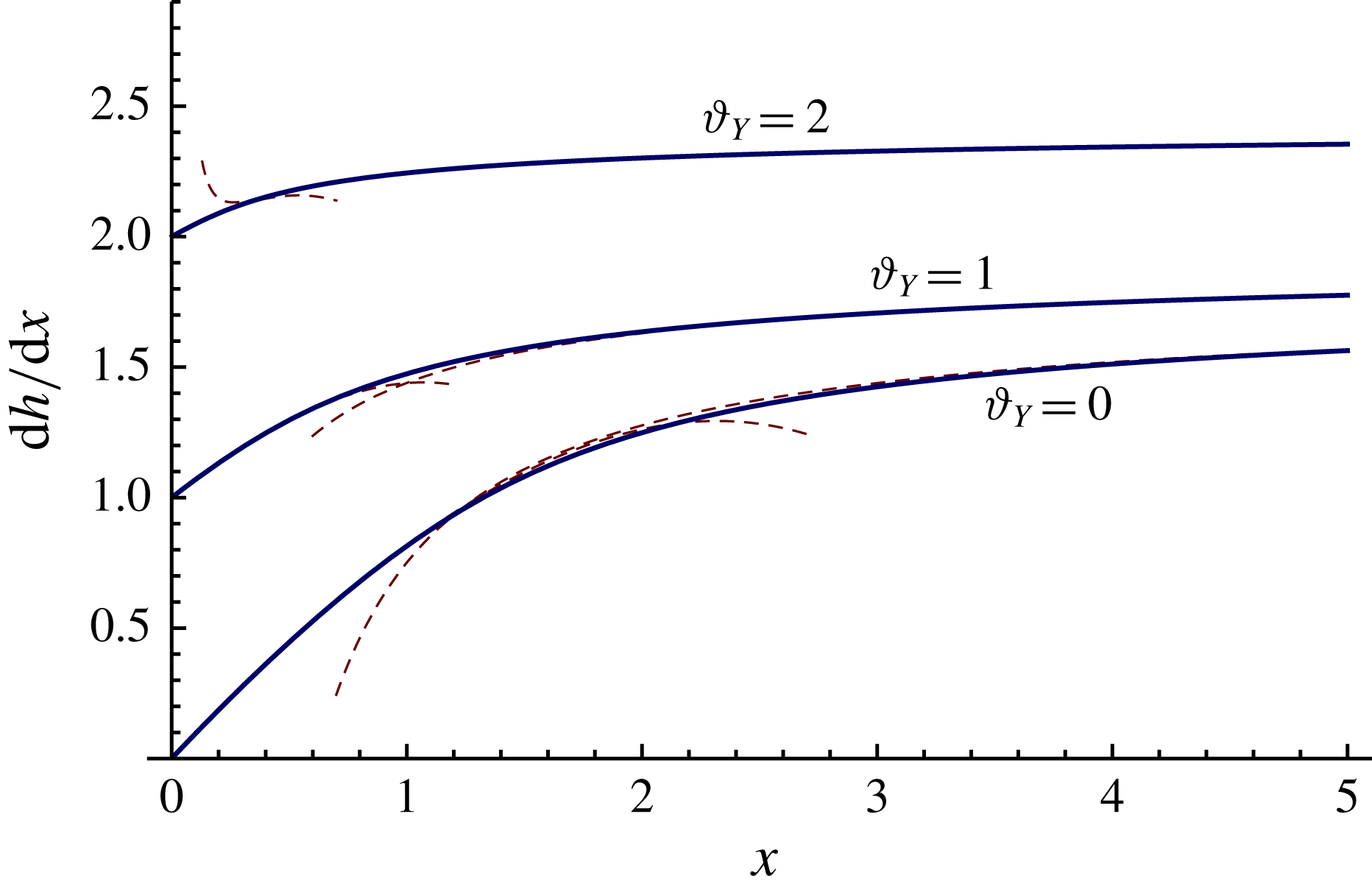
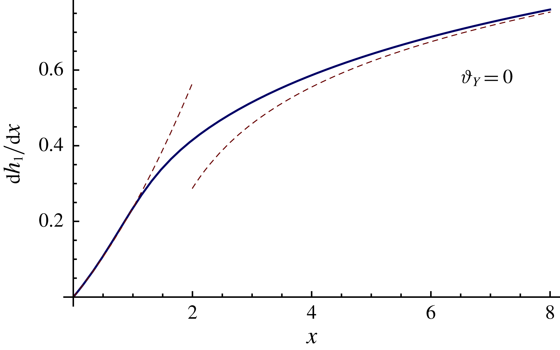
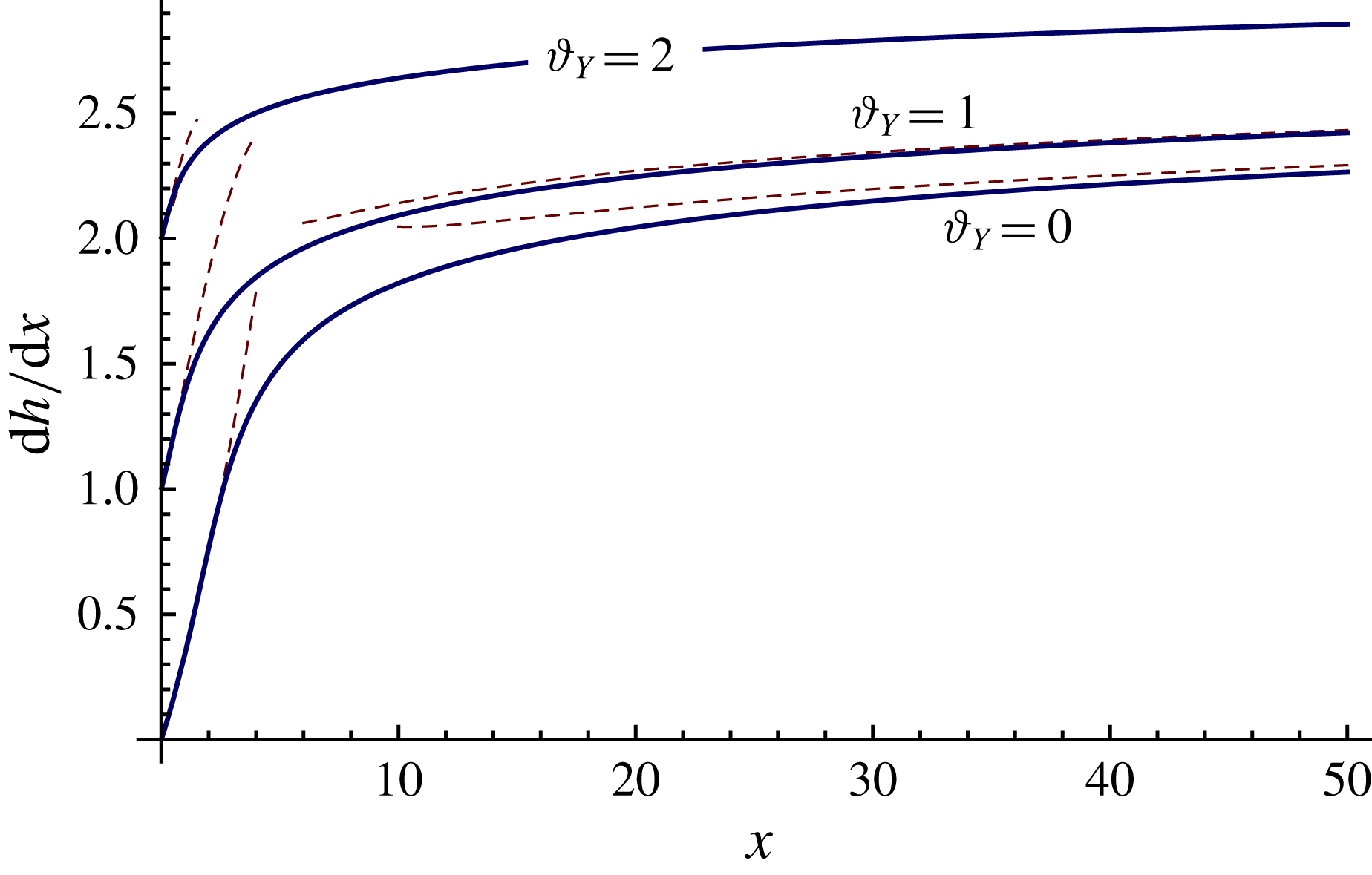
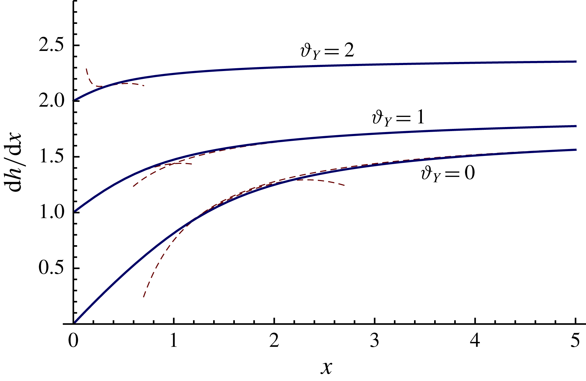
. Finally, we end up with a system of nonlinear algebraic equations for the values of the dependent variables at the grid points and the free coefficients in the retained terms of the coordinate expansions. It is solved using the FindRoot command in Mathematica®. A smooth solution is obtained, which, as illustrated in figure 2 for the film-slope profiles, conforms well to the coordinate expansions. The latter fact in particular ensures that the dependence of the results on the chosen values of
 $r_{min}$
and
 $r_{max}$
is not significant. The profiles manifest a monotonic increase of the slope from
 $\unicode[STIX]{x1D717}_{Y}$
at the tip of the film (the proper contact line) to eventually
 $\unicode[STIX]{x1D717}_{mic}$
as
 $x\rightarrow +\infty$
, as expected.
Film-slope profiles
 $\text{d}h/\text{d}x=\unicode[STIX]{x1D716}^{-1}\,\text{d}h^{\ast }/\text{d}x^{\ast }$
in the purely evaporative case (case I of table 1) for a number of values of the rescaled Young’s angle
 $\unicode[STIX]{x1D717}_{Y}=\unicode[STIX]{x1D716}^{-1}\unicode[STIX]{x1D703}_{Y}$
. Numerical results (solid lines) and the course of the corresponding coordinate expansions for small and large
 $x$
(dashed lines).
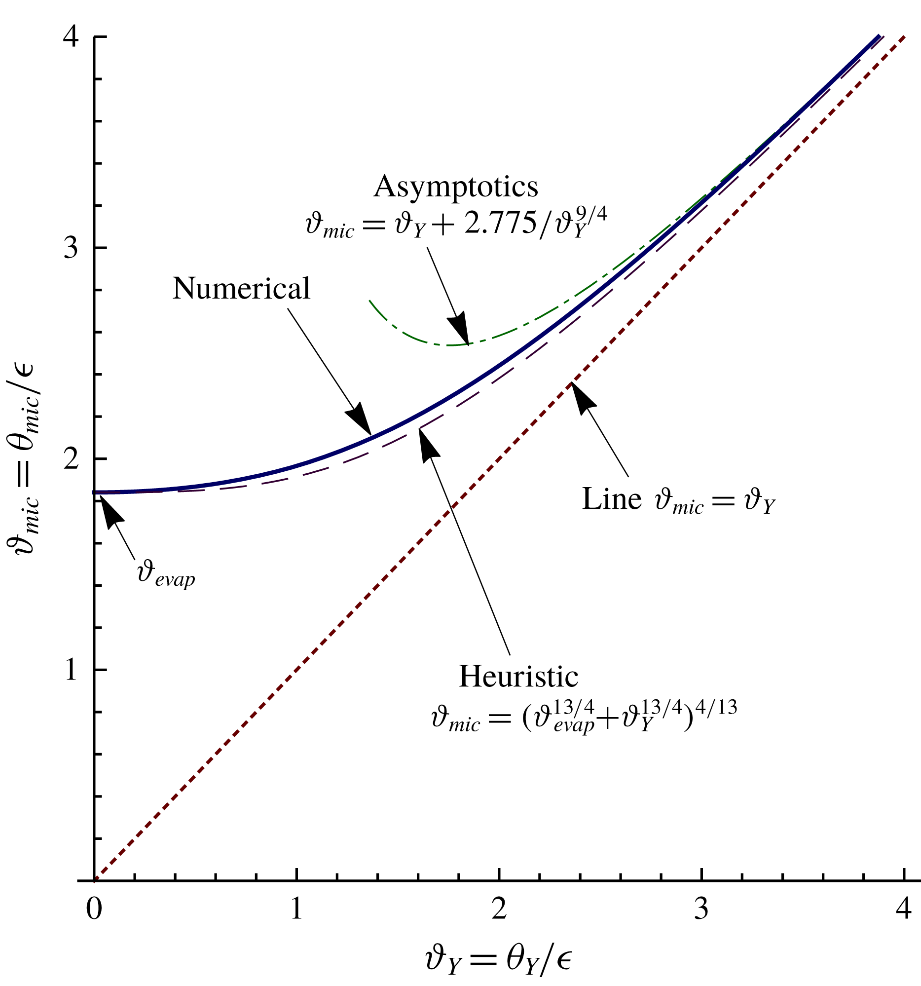
Microregion contact angle versus Young’s angle (both rescaled with
 $\unicode[STIX]{x1D716}$
) in the purely evaporative case (case I of table 1). The part
 $(\unicode[STIX]{x1D717}_{mic}-\unicode[STIX]{x1D717}_{Y})$
of
 $\unicode[STIX]{x1D717}_{mic}$
is evaporation induced.
Numerical results for the angle
 $\unicode[STIX]{x1D717}_{mic}$
as a function of
 $\unicode[STIX]{x1D717}_{Y}$
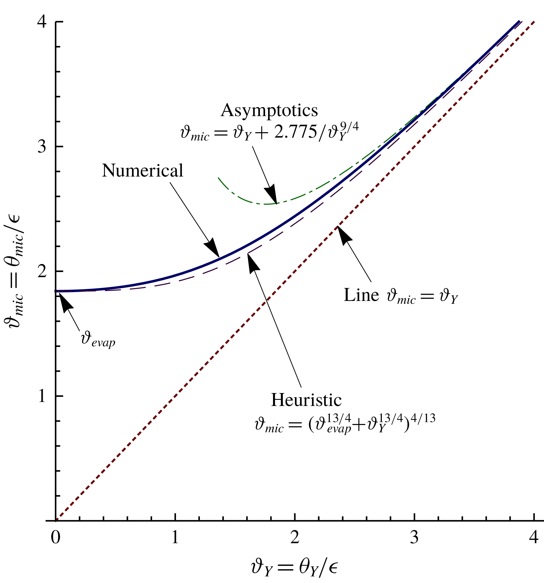
are represented by a solid line in figure 3. As can be expected,
 $\unicode[STIX]{x1D717}_{mic}$
always exceeds
 $\unicode[STIX]{x1D717}_{Y}$
due to an evaporation-induced contribution. Most remarkably, we have a finite microregion angle
 $\unicode[STIX]{x1D717}_{mic}$
in the perfect-wetting case
 $\unicode[STIX]{x1D717}_{Y}=0$
, when
 $\unicode[STIX]{x1D717}_{mic}$
is totally due to evaporation. This constitutes the evaporation-induced contact angle
 $$\begin{eqnarray}\unicode[STIX]{x1D717}_{evap}\equiv \unicode[STIX]{x1D717}_{mic}|_{\unicode[STIX]{x1D717}_{Y}=0}\approx 1.841\quad (\unicode[STIX]{x1D703}_{evap}\equiv \unicode[STIX]{x1D703}_{mic}|_{\unicode[STIX]{x1D703}_{Y}=0}\approx 1.841\,\unicode[STIX]{x1D716}),\end{eqnarray}$$
where recall that
 $\unicode[STIX]{x1D716}$
given by (4.2) with (2.21). On the other hand, also quite expectedly, the evaporation-induced part, (
 $\unicode[STIX]{x1D717}_{mic}-\unicode[STIX]{x1D717}_{Y}$
), becomes decreasingly important against
 $\unicode[STIX]{x1D717}_{Y}$
as the latter is increased. What may be less expected is that (
 $\unicode[STIX]{x1D717}_{mic}-\unicode[STIX]{x1D717}_{Y}$
) thereby decreases not only relative to
 $\unicode[STIX]{x1D717}_{Y}$
, but also in absolute value. This is confirmed by the asymptotic behaviour at
 $\unicode[STIX]{x1D717}_{Y}\gg 1$
shown in figure 3 as well (see § 4.2 for further details). We shall here also test the following correlation, whose form is inspired by the Cox–Voinov cubic power law known for the motion-induced apparent contact angles, while the power
 $13/4$
(instead of the cubic one) is chosen to recover the asymptotic form at
 $\unicode[STIX]{x1D717}_{Y}\gg 1$
displayed in figure 3:
 $\unicode[STIX]{x1D717}_{mic}^{13/4}=\unicode[STIX]{x1D717}_{evap}^{13/4}+\unicode[STIX]{x1D717}_{Y}^{13/4}$
(or rather
 $\unicode[STIX]{x1D703}_{mic}^{13/4}=\unicode[STIX]{x1D703}_{evap}^{13/4}+\unicode[STIX]{x1D703}_{Y}^{13/4}$
). It is seen to work fairly well and may be used for practical estimations.
With an estimation
 $\unicode[STIX]{x1D716}\sim 0.1$
(see the paragraph below (4.2)), the evaporation-induced angle
 $\unicode[STIX]{x1D703}_{evap}=1.841\,\unicode[STIX]{x1D716}$
expressed in degrees is of the order of
 $\unicode[STIX]{x1D703}_{evap}\sim 11^{\circ }$
. More concrete estimations of the Kelvin-only values of
 $\unicode[STIX]{x1D703}_{evap}$
for a number of liquids are provided in appendix B and table 2.
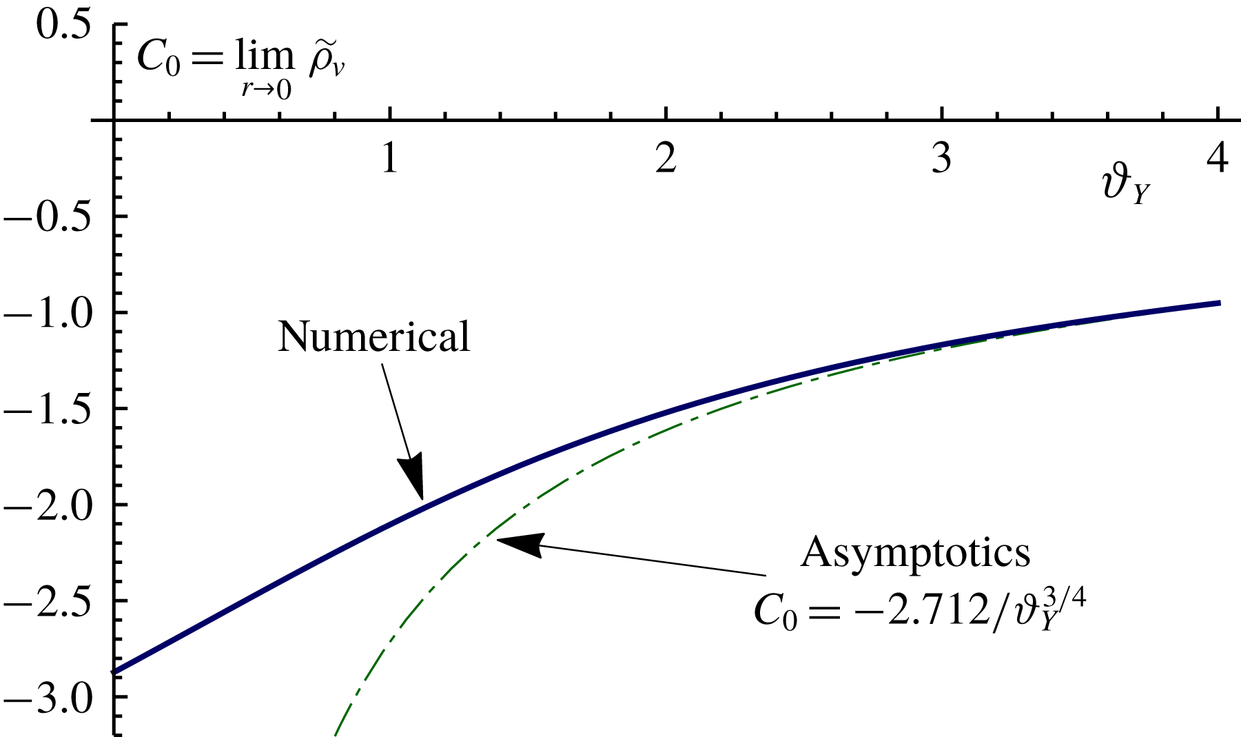
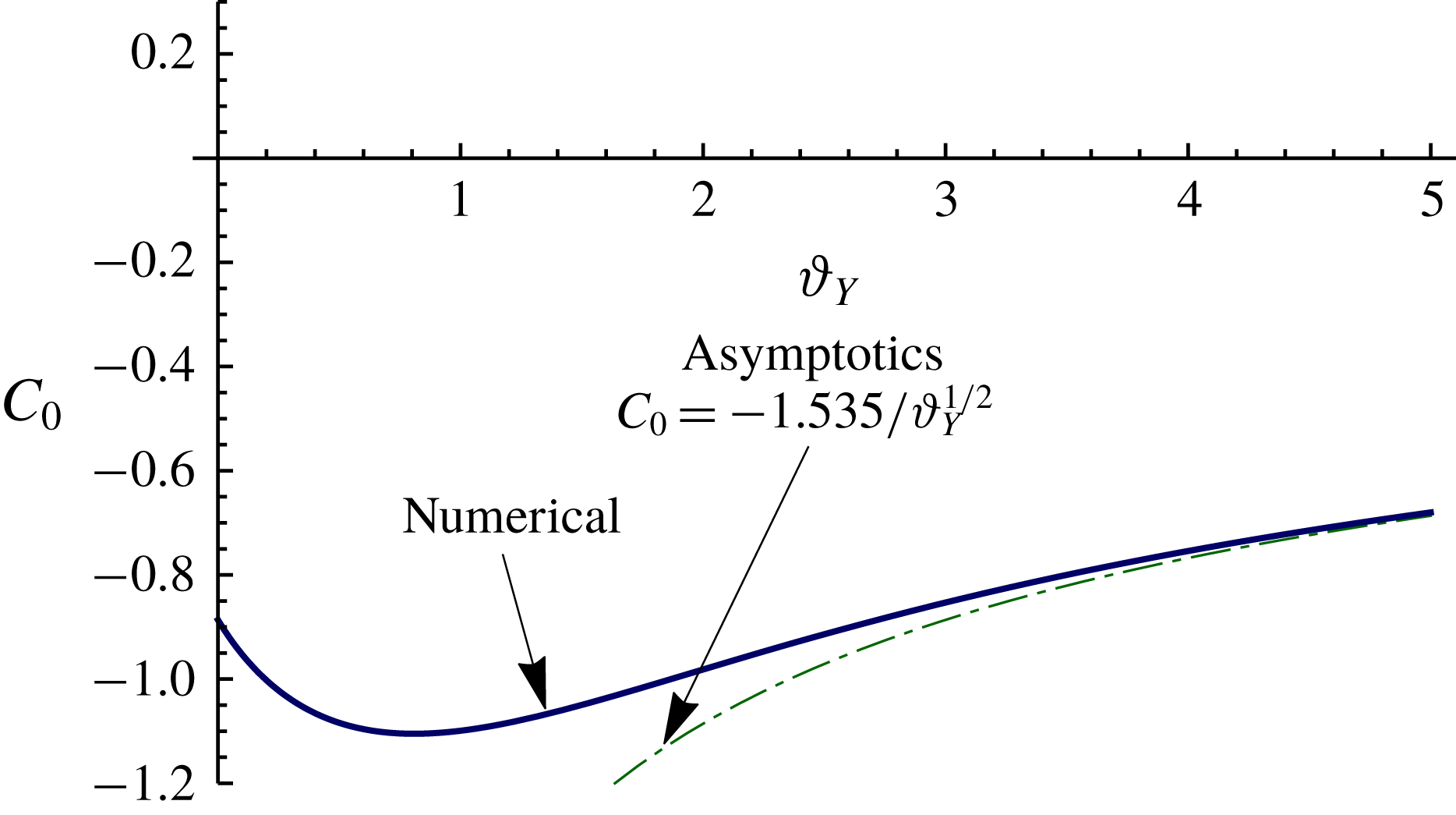
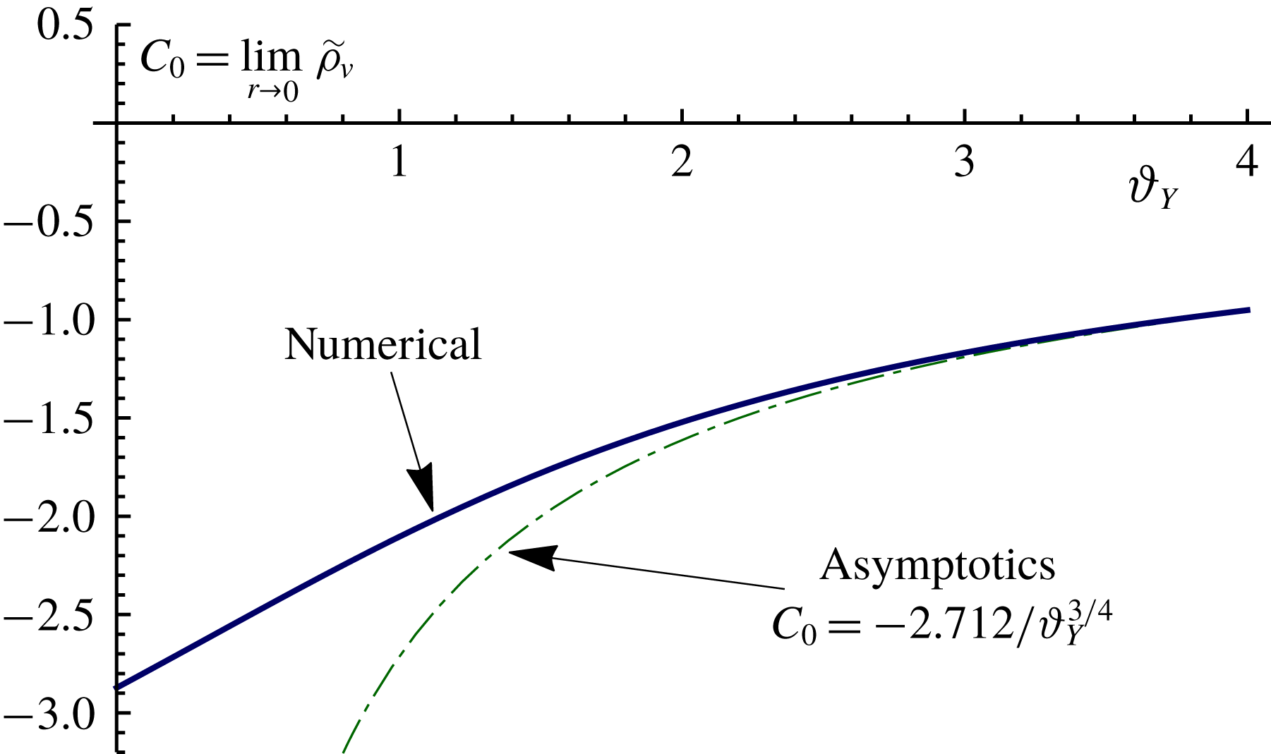
The Kelvin effect in our system is quantitatively characterised in figure 4, where the dimensionless deviation of the actual vapour density at the tip of the film from the flat-interface saturation vapour density is shown as a function of the rescaled Young’s angle. Up to a factor of
 $(-3)$
, this is equal to the corresponding dimensionless film curvature. The asymptotic behaviour at
 $\unicode[STIX]{x1D717}_{Y}\gg 1$
(see § 4.2) is displayed as well.
Dimensionless vapour-density deviation at the film tip
 $\tilde{\unicode[STIX]{x1D70C}}_{v}|_{r=0}=C_{0}$
(cf. (4.5)) versus the rescaled Young’s angle
 $\unicode[STIX]{x1D717}_{Y}=\unicode[STIX]{x1D703}_{Y}/\unicode[STIX]{x1D716}$
. It is related to the dimensionless film curvature as
 $\tilde{\unicode[STIX]{x1D70C}}_{v}|_{r=0}=C_{0}=-3\,\text{d}^{2}h/\text{d}x^{2}|_{x=0}$
due to the Kelvin effect (cf. (2.16b
)). Purely evaporative case (case I of table 1).
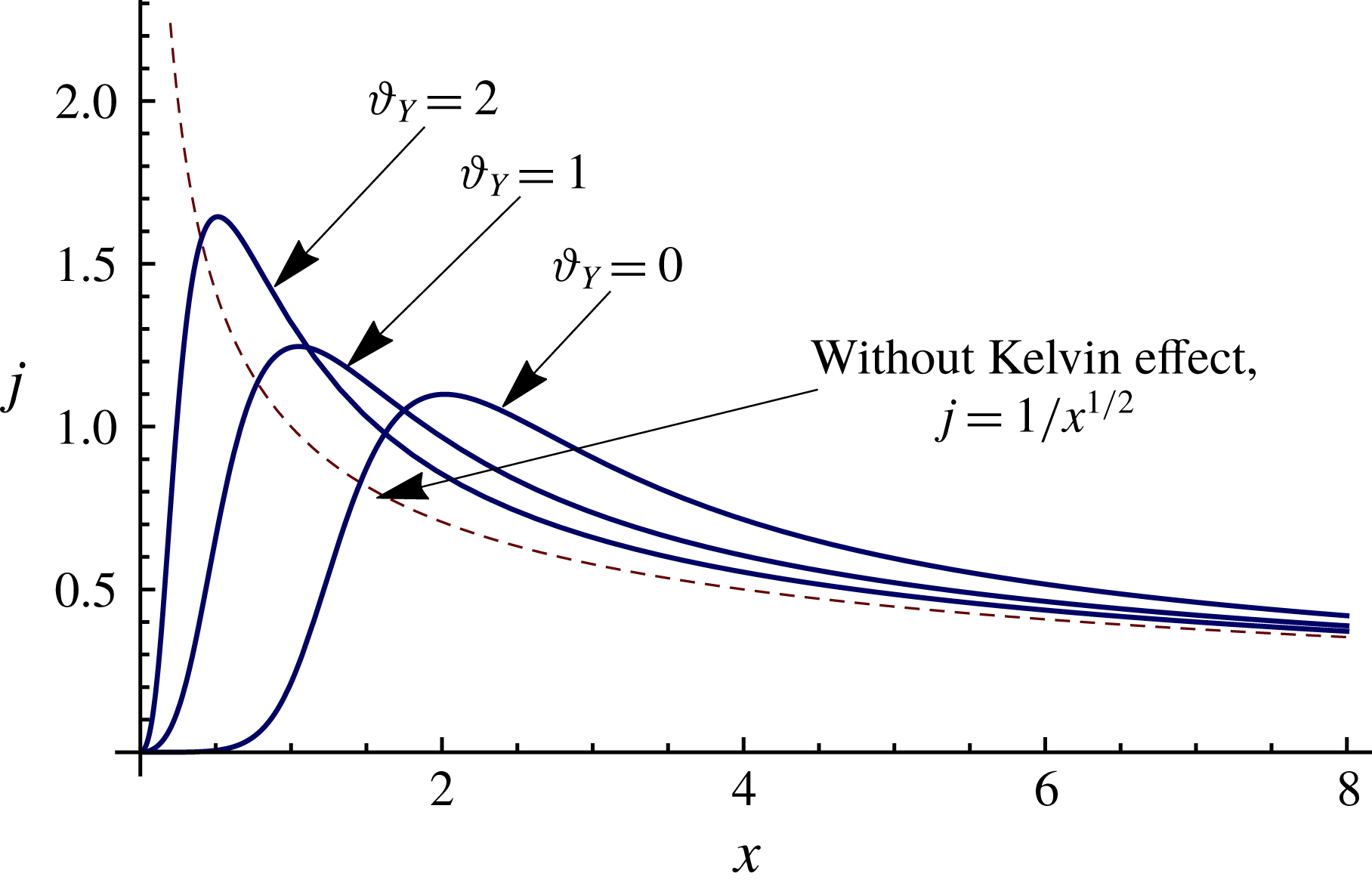
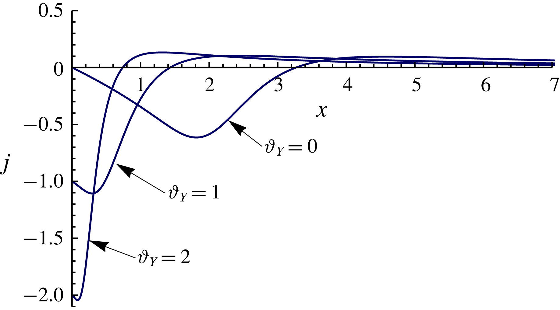
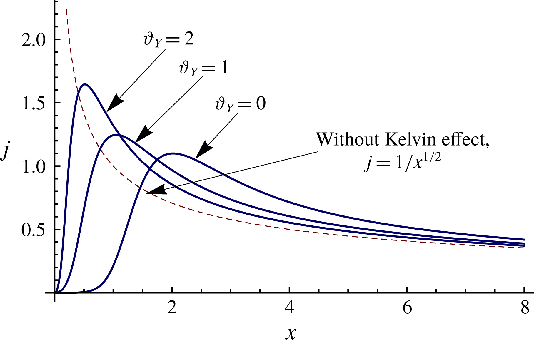
Finally, figure 5 shows the local evaporation rate distribution along the film for a number of
 $\unicode[STIX]{x1D717}_{Y}$
values. As already mentioned, a noteworthy feature is the regularisation of the flux at small
 $x$
by the Kelvin effect, whereas at large
 $x$
the flux still attains its form
 $j=1/x^{1/2}$
in the absence of the Kelvin effect. Interestingly, in spite of the regularisation, the integral flux does not change:
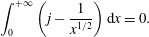 $$\begin{eqnarray}\int _{0}^{+\infty }\left(j-\frac{1}{x^{1/2}}\right)\text{d}x=0.\end{eqnarray}$$
Indeed, we have
 $\int _{0}^{\unicode[STIX]{x03C0}}\unicode[STIX]{x2202}(\tilde{\unicode[STIX]{x1D70C}}_{v}+2r^{1/2}\sin \unicode[STIX]{x1D711}/2)/\unicode[STIX]{x2202}r\;r\,\text{d}\unicode[STIX]{x1D711}\rightarrow 0$
as
 $r\rightarrow +\infty$
, which can be established with the help of the coordinate expansion (C 2). In other words, the difference of the diffusion fluxes, in the presence and in the absence of the Kelvin effect, through an infinite semicircle about the contact line vanishes. Equation (4.7) then follows from the species conservation.
Dimensionless local evaporation rate profiles in the contact-line microregion for a number of values of the rescaled Young’s angle
 $\unicode[STIX]{x1D717}_{Y}=\unicode[STIX]{x1D703}_{Y}/\unicode[STIX]{x1D716}$
. Purely evaporative case (case I of table 1). Numerical results (solid lines). In the absence of the Kelvin effect, the result would universally be given by the dashed line.
In the context of an asymptotic analysis of an evaporating sessile drop (Saxton et al.
Reference Saxton, Whiteley, Vella and Oliver2016; Savva et al.
Reference Savva, Rednikov and Colinet2017), note that it is
 $\unicode[STIX]{x1D717}_{mic}$
(or
 $\unicode[STIX]{x1D703}_{mic}$
) that directly occurs as the apparent contact angle at the slow evaporation (mass loss) stage of drop evolution. Furthermore, at a faster, initial spreading/retraction stage, it is this angle that serves as the microscopic angle input in the Cox–Voinov law (Saxton et al.
Reference Saxton, Whiteley, Vella and Oliver2016; Savva et al.
Reference Savva, Rednikov and Colinet2017). The latter situation will be the subject of § 4.3 later on.
4.2 Weak phase-change limit (evaporation or condensation) for a finite Young’s angle (case II)
We still remain in the framework of the purely evaporative case of § 4.1 (with
 $c=0$
). We now ask ourselves what happens in the limit of weak evaporation and even whether such a limit makes sense at all. Obviously, it does not make much sense in the situation of perfect wetting, with a vanishing Young’s angle (
 $\unicode[STIX]{x1D703}_{Y}=\unicode[STIX]{x1D717}_{Y}=0$
). Indeed, the scale (4.2) of the evaporation-induced angles has then nothing to be considered small against however small the evaporation driving factor
 $(\unicode[STIX]{x1D70C}_{v,sat}^{\ast }-\unicode[STIX]{x1D70C}_{v,\infty }^{\ast })$
may actually be made. On the contrary, it makes perfect sense for partial wetting and finite Young’s angles, against which the evaporation-induced angles can now be considered small. The weak evaporation limit should then correspond to the latter being much smaller than the former, i.e. to
 $\unicode[STIX]{x1D716}\ll \unicode[STIX]{x1D703}_{Y}$
with
 $\unicode[STIX]{x1D716}$
defined in (4.2). On account of the angle rescaling (2.23), this can be rewritten as
 $$\begin{eqnarray}\unicode[STIX]{x1D717}_{Y}\gg 1\quad (\text{scaling}~{\mathcal{K}}\equiv 1,\,E\equiv 1),\end{eqnarray}$$
and the limit of weak evaporation is thereby equivalent to the limit of large rescaled Young’s angles in the considered scaling. The present subsection is thus dedicated to this important limiting case of § 4.1, referred to as case II in table 1. Note that the present notion of a weak evaporation limit is the same as invoked elsewhere (cf. e.g. Savva et al. Reference Savva, Rednikov and Colinet2017).
However, when considering the limit in question, it appears to be more natural to proceed in terms of a scaling based on the largest of the angle contributions involved, i.e. on Young’s angle, and not on the evaporation-induced ones as in § 4.1 (the principle of dominant balance). Specifically, we can work in terms of the scaling
 $\unicode[STIX]{x1D717}_{Y}\equiv 1$
, which in accordance with (2.23a
) now implies the choice
 $$\begin{eqnarray}\unicode[STIX]{x1D716}=\unicode[STIX]{x1D703}_{Y}\quad (\text{scaling}~{\mathcal{K}}\equiv 1,\,\unicode[STIX]{x1D717}_{Y}\equiv 1),\end{eqnarray}$$
in lieu of (4.2). Recall that all the angles and film slopes are assumed small in the present paper, and hence
 $\unicode[STIX]{x1D716}\ll 1$
here relies upon
 $\unicode[STIX]{x1D703}_{Y}\ll 1$
. Recall also that the dimensionless numbers, angle rescalings and dimensional scales of the problem are generically given by (2.20)–(2.24), now just with
 $\unicode[STIX]{x1D716}$
defined by (4.9). This gives rise to the ensemble of microregion scales determined by the Kelvin effect and Young’s angle.
In terms of this new scaling, the weak evaporation condition (4.8) rather adopts a more natural form
 $$\begin{eqnarray}E\ll 1\quad (\text{scaling}~{\mathcal{K}}\equiv 1,\,\unicode[STIX]{x1D717}_{Y}\equiv 1),\end{eqnarray}$$
i.e. explicitly that of a limit of small evaporation numbers. Assuming regular perturbations, we write
 $$\begin{eqnarray}\unicode[STIX]{x1D717}_{mic}=1+\unicode[STIX]{x1D6FC}E,\quad h=x+Eh_{1}+\cdots ,\quad \tilde{\unicode[STIX]{x1D70C}}_{v}=E\tilde{\unicode[STIX]{x1D70C}}_{v1}+\cdots ,\quad j=Ej_{1}+\cdots ,\end{eqnarray}$$
where the leading-order,
 $O(E^{0})$
, result is merely given by Young’s angle throughout, whereas the evaporative effects first appear at the order
 $O(E)$
. Substituting (4.11) into (2.12) and (2.13) with
 $c=0$
and
 $\unicode[STIX]{x1D717}_{Y}\equiv 1$
as well as into (4.3) and (2.18), we obtain
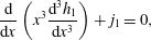 $$\begin{eqnarray}\frac{\text{d}}{\text{d}x}\left(x^{3}\frac{\text{d}^{3}h_{1}}{\text{d}x^{3}}\right)+j_{1}=0,\end{eqnarray}$$
 $$\begin{eqnarray}h_{1}=0,\quad \text{d}h_{1}/\text{d}x=0\quad \text{at}~x=0,\end{eqnarray}$$
 $$\begin{eqnarray}\displaystyle & h_{1}\sim \unicode[STIX]{x1D6FC}x\quad \text{as}~x\rightarrow +\infty , & \displaystyle\end{eqnarray}$$
 $$\begin{eqnarray}\displaystyle & \displaystyle \tilde{\unicode[STIX]{x1D70C}}_{v1}\sim -2r^{1/2}\sin \frac{\unicode[STIX]{x1D711}}{2}\quad \text{as}~r\rightarrow +\infty \quad (0\leqslant \unicode[STIX]{x1D711}\leqslant \unicode[STIX]{x03C0}). & \displaystyle\end{eqnarray}$$
Thus, the boundary-value problem for the evaporative perturbation
 $h_{1}$
,
 $\unicode[STIX]{x1D70C}_{v1}$
and
 $j_{1}$
is given by (4.12)–(4.15) that must be supplemented by equations and boundary conditions coming from the yet unused part of the original formulation. The latter part is given by (2.15)–(2.17) and (2.19) with
 ${\mathcal{K}}\equiv 1$
, in which a subscript ‘1’ must yet be appended to the dependent variables. We note that
 $\unicode[STIX]{x1D6FC}$
is a free coefficient to be determined together with the solution of the problem.
The formulated boundary-value problem contains no input parameters and is linear. The numerical treatment is similar to § 4.1, including the use of coordinate expansions. (The coordinate expansions at zero and at infinity can here be developed similarly to (4.4), (4.5), (C 1) and (C 2), and are not explicitly provided for the sake of brevity. On the other hand, they can be deduced directly from (4.4), (4.5), (C 1) and (C 2) by taking the limit (4.8) and recasting the result in term of the scaling
 ${\mathcal{K}}\equiv 1$
and
 $\unicode[STIX]{x1D717}_{Y}\equiv 1$
in lieu of
 ${\mathcal{K}}\equiv 1$
and
 $E\equiv 1$
.) The resulting linear system of equations for the values of the dependent variables at the grid points and the coefficients of the coordinate expansions is solved with the help of the NSolve command in Mathematica®.
We shall be mainly concerned with the microregion contact angle, for which the relevant numerical result is
 $$\begin{eqnarray}\unicode[STIX]{x1D6FC}=2.775.\end{eqnarray}$$
It can now be used in the first equation (4.11a
) to yield the principal result of the present subsection. Remarkably, as already anticipated in § 3, this perturbation result must be valid not only for global evaporation (
 $\unicode[STIX]{x1D70C}_{v,sat}^{\ast }>\unicode[STIX]{x1D70C}_{v,\infty }^{\ast }$
,
 $E>0$
), but also equally well for global condensation (
 $\unicode[STIX]{x1D70C}_{v,sat}^{\ast }<\unicode[STIX]{x1D70C}_{v,\infty }^{\ast }$
,
 $E<0$
). In this sense, the present case II is actually not merely a limit of case I (the latter restricted to global evaporation), but also offers an extension into the condensation domain. That is why the title of the present subsection refers to a weak phase-change limit, and not merely to a weak evaporation limit.
On the other hand, now referring specifically to a weak evaporation limit, this principal result is to be converted into the scaling
 ${\mathcal{K}}\equiv 1$
,
 $E\equiv 1$
used in § 4.1 in order to facilitate a direct comparison to case I. We obtain
 $\unicode[STIX]{x1D717}_{mic}=\unicode[STIX]{x1D717}_{Y}+2.775\,\unicode[STIX]{x1D717}_{Y}^{-9/4}$
, which, in accordance with its applicability (4.8), serves as a large Young’s angle asymptotic for
 $\unicode[STIX]{x1D717}_{mic}$
in figure 3, as already mentioned in § 4.1.
Finally, we also note another result of the computation carried out in the weak phase-change limit. Namely,
 $\tilde{\unicode[STIX]{x1D70C}}_{v1}|_{r=0}=-2.712$
. On account of (4.11c
), this yields
 $\tilde{\unicode[STIX]{x1D70C}}_{v}|_{r=0}=-2.712E$
at
 $E\ll 1$
in the scaling
 ${\mathcal{K}}\equiv 1$
,
 $\unicode[STIX]{x1D717}_{Y}\equiv 1$
. If rather rewritten in the scaling
 ${\mathcal{K}}\equiv 1$
,
 $E\equiv 1$
, it becomes
 $\tilde{\unicode[STIX]{x1D70C}}_{v}|_{r=0}=-2.712\,\unicode[STIX]{x1D717}_{Y}^{-3/4}$
at
 $\unicode[STIX]{x1D717}_{Y}\gg 1$
represented in figure 4 as the corresponding asymptotic behaviour.
4.3 Accounting for contact-line motion in the general case (case III)
Here we consider a case of a moving contact line (
 $c\neq 0$
) and show that the moving contact-line singularity, too, can be handled solely thanks to the Kelvin effect.
As already mentioned, it is now our angle
 $\unicode[STIX]{x1D703}_{mic}$
that is expected to appear at the microscopic angle entering the Cox–Voinov relation (viscous bending) defined in an intermediate region of a moving contact line, between the microregion and the macroscopic one. We shall verify later on that this is indeed the case. The relation in question can then be represented as (see e.g. Bonn et al.
Reference Bonn, Eggers, Indekeu, Meunier and Rolley2009)
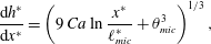 $$\begin{eqnarray}\frac{\text{d}h^{\ast }}{\text{d}x^{\ast }}=\left(9\,Ca\ln \frac{x^{\ast }}{\ell _{mic}^{\ast }}+\unicode[STIX]{x1D703}_{mic}^{3}\right)^{1/3},\end{eqnarray}$$
valid at sufficiently large
 $x^{\ast }/\ell _{mic}^{\ast }$
. The parameter here denoted as
 $\ell _{mic}^{\ast }$
represents the Voinov (micro)length. In terms of our dimensionless variables (cf. (2.20), (2.22) and (2.23)), this can be rewritten as
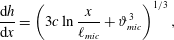 $$\begin{eqnarray}\frac{\text{d}h}{\text{d}x}=\left(3c\ln \frac{x}{\ell _{mic}}+\unicode[STIX]{x1D717}_{mic}^{3}\right)^{1/3},\end{eqnarray}$$
valid at sufficiently large
 $x$
. Here
 $$\begin{eqnarray}\ell _{mic}=\ell _{mic}^{\ast }/[x],\end{eqnarray}$$
which is made dimensionless with the microregion length scale
 $[x]$
. It is generally expected that
 $\ell _{mic}=O(1)$
, in the same way as
 $\unicode[STIX]{x1D717}_{mic}=O(1)$
. One can verify that (4.18) represents indeed the asymptotic behaviour at sufficiently large distances within our film equation (2.12) with
 $c\neq 0$
, satisfying (2.14), given that
 $j$
decays fast enough (as
 $j\sim x^{-1/2}$
, in accordance with (2.18) and (2.16a
)). (In contrast,
 $j$
does not decay in the cases studied by Hocking (Reference Hocking1995) and Oliver et al. (Reference Oliver, Whiteley, Saxton, Vella, Zubkov and King2015), where the Cox–Voinov law is not valid in this form.) The behaviour (4.18) is to be matched with the solution in the macroscopic region. This yields in particular the angle as apparent at macroscopic scales, which can be written as
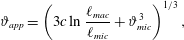 $$\begin{eqnarray}\unicode[STIX]{x1D717}_{app}=\left(3c\ln \frac{\ell _{mac}}{\ell _{mic}}+\unicode[STIX]{x1D717}_{mic}^{3}\right)^{1/3},\end{eqnarray}$$
where
 $\ell _{mac}$
is an appropriate macroscopic length (
 $\ell _{mac}\gg 1$
as it is here represented in microregion units
 $[x]$
). For instance, for a spreading/retracting sessile drop of a radius
 $R_{c}$
, the spherical-cap apparent contact angle corresponds to
 $l_{mac}=R_{c}/(2e^{2})$
(e.g. Hocking Reference Hocking1983; Bonn et al.
Reference Bonn, Eggers, Indekeu, Meunier and Rolley2009; Savva et al.
Reference Savva, Rednikov and Colinet2017), this result not being affected by the phase change within the asymptotic scheme by Saxton et al. (Reference Saxton, Whiteley, Vella and Oliver2016) and Savva et al. (Reference Savva, Rednikov and Colinet2017).
The logarithm values in (4.17)–(4.20) are inherently large. Consider a distinguished asymptotic limit when the slopes and apparent contact angles deviate from the microscopic angle by the order of themselves. One can then see, from (4.18) and (4.20), that this corresponds in fact to
 $c\ll 1$
in a scaling where
 $\unicode[STIX]{x1D717}_{mic}=O(1)$
, whilst
 $c\ln \ell _{mac}/\ell _{mic}=O(1)$
. This is the asymptotic case we shall be interested in the present subsection.
Thus, it is essentially a question of considering an
 $O(c)$
correction upon the results of case I developed in § 4.1. It will be appropriate to proceed in the same scaling as in § 4.1, i.e.
 ${\mathcal{K}}\equiv 1$
,
 $E\equiv 1$
. The case studied in the present subsection can symbolically be designated as
 $$\begin{eqnarray}c\ll 1\quad (\text{scaling}~{\mathcal{K}}\equiv 1,\,E\equiv 1),\end{eqnarray}$$
which corresponds to case III in table 1. As anticipated in § 3, such a perturbation analysis will be valid for both advancing (
 $c>0$
) and receding (
 $c<0$
) contact lines.
The solution is sought in the form
 $$\begin{eqnarray}h=h_{0}+ch_{1}+\cdots ,\quad \tilde{\unicode[STIX]{x1D70C}}_{v}=\tilde{\unicode[STIX]{x1D70C}}_{v0}+c\tilde{\unicode[STIX]{x1D70C}}_{v1}+\cdots ,\quad j=j_{0}+cj_{1}+\cdots .\end{eqnarray}$$
In the present subsection, the subscript ‘0’ marks the solution obtained in § 4.1 for case I (
 $c=0$
) and here considered known for any given
 $\unicode[STIX]{x1D717}_{Y}$
, while the subscript ‘1’ refers to the motion-induced correction to be determined.
Using (4.21) and (4.22) in the system (2.12)–(2.19), we obtain the following problem for the correction:
 $$\begin{eqnarray}\frac{\text{d}h_{0}}{\text{d}x}+\frac{\text{d}}{\text{d}x}\left(h_{0}^{3}\frac{\text{d}^{3}h_{1}}{\text{d}x^{3}}\right)+3\frac{\text{d}}{\text{d}x}\left(h_{0}^{2}h_{1}\frac{\text{d}^{3}h_{0}}{\text{d}x^{3}}\right)+j_{1}=0\quad (x>0),\end{eqnarray}$$
 $$\begin{eqnarray}h_{1}=0,\quad \text{d}h_{1}/\text{d}x=0\quad \text{at}~x=0,\end{eqnarray}$$
 $$\begin{eqnarray}\tilde{\unicode[STIX]{x1D70C}}_{v1}/r^{1/2}\rightarrow 0\quad \text{as}~r\rightarrow +\infty \quad (0\leqslant \unicode[STIX]{x1D711}\leqslant \unicode[STIX]{x03C0}),\end{eqnarray}$$
while (2.14)–(2.17) and (2.19) remain exactly the same in terms of the corrections (provided that the dependent variables take an additional subscript ‘1’ and
 ${\mathcal{K}}\equiv 1$
) and are not rewritten here for the sake of brevity. This completes the formulation of the boundary-value problem for
 $h_{1}$
,
 $\tilde{\unicode[STIX]{x1D70C}}_{v1}$
and
 $j_{1}$
.
Remarkably, as in § 4.1, we are able to find a non-singular behaviour at the tip of the film compatible with the given formulation, signifying a successful resolution thanks to the Kelvin effect, this time, of the moving contact-line singularity:
 $$\begin{eqnarray}h_{1}\sim -\frac{1}{6}C_{01}x^{2}-\frac{\unicode[STIX]{x1D717}_{Y}}{18\unicode[STIX]{x03C0}}x^{3}\ln x+\frac{5\unicode[STIX]{x1D717}_{Y}-6\unicode[STIX]{x03C0}C_{11}}{108\unicode[STIX]{x03C0}}x^{3}+\cdots \quad \text{as}~x\rightarrow 0\end{eqnarray}$$
and
 $$\begin{eqnarray}\displaystyle \tilde{\unicode[STIX]{x1D70C}}_{v1} & {\sim} & \displaystyle C_{01}+\frac{\unicode[STIX]{x1D717}_{Y}}{\unicode[STIX]{x03C0}}r[\ln r\cos \unicode[STIX]{x1D711}-(\unicode[STIX]{x1D711}-\unicode[STIX]{x03C0})\sin \unicode[STIX]{x1D711}]+C_{11}r\cos \unicode[STIX]{x1D711}\nonumber\\ \displaystyle & & \displaystyle -\,\frac{C_{00}}{6\unicode[STIX]{x03C0}}r^{2}[\ln r\cos 2\unicode[STIX]{x1D711}-(\unicode[STIX]{x1D711}-\unicode[STIX]{x03C0})\sin 2\unicode[STIX]{x1D711}]+C_{21}r^{2}\cos 2\unicode[STIX]{x1D711}+\cdots \quad \text{as}~r\rightarrow 0.\qquad\end{eqnarray}$$
Here, in the spirit of the ‘0-subscript convention’ made above,
 $C_{00}$
stands for
 $C_{0}$
of § 4.1 (
 $C_{00}$
being considered known for any given
 $\unicode[STIX]{x1D717}_{Y}$
from § 4.1), whereas
 $C_{01}$
,
 $C_{11}$
and
 $C_{21}$
are new free coefficients to be determined together with the solution of the present subsection. Note that, in the presence of contact-line motion, the coordinate expansions have here become somewhat more singular than before, with
 $\unicode[STIX]{x2202}\tilde{\unicode[STIX]{x1D70C}}_{v}/\unicode[STIX]{x2202}r$
and
 $\text{d}^{3}h_{1}/\text{d}x^{3}$
diverging logarithmically as
 $r\rightarrow 0$
and
 $x\rightarrow 0$
. Yet this is still sufficient for being considered a singularity-free behaviour. In particular, the shear stress (2.25) still vanishes towards the contact line (
 $x\rightarrow 0$
) as
 $\unicode[STIX]{x1D70E}_{\unicode[STIX]{x1D70F}}\sim -(1/3)\unicode[STIX]{x03C0}^{-1}\unicode[STIX]{x1D717}_{Y}^{2}x\ln x$
so that not even a remote doubt arises about its integrability.
A key feature of this moving contact-line singularity resolution is the fact that the phase change at the tip of film self-adjusts, thanks to the Kelvin effect, to the tip motion. In other words, the tip advances (
 $c>0$
) by means of the appropriate amount of local condensation (
 $j<0$
) and recedes (
 $c<0$
) by means of the appropriate amount of local evaporation (
 $j>0$
), the actual liquid velocity vanishing at the tip in both cases (hence satisfying the no-slip condition at the substrate). Indeed, from (2.16a
), (4.5), (4.22) and (4.27), one can find
 $j_{0}=0$
,
 $j_{1}=-\unicode[STIX]{x1D717}_{Y}$
and thus
 $j=-c\unicode[STIX]{x1D717}_{Y}$
as
 $x\rightarrow 0$
, which confirms the point. Thus, kinematically, it happens here in the same way as in the case of a pure-vapour atmosphere (Rednikov & Colinet Reference Rednikov and Colinet2013), in spite of the essentially different phase-change mechanisms here and there.
For a moving contact line, it is no longer possible to end up with a constant film slope far away from the microregion as in (4.3). Rather, the slope diverges logarithmically. Indeed, the behaviour compatible with (4.23) and (2.14) can now be found as
 $$\begin{eqnarray}h_{1}\sim \frac{1}{\unicode[STIX]{x1D717}_{mic}^{2}}x\ln \frac{x}{e\ell _{mic}}+\cdots \quad \text{as}~x\rightarrow +\infty ,\end{eqnarray}$$
where
 $\ell _{mic}$
is a free coefficient to be determined with the solution of the present problem for the motion-induced correction, whereas
 $\unicode[STIX]{x1D717}_{mic}$
is considered known for any given
 $\unicode[STIX]{x1D717}_{Y}$
from the computation of case I (cf. § 4.1). We will see shortly that
 $\ell _{mic}$
is here actually the same quantity as in (4.18). On account of (4.25), the leading-order behaviour at infinity for the concentration field and mass flux corrections can be found as
 $$\begin{eqnarray}\tilde{\unicode[STIX]{x1D70C}}_{v1}\sim \frac{B_{11}}{r^{1/2}}\sin \frac{\unicode[STIX]{x1D711}}{2}+\cdots \quad \text{as}~r\rightarrow +\infty ,\qquad j_{1}\sim -\frac{B_{11}}{2x^{3/2}}+\cdots \quad \text{as}~x\rightarrow +\infty ,\end{eqnarray}$$
where
 $B_{11}$
is yet another free coefficient to be determined with the solution. Note that unlike the leading-order behaviour (2.18) taken up by
 $\tilde{\unicode[STIX]{x1D70C}}_{v0}$
, the correction
 $\tilde{\unicode[STIX]{x1D70C}}_{v1}$
fades away at infinity. At the same time,
 $j_{1}$
decays faster than
 $j_{0}$
, namely as
 $O(x^{-3/2})$
versus
 $O(x^{-1/2})$
. Further developments of the coordinate expansions (4.28) and (4.29) can be found in appendix C.
Combining the behaviours (4.3), which should now be used for
 $h_{0}$
, and (4.28) within (4.22a
), we obtain
 $$\begin{eqnarray}h\sim \unicode[STIX]{x1D717}_{mic}x+\frac{c}{\unicode[STIX]{x1D717}_{mic}^{2}}x\ln \frac{x}{e\ell _{mic}}\quad \text{as}~x\rightarrow +\infty .\end{eqnarray}$$
We see that, in spite of
 $c\ll 1$
, for sufficiently large
 $x$
such as
 $c\ln x=O(1)$
, the result (4.30) ceases to be valid. Indeed, the correction becomes of the order of the main approximation. Then it is rather the Cox–Voinov profile (4.18) that takes over. Matching between the results (4.30) and (4.18) just confirms our anticipation that
 $\unicode[STIX]{x1D717}_{mic}$
and
 $\ell _{mic}$
are the same quantities here and there.
The numerical approach used for the present linear boundary-value problem is basically the same as in § 4.2. The numerical solution obtained is once again found to smoothly adhere to the coordinate expansions, as illustrated in figure 6. This is a numerical confirmation that the local singularity-free behaviours (4.26) and (4.27) do really occur within the overall microregion solution.
Film-slope profiles for the motion-induced correction. Case III of table 1. Numerical solution (solid lines) and the coordinate expansions (dashed lines) at small and large
 $x$
.
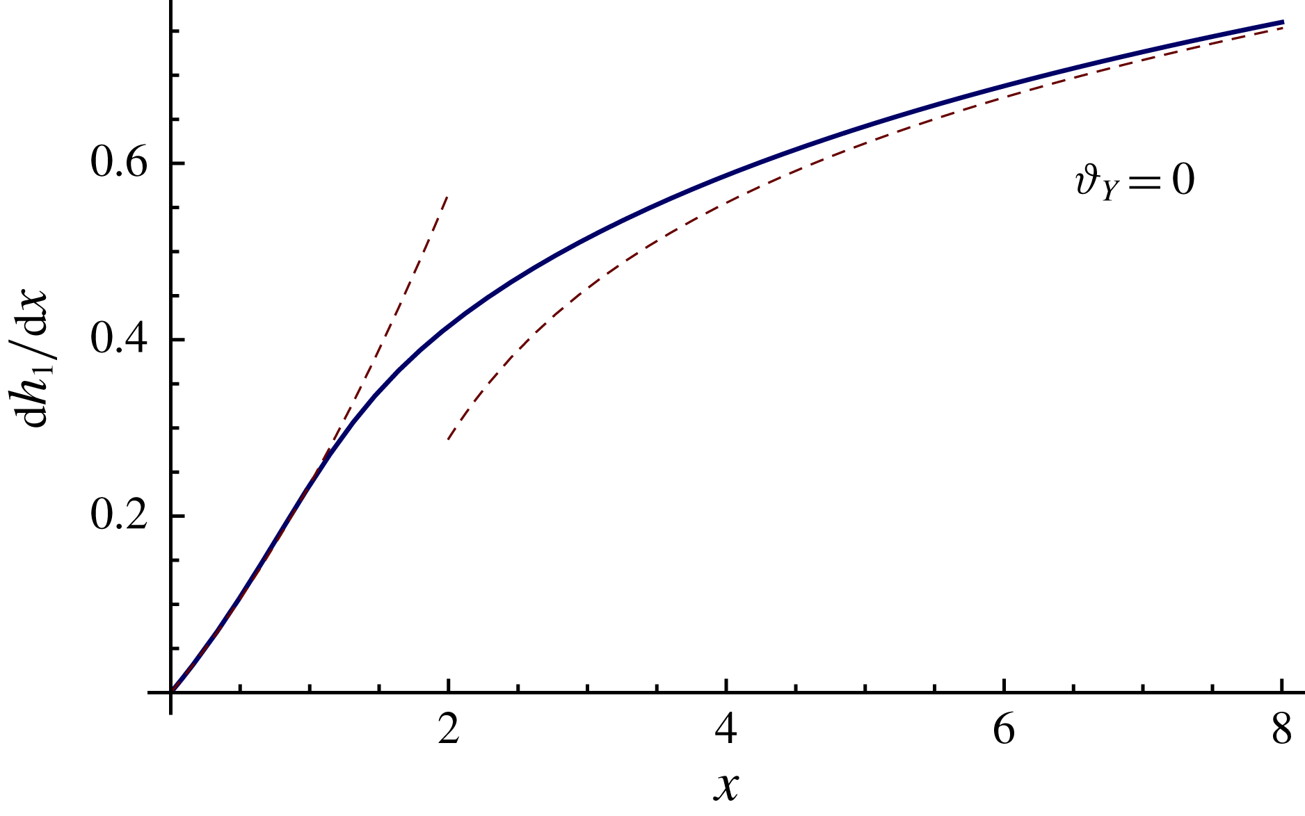
The numerical results for
 $\ell _{mic}$
as a function of
 $\unicode[STIX]{x1D717}_{Y}$
are displayed in figure 7. The strength of the induced Kelvin effect can be characterised by the vapour-density deviation at the tip of the film from its classical saturation value
 $\unicode[STIX]{x1D70C}_{v,sat}^{\ast }$
, the deviation being related to the curvature of the film. This is represented in figure 8 for the correction due to contact-line motion. The asymptotic behaviours also shown in figures 7 and 8 are discussed in § 4.4 below.
4.4 Accounting for contact-line motion for partial wetting and negligible global phase change or saturated atmosphere (case IV)
In the present subsection, we deal with a situation when the contact line is moving while global phase change is negligible. What makes such a situation of special interest is that this permits observing moving contact-line singularity resolution in its pure form, without the evaporative one getting in the way as in case III of § 4.3. In spite of the implied absence of global phase change, the local one induced by the Kelvin effect within the microregion must still be essential for the singularity resolution.
Dimensionless (scale
 $[x]$
) Voinov microlength versus the rescaled Young’s angle
 $\unicode[STIX]{x1D717}_{Y}=\unicode[STIX]{x1D703}_{Y}/\unicode[STIX]{x1D716}$
in the case when contact-line motion is a perturbation in the microregion (case III of table 1), cf. (4.18) where
 $\unicode[STIX]{x1D717}_{mic}$
is as given by figure 3.
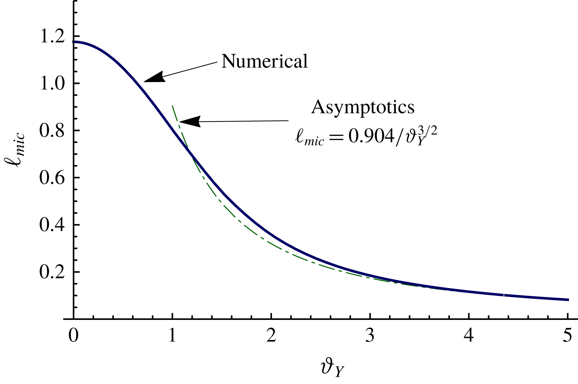


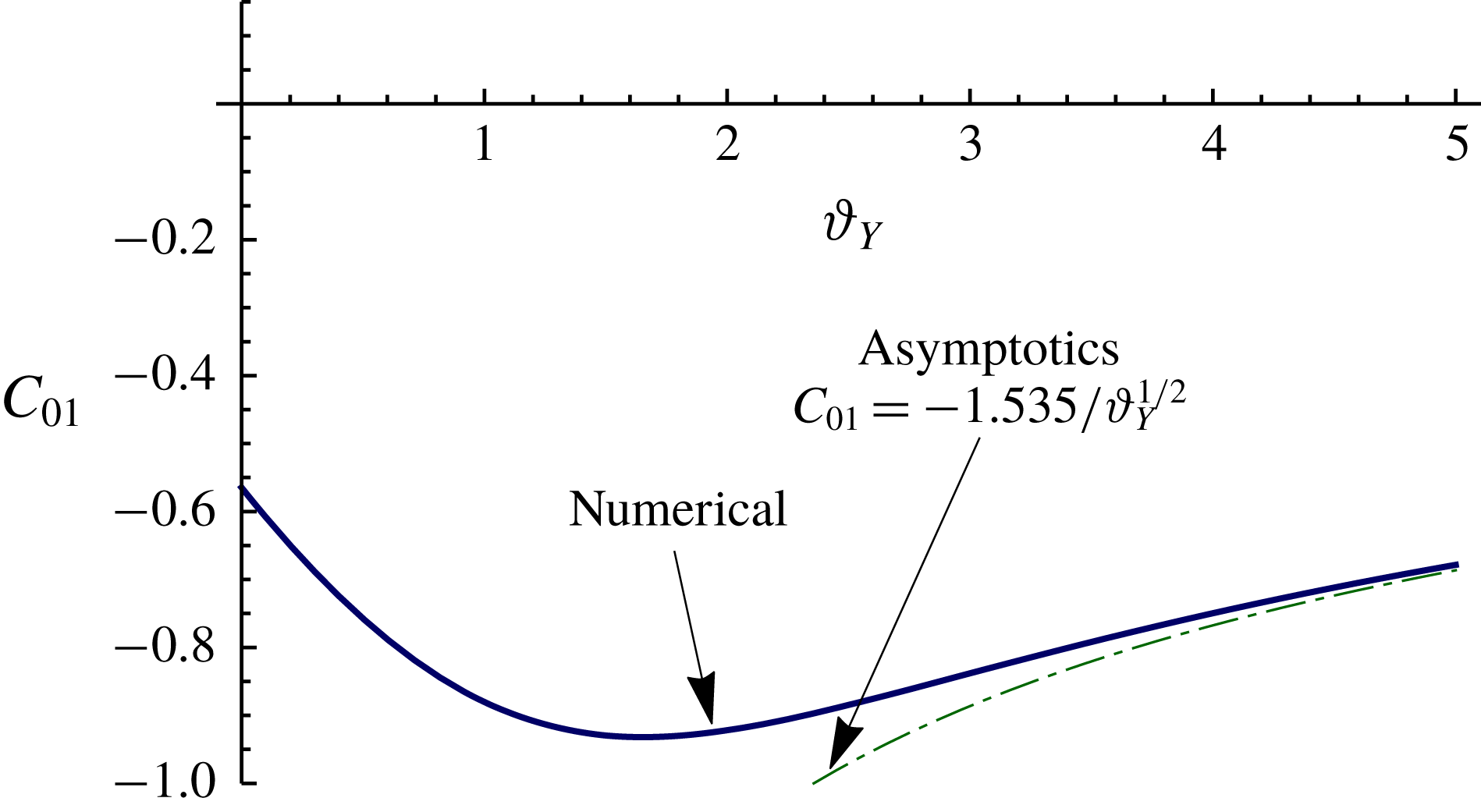
Nonetheless, a general treatment of this situation, albeit for advancing contact lines only, is relegated to § 4.5 (case V of table 1). In the present subsection, we shall rather restrict ourselves to relatively small contact-line velocities, when contact-line motion is just a perturbation, quite similar to case III considered in § 4.3 above. Such a perturbation treatment will be valid for both advancing (
 $c>0$
) and receding (
 $c<0$
) contact lines. The present study case is designated as case IV in table 1. It will be a limiting case not only of the mentioned case V for advancing contact lines, but also of case III. Such a double belonging further motivates a separate treatment of case IV carried out here. Moreover, it is just this case that was considered by Janeček et al. (Reference Janeček, Doumenc, Guerrier and Nikolayev2015).
Obviously, such a perturbation scenario here requires a finite Young’s angle and thus implies partial wetting, similar to what was outlined in the beginning of § 4.2, for otherwise there would be nothing for a perturbation to be measured against. (In contrast, in the perturbation treatment of § 4.3 (case III) perfect wetting is admissible in view of the presence of global evaporation, against which the contact-line velocity can still be considered as a perturbation in terms of the induced film slopes.) Here it is a perturbation in the sense that motion-induced film slopes remain much smaller than Young’s angle in the microregion. (Albeit not in the macroscopic region; cf. large logarithm values in the Cox–Voinov law.) As in § 4.2, the principle of dominant balance favours the scaling
 $\unicode[STIX]{x1D717}_{Y}\equiv 1$
(apart from
 ${\mathcal{K}}\equiv 1$
implied throughout). Therefore,
 $\unicode[STIX]{x1D716}$
is specified by (4.9) (i.e. simply
 $\unicode[STIX]{x1D716}=\unicode[STIX]{x1D703}_{Y}$
), with all the implications for a final specification of the dimensionless numbers and dimensional scales following then from (2.20)–(2.24). The limit of small contact-line velocities is formalised as
 $$\begin{eqnarray}c\ll 1\quad (\text{scaling}~{\mathcal{K}}\equiv 1,\,\unicode[STIX]{x1D717}_{Y}\equiv 1),\end{eqnarray}$$
which is merely equivalent to
 $Ca^{1/3}\ll \unicode[STIX]{x1D703}_{Y}$
. It is in terms of the smallness parameter (4.31) that the envisaged perturbation analysis will be carried out.
The implied absence of global phase change can be realised first of all for a saturated atmosphere (
 $\unicode[STIX]{x1D70C}_{v,\infty }^{\ast }=\unicode[STIX]{x1D70C}_{v,sat}^{\ast }$
). On the other hand, this can also be the limit of weak phase change for partial wetting, considered earlier in § 4.2: while in § 4.2 (case II) we chose to consider phase change as a perturbation for a contact line at rest, in the present subsection (case IV) we neglect it while focusing on the perturbation due to contact-line motion. Thus, we have here
 $$\begin{eqnarray}E=0.\end{eqnarray}$$
Note remarkably that the macroscopic length parameter
 $\ell ^{\ast }$
(see § 2.3) becomes then irrelevant and the present microregion problem (case IV) gets totally decoupled from the macroscopic configuration (unlike in cases I–III).
The forms of the Cox–Voinov relation (4.17)–(4.20) are still obviously valid in the context of the present case IV, albeit now specifically with
 $\unicode[STIX]{x1D703}_{mic}=\unicode[STIX]{x1D703}_{Y}$
and
 $\unicode[STIX]{x1D717}_{mic}=\unicode[STIX]{x1D717}_{Y}\equiv 1$
on account of
 $E=0$
and the scaling used. The Voinov microlength
 $\ell _{mic}$
is still a free coefficient to be determined.
The ansatz used here is quite similar to (4.11) and § 4.2 in that we proceed by looking for a perturbation solution over an equilibrium Young’s wedge:
 $$\begin{eqnarray}h=x+ch_{1}+\cdots ,\quad \tilde{\unicode[STIX]{x1D70C}}_{v}=c\tilde{\unicode[STIX]{x1D70C}}_{v1}+\cdots ,\quad j=cj_{1}+\cdots .\end{eqnarray}$$
The formulation of the problem for
 $h_{1}$
,
 $\tilde{\unicode[STIX]{x1D70C}}_{v1}$
and
 $j_{1}$
is derived upon substituting the expansions (4.33) into the general formulation (2.12)–(2.19) and retaining terms only at the order
 $O(c)$
. In particular, (2.12) thereby yields
 $$\begin{eqnarray}1+\frac{\text{d}}{\text{d}x}\left(x^{3}\frac{\text{d}^{3}h_{1}}{\text{d}x^{3}}\right)+j_{1}=0\quad (x>0),\end{eqnarray}$$
which is the case IV counterpart of (4.12) and (4.23). On the other hand, (4.24) and (4.25) remain of the same form for the present case IV, and so do (2.14)–(2.17) and (2.19) (with
 ${\mathcal{K}}\equiv 1$
), where we must now just add a subscript ‘1’ to the dependent variables. This completes the formulation for
 $h_{1}$
,
 $\tilde{\unicode[STIX]{x1D70C}}_{v1}$
and
 $j_{1}$
, which is obviously linear. It contains no input parameters and its solution can be obtained once and for all.
For the coordinate expansions at zero and at infinity, we can simply make use of (4.26)–(4.29), (C 3) and (C 4), where for case IV it is only necessary to substitute
 $\unicode[STIX]{x1D717}_{mic}=\unicode[STIX]{x1D717}_{Y}\equiv 1$
and, as the leading-order solution is now trivial (thermodynamic equilibrium),
 $C_{00}=0$
. We can herewith see that the absence of global phase change (
 $E=0$
) in no way affects the moving contact-line singularity resolution, which is still successfully accomplished thanks to the Kelvin effect. Yet local phase change is obviously still instrumental, as will be further illustrated later on in this subsection.
The numerical method is here fully similar to cases II and III (§§ 4.2, 4.3). In particular, the computation yields
 $$\begin{eqnarray}\unicode[STIX]{x1D717}_{mic}=1,\quad \ell _{mic}=0.904\quad (c\ll 1,\,E=0,\,\text{scaling}~{\mathcal{K}}\equiv 1,\,\unicode[STIX]{x1D717}_{Y}\equiv 1),\end{eqnarray}$$
where the trivial result for
 $\unicode[STIX]{x1D717}_{mic}$
is also displayed just for completeness with a view to being used in (4.18) or (4.20). In the dimensional version (4.17), for the present case IV, we must use
 $\unicode[STIX]{x1D703}_{mic}=\unicode[STIX]{x1D703}_{Y}$
. The length scale
 $[x]$
is given by (2.24a
) with (4.9). On account of (4.19), the dimensional Voinov microlength then is
 $\ell _{mic}^{\ast }=0.904\,\unicode[STIX]{x1D6FF}^{\ast }/\unicode[STIX]{x1D703}_{Y}^{3/2}$
with
 $\unicode[STIX]{x1D6FF}^{\ast }$
defined in (2.21). (This result for
 $\ell _{mic}^{\ast }$
can be validated against the one recently obtained by Janeček et al. (Reference Janeček, Doumenc, Guerrier and Nikolayev2015). Given that their counterpart of our parameter
 $\unicode[STIX]{x1D6FF}^{\ast }/\unicode[STIX]{x1D703}_{Y}^{3/2}$
includes an additional factor
 $\sqrt{3}$
, our factor 0.904 must become in their terms
 $0.904/\sqrt{3}\approx 0.522$
. The value one could read from their figure 5 in the limit of zero kinetic resistances appears to be very close to that indeed.)
We are now in a position to provide justification for the asymptotic behaviour shown in figure 7. Indeed, formally converting the result
 $\ell _{mic}=0.904$
from the scaling
 $\unicode[STIX]{x1D717}_{Y}\equiv 1$
used in the present case IV to the scaling
 $E\equiv 1$
used in case III, we recover the asymptotic behaviour in question as valid for
 $\unicode[STIX]{x1D717}_{Y}\gg 1$
. Likewise, the asymptotic behaviour displayed in figure 8 comes from the case IV result
 $\tilde{\unicode[STIX]{x1D70C}}_{v1}|_{r=0}=c^{-1}\tilde{\unicode[STIX]{x1D70C}}_{v}|_{r=0}=-1.535$
.
The numerical result for the local phase-change flux in the microregion is represented in figure 9. In the absence of global phase change as for the present case IV, such a flux is entirely a result of the self-adjustment to contact-line motion realised by means of the Kelvin effect in the microregion. As
 $j_{1}<0$
near the tip of the film while
 $j=c\,j_{1}$
(cf. (4.33)), we see that the contact line advances (
 $c>0$
) by local condensation (
 $j<0$
) and recedes (
 $c<0$
) by local evaporation (
 $j>0$
), which is quite in accordance with the scenario already discussed in § 4.3. This is also similar to the illustration used by Rednikov & Colinet (Reference Rednikov and Colinet2013) as for how the moving contact-line singularity is actually avoided.
Local phase-change flux distribution in the microregion induced by contact-line motion in the absence of global phase change. Case IV of table 1.
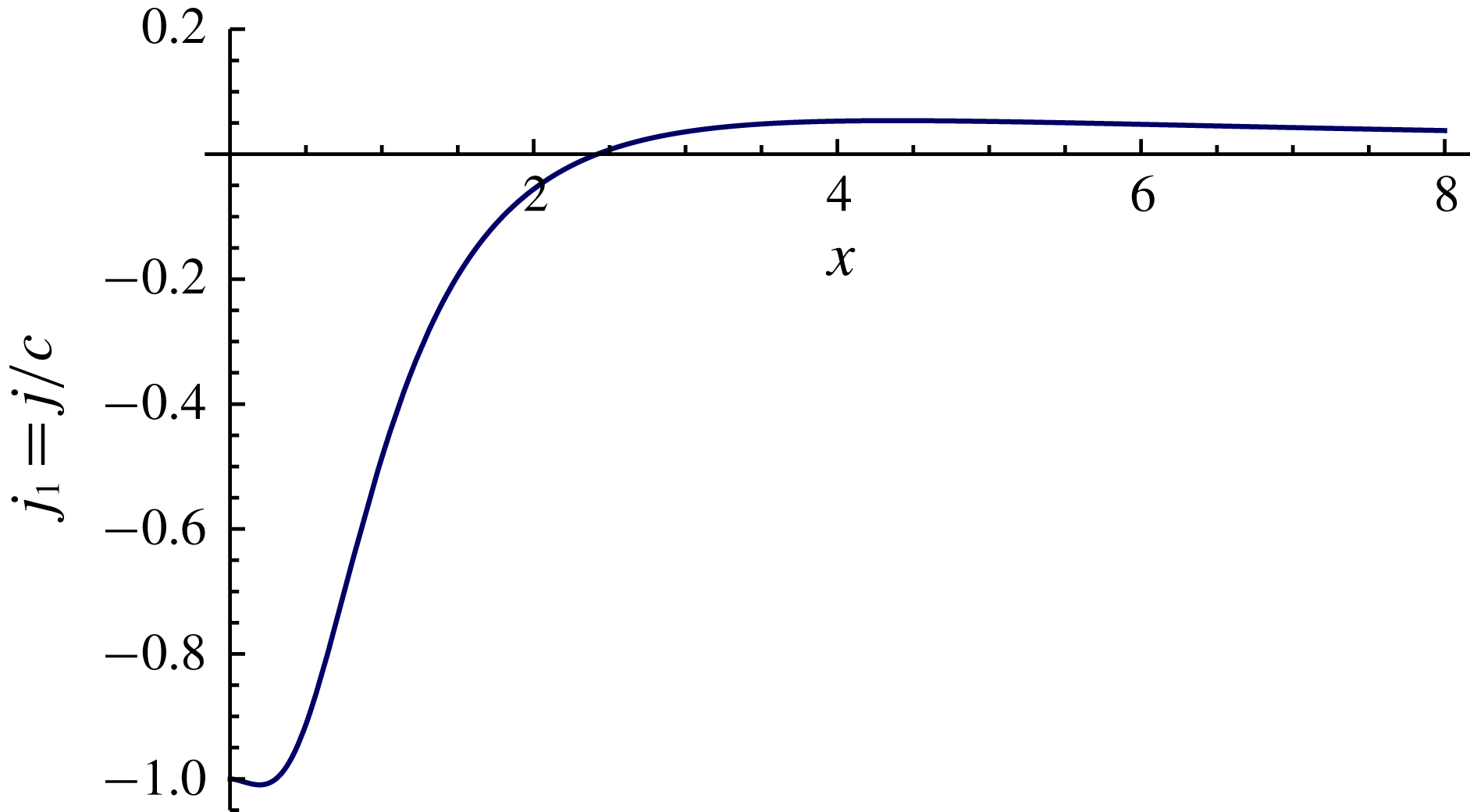
Note that
 $j_{1}$
changes sign at a certain distance from the tip (see figure 9). Furthermore, one can show that
 $$\begin{eqnarray}\int _{0}^{+\infty }j_{1}\,\text{d}x=0,\end{eqnarray}$$
as follows from considerations similar to those that led to (4.7). Thus, for a moving contact line in a saturated atmosphere, evaporation over one part of the microregion is exactly compensated by condensation over the other part, with no overall phase transformation. (Janeček et al. (Reference Janeček, Doumenc, Guerrier and Nikolayev2015) arrive at a similar conclusion in their recent study.) Note that this feature is specific to the present case of diffusion-limited vapour exchange with an inert-gas atmosphere and is not predicted in the case of a pure-vapour atmosphere (Rednikov & Colinet Reference Rednikov and Colinet2013).
4.5 Contact line advancing at a finite velocity for negligible global phase change or saturated atmosphere (case V)
In §§ 4.3 and 4.4 (cases III and IV), contact-line motion was considered as a perturbation upon the microregion structure (
 $c\ll 1$
). Here we at last embark on a case when it is a main (microregion-defining) effect,
 $c=O(1)$
. As in case IV of § 4.4, attention is focused on the situation of no global phase change (
 $E=0$
), which can e.g. imply a saturated atmosphere (
 $\unicode[STIX]{x1D70C}_{v,\infty }^{\ast }=\unicode[STIX]{x1D70C}_{v,sat}^{\ast }$
). As in § 4.4, an interpretation in the sense of the limit of weak phase change,
 $E\ll 1$
, which is then neglected, is also possible here. Unlike § 4.4, however, in the present context it will rather mean that the phase-change-induced film slopes are small first of all against the motion-induced ones in the microregion, but not necessarily against Young’s angle. Thus, there is a priori no evaporative singularity, while we shall again test our Kelvin-only model as far as the resolution of the pure moving contact-line singularity is concerned, now for a stronger case of finite contact-line velocities. Nonetheless, we shall here limit ourselves to advancing contact lines (
 $c>0$
). The present study case is designated as case V in table 1.
Among the motivations for the present case V, we should importantly recall the fact that case IV is actually limited to finite Young’s angles (partial wetting). Hence the regime of perfect wetting is inherently inaccessible from within it (cf. § 4.4). It is different when contact-line motion is regarded as a microregion-defining effect as in the present subsection. Perfect wetting (zero Young’s angle) becomes then just one of the points in the parameter space of the problem, like it was earlier for cases I and III (§§ 4.1 and 4.3).
As the focus here is on advancing contact lines with
 $c=O(1)$
, the principle of dominant balance encourages the scaling
 $c\equiv 1$
(apart from
 ${\mathcal{K}}\equiv 1$
implied throughout). From (2.20), we then obtain
 $$\begin{eqnarray}\unicode[STIX]{x1D716}=(3\,Ca)^{1/3}\quad (\text{scaling}~{\mathcal{K}}\equiv 1,\,c\equiv 1).\end{eqnarray}$$
This is yet another form of
 $\unicode[STIX]{x1D716}$
encountered in the present paper, different from those given earlier by (4.2) and (4.9), and now characterising film slopes induced in the microregion due to contact-line motion. For
 $\unicode[STIX]{x1D717}_{Y}=O(1)$
, these slopes are of the same order as Young’s angle
 $\unicode[STIX]{x1D703}_{Y}$
. Note however that, in view of large logarithm values in (4.20), the motion-induced apparent contact angle is nonetheless generally much greater than the microscopic (Young’s) one in the present case V. Note also that the limit of small velocities (case IV, § 4.4) must correspond, in the present scaling
 $c\equiv 1$
, to
 $\unicode[STIX]{x1D717}_{Y}\gg 1$
(see also below).
With
 $c\equiv 1$
and in view of
 $E=0$
,
 $\unicode[STIX]{x1D717}_{Y}$
remains the only input parameter of the problem, varying in principle from
 $\unicode[STIX]{x1D717}_{Y}=0$
(perfect wetting) to infinity.
Note that, with the help of (4.37), all non-dimensionalisation and angle rescalings can be ultimately specified by means of (2.11) and (2.20)–(2.24), thereby yielding the ensemble of microregion scales determined by the Kelvin effect and the contact-line velocity.
The mathematical formulation corresponding to case V is given by (2.12)–(2.19) with
 $c\equiv 1$
,
 ${\mathcal{K}}\equiv 1$
and
 $E=0$
.
As always in this paper, a special attention is paid to the behaviour near the tip of the film, highlighting the absence of singularities and hence a successful role of the Kelvin effect in this regard. The corresponding coordinate expansions are obtained similarly to (4.4), (4.5), (4.26) and (4.27) as
 $$\begin{eqnarray}h\sim \unicode[STIX]{x1D717}_{Y}x-\frac{1}{6}C_{0}x^{2}-\frac{\unicode[STIX]{x1D717}_{Y}}{18\unicode[STIX]{x03C0}}x^{3}\ln x+\frac{5\unicode[STIX]{x1D717}_{Y}-6\unicode[STIX]{x03C0}C_{1}}{108\unicode[STIX]{x03C0}}x^{3}+\cdots \quad \text{as}~x\rightarrow 0,\end{eqnarray}$$
 $$\begin{eqnarray}\displaystyle \tilde{\unicode[STIX]{x1D70C}}_{v} & {\sim} & \displaystyle C_{0}+\frac{\unicode[STIX]{x1D717}_{Y}}{\unicode[STIX]{x03C0}}r[\ln r\cos \unicode[STIX]{x1D711}-(\unicode[STIX]{x1D711}-\unicode[STIX]{x03C0})\sin \unicode[STIX]{x1D711}]+C_{1}r\cos \unicode[STIX]{x1D711}\nonumber\\ \displaystyle & & \displaystyle -\,\frac{C_{0}}{6\unicode[STIX]{x03C0}}r^{2}[\ln r\cos 2\unicode[STIX]{x1D711}-(\unicode[STIX]{x1D711}-\unicode[STIX]{x03C0})\sin 2\unicode[STIX]{x1D711}]+C_{2}r^{2}\cos 2\unicode[STIX]{x1D711}+\cdots \quad \text{as}~r\rightarrow 0.\qquad\end{eqnarray}$$
As earlier with (4.26) and (4.27), we notice from (4.38) and (4.39) that the behaviour is somewhat more singular now than for an immobile contact line with evaporation, cf. (4.4) and (4.5). It is also more singular than in the similar problem for a pure-vapour atmosphere (Rednikov & Colinet Reference Rednikov and Colinet2013). In particular, the first derivatives of the concentration field or of the pressure in the film (proportional to
 $\text{d}^{3}h/\text{d}x^{3}$
) diverge logarithmically towards the tip. Notwithstanding, this is still far from being any serious singularity, the shear stress on the substrate (2.25) behaving as
 $\unicode[STIX]{x1D70E}_{\unicode[STIX]{x1D70F}}\sim -(1/3)\unicode[STIX]{x03C0}^{-1}\unicode[STIX]{x1D717}_{Y}^{2}x\ln x$
as
 $x\rightarrow 0$
, i.e. vanishing at the contact line and hence being clearly integrable.
The Cox–Voinov relations (4.17), (4.18) and (4.20) still hold, of course, albeit with a twist. Namely, for
 $c=1$
, there is no more separation into the microregion and the Cox–Voinov intermediate region. In particular, intermediate-asymptotic results such as (4.30) no longer make sense. Rather, (4.18) becomes an immediate asymptotic behaviour of the dimensionless microregion solution as
 $x\rightarrow +\infty$
, satisfying the boundary condition (2.14), which is consistent with the asymptotic behaviours found by Duffy & Wilson (Reference Duffy and Wilson1997) for their exact solutions. To ensure representational continuity, we shall still use in (4.17), (4.18) and (4.20) the angles
 $\unicode[STIX]{x1D703}_{mic}$
and
 $\unicode[STIX]{x1D717}_{mic}$
, although in this case there is no longer clear-cut asymptotic distinction between the contributions
 $3c\ln \ell _{mic}$
and
 $\unicode[STIX]{x1D717}_{mic}^{3}$
. Furthermore, since in accordance with considering no global phase change (
 $E=0$
) there are no evaporation-induced contributions, we shall use
 $\unicode[STIX]{x1D703}_{mic}=\unicode[STIX]{x1D703}_{Y}$
and
 $\unicode[STIX]{x1D717}_{mic}=\unicode[STIX]{x1D717}_{Y}$
, with
 $\unicode[STIX]{x1D703}_{Y}=\unicode[STIX]{x1D717}_{Y}=0$
for perfect wetting. The values of
 $\ell _{mic}$
will be obtained as a result of the analysis. As for the behaviour at infinity of the vapour concentration, there is a noteworthy vanishing of the right-hand side of the condition (2.18) in view of the absence of global phase change (
 $E=0$
) assumed here. Therefore, the behaviour of
 $\tilde{\unicode[STIX]{x1D70C}}_{v}$
as
 $r\rightarrow \infty$
will rather be
 $O(r^{-1/2})$
, similar to what was found in (4.29a
). More details about the coordinate expansions at infinity can be found in appendix C.
Numerical solution is constructed for the present case V exactly in the same way as for case I in § 4.1. As in the earlier cases, a numerical solution smoothly adhering to the coordinate expansions is obtained, which is illustrated in figure 10. The computation results for a number of characteristics of interest are shown in figures 11–13.
The same as in figure 2, but now for an advancing contact line under the conditions of negligible global phase change, e.g. a saturated atmosphere (case V of table 1). The coordinate expansions are now given by (4.38) for small
 $x$
and by (C 5) for large
 $x$
(for
 $\unicode[STIX]{x1D717}_{Y}=2$
, the latter expansion coincides to within the line thickness with the numerical result up to small values of
 $x$
).
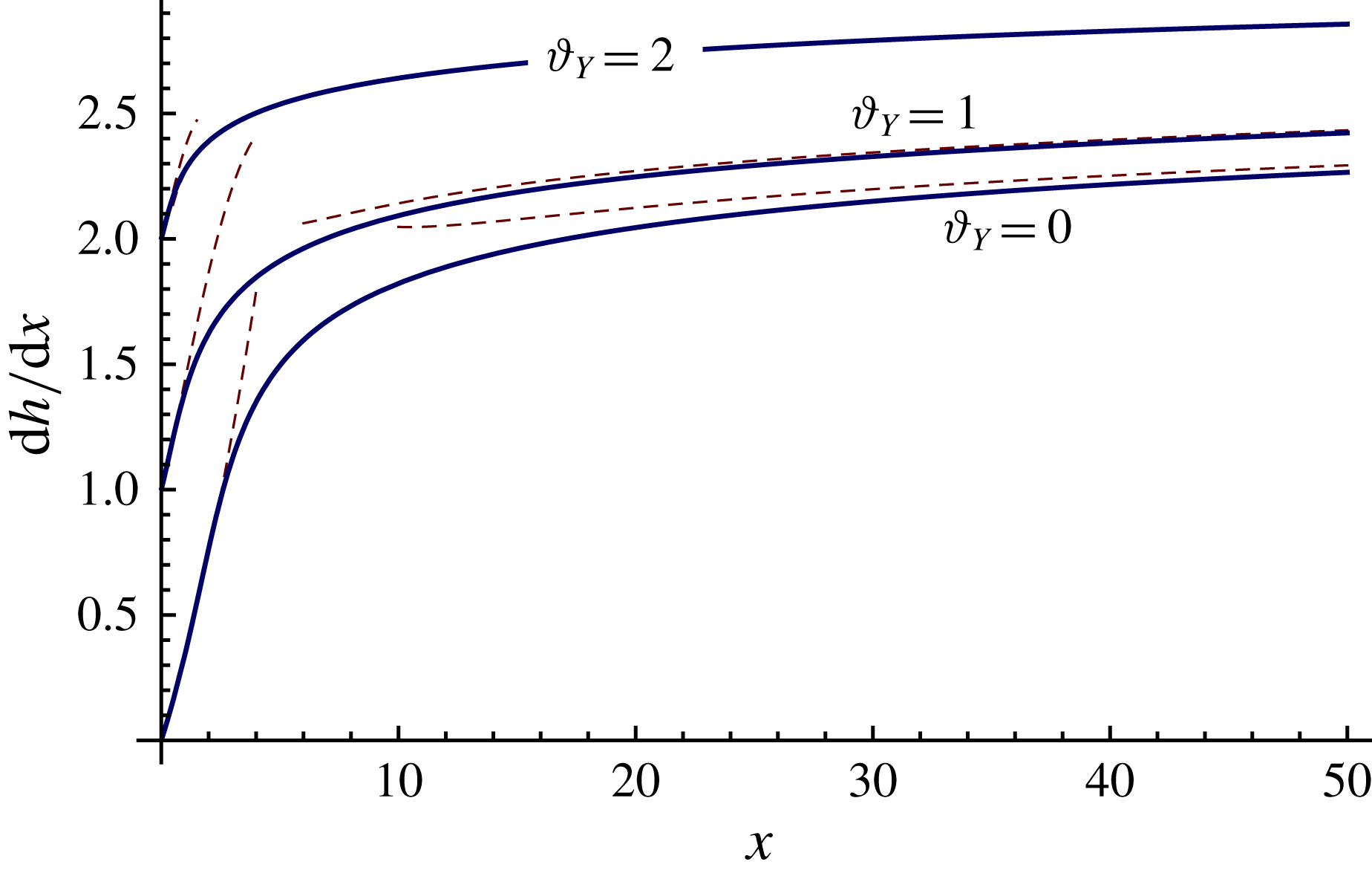
The local phase-change rate profiles are shown in figure 11, for which we notice a change of sign expected in accordance with the property
 $$\begin{eqnarray}\int _{0}^{+\infty }j\,\text{d}x=0.\end{eqnarray}$$
All aspects related to (4.40) are similar to those discussed for (4.7) and (4.36). Figure 11 also confirms that it is by means of condensation that the contact-line advancement is realised not to violate the no-slip condition (
 $j|_{x=0}=-c\,\unicode[STIX]{x1D717}_{Y}<0$
with here
 $c\equiv 1$
at the tip of the film), in line with the corresponding discussion in § 4.4.
Figures 12 and 13 show the computation results for
 $\ell _{mic}$
and
 $C_{0}$
, respectively. (The quantity
 $\unicode[STIX]{x1D717}_{eff}$
(a rescaled ‘effective’ angle) used by Rednikov & Colinet (Reference Rednikov and Colinet2013) is related to
 $\unicode[STIX]{x1D717}_{mic}$
and
 $\ell _{mic}$
by means of
 $\unicode[STIX]{x1D717}_{eff}^{3}=\unicode[STIX]{x1D717}_{mic}^{3}-3c\ln e\ell _{mic}$
, which in the present context with
 $\unicode[STIX]{x1D717}_{mic}=\unicode[STIX]{x1D717}_{Y}$
(no global phase change) and
 $c\equiv 1$
is
 $\unicode[STIX]{x1D717}_{eff}^{3}=\unicode[STIX]{x1D717}_{Y}^{3}-3\ln e\ell _{mic}$
.) The quantity
 $C_{0}$
represents simultaneously the vapour-density deviation from
 $\unicode[STIX]{x1D70C}_{v,sat}^{\ast }$
and the film curvature at the tip as given by (4.38) and (4.39).
Dimensionless local phase-change flux along the microregion of a contact line advancing at a finite velocity in the absence of global phase change (case V of table 1) for a number of values of the rescaled Young’s angle
 $\unicode[STIX]{x1D717}_{Y}=\unicode[STIX]{x1D703}_{Y}/\unicode[STIX]{x1D716}$
. Numerical results.
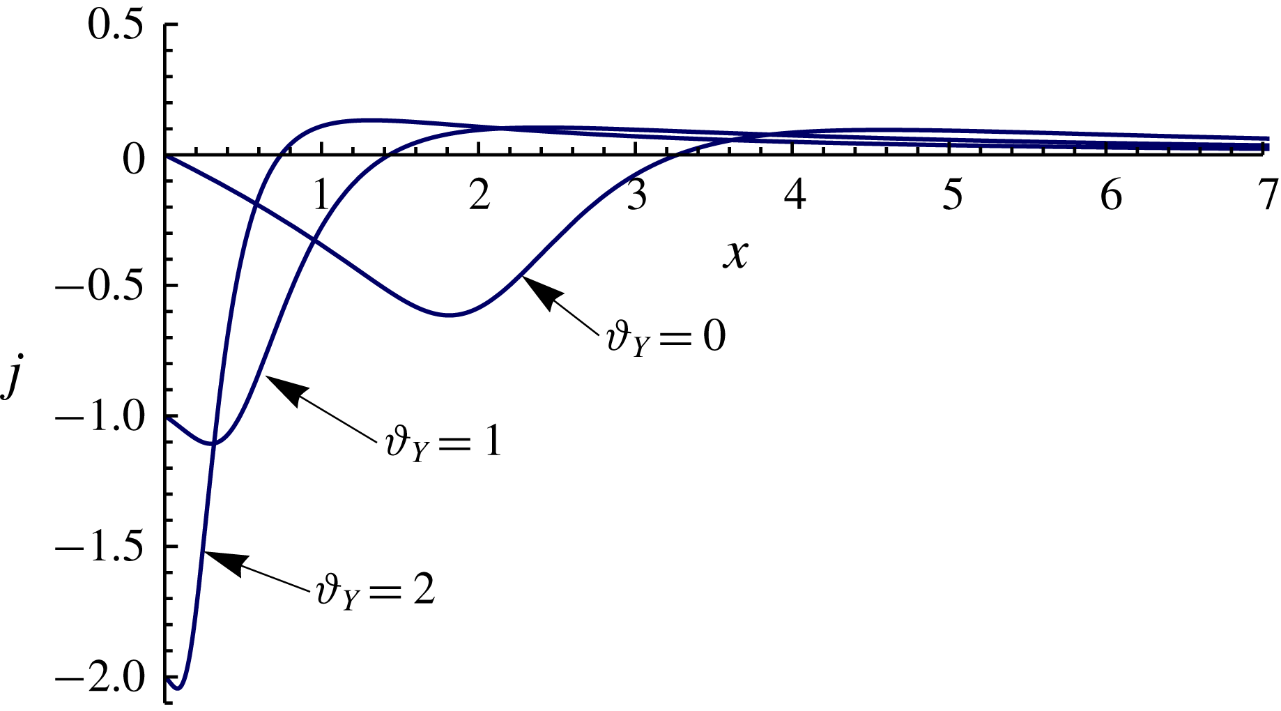
Dimensionless (scale
 $[x]$
) Voinov microlength versus the rescaled Young’s angle
 $\unicode[STIX]{x1D717}_{Y}=\unicode[STIX]{x1D703}_{Y}/\unicode[STIX]{x1D716}$
for a contact line advancing at a finite velocity in the absence of global phase change (case V of table 1), cf. (4.18) where for case V we have
 $c\equiv 1$
and
 $\unicode[STIX]{x1D717}_{mic}=\unicode[STIX]{x1D717}_{Y}$
.

The dependence on the rescaled Young’s angle
 $\unicode[STIX]{x1D717}_{Y}=\unicode[STIX]{x1D703}_{Y}/\unicode[STIX]{x1D716}$
of the value
 $C_{0}=\tilde{\unicode[STIX]{x1D70C}}_{v}|_{r=0}=-3\,\text{d}^{2}h/\text{d}x^{2}|_{x=0}$
(at the tip of the film) as a quantitative indicator of the required strength of the Kelvin effect in the case of a contact line advancing at a finite velocity in the absence of global phase change (case V of table 1).
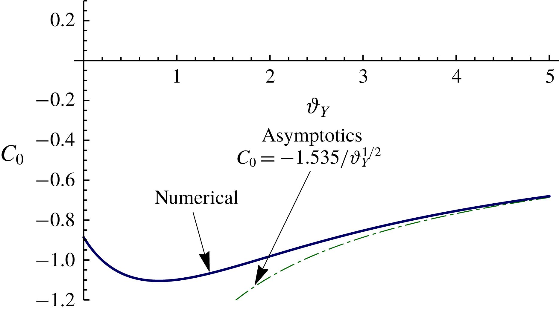
The asymptotic behaviours at
 $\unicode[STIX]{x1D717}_{Y}\gg 1$
also shown in figures 12 and 13 are derived from the results of case IV considered in § 4.4. Indeed,
 $\unicode[STIX]{x1D717}_{Y}\gg 1$
in the present scaling
 $c\equiv 1$
is equivalent to
 $c\ll 1$
(contact-line velocity as a perturbation) in the scaling
 $\unicode[STIX]{x1D717}_{Y}\equiv 1$
considered in § 4.4. Thus, the derivation in question is just a matter of a simple rescaling between the scalings
 $c\equiv 1$
and
 $\unicode[STIX]{x1D717}_{Y}\equiv 1$
, similar to what we already saw in §§ 4.2 and 4.4. Curiously enough, the results of case IV already proved to be pertinent for establishing the asymptotic behaviours in another context as well, namely for case III considered in § 4.3 (see figures 7 and 8).
In relation to a discussion by Eggers & Stone (Reference Eggers and Stone2004), it is interesting to note that the velocity dependence of the (dimensional) microscopic length in the case of perfect wetting is here given by
 $\ell _{mic}^{\ast }=0.47\,\unicode[STIX]{x1D6FF}^{\ast }\,Ca^{-1/2}$
, which follows from
 $\ell _{mic}=0.82$
(cf. figure 12 for
 $\unicode[STIX]{x1D717}_{Y}=0$
), (2.24a
), (4.19) and (4.37). Thus, the present Kelvin-only resolution yields a power law intermediate between
 $\ell _{mic}^{\ast }\propto Ca^{-1/3}$
and
 $\ell _{mic}^{\ast }\propto Ca^{-2/3}$
obtained when the contact-line singularity is taken care of by the Navier slip and by the disjoining pressure, respectively (cf. Hervet & de Gennes (Reference Hervet and de Gennes1984), Hocking (Reference Hocking1992), Eggers & Stone (Reference Eggers and Stone2004), their results being here rewritten in our present notation). In contrast, in the case of a pure-vapour atmosphere, the Kelvin-only consideration (Rednikov & Colinet Reference Rednikov and Colinet2013) leads to the same power law,
 $\ell _{mic}^{\ast }\propto Ca^{-2/3}$
, as the one obtained for the disjoining pressure.
Finally, it is quite noteworthy that even a combination of perfect wetting (
 $\unicode[STIX]{x1D717}_{Y}=0$
) and a saturated atmosphere (
 $E=0$
) does not actually lead to the disappearance of the film tip in the present case of diffusion-limited vapour exchange with an inert-gas medium. This indeed contrasts with what happens in the case of a pure-vapour atmosphere (Rednikov & Colinet Reference Rednikov and Colinet2013). There, it is rather a so-called ‘maximal’ solution that takes over for
 $\unicode[STIX]{x1D717}_{Y}=0$
and
 $E=0$
(a term inspired by Hervet & de Gennes Reference Hervet and de Gennes1984). It can be viewed as if the tip were elongating to
 $x=-\infty$
from the main body of the film. The difference can perhaps most readily be appreciated already when studying possible asymptotic behaviours near the tip. Here, even with
 $\unicode[STIX]{x1D717}_{Y}=0$
and
 $E=0$
, we are able to come up with a non-trivial coordinate expansion for a finite location of the tip (chosen to correspond to
 $x=0$
), cf. (4.38) and (4.39). There (Rednikov & Colinet Reference Rednikov and Colinet2013), this did not appear to be possible.
5 Concluding remarks
We have confirmed that the Kelvin effect alone, without other microphysics effects, can relax contact-line singularities, both phase-change- and motion-related, for both partial-wetting (finite Young’s angle) and perfect-wetting (zero Young’s angle) situations. The present case of diffusion-limited phase change in an inert-gas atmosphere is shown to be similar in this regard, albeit not in fine detail, to the case of conduction-limited phase change in a pure-vapour atmosphere considered elsewhere. The analysis has been accomplished within a minimalist model in the framework of standard hydrodynamics, without any disjoining pressure, precursor film, Navier slip or diffuse interfaces. Even the effect of kinetic resistance to phase change, generally expected to provide an additional regularisation mechanism, was opportunely left out of the model and thus proved inessential for singularity resolution.
Exhaustive parametric studies (with Young’s angle varying from zero to finite values) have been carried out within our Kelvin-only approach for two particular benchmark configurations. One involved an immobile contact line in an undersaturated atmosphere, hence with evaporation occurring at the global scale (case I of table 1). This enabled us to consider the resolution of the evaporative contact-line singularity in its pure form. The main usable output of such a study is the calculated Kelvin-only value of the microregion contact angle (
 $\unicode[STIX]{x1D703}_{mic}$
, and
 $\unicode[STIX]{x1D717}_{mic}$
its rescaled version), an apparent contact angle observed at larger scales. The angle
 $\unicode[STIX]{x1D703}_{mic}$
consists of both Young’s angle and the evaporation-induced contributions, and in the perfect-wetting situation it is evaporation-induced in its entirety.
The other benchmark configuration involved an advancing contact line without any phase change at the global scale, e.g. in a saturated atmosphere (case V). This allowed demonstrating the resolution of moving contact-line singularities in their pure form. It was shown that the contact line advances by local condensation near the tip of the liquid film (and it recedes by local evaporation as shown in cases III and IV discussed below), which is automatically adjusted in this way by the Kelvin effect and which enables the avoiding of singularities despite the no-slip condition at the substrate (where the liquid velocity truly vanishes). The main practical output here is the Kelvin-only value of the microlength
 $\ell _{mic}$
entering the Cox–Voinov relation, hence the scale below which the motion-induced singularity is regularised. Contrary to the many different models alleviating this singularity in the literature, this length scale here only depends on (well-documented) classical macroscopic fluid properties. It is also remarkable that, for this second benchmark configuration, the perfect-wetting case is here not peculiar in the range of finite Young’s angles. In other words, no ‘maximal solution’ structure is formed at zero Young’s angle, quite in contrast with the corresponding finding for a pure-vapour atmosphere (Rednikov & Colinet Reference Rednikov and Colinet2013).
Other studies carried out here include a practically important situation (case III) when the effect of contact-line motion is a perturbation upon the first of the earlier mentioned benchmark configurations. Herewith, the main usable output (beyond just singularity resolution) is the microlength entering the Cox–Voinov relation. The practical importance of this situation is related to its falling under a distinguished asymptotic limit. Indeed, for the motion contribution to be comparable with
 $\unicode[STIX]{x1D703}_{mic}$
within the Cox–Voinov region (a distinguished limit), it must just remain a perturbation in the microregion. Now limited to partial wetting, motion-induced (case IV) and phase-change-induced (case II) perturbations have also been considered upon an equilibrium (trivial) state with no phase change and characterised by a constant film slope everywhere equal to Young’s angle. We note that these perturbative analyses are equally valid for both advancing and receding contact lines (for motion perturbations, case IV), and for both global evaporation and global condensation (for phase-change perturbations, case II). As order-unity effects, contact-line recession and global condensation remained beyond the scope of the present paper, as one can anticipate that these factors may lead for sufficiently small Young’s angles to a breakdown of the contact-line microregion structure assumed here.
The Kelvin-only microregion results developed in the present paper are in fact readily incorporable into global macroscopic models. For instance, they are actually ready to use in the asymptotic framework developed by Saxton et al. (Reference Saxton, Whiteley, Vella and Oliver2016) and Savva et al. (Reference Savva, Rednikov and Colinet2017) for evaporating sessile drops. Thus, at the evaporation (mass loss) stage of their lifetimes, it is the angle
 $\unicode[STIX]{x1D703}_{mic}$
(case I) that will be the apparent contact angle of such drops. At an earlier, fast spreading/retraction stage, it is the microlength
 $\ell _{mic}$
that should be used in the Cox–Voinov relation (case III), apart from the already mentioned
 $\unicode[STIX]{x1D703}_{mic}$
(case I) as the microscopic angle. For a saturated atmosphere and no global phase change, the results of case III degenerate into those of case IV. Still for a saturated atmosphere, the results of case V are to be used at the fast spreading stage either in the case of perfect wetting or when the apparent contact angle of a sessile drop is much greater than its eventual equilibrium (Young’s) one.
The Kelvin effect needs rather small length scales to act and decays fast enough at larger scales, which leads, in spite of the absence of any microphysical effects beyond standard hydrodynamics in the present model, to the existence of a microregion. The question is then whether disregarding such other microphysics effects is physically legitimate. Indeed, even if, in the presence of the Kelvin effect, they are not needed for the resolution of contact-line singularities, they may nonetheless be physically present at those scales and affect the phenomenon. Let us consider, for instance, the disjoining pressure in the form inversely proportional to the cube of the film thickness, in which case a so-called molecular length scale
 $a^{\ast }$
(e.g. de Gennes Reference de Gennes1985; Colinet & Rednikov Reference Colinet and Rednikov2011) is deemed to be the counterpart of the here introduced Kelvin length
 $\unicode[STIX]{x1D6FF}^{\ast }$
(cf. (2.21)). Both these quantities typically belong to a nanometric and subnanometric range and are quite commensurate. Clearly, the present results will tend to be more physically legitimate when
 $\unicode[STIX]{x1D6FF}^{\ast }>a^{\ast }$
. However, it is not just
 $\unicode[STIX]{x1D6FF}^{\ast }$
and
 $a^{\ast }$
that determine the actual microregion size, for an additional scaling with a slope parameter
 $\unicode[STIX]{x1D716}$
is also involved. For instance, the film thickness in the microregion scales as
 $\unicode[STIX]{x1D6FF}^{\ast }/\unicode[STIX]{x1D716}^{1/2}$
in the present study (cf. (2.24)), and as
 $a^{\ast }/\unicode[STIX]{x1D716}$
in the case of the disjoining pressure (e.g. Colinet & Rednikov Reference Colinet and Rednikov2011). Therefore, the present Kelvin-only model is favoured for more volatile liquids (yielding larger evaporation-induced angles, and hence larger
 $\unicode[STIX]{x1D716}$
) and/or for larger Young’s angles, whereas the disjoining-pressure model must clearly overtake in the opposite case. On the other hand, the inverse cubic law of the disjoining pressure is expected to cease to be valid at sufficiently small film thicknesses, where the disjoining pressure in general rather reaches a maximum, and this effect could actually favour the present Kelvin-only model. Further discussion of this issue is beyond the scope of the present paper, whose main goal was rather to highlight the conceptually important self-sufficiency of the Kelvin effect in removing contact-line singularities. In any case, the here obtained Kelvin-only regimes are deemed to be useful at least as noteworthy limiting cases within possibly more general models, in the same way as their counterparts proved to be in the case of a pure-vapour atmosphere (Rednikov & Colinet Reference Rednikov and Colinet2017).
Acknowledgements
The authors gratefully acknowledge financial support of ESA & BELSPO (PRODEX projects), Fonds de la Recherche Scientifique–FNRS (Research Director Position of PC) and BELSPO (IAP 7/38
 $\unicode[STIX]{x1D707}$
-MAST project). This research was also carried out under COST Action MP1106’s umbrella.
Appendix A. Criteria for neglecting thermal effects
We shall assume a sufficiently heat conducting substrate and hence disregard offhand substrate-related temperature non-uniformity. Even so, the latent heat of phase change can lead to temperature variations in the liquid film (cf. Dunn et al. Reference Dunn, Wilson, Duffy, David and Sefiane2009), which can affect the studied phenomena. Below we establish the criteria for such thermal effects to be negligible as assumed throughout the present paper.
A first effect comes through the saturation quantities
 $p_{sat}^{\ast }$
and
 $\unicode[STIX]{x1D70C}_{v,sat}^{\ast }=p_{sat}^{\ast }M^{\ast }/R_{g}^{\ast }T^{\ast }$
, which were here assumed constant and evaluated at the ‘ambient’ temperature, but which are rather sensitive to temperature variations in reality. Let
 $[\tilde{T}]$
be the order of magnitude of temperature variations in the microregion. We estimate
 $\unicode[STIX]{x1D706}_{l}^{\ast }[\tilde{T}]/[h]\sim {\mathcal{L}}^{\ast }[j]$
, implying that the heat of phase change is mainly evacuated by conduction across the liquid film. Here
 $\unicode[STIX]{x1D706}_{l}^{\ast }$
is the liquid thermal conductivity, while
 ${\mathcal{L}}^{\ast }$
(
 $\text{J}~\text{kg}^{-1}$
) is the latent heat. The other notations are the same as in § 2. On the other hand, a diffusion-limited phase change implies
 $[j]\sim D_{g}^{\ast }[\tilde{\unicode[STIX]{x1D70C}}_{v}]/[x]$
. Thus,
 $[\tilde{T}]\sim {\mathcal{L}}^{\ast }D_{g}^{\ast }[\tilde{\unicode[STIX]{x1D70C}}_{v}]\unicode[STIX]{x1D716}/\unicode[STIX]{x1D706}_{l}^{\ast }$
. This brings about a variation of
 $\unicode[STIX]{x1D70C}_{v,sat}^{\ast }$
of the order of
 $[\tilde{T}]\,\text{d}\unicode[STIX]{x1D70C}_{v,sat}^{\ast }/\text{d}T^{\ast }$
. For the thermal effect to be negligible, this variation must be small against
 $[\tilde{\unicode[STIX]{x1D70C}}_{v}]$
, hence a criterion
 $$\begin{eqnarray}\unicode[STIX]{x1D6FC}\unicode[STIX]{x1D716}\ll 1,\quad \text{with}~\unicode[STIX]{x1D6FC}=\frac{{\mathcal{L}}^{\ast 2}M^{\ast }D_{g}^{\ast }\unicode[STIX]{x1D70C}_{v,sat}^{\ast }}{\unicode[STIX]{x1D706}_{l}^{\ast }R_{g}^{\ast }T^{\ast 2}},\end{eqnarray}$$
where we used
 $\text{d}\unicode[STIX]{x1D70C}_{v,sat}^{\ast }/\text{d}T^{\ast }={\mathcal{L}}^{\ast }M^{\ast }\unicode[STIX]{x1D70C}_{v,sat}^{\ast }/R_{g}^{\ast }T^{\ast 2}$
(cf. the Clausius–Clapeyron relation). Not surprisingly, the criterion
 $(\unicode[STIX]{x1D6FC}\unicode[STIX]{x1D716})$
coincides with the Biot number deduced for an evaporating liquid film provided that
 $\unicode[STIX]{x1D716}$
takes the place of the dimensionless wavenumber and the gas thermal conductivity is ultimately neglected (see e.g. Machrafi et al.
Reference Machrafi, Rednikov, Colinet and Dauby2015, and references therein). For the typical parameter values provided below (2.24), as well as
 ${\mathcal{L}}^{\ast }\sim 10^{6}~\text{J}~\text{kg}^{-1}$
and
 $\unicode[STIX]{x1D706}_{l}^{\ast }\sim 0.1~\text{W}~\text{m}^{-1}~\text{K}^{-1}$
, we obtain
 $\unicode[STIX]{x1D6FC}\sim 0.13$
. Thus, the criterion (A 1) is fairly well satisfied, all the more so that
 $\unicode[STIX]{x1D716}$
is a small parameter. In general, its satisfaction tends to deteriorate for more volatile liquids (cf. table 2).
A second thermal effect comes by means of the Marangoni stresses appearing due to the temperature dependence of surface tension,
 $\unicode[STIX]{x1D6FE}^{\ast }=\unicode[STIX]{x1D6FE}_{0}^{\ast }-\unicode[STIX]{x1D6FE}_{T}^{\ast }(T^{\ast }-T_{0}^{\ast })$
, where
 $\unicode[STIX]{x1D6FE}_{0}^{\ast }$
and
 $T_{0}^{\ast }$
are some reference values and typically
 $\unicode[STIX]{x1D6FE}_{T}^{\ast }>0$
(cf. Tsoumpas et al.
Reference Tsoumpas, Dehaeck, Rednikov and Colinet2015). To be negligible in the microregion, the Marangoni stresses must be much smaller than the typical shear stress in the film:
 $\unicode[STIX]{x1D6FE}_{T}^{\ast }[\tilde{T}]/[x]\ll [\unicode[STIX]{x1D70E}_{\unicode[STIX]{x1D70F}}]$
, where
 $[\tilde{T}]={\mathcal{L}}^{\ast }[j][h]/\unicode[STIX]{x1D706}_{l}^{\ast }$
as above, whereas
 $[\unicode[STIX]{x1D70E}_{\unicode[STIX]{x1D70F}}]$
is defined in (2.25b
). Using here
 $[j]$
from (2.22d
) and
 $[h]$
and
 $[x]$
from (2.24), we arrive at
 $$\begin{eqnarray}m\unicode[STIX]{x1D716}^{3/2}\ll 1,\quad \text{with}~m=\frac{\unicode[STIX]{x1D6FE}_{T}^{\ast }{\mathcal{L}}^{\ast }\unicode[STIX]{x1D6FF}^{\ast }}{\unicode[STIX]{x1D706}_{l}^{\ast }\unicode[STIX]{x1D708}_{l}^{\ast }}.\end{eqnarray}$$
For the typical values listed below (2.24) as well as earlier in the present appendix, we obtain
 $m\sim 0.2$
. Thus, also taking into account that
 $\unicode[STIX]{x1D716}$
is a small parameter, the condition (A 2) is seen to hold fairly well. However, just as earlier with (A 1), its quality tends to deteriorate in the case of more volatile liquids (cf. table 2), due to an increase of both
 $\unicode[STIX]{x1D6FF}^{\ast }$
and the evaporation-induced angle scale (4.2) if it is the latter than determines
 $\unicode[STIX]{x1D716}$
in a given situation.
At last, note that it is the latent heat of phase change that was considered as the only source of temperature non-uniformity. One can show that, in spite of the small scales and intense flows in the microregion, viscous dissipation does not contribute as much. Indeed, the latter contribution, per unit area of the film, is of the order of
 $\unicode[STIX]{x1D707}_{l}^{\ast }(\unicode[STIX]{x2202}u/\unicode[STIX]{x2202}z^{\ast })^{2}h^{\ast }\sim \unicode[STIX]{x1D707}_{l}^{\ast -1}\unicode[STIX]{x1D6FE}^{\ast 2}h^{\ast 3}(\unicode[STIX]{x2202}^{3}h^{\ast }/\unicode[STIX]{x2202}x^{\ast 3})^{2}\sim \unicode[STIX]{x1D707}_{l}^{\ast -1}\unicode[STIX]{x1D6FE}^{\ast 2}\unicode[STIX]{x1D716}^{13/2}/\unicode[STIX]{x1D6FF}^{\ast }$
, cf. (2.1c,d
) and (2.24). To justify our approach, this is to be much smaller than
 ${\mathcal{L}}^{\ast }[j]\sim {\mathcal{L}}^{\ast }\unicode[STIX]{x1D6FE}^{\ast }\unicode[STIX]{x1D716}^{4}/\unicode[STIX]{x1D708}_{l}^{\ast }$
, hence a criterion
 $$\begin{eqnarray}{\mathcal{D}}\unicode[STIX]{x1D716}^{5/2}\ll 1,\quad \text{with}~{\mathcal{D}}=\frac{\unicode[STIX]{x1D6FE}^{\ast }}{{\mathcal{L}}^{\ast }\unicode[STIX]{x1D70C}_{l}^{\ast }\unicode[STIX]{x1D6FF}^{\ast }}.\end{eqnarray}$$
With the set of parameter values already used in this appendix, we estimate
 ${\mathcal{D}}\sim 0.1$
, which demonstrates the point.
Appendix B. Estimations for a number of liquids
For various volatile liquids such as HFEs (hydrofluoroether), alkanes and water at roughly the indicated temperatures, table 2 provides the material properties as well as estimations of a number of parameters occurring in the present study. (Here the material properties were principally borrowed from Dehaeck et al. (Reference Dehaeck, Rednikov and Colinet2014) for HFE-7000, Machrafi et al. (Reference Machrafi, Sadoun, Rednikov, Dehaeck, Dauby and Colinet2013) and Tsoumpas et al. (Reference Tsoumpas, Dehaeck, Rednikov and Colinet2015) for HFE-7100, Tsoumpas et al. (Reference Tsoumpas, Dehaeck, Rednikov and Colinet2015) for HFE-7500, www.engineeringtoolbox.com and Lugg (Reference Lugg1968) for pentane, Morris (Reference Morris2014) for octane.)
The Kelvin scale
 $\unicode[STIX]{x1D6FF}^{\ast }$
is clearly seen to increase with the volatility and the molecular weight. For least volatile liquids, it is smaller than the disjoining-pressure-related molecular scale (cf. Morris Reference Morris2014; Jambon-Puillet et al.
Reference Jambon-Puillet, Carrier, Shahidzadeh, Brutin, Eggers and Bonn2018). As a result, the evaporation-induced contact angles
 $\unicode[STIX]{x1D703}_{evap}$
get overestimated within the Kelvin-only approach. For instance, for HFE-7500 they prove to exceed the measured values by
 ${\sim}50\,\%$
, while for HFE-7100 this reduces to
 ${\sim}25\,\%$
(Tsoumpas et al.
Reference Tsoumpas, Dehaeck, Rednikov and Colinet2015). Curiously, for an even more volatile liquid (pentane), the Kelvin-only value of
 $\unicode[STIX]{x1D703}_{evap}$
turns out to agree rather well with the measurements by Jambon-Puillet et al. (Reference Jambon-Puillet, Carrier, Shahidzadeh, Brutin, Eggers and Bonn2018).
Appendix C. Coordinate expansions at infinity
Developing the coordinate expansions behind (2.18) and (4.3) for case I (§ 4.1), one obtains
 $$\begin{eqnarray}\displaystyle h & {\sim} & \displaystyle \unicode[STIX]{x1D717}_{mic}x-\frac{16}{3\unicode[STIX]{x1D717}_{mic}^{3}}x^{1/2}+\bar{s}\ln x+s-\frac{16\bar{s}\ln x}{5\unicode[STIX]{x1D717}_{mic}^{4}x^{1/2}}\nonumber\\ \displaystyle & & \displaystyle +\,\frac{8(15\unicode[STIX]{x1D717}_{mic}^{8}B_{1}-756\unicode[STIX]{x1D717}_{mic}^{7}\bar{s}-90\unicode[STIX]{x1D717}_{mic}^{7}s-2560)}{225\unicode[STIX]{x1D717}_{mic}^{11}x^{1/2}}+\cdots \quad \text{as}~x\rightarrow +\infty ,\end{eqnarray}$$
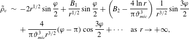 $$\begin{eqnarray}\displaystyle \tilde{\unicode[STIX]{x1D70C}}_{v} & {\sim} & \displaystyle -2r^{1/2}\sin \frac{\unicode[STIX]{x1D711}}{2}+\frac{B_{1}}{r^{1/2}}\sin \frac{\unicode[STIX]{x1D711}}{2}+\left(B_{2}-\frac{4\ln r}{\unicode[STIX]{x03C0}\unicode[STIX]{x1D717}_{mic}^{3}}\right)\frac{1}{r^{3/2}}\sin \frac{3\unicode[STIX]{x1D711}}{2}\nonumber\\ \displaystyle & & \displaystyle +\,\frac{4}{\unicode[STIX]{x03C0}\unicode[STIX]{x1D717}_{mic}^{3}r^{3/2}}(\unicode[STIX]{x1D711}-\unicode[STIX]{x03C0})\cos \frac{3\unicode[STIX]{x1D711}}{2}+\cdots \quad \text{as}~r\rightarrow +\infty ,\end{eqnarray}$$
where
 $\unicode[STIX]{x1D717}_{mic}$
,
 $\bar{s}$
,
 $s$
as well as
 $B_{1}$
,
 $B_{2}$
, etc. are free coefficients to be determined.
The coordinate expansions (4.28) and (4.29) for case III (§ 4.3) are continued as follows:
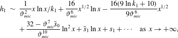 $$\begin{eqnarray}\displaystyle h_{1} & {\sim} & \displaystyle \frac{1}{\unicode[STIX]{x1D717}_{mic}^{2}}x\ln x/k_{1}+\frac{16}{\unicode[STIX]{x1D717}_{mic}^{6}}x^{1/2}\ln x-\frac{16(9\ln k_{1}+10)}{9\unicode[STIX]{x1D717}_{mic}^{6}}x^{1/2}\nonumber\\ \displaystyle & & \displaystyle +\,\frac{32-\unicode[STIX]{x1D717}_{mic}^{7}\bar{s}_{0}}{\unicode[STIX]{x1D717}_{mic}^{10}}\ln ^{2}x+\bar{s}_{1}\ln x+s_{1}+\cdots \quad \text{as}~x\rightarrow +\infty ,\end{eqnarray}$$
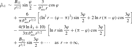 $$\begin{eqnarray}\displaystyle \tilde{\unicode[STIX]{x1D70C}}_{v1} & {\sim} & \displaystyle \frac{B_{11}}{r^{1/2}}\sin \frac{\unicode[STIX]{x1D711}}{2}-\frac{3}{\unicode[STIX]{x1D717}_{mic}^{2}r}\cos \unicode[STIX]{x1D711}\nonumber\\ \displaystyle & & \displaystyle +\,\frac{6}{\unicode[STIX]{x03C0}\unicode[STIX]{x1D717}_{mic}^{6}r^{3/2}}\left[(\ln ^{2}r-(\unicode[STIX]{x1D711}-\unicode[STIX]{x03C0})^{2})\sin \frac{3\unicode[STIX]{x1D711}}{2}+2\ln r\,(\unicode[STIX]{x03C0}-\unicode[STIX]{x1D711})\cos \frac{3\unicode[STIX]{x1D711}}{2}\right]\nonumber\\ \displaystyle & & \displaystyle -\,\frac{4(9\ln k_{1}+10)}{3\unicode[STIX]{x03C0}\unicode[STIX]{x1D717}_{mic}^{6}r^{3/2}}\left[\ln r\sin \frac{3\unicode[STIX]{x1D711}}{2}+(\unicode[STIX]{x03C0}-\unicode[STIX]{x1D711})\cos \frac{3\unicode[STIX]{x1D711}}{2}\right]\nonumber\\ \displaystyle & & \displaystyle +\,\frac{B_{21}}{r^{3/2}}\sin \frac{3\unicode[STIX]{x1D711}}{2}+\cdots \quad \text{as}~r\rightarrow +\infty ,\end{eqnarray}$$
where
 $k_{1}$
,
 $\bar{s}_{1}$
,
 $s_{1}$
,
 $B_{11}$
and
 $B_{21}$
are free coefficients to be determined, whereas
 $\unicode[STIX]{x1D717}_{mic}$
and
 $\bar{s}_{0}$
(the same as
 $\bar{s}$
in (C 1) in accordance with the 0-subscript convention of § 4.3) are here considered known from case I (§ 4.1).
A more detailed version of the coordinate expansions at infinity for case V (§ 4.5) is
 $$\begin{eqnarray}\displaystyle h & {\sim} & \displaystyle x(3\ln x/e\ell _{mic}+\unicode[STIX]{x1D717}_{Y}^{3})^{1/3}\left[1-\frac{10}{3}\frac{1}{(3\ln x/e\ell _{mic}+\unicode[STIX]{x1D717}_{Y}^{3})^{2}}+O\left(\frac{1}{(3\ln x/e\ell _{mic}+\unicode[STIX]{x1D717}_{Y}^{3})^{4}}\right)\right]\nonumber\\ \displaystyle & & \displaystyle +\,\cdots \quad \text{as}~x\rightarrow +\infty ,\end{eqnarray}$$
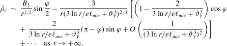 $$\begin{eqnarray}\displaystyle \tilde{\unicode[STIX]{x1D70C}}_{v} & {\sim} & \displaystyle \frac{B_{1}}{r^{1/2}}\sin \frac{\unicode[STIX]{x1D711}}{2}-\frac{3}{r(3\ln r/e\ell _{mic}+\unicode[STIX]{x1D717}_{Y}^{3})^{2/3}}\left[\left(1-\frac{2}{3\ln r/e\ell _{mic}+\unicode[STIX]{x1D717}_{Y}^{3}}\right)\cos \unicode[STIX]{x1D711}\right.\nonumber\\ \displaystyle & & \displaystyle +\left.\frac{2}{3\ln r/e\ell _{mic}+\unicode[STIX]{x1D717}_{Y}^{3}}(\unicode[STIX]{x03C0}-\unicode[STIX]{x1D711})\sin \unicode[STIX]{x1D711}+O\left(\frac{1}{(3\ln r/e\ell _{mic}+\unicode[STIX]{x1D717}_{Y}^{3})^{2}}\right)\right]\nonumber\\ \displaystyle & & \displaystyle +\,\cdots \quad \text{as}~r\rightarrow +\infty .\end{eqnarray}$$