1 Introduction
Turbulence prevails in the Universe, and its multi-scale properties affect the global dynamics of geophysical, astrophysical and industrial flows. Typically, in a turbulent flow, energy is supplied at some scale and is redistributed among scales due to nonlinear interactions between eddies of similar size. This mechanism of energy transfer from large to small scales or vice versa is known as a forward or inverse cascade, respectively. A prominent example of a forward cascade is met in three-dimensional (3-D) hydrodynamic turbulence (Frisch Reference Frisch1995). The turbulent cascade in this case transports the energy from the large (possibly coherent) structures to small ‘incoherent’ scales. An example of an inverse cascade is given by 2-D hydrodynamic turbulence that cascades energy to the large scales (Boffetta & Ecke Reference Boffetta and Ecke2012). There are some examples, however, that have a mixed behaviour, such as rapidly rotating fluids, conducting fluids in the presence of strong magnetic fields, flows in a constrained geometry and others. In these examples the injected energy cascades both forward and inversely in fractions that depend on the value of a control parameter (rotation rate/magnetic field/aspect ratio/etc.). These system thus exhibit a bidirectional cascade: coexistence of a forward and an inverse cascade of energy whose relative amplitudes depend on parameters of the system.
Bidirectional cascades have been observed in different physical situations both in numerical simulations (Smith, Chasnov & Waleffe Reference Smith, Chasnov and Waleffe1996; Smith & Waleffe Reference Smith and Waleffe1999; Celani, Musacchio & Vincenzi Reference Celani, Musacchio and Vincenzi2010; Alexakis Reference Alexakis2011; Sen et al. Reference Sen, Mininni, Rosenberg and Pouquet2012; Marino et al. Reference Marino, Mininni, Rosenberg and Pouquet2013; Pouquet & Marino Reference Pouquet and Marino2013; Deusebio et al. Reference Deusebio, Boffetta, Lindborg and Musacchio2014; Seshasayanan, Benavides & Alexakis Reference Seshasayanan, Benavides and Alexakis2014; Marino, Pouquet & Rosenberg Reference Marino, Pouquet and Rosenberg2015; Rosenberg et al. Reference Rosenberg, Pouquet, Marino and Mininni2015; Sozza et al. Reference Sozza, Boffetta, Muratore-Ginanneschi and Musacchio2015; Seshasayanan & Alexakis Reference Seshasayanan and Alexakis2016) and in laboratory experiments (Shats, Byrne & Xia Reference Shats, Byrne and Xia2010; Byrne, Xia & Shats Reference Byrne, Xia and Shats2011; Xia et al. Reference Xia, Byrne, Falkovich and Shats2011; Yarom, Vardi & Sharon Reference Yarom, Vardi and Sharon2013; Campagne et al. Reference Campagne, Gallet, Moisy and Cortet2014). They are relevant in atmospheric physics where, at large scales, the atmosphere cascades energy inversely due to the combined effect of rotation, stratification and vertical confinement similar to a two-dimensional flow, while at the same time at small scales it cascades energy to even smaller scales, like a three-dimensional (3-D) flow. These coexisting forward and inverse cascades have been quantified with in situ aircraft measurements in the hurricane boundary layer (Byrne & Zhang Reference Byrne and Zhang2013). Similar behaviour has been claimed in astrophysical flows (such as the atmosphere of Venus (Izakov Reference Izakov2013) and accretion discs (Lesur & Longaretti Reference Lesur and Longaretti2011)) and industrial applications (such as tokamak plasma flows (Diamond et al. Reference Diamond, Itoh, Itoh and Hahm2005)) either due to the thinness of the layer, fast rotation or the presence of strong magnetic fields.
This work focuses on one of the simplest setups that exhibits such a transition: turbulence in a thin layer. By thin layer we refer to a 3-D domain that extends to large distances
 $L$
in two (horizontal) directions and short distance
 $H$
in the third (vertical) direction. In such a system eddies with scales
 $\ell$
much larger than the layer thickness
 $H\ll \ell$
are constrained to two-dimensional dynamics while small eddies in the opposite limit
 $\ell \ll H$
do not to feel this constraint and behave like a 3-D flow. This system was first examined by Celani et al. (Reference Celani, Musacchio and Vincenzi2010) where it was shown that for large
 $Re$
the direction of the energy cascade depends on the ratio
 $Q=\ell _{f}/H$
of the horizontal length scale of the forcing
 $\ell _{f}$
to the layer height
 $H$
. Alternatively,
 $Q$
can be considered as the ratio of the smallest non-zero vertical wavenumber to the forcing wavenumber. For
 $Q\gg 1$
 $(\ell _{f}\gg H)$
the energy is injected in eddies that fall in the first regime (two-dimensional) and therefore the cascade is inverse, while for
 $Q\ll 1$
 $(\ell _{f}\ll H)$
the energy is injected in eddies that fall in the second regime (three-dimensional) and therefore the cascade is forward. At intermediate values however the system displays a bidirectional cascade (Celani et al.
Reference Celani, Musacchio and Vincenzi2010).
In this work we will focus on the exact way that the system transitions from a unidirectional to a bidirectional cascade. There are three possible scenarios for such a transition. (i) The transition happens in a smooth way. In this case the amplitude of the inverse or forward cascade decreases smoothly as
 $Q$
is varied (possibly as a power law) and therefore the inverse cascade becomes zero only at the limit
 $Q\rightarrow 0$
while the forward cascade becomes zero only at the opposite limit
 $Q\rightarrow \infty$
. (ii) The transition happens at a critical value
 $Q=Q_{c}$
in a discontinuous way, much like a subcritical instability or a first-order phase transition, so that the system changes abruptly from an inverse cascade to a forward cascade. (iii) The amplitude of the inverse/forward cascade decreases/increases continuously as
 $Q$
is increased and at a critical point
 $Q_{c}$
the inverse/forward cascade becomes exactly zero with discontinuous or diverging derivatives much like a supercritical instability or a second-order phase transition. In the work of Celani et al. (Reference Celani, Musacchio and Vincenzi2010) it was conjectured that the third scenario, (iii), is observed for the transition from a forward unidirectional cascade to a bidirectional cascade although their data did not allow a precise conclusion to be drawn.
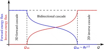
An illustration of the expected critical transitions, corresponding to scenario (iii) described in the text.
 $Q=\ell _{f}/H$
is the ratio of the horizontal length scale of the forcing
 $\ell _{f}$
to the layer height
 $H$
.

For the case of a critical transition there a few remarks that we need to make. These systems transition from one turbulent state that cascades energy inversely, say, to the large scales to a different turbulent state that cascades energy forward to the small scales. Turbulence is thus always present! This makes the discussed transition far different from the traditional scenarios of transition from a laminar to a turbulent state. Turbulent fluctuations are always present and constitute an integral part of the mechanism for the transition, much like how thermal fluctuations play a determinant role in equilibrium phase transitions close to criticality.
For turbulence in thin layers we expect two critical values of
 $Q$
to exist. The first,
 $Q_{3D}$
, marks the transition from purely forward to a bidirectional cascade, whereas the second one,
 $Q_{2D}$
, marks the transition from a bidirectional cascade to a purely inverse cascade. In more detail, for flows of large Reynolds number and for layers sufficiently thick
 $Q\ll 1$
we expect that all energy cascades towards the small scales and no energy to the large scales. As
 $Q$
is increased, and thus the layer made thinner, a critical value
 $Q_{3D}$
will be met for which the appearance of an inverse cascade will begin in coexistence with the forward cascade. This marks the beginning of the bidirectional cascade. As
 $Q$
is increased further the forward cascade decreases while the inverse cascade increases. We then expect a second critical height
 $Q_{2D}$
where the forward cascade becomes zero and all the energy cascades to the large scales. Further increase of
 $Q$
will not alter this behaviour. The bidirectional cascades then exist in the range
 $Q_{3D}<Q<Q_{2D}$
. An illustration of this expectation is shown in figure 1.
The purpose of the present work is to focus on the two critical points: unravel their statistical behaviour as well as study the mechanisms involved close to criticality. Performing such a study with direct numerical simulations of the 3-D Navier–Stokes equation is computationally costly due to the high degree of resolution required in order to have both large enough Reynolds number so that the flow is turbulent and large enough scale separation
 $L\gg \ell _{f}$
so that an inverse cascade develops. To overcome this difficulty we will instead focus on a model of the Navier–Stokes equation. In our model we will keep a minimal description for the vertical direction by performing a drastic Galerkin truncation in the vertical direction keeping only two modes
 $\boldsymbol{u}_{2D}(t,x,y)$
and
 $\boldsymbol{u}_{q}(t,x,y,z)$
. The first mode corresponds to purely 2-D motions and depends only on the horizontal directions
 $(x,y)$
, while the second mode corresponds to a flow whose vertical structure is proportional to
 $\sin (qz)$
or
 $\cos (qz)$
and has arbitrary dependence in the horizontal directions.
The rest of this paper is structured as follows. Section 2 describes our model of thin layer turbulence, as well as our methodology, explaining our measures of the inverse and forward energy cascades (acting as order parameters) as well as the simulation details themselves. Section 3 presents the results and analysis of our investigation of the transition from a purely forward energy cascade to a bidirectional energy cascade. Section 4 focuses on the other transition between a bidirectional cascade and a pure inverse cascade. Finally, in § 5 we summarize our findings and give concluding remarks regarding the results.
2 Model description and methodology
We consider an incompressible flow in a thin layer of thickness
 $H=\unicode[STIX]{x03C0}/q$
in the vertical direction (
 $z$
) and of size
 $2\unicode[STIX]{x03C0}L$
in the remaining two directions
 $(x,y)$
with free slip boundary conditions
 $\unicode[STIX]{x2202}_{z}u_{x}=\unicode[STIX]{x2202}_{z}u_{y}=u_{z}=0$
at
 $z=\pm H/2$
. The flow velocity
 $\boldsymbol{u}$
is governed by the Navier–Stokes equations:
 $$\begin{eqnarray}\displaystyle & \displaystyle \unicode[STIX]{x2202}_{t}\boldsymbol{u}+\boldsymbol{u}\boldsymbol{\cdot }\unicode[STIX]{x1D735}\boldsymbol{u}=-\unicode[STIX]{x1D735}P+\unicode[STIX]{x1D708}\unicode[STIX]{x0394}\boldsymbol{u}+\boldsymbol{F}, & \displaystyle\end{eqnarray}$$
 $$\begin{eqnarray}\displaystyle & \displaystyle \unicode[STIX]{x1D735}\boldsymbol{\cdot }\boldsymbol{u}=0, & \displaystyle\end{eqnarray}$$
where
 $\unicode[STIX]{x1D708}$
is the kinematic viscosity,
 $P$
is the pressure and
 $\boldsymbol{F}$
is a two-dimensional forcing (varying only along
 $x$
and
 $y$
) that acts at a particular horizontal length scale
 $\ell _{f}$
.
As discussed in § 1, in this work we do not solve for the full system requiring 3-D numerical simulations, but we rather focus on a model that is obtained by a severe Galerkin truncation in the vertical direction such that only two modes are kept. The first mode
 $\boldsymbol{u}_{2D}$
has two components that are obtained by vertically averaging
 $u_{x}$
and
 $u_{y}$
. This corresponds to a purely 2-D flow which thus satisfies the incompressibility condition
 $\unicode[STIX]{x1D735}\boldsymbol{\cdot }\boldsymbol{u}_{2D}=0$
. This allows us to write
 $\boldsymbol{u}_{2D}$
in terms of a streamfunction
 $\unicode[STIX]{x1D713}(t,x,y)$
as indicated in (2.3). The second mode
 $\boldsymbol{u}_{q}$
has all three components and a prescribed vertical dependence as given below:
 $$\begin{eqnarray}\boldsymbol{u}_{2D}(t,x,y)=\left(\begin{array}{@{}c@{}}\unicode[STIX]{x2202}_{y}\unicode[STIX]{x1D713}\\ -\unicode[STIX]{x2202}_{x}\unicode[STIX]{x1D713}\\ 0\end{array}\right),\quad \boldsymbol{u}_{q}(t,x,y,z)=\left(\begin{array}{@{}c@{}}v_{x}(x,y,t)\sin (qz)\\ v_{y}(x,y,t)\sin (qz)\\ v_{z}(x,y,t)\cos (qz)\end{array}\right).\end{eqnarray}$$
The vector field
 $\boldsymbol{u}_{q}$
satisfies free slip boundary conditions at
 $z=\pm H/2$
and the incompressibility condition
 $\unicode[STIX]{x1D735}\boldsymbol{\cdot }\boldsymbol{u}_{q}=0$
that, in terms of
 $\boldsymbol{v}_{q}(t,x,y)=(v_{x},v_{y},v_{z})$
, is written as
 $\unicode[STIX]{x2202}_{x}v_{x}+\unicode[STIX]{x2202}_{y}v_{y}=qv_{z}$
. With this notation the truncated Navier–Stokes equations can be written as
 $$\begin{eqnarray}\displaystyle & \displaystyle \unicode[STIX]{x2202}_{t}\boldsymbol{u}_{2D}+\boldsymbol{u}_{2D}\boldsymbol{\cdot }\unicode[STIX]{x1D735}\boldsymbol{u}_{2D}=-\overline{\boldsymbol{u}_{q}\boldsymbol{\cdot }\unicode[STIX]{x1D735}\boldsymbol{u}_{q}}-\overline{\unicode[STIX]{x1D735}P}+\unicode[STIX]{x1D708}\unicode[STIX]{x0394}\boldsymbol{u}_{2D}-\unicode[STIX]{x1D707}\unicode[STIX]{x1D6E5}^{-2}\boldsymbol{u}_{2D}+\boldsymbol{F}, & \displaystyle\end{eqnarray}$$
 $$\begin{eqnarray}\displaystyle & \displaystyle \unicode[STIX]{x2202}_{t}\boldsymbol{u}_{q}+\boldsymbol{u}_{2D}\boldsymbol{\cdot }\unicode[STIX]{x1D735}\boldsymbol{u}_{q}=-\boldsymbol{u}_{q}\boldsymbol{\cdot }\unicode[STIX]{x1D735}\boldsymbol{u}_{2D}-\unicode[STIX]{x1D735}p_{q}+\unicode[STIX]{x1D708}\unicode[STIX]{x0394}\boldsymbol{u}_{q}, & \displaystyle\end{eqnarray}$$
where the overbar stands for vertical averaging
 $\overline{f}\equiv (1/H)\int f\,\text{d}z$
and
 $p_{q}$
is the partial pressure that guarantees the incompressibility of
 $\boldsymbol{u}_{q}$
. Note that if one plugs in
 $\boldsymbol{u}_{q}$
from (2.3) into (2.5), the vertical dependence drops out and we are left with two coupled partial differential equations that depend only on the horizontal directions
 $(x,y)$
. We note that our model is rigorously valid for very thin layers where
 $1/q$
is of the order of the viscous length scales, in which case it can be derived based on an asymptotic expansion, using the thinness of the layer as a small parameter. Despite the lack of rigor for thicker layers, as we will show later, this model is able to capture the relevant physical processes and display a rich behaviour.
Furthermore, note that in our system we have included the hypo-dissipation term
 $\unicode[STIX]{x1D707}\unicode[STIX]{x1D6E5}^{-2}\boldsymbol{u}_{2D}$
that is responsible for saturating the inverse cascade when present. If such a term is absent in the presence of an inverse cascade the energy of the large-scale modes will grow to very large values forming a condensate (Chertkov et al.
Reference Chertkov, Connaughton, Kolokolov and Lebedev2007; Boffetta & Ecke Reference Boffetta and Ecke2012; Laurie et al.
Reference Laurie, Boffetta, Falkovich, Kolokolov and Lebedev2014) whose amplitude growth is balanced by the small viscous forces. These two cases correspond to two very different situations. In the first, there is a constant flux of energy to the large scales while in the second situation the system reaches an almost thermal equilibrium with a non-constant and very weak (compared to the amplitude of the fluctuations) inverse flux of energy. Although both cases are physically relevant, in this work we only focus on the first situation and in all our runs
 $\unicode[STIX]{x1D707}$
is tuned so that the largest scale is sufficiently suppressed.
In the absence of forcing and dissipation terms this system conserves the total energy of the flow given by
 $$\begin{eqnarray}E={\textstyle \frac{1}{2}}\langle |\boldsymbol{u}_{2D}|^{2}+|\boldsymbol{u}_{q}|^{2}\rangle ={\textstyle \frac{1}{2}}\langle |\unicode[STIX]{x1D735}\unicode[STIX]{x1D713}|^{2}\rangle +{\textstyle \frac{1}{4}}\langle v_{x}^{2}+v_{y}^{2}+v_{z}^{2}\rangle ,\end{eqnarray}$$
where angular brackets
 $\langle \boldsymbol{\cdot }\rangle$
stand for spatial average. For
 $\boldsymbol{u}_{q}=0$
one recovers the two-dimensional Navier–Stokes equation in which case the enstrophy
 $\unicode[STIX]{x1D6FA}=\langle |\unicode[STIX]{x1D735}\times \boldsymbol{u}_{2D}|^{2}\rangle /2=\langle |\unicode[STIX]{x0394}\unicode[STIX]{x1D713}|^{2}\rangle /2$
is also conserved. In the presence of forcing and dissipation the system eventually reaches a steady state where the energy injected by the forcing at the averaged rate
 $I=\langle \boldsymbol{F}\boldsymbol{\cdot }\boldsymbol{u}_{2D}\rangle _{T}$
is balanced by the dissipation rates
 $\unicode[STIX]{x1D716}_{3D}^{+}$
,
 $\unicode[STIX]{x1D716}_{2D}^{+}$
, and
 $\unicode[STIX]{x1D716}_{2D}^{-}$
due to viscous and hypo-viscous forces defined as:
 $$\begin{eqnarray}\unicode[STIX]{x1D716}_{2D}^{+}=\unicode[STIX]{x1D708}\langle |\unicode[STIX]{x1D735}\times \boldsymbol{u}_{2D}|^{2}\rangle _{T},\quad \unicode[STIX]{x1D716}_{3D}^{+}=\unicode[STIX]{x1D708}\langle |\unicode[STIX]{x1D735}\times \boldsymbol{u}_{q}|^{2}\rangle _{T},\quad \unicode[STIX]{x1D716}_{2D}^{-}=\unicode[STIX]{x1D707}\langle |\unicode[STIX]{x1D6E5}^{-1}\boldsymbol{u}_{2D}|^{2}\rangle _{T},\end{eqnarray}$$
where the brackets
 $\langle \boldsymbol{\cdot }\rangle _{T}$
indicate space and time average. The dissipation rate
 $\unicode[STIX]{x1D716}_{2D}^{+}$
measures the rate energy is dissipated at the small scales of the 2-D velocity field
 $\boldsymbol{u}_{2D}$
, while
 $\unicode[STIX]{x1D716}_{3D}^{+}$
measures the rate energy is dissipated by the 3-D field
 $\boldsymbol{u}_{q}$
. Finally
 $\unicode[STIX]{x1D716}_{2D}^{-}$
measures the rate energy is dissipated at the large scales of the 2-D velocity field. At steady state a balance is reached and we obtain:
 $$\begin{eqnarray}I=\unicode[STIX]{x1D716}_{2D}^{+}+\unicode[STIX]{x1D716}_{3D}^{+}+\unicode[STIX]{x1D716}_{2D}^{-}.\end{eqnarray}$$
Thus, with a large enough scale separation
 $L\gg \ell _{f}$
, the ratio
 $\unicode[STIX]{x1D716}_{2D}^{-}/I$
provides us with a measure of what fraction of the energy injected is cascading to the large scales. On the other hand, at high enough Reynolds numbers, the ratios
 $\unicode[STIX]{x1D716}_{2D}^{+}/I$
and
 $\unicode[STIX]{x1D716}_{3D}^{+}/I$
provide us with the fraction of the energy that cascades to the small scales.
We need to stress here the importance of considering the large Reynolds number and large-box limit. Here by large-box limit we refer to the horizontal dimensions of the box
 $L\rightarrow \infty$
and not
 $H$
, which is considered fixed in this limiting procedure. In 2-D turbulence there is always some forward transfer of energy that is required to sustain the forward cascade of enstrophy. Similarly, in 3-D turbulence in the presence of a hypo-dissipation term there is an inverse transfer of energy that is needed to sustain the energy at large scales against any dissipative mechanism that removes energy from these scales. These forward and inverse transfers, however, depend on the amplitude of the dissipation coefficients and the box size. When the dissipation coefficients are decreased and the box size is increased, their amplitude decreases to zero (see discussions in Eyink (Reference Eyink1996), Boffetta & Musacchio (Reference Boffetta and Musacchio2010), Boffetta & Ecke (Reference Boffetta and Ecke2012)). Thus, in order to distinguish a weak inverse cascade from these finite size effects we need to demonstrate that
 $\unicode[STIX]{x1D716}_{2D}^{-}$
remains finite as the box size is increased and the hypo-dissipation is decreased. Similarly for
 $\unicode[STIX]{x1D716}_{2D}^{+}$
and
 $\unicode[STIX]{x1D716}_{3D}^{+}$
, we need to investigate their large Reynolds number behaviour.
Two different forcing functions were used in this study. The first was a deterministic time-independent forcing explicitly given by
 $$\begin{eqnarray}\boldsymbol{F}=F_{0}[\cos (k_{f}y),-\cos (k_{f}x),0],\end{eqnarray}$$
where
 $F_{0}$
is the forcing amplitude and
 $k_{f}=\unicode[STIX]{x03C0}/\ell _{f}$
is the forcing wavenumber. It corresponds to forcing a square array of vortices with alternating sign of vorticity. This forcing, although more physical than our second choice, does not inject energy at a constant rate since the injection rate depends on the particular flow realization.
For a better control of the energy injection rate in our system a second type of forcing was used that was designed to inject energy at a given shell of wavenumbers of modulus
 $k_{f}$
at a constant rate at each instant of time and for every realization. It is written as
 $$\begin{eqnarray}\boldsymbol{F}=I_{0}\mathop{\sum }_{|\boldsymbol{k}|=k_{f}}\frac{\tilde{\boldsymbol{u}}_{2D}(\boldsymbol{k})\text{e}^{\text{i}\boldsymbol{k}\boldsymbol{\cdot }x}}{\displaystyle \mathop{\sum }_{|\boldsymbol{k}^{\prime }|=k_{f}}|\tilde{\boldsymbol{u}}_{2D}(\boldsymbol{k}^{\prime })|^{2}}+\text{i}\mathop{\sum }_{|\boldsymbol{k}|=k_{f}}\unicode[STIX]{x1D6FA}_{\boldsymbol{k}}\tilde{\boldsymbol{u}}_{2D}(\boldsymbol{k})\text{e}^{\text{i}\boldsymbol{k}\boldsymbol{\cdot }x},\end{eqnarray}$$
where
 $\tilde{\boldsymbol{u}}_{2D}(\boldsymbol{k})$
stands for the Fourier transform of the field
 $\boldsymbol{u}_{2D}$
. The sums are over all wavenumbers that satisfy
 $|\boldsymbol{k}|=k_{f}$
, and
 $\unicode[STIX]{x1D6FA}_{\boldsymbol{k}}$
is a random frequency that takes values between 1 and
 $-$
1 (for
 $|\boldsymbol{k}|=k_{f}$
and zero otherwise) and leads to a decorrelation of the phases between the different forced modes. The total energy injection rate for this forcing at each instant of time and for each realization is given by
 $I_{0}$
. This forcing thus allows us to control the energy injection rate without employing a delta correlated random forcing.
The relevant non-dimensional control parameters of our system depend on the domain geometry, dissipation parameters, and on the forcing mechanism and scale. The ratio of the inverse layer thickness to the forcing wavenumber is given by
 $Q\equiv q/k_{f}$
and is our primary control parameter. The relative scale separation between the forcing scale and the horizontal box size is measured by
 $k_{f}L$
. The Reynolds number of our system is defined as,
 $Re=u_{f}/k_{f}\unicode[STIX]{x1D708}$
, where
 $u_{f}$
is the root mean square (r.m.s.) value of the velocity at the forcing scale
 $$\begin{eqnarray}u_{f}^{2}=\mathop{\sum }_{|\boldsymbol{k}|=k_{f}}|\boldsymbol{u}(k)|^{2}.\end{eqnarray}$$
Similarly we define a Reynolds number based on
 $\unicode[STIX]{x1D707}$
that is related to the inverse cascade as
 $R_{\unicode[STIX]{x1D707}}=u_{f}k_{f}^{5}/\unicode[STIX]{x1D707}$
. The value of
 $\unicode[STIX]{x1D707}$
was always tuned so that no large-scale condensate was formed and thus it was always linked to the size of the box
 $k_{f}L$
. We note however that
 $u_{f}$
is a quantity that is measured a posteriori and does not truly express a control parameter. For this reason we also define
 $Re_{f}$
, which is a Reynolds number based on
 $F_{0}$
or
 $I_{0}$
, that represents a true control parameter of the given system. For the runs of constant forcing amplitude given in (2.9) we define
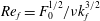 $Re_{f}=F_{0}^{1/2}/\unicode[STIX]{x1D708}k_{f}^{3/2}$
and
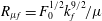 $R_{\unicode[STIX]{x1D707}f}=F_{0}^{1/2}k_{f}^{9/2}/\unicode[STIX]{x1D707}$
. For the constant energy injection rate runs of (2.10) we define
 $Re_{f}=I_{0}^{1/3}/\unicode[STIX]{x1D708}k_{f}^{4/3}$
and
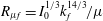 $R_{\unicode[STIX]{x1D707}f}=I_{0}^{1/3}k_{f}^{14/3}/\unicode[STIX]{x1D707}$
.
Equations (2.4) and (2.5) were solved using a standard parallel pseudo-spectral code with a fourth-order Runge–Kutta scheme for time integration and a two-thirds dealiasing rule. More details on the parallelization can be found in Gomez, Mininni & Dmitruk (Reference Gomez, Mininni and Dmitruk2005). All runs started from random initial conditions and were carried out long enough so that a statistically steady state was reached. All measurements and averages were made at this state unless otherwise stated. The resolutions used varied from
 $512^{2}$
to
 $4096^{2}$
grid points.
Our goal is to investigate how the system transitions to and from a bidirectional cascade as
 $Q$
is varied in the limit of large box size
 $L$
(or large-scale separation
 $L\gg 1/k_{f}$
) and large Reynolds numbers. Thus, close to the points of criticality, a series of runs were performed varying the parameter
 $Q$
for fixed values of
 $k_{f}L$
and
 $Re_{f}$
. Then the same series of runs were repeated for larger values of
 $k_{f}L$
or
 $Re_{f}$
until we observed convergence. The runs were separated into three cases: A, B, and C. See table 1 for a list of our cases and their corresponding parameters. Cases A and B investigated the transition from a purely forward cascade to a bidirectional cascade, with a constant forcing amplitude (2.9) and a constant energy injection rate (2.10), respectively. For these runs we fixed
 $Re_{f}$
while varying
 $k_{f}L$
, and measured the inverse energy cascade (which we expected to transition from being zero to being non-zero) via
 $\unicode[STIX]{x1D716}_{2D}^{-}/I$
. Finally, Case C investigated the transition from a bidirectional cascade to a purely inverse energy cascade. For these runs we fixed
 $k_{f}L$
, varied
 $Re_{f}$
, and measured the forward energy cascade (which we expected to transition from being non-zero to zero) via
 $\unicode[STIX]{x1D716}_{3D}^{+}/I$
.
A summary of the parameter ranges used in our simulations.

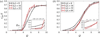
(a) Runs from Case A. Measure of the inverse cascade for various runs as we increased the box size
 $k_{f}L$
. Our runs converge to a sharp transition in the large box limit, confirming the existence of
 $Q_{3D}$
. The dashed vertical line represents the approximate value of
 $Q_{3D}$
. (b) Runs from Case B. A similar tendency is seen, although convergence is not yet reached.

3 Transition from a forward to a bidirectional cascade
We first investigate the first critical point
 $Q_{3D}$
that marks the transition from a forward cascade to bidirectional cascade. Figure 2 shows the dependence of the inverse cascade measured by the ratio of
 $\unicode[STIX]{x1D716}_{2D}^{-}/I$
as a function of
 $Q$
for flows driven by the deterministic forcing (2.9) in panel (a) and by constant injection of energy forcing (2.10) in panel (b). Since both cases are similar, we focus on panel (a), Case A. The three lines correspond to three different box sizes
 $k_{f}L$
as marked in the legend. For the smallest box size
 $k_{f}L=8$
the transition appears smooth with the presence of an inverse cascade at even the smallest values of
 $Q$
displayed. As the box size is increased the transition appears to become sharper, and at the largest box size the system seems to converge into a critical transition at the value
 $Q=Q_{3D}\simeq 3.6$
. Close to the critical point the inverse cascade
 $\unicode[STIX]{x1D716}_{2D}^{-}/I$
appears to scale linearly with the deviation from criticality
 $\unicode[STIX]{x1D716}_{2D}^{-}\propto (Q-Q_{3D})I$
for
 $Q>Q_{3D}$
. Looking at Case B in figure 2(b), the transition seems to take longer to converge but the same tendency is seen. For large values of
 $Q$
the curves saturate to a value slightly smaller than unity, which reflects that there is still a finite value of energy that is dissipated by viscous effects. This is because only moderate values of
 $Re$
are used. We discuss this issue more in the next section where the second critical point is investigated and
 $Re$
is varied.
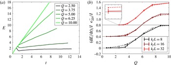
An alternative way to quantify the rate at which energy cascades towards the large scales is by measuring the rate of increase of energy. An inverse cascading system without large-scale dissipation and with a constant energy injection rate is expected to lead to a linear increase of energy with time. This linear increase is expected after a short transient time where small scales reach a quasi-steady state and before the largest scales of the system are exited and a condensate starts to form. The growth rate of the energy (i.e. the linear slope) is due to the inverse cascade and is equal to the inverse energy flux. We tested this method of measurement by performing runs identical to those of Case B (using the forcing with constant energy injection given in (2.10)) but this time without a hypo-dissipation term,
 $\unicode[STIX]{x1D707}=0$
. The energy evolution for the runs without hypo-dissipation are depicted in figure 3(a) for different values of
 $Q$
, where a linear increase of energy can be seen. The slope of the linear growth of energy for different values of
 $Q$
and
 $k_{f}L$
is calculated. These results are compared with the results obtained from steady-state runs in the presence of hypo-dissipation and are shown in figure 3(b) for three different values of the box size. For the smallest value of
 $k_{f}L$
the two measurements differ quite a bit, with the steady-state hypo-viscous simulations (dashed) which display a much more smooth behaviour, and the
 $\unicode[STIX]{x1D707}=0$
runs (solid) having significantly larger error. As the box size is increased the two methods of measuring the amplitude of the inverse cascade converge and the two curves overlap. Although measuring the inverse cascade by the slope of the energy versus time graph converges faster to the large box limit, the calculation using the hypo-dissipation term leads to much smaller error bars due to the long-time averaging that is possible in this case. The smaller error is favourable when attempting to determine very small trends of inverse cascade, as is seen figure 2.
(a) The evolution of the energy for different values of
 $Q$
in the absence of large-scale dissipation. (b) The results of our constant energy injection runs, comparing the two methods of measuring the inverse cascade. The solid lines represent the slope measurement with no hypo-dissipation, whereas the dashed lines represent the steady-state long-time-averaged measurements of runs with hypo-dissipation (Case B). The plots are shifted to emphasize differences. The horizontal black lines all correspond to
 $\unicode[STIX]{x1D716}_{2D}^{-}=0$
for the corresponding plot.

We next look how the spectral distribution of energy is changing as
 $Q$
is varied by looking at the energy spectra
 $E(k),E_{2D}(k),$
and
 $E_{q}(k)$
defined as:
 $$\begin{eqnarray}\displaystyle & \displaystyle E_{2D}(k)=\frac{1}{2}\mathop{\sum }_{k<|\boldsymbol{k}|\leqslant k+1}|\tilde{\boldsymbol{u}}_{2D}(\boldsymbol{k})|^{2}, & \displaystyle\end{eqnarray}$$
 $$\begin{eqnarray}\displaystyle & \displaystyle E_{q}(k)=\frac{1}{4}\mathop{\sum }_{k<|\boldsymbol{k}|\leqslant k+1}|\tilde{\boldsymbol{v}}_{q}(\boldsymbol{k})|^{2}, & \displaystyle\end{eqnarray}$$
where
 $\tilde{\boldsymbol{u}}_{2D}(\boldsymbol{k})$
and
 $\tilde{\boldsymbol{v}}_{q}(\boldsymbol{k})$
stand for the Fourier mode amplitude of wavenumber
 $\boldsymbol{k}$
of the
 $\boldsymbol{u}_{2D}$
and
 $\boldsymbol{v}_{q}$
fields respectively. The total energy spectrum
 $E(k)=E_{2D}(k)+E_{q}(k)$
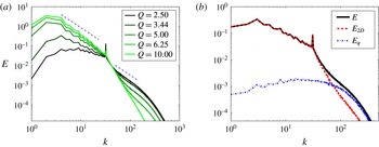
is shown in figure 4(a) for different values of
 $Q$
and for
 $k_{f}L=32$
. These spectra were outputted during the run time of our simulations and then afterwards averaged together during the steady-state period to get the final results. The smaller values of
 $Q$
are displayed with darker colours while the larger values of
 $Q$
are displayed with lighter colours. Clearly as
 $Q$
is increased there is more energy in the large scales and less energy in the small scales. For small values of
 $Q$
the energy spectrum is close to flat at the large scales
 $k<k_{f}$
and at the small scales
 $k>k_{f}$
it is compatible with a
 $k^{-5/3}$
power-law scaling. As we increase
 $Q$
the large scales gain more and more energy until we reach the point where a spectrum compatible with
 $k^{-5/3}$
is observed at the large scales
 $k<k_{f}$
, and at small scales the spectrum is very steep (steeper than
 $k^{-3}$
that is predicted for 2-D turbulence). This very steep behaviour is due to the small value of the Reynolds number used. The
 $k^{-3}$
spectrum is only realized in very high
 $Re$
(see Boffetta & Musacchio Reference Boffetta and Musacchio2010), and such values are beyond the scope of this work. Figure 4(b) compares the three spectra
 $E_{q}$
(blue, vertical dashed line) and
 $E_{2D}$
(red, dashed line) for the intermediate value of
 $Q=3.44>Q_{3D}$
. At large wavenumbers the energy spectrum is dominated by
 $E_{q}$
, while at small wavenumbers, which exhibit some inverse cascade, the spectrum is dominated by
 $E_{2D}$
.
(a) Spectra of the total energy for different values of
 $Q$
(averaged over many outputs). The colour of the curves become lighter and lighter as we have more and more inverse cascade. (b) The total energy
 $E(k)$
(black), the 2-D energy
 $E_{2D}$
(red) and the 3-D energy
 $E_{q}$
(blue) for
 $Q=3.44$
.

The direction of the cascade is best described by the direct measurement of the transfer of energy among scales provided by the nonlinear terms in our equations. More precisely, this flux of energy expresses the rate energy is transferred out of a given set of wavenumbers due to the nonlinearities. By performing a filtering of the 2-D velocity field
 $\boldsymbol{u}_{2D}$
and the 3-D velocity field
 $\boldsymbol{u}_{q}$
in Fourier space so that only the wavenumbers with modulus smaller than
 $k$
are kept, denoted by
 $\boldsymbol{u}_{2D}^{{<}k}$
and
 $\boldsymbol{u}_{q}^{{<}k}$
, one looks at only the structures of scales larger than
 $\ell =2\unicode[STIX]{x03C0}/k$
. With these filtered velocity one can calculate the flux of energy, defined to be:
 $$\begin{eqnarray}\displaystyle & \displaystyle \unicode[STIX]{x1D6F1}_{2D}(k)=-\langle \boldsymbol{u}_{2D}^{{<}k}\boldsymbol{\cdot }(\boldsymbol{u}_{2D}\boldsymbol{\cdot }\unicode[STIX]{x1D735}\boldsymbol{u}_{2D})\rangle , & \displaystyle\end{eqnarray}$$
 $$\begin{eqnarray}\displaystyle & \displaystyle \unicode[STIX]{x1D6F1}_{q}(k)=-\langle \boldsymbol{u}_{q}^{{<}k}\boldsymbol{\cdot }(\boldsymbol{u}_{2D}\boldsymbol{\cdot }\unicode[STIX]{x1D735}\boldsymbol{u}_{q})\rangle , & \displaystyle\end{eqnarray}$$
 $$\begin{eqnarray}\displaystyle & \displaystyle \unicode[STIX]{x1D6F1}_{T}(k)=-\langle \boldsymbol{u}_{2D}^{{<}k}\boldsymbol{\cdot }(\boldsymbol{u}_{q}\boldsymbol{\cdot }\unicode[STIX]{x1D735}\boldsymbol{u}_{q})\rangle -\langle \boldsymbol{u}_{q}^{{<}k}\boldsymbol{\cdot }(\boldsymbol{u}_{q}\boldsymbol{\cdot }\unicode[STIX]{x1D735}\boldsymbol{u}_{2D})\rangle . & \displaystyle\end{eqnarray}$$
The first flux
 $\unicode[STIX]{x1D6F1}_{2D}$
expresses the rate energy is transferred from large-scale
 $\boldsymbol{u}_{2D}$
modes to small-scale
 $\boldsymbol{u}_{2D}$
modes by self-interaction. The second flux
 $\unicode[STIX]{x1D6F1}_{q}$
expresses the rate energy is transferred from large-scale
 $\boldsymbol{u}_{q}$
modes to small-scale
 $\boldsymbol{u}_{q}$
modes through interactions with the 2-D field
 $\boldsymbol{u}_{2D}$
. Finally, the last flux
 $\unicode[STIX]{x1D6F1}_{T}$
expresses the rate energy is transferred to the small scales by a simultaneous exchange of energy from one field to the other. The total energy flux is given by
 $$\begin{eqnarray}\unicode[STIX]{x1D6F1}_{E}(k)=\unicode[STIX]{x1D6F1}_{2D}(k)+\unicode[STIX]{x1D6F1}_{q}(k)+\unicode[STIX]{x1D6F1}_{T}(k).\end{eqnarray}$$
In the inertial range
 $\unicode[STIX]{x1D6F1}_{E}(k)$
is constant and positive if the cascade is forward and constant and negative if the cascade is inverse. In the case for which
 $\boldsymbol{u}_{q}=0$
and enstrophy is conserved we can also define the flux of enstrophy as
 $$\begin{eqnarray}\unicode[STIX]{x1D6F1}_{\unicode[STIX]{x1D6FA}}(k)=-\langle \unicode[STIX]{x1D735}\times \boldsymbol{u}_{2D}^{{<}k}\boldsymbol{\cdot }(\boldsymbol{u}_{2D}\boldsymbol{\cdot }\unicode[STIX]{x1D735}(\unicode[STIX]{x1D735}\times \boldsymbol{u}_{2D}))\rangle .\end{eqnarray}$$
We note however that if
 $\boldsymbol{u}_{q}$
is not exactly zero the enstrophy flux
 $\unicode[STIX]{x1D6F1}_{\unicode[STIX]{x1D6FA}}(k)$
is not constant due to the enstrophy generation by the vorticity stretching term
 $\overline{\boldsymbol{u}_{q}\boldsymbol{\cdot }\unicode[STIX]{x1D735}\boldsymbol{u}_{q}}$
.
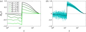
Figure 5 shows the time-averaged total energy flux
 $\unicode[STIX]{x1D6F1}_{E}$
normalized by the energy injection rate
 $I$
for different values of
 $Q$
. As before, dark lines correspond to small values of
 $Q$
while light lines correspond to larger values of
 $Q$
. For the smallest value of
 $Q$
the flux
 $\unicode[STIX]{x1D6F1}_{E}$
is almost zero for
 $k<k_{f}$
and positive for
 $k>k_{f}$
describing a unidirectional forward cascade. As
 $Q$
is increased a bidirectional cascade appears with both positive and negative fluxes in either side of the forcing wavenumber indicating that energy cascades to both large and small scales. At the largest value of
 $Q$
almost all energy cascades inversely demonstrated by the negative values of the flux for
 $k<k_{f}$
and almost zero values for
 $k>k_{f}$
. The time-averaged flux shows the predicted constant-in-
 $k$
behaviour for small
 $k$
while it is affected by viscosity in the large scales and thus decays with
 $k$
. Instantaneous fluxes however are strongly fluctuating. This is displayed in figure 5(b), where the time-averaged value of the flux (thick black line) is displayed along with numerous instantaneous fluxes (cyan lines) for the case of
 $Q=3.75$
. The role of the fluctuations becomes particular important close to the transition where the amplitude of the fluctuations becomes much larger than the mean value.
(a) The total energy flux
 $\unicode[STIX]{x1D6F1}_{E}$
for different values of
 $Q$
(averaged over many outputs). The lighter the shade of green, the higher the value of
 $Q$
. (b) For the case of
 $Q=3.75$
: The cyan/light blue lines show the instantaneous values of the total energy flux; the solid black line is their average, corresponding to one of the curves on (a).

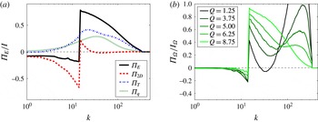
To demonstrate the role of each field in the cascade of energy we show, in figure 6(a), the decomposition of the total energy flux
 $\unicode[STIX]{x1D6F1}_{E}$
into the three components
 $\unicode[STIX]{x1D6F1}_{2D},\unicode[STIX]{x1D6F1}_{q}$
and
 $\unicode[STIX]{x1D6F1}_{T}$
for the value of
 $Q=3.75$
. The flux
 $\unicode[STIX]{x1D6F1}_{2D}$
is negative for all values of
 $k<k_{f}$
while it is positive but small for
 $k>k_{f}$
. The remaining fluxes
 $\unicode[STIX]{x1D6F1}_{q}$
and
 $\unicode[STIX]{x1D6F1}_{T}$
are positive for all
 $k$
. Thus the inverse cascade is driven by the
 $\unicode[STIX]{x1D6F1}_{2D}$
term whereas the forward cascade is driven mostly by
 $\unicode[STIX]{x1D6F1}_{q}$
and
 $\unicode[STIX]{x1D6F1}_{T}$
. It is worth noting that neither of these partial fluxes is constant in either inertial range. Furthermore
 $\unicode[STIX]{x1D6F1}_{q}$
and
 $\unicode[STIX]{x1D6F1}_{T}$
are positive and finite for
 $k<k_{f}$
implying that part of the energy transferred to the large scales by the
 $\boldsymbol{u}_{2D}$
field is brought back to the small scales by interactions with the
 $\boldsymbol{u}_{q}$
field. As
 $k$
is decreased the effect of
 $\unicode[STIX]{x1D6F1}_{q}$
and
 $\unicode[STIX]{x1D6F1}_{T}$
weakens and at the smallest
 $k$
only
 $\unicode[STIX]{x1D6F1}_{2D}$
remains non-zero.
Figure 6(b) shows the flux of enstrophy
 $\unicode[STIX]{x1D6F1}_{\unicode[STIX]{x1D6FA}}$
for different values of
 $Q$
. As discussed in the previous section enstrophy is only conserved by the nonlinearities when
 $\boldsymbol{u}_{q}=0$
. For large values of
 $Q$
, for which
 $\boldsymbol{u}_{q}$
is small, we expect that enstrophy will be quasi-conserved and its flux will be positive and slowly varying. This is indeed observed in this figure for
 $Q=8.75$
, where the enstrophy flux is slowly decreasing due to viscous effects. For smaller values of
 $Q$
, however, the enstrophy flux becomes non-monotonic with a sharp increase close to the dissipation scales. This is due to the generation of enstrophy by the
 $\boldsymbol{u}_{q}$
field that leads to an excess of enstrophy that is transported to the small scales.
(a) For the case of
 $Q=3.75$
: the total energy flux is shown in the thick black line and the contributions from each nonlinear term are shown in the other coloured lines. Notice that
 $\unicode[STIX]{x1D6F1}_{2D}$
is the only one with a negative contribution. One should also note that the green dotted line, corresponding to the term
 $\unicode[STIX]{x1D6F1}_{q}$
, is always positive for all
 $Q$
examined but that the blue dash-dot line, corresponding to
 $\unicode[STIX]{x1D6F1}_{T}$
, can be both negative and positive depending on
 $Q$
and
 $k$
. (b) The enstrophy flux
 $\unicode[STIX]{x1D6F1}_{\unicode[STIX]{x1D6FA}}$
for different values of
 $Q$
(averaged over many outputs) normalized by the enstrophy injection rate
 $I_{\unicode[STIX]{x1D6FA}}=\langle \unicode[STIX]{x1D735}\times \boldsymbol{u}_{2D}\boldsymbol{\cdot }\unicode[STIX]{x1D735}\times \boldsymbol{F}\rangle _{T}$
. The colour of the curves becomes lighter and lighter as the value of
 $Q$
increases.

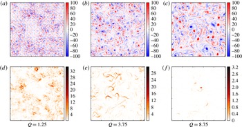
The results so far have demonstrated the presence of a bidirectional cascade in Fourier space. Further insight is obtained by looking at the resulting structures in physical space. Figure 7 shows, in (a–c), the 2-D vorticity
 $\unicode[STIX]{x1D735}\times \boldsymbol{u}_{2D}$
for three values of
 $Q$
. Panels (d–f) show the energy density
 ${\mathcal{E}}_{q}\equiv |\boldsymbol{v}_{q}|^{2}/4$
of the 3-D field at the same instant of time as the vorticity for the same values of
 $Q$
. The vorticity snapshots show that, as
 $Q$
is varied from small to large values, the structures change from small scale to structures larger than the forcing scale
 $k_{f}L=16$
, further demonstrating the growth of the inverse cascade as
 $Q$
is increased. For the smallest value of
 $Q$
the structures are small compared to the forcing scale, and one can notice by the sharp changes from blue to red that there are also large gradients of vorticity. For the largest value of
 $Q$
the flow has very similar structure to that obtained in pure 2-D simulations, where structures grow in size due to vortex clustering and stretching of the iso-vorticity lines (Chen et al.
Reference Chen, Ecke, Eyink, Rivera, Wan and Xiao2006; Eyink Reference Eyink2006; Xiao et al.
Reference Xiao, Wan, Chen and Eyink2009; Boffetta & Musacchio Reference Boffetta and Musacchio2010; Boffetta & Ecke Reference Boffetta and Ecke2012). Finally, the intermediate value of
 $Q$
appears to have characteristics of both extreme cases but concentrated in different regions of space. Some regions in space resemble the small-scale eddies and large gradient case of small
 $Q$
while other regions have the typical 2-D eddy structures. The structures in the 3-D energy density snapshots, shown in figure 7(d–f) are filamentary and are well correlated with the areas of high strain in the 2-D field. Furthermore, the density of these areas of high
 ${\mathcal{E}}_{q}$
appears to decrease with
 $Q$
. Combining these observations, one notices that, for small values of
 $Q$
, the intensity of vorticity is not uniform throughout the domain – some regions appear to be ‘3-D active’ and some regions to be ‘3-D quiet’. As
 $Q$
is increased the ‘3-D active’ regions appear to become less space filling. A similar behaviour has been observed in the transition from forward to inverse cascade in 2-D magnetohydrodynamic flows, where the role of
 $\boldsymbol{u}_{q}$
was played by the magnetic field (Seshasayanan et al.
Reference Seshasayanan, Benavides and Alexakis2014; Seshasayanan & Alexakis Reference Seshasayanan and Alexakis2016). This behaviour, as we will discuss next, has direct consequences for the behaviour of the flow close to the second critical point.
The 2-D vorticity
 $\unicode[STIX]{x1D735}\times \boldsymbol{u}_{2D}$
(a–c) and 3-D energy density
 ${\mathcal{E}}_{q}$
(d–f), for three values of
 $Q$
. The box size
 $k_{f}L=16$
is fixed for all cases. The grid pattern which is seen in (a) is due to the forcing.

4 Transition from a bidirectional to an inverse cascade
We now focus on large values of
 $Q$
for which the flow transitions from a bidirectional cascade to an inverse unidirectional cascade. As shown in the previous section the terms that involve the 3-D field
 $\boldsymbol{u}_{q}$
are responsible for driving the forward cascade. In their absence we recover the 2-D Navier–Stokes equation that leads to an inverse cascade with all energy dissipated at large scales in the large
 $Re$
limit. Thus in order to transition to a unidirectional inverse cascade the flow needs to become purely two-dimensional with
 $\boldsymbol{u}_{q}=0$
. This is indeed possible since a purely 2-D flow is always a solution of the 3-D Navier–Stokes equation, equation (2.1). Therefore if the initial data are exactly two-dimensional the flow will remain two-dimensional for all times cascading energy inversely. However these solutions can be unstable and small perturbations can grow exponentially driving the flow away from the 2-D behaviour and thus alter the direction of cascade. This brings us to the intuitive understanding of the second critical point. The bidirectional cascade will transition to a unidirectional inverse cascade when the layer thickness is so small (
 $Q$
is large enough) that all 3-D perturbations are damped and decay exponentially in time, and thus the 2-D solution is an attractor of the system. This is expected to occur when the thickness of the box
 $H_{2D}$
is such that the viscous dumping rate
 $\unicode[STIX]{x1D708}/H_{2D}^{2}$
due to the vertical variation alone is similar to the shear rate
 $u_{f}k_{f}$
that drives the 3-D instability. This argument
 $\unicode[STIX]{x1D708}/H_{2D}^{2}\sim u_{f}k_{f}$
implies that the second critical point
 $Q_{2D}$
will satisfy:
 $$\begin{eqnarray}Q_{2D}=\unicode[STIX]{x03C0}/(H_{2D}k_{f})\propto \sqrt{Re}.\end{eqnarray}$$
A more precise estimate for the location of
 $Q_{2D}$
can be obtained by looking at the energy evolution of the 3-D component of the flow that reads
 $$\begin{eqnarray}\frac{1}{2}\frac{\text{d}}{\text{d}t}\langle |\boldsymbol{u}_{q}|^{2}\rangle =-\langle \boldsymbol{u}_{q}\boldsymbol{\cdot }(\unicode[STIX]{x1D735}\boldsymbol{u}_{2D})\boldsymbol{\cdot }\boldsymbol{u}_{q}\rangle -\unicode[STIX]{x1D708}\langle |\unicode[STIX]{x1D735}\boldsymbol{u}_{q}|^{2}\rangle \equiv {\mathcal{H}}.\end{eqnarray}$$
Note that the equation above is also valid for the full Navier–Stokes equations, not just our model, with
 $\boldsymbol{u}_{q}=\boldsymbol{u}-\boldsymbol{u}_{2D}$
. The 2-D solutions will be globally stable if the functional
 ${\mathcal{H}}$
is negative definite in which case all 3-D perturbations will decay independent of the initial conditions. We can prove that this is the case for a given range of
 $Q$
using the following rigorous inequalities. Using Hölder’s inequality the vortex stretching term
 $\langle \boldsymbol{u}_{q}\boldsymbol{\cdot }(\unicode[STIX]{x1D735}\boldsymbol{u}_{2D})\boldsymbol{\cdot }\boldsymbol{u}_{q}\rangle$
is bounded by
 $$\begin{eqnarray}|\langle \boldsymbol{u}_{q}\boldsymbol{\cdot }(\unicode[STIX]{x1D735}\boldsymbol{u}_{2D})\boldsymbol{\cdot }\boldsymbol{u}_{q}\rangle |\leqslant \Vert \unicode[STIX]{x1D735}\boldsymbol{u}_{2D}\Vert _{\infty }\langle |\boldsymbol{u}_{q}|^{2}\rangle ,\end{eqnarray}$$
where
 $\Vert \unicode[STIX]{x1D735}\boldsymbol{u}_{2D}\Vert _{\infty }$
stands for the
 $L_{\infty }$
norm (both in time and space) of the gradient of
 $\boldsymbol{u}_{2D}$
. Furthermore Poincaré’s inequality gives, for the dissipation term, that
 $\langle |\unicode[STIX]{x1D735}\boldsymbol{u}_{q}|^{2}\rangle \geqslant \unicode[STIX]{x1D708}q^{2}\langle |\boldsymbol{u}_{q}|^{2}\rangle$
. These two results lead to the negativity of
 ${\mathcal{H}}$
if
 $Q^{2}=q^{2}/k_{f}^{2}\geqslant \Vert \unicode[STIX]{x1D735}\boldsymbol{u}_{2D}\Vert _{\infty }/k_{f}^{2}\unicode[STIX]{x1D708}$
. Provided that
 $\Vert \unicode[STIX]{x1D735}\boldsymbol{u}_{2D}\Vert _{\infty }$
is bounded, this result guarantees that, beyond some value of
 $Q$
, the flow becomes exactly two-dimensional. However, deriving an upper bound on
 $\Vert \unicode[STIX]{x1D735}\boldsymbol{u}_{2D}\Vert _{\infty }$
in terms of the control parameters of the system is not trivial. An upper bound on the long-time-averaged growth rate of
 $\langle |\boldsymbol{u}_{q}|^{2}\rangle$
was derived in Gallet & Doering (Reference Gallet and Doering2015) where the two-dimensionalization of a flow due to the presence of an external strong magnetic field
 $B_{0}$
was examined. Their results extend directly to our case by setting
 $B_{0}=0$
. They were able to show, using properties of the steady-state 2-D Navier–Stokes equations (Alexakis & Doering Reference Alexakis and Doering2006), that the 3-D energy will decay, in the long-time limit if
 $Q$
satisfies:
 $$\begin{eqnarray}Q^{2}\geqslant Re^{3}\left(\frac{c_{1}}{Re}+c_{2}\right),\end{eqnarray}$$
where each
 $c_{i}$
is a positive dimensionless number that depends on forcing shape and other non-universal properties of the flow and
 $Re$
is based on the r.m.s. velocity of the flow. Note that
 $Q$
does not scale as we predicted with respect to
 $Re$
. This is because this bound is very conservative and does not capture all the physics at the transition point. However, despite this loose scaling, this results guarantees that the transition from a bidirectional to a purely inverse cascade will be through a critical point because it guarantees that there is a value of
 $Q$
above which
 $\unicode[STIX]{x1D716}_{3D}^{+}$
is exactly zero.
Another less conservative bound which was derived in Gallet & Doering (Reference Gallet and Doering2015) is based on the linear stability analysis of 2-D flows to 3-D perturbations. Linear stability guarantees that the 2-D solutions are locally stable but does not exclude the possibility that a locally attracting 3-D solution also exist for the same parameters. Their analysis shows that 2-D solutions (for harmonic forcing and in the absence of hypo-dissipation term) are linearly stable provided that
 $$\begin{eqnarray}Q^{2}\geqslant Re\left(c_{3}+c_{4}\ln |Re|+c_{5}\ln \left|\frac{k_{f}}{2\unicode[STIX]{x03C0}}\right|\right).\end{eqnarray}$$
Up to logarithmic corrections this result follows the scaling
 $Q_{2D}\sim Re^{1/2}$
, which is what our scale analysis predicts.
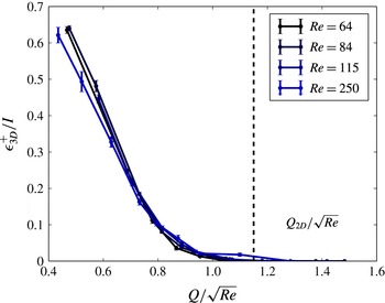
Run set C.
 $\unicode[STIX]{x1D716}_{3D}^{+}$
normalized by the energy injection rate for various runs as we increased the Reynolds number. Rescaling
 $Q$
by our scale analysis prediction collapses the curves into one. The dashed vertical line represents the approximate value of
 $Q_{2D}$
, after which all runs have decaying 3-D energy.

This scaling is clearly demonstrated by our numerical simulations in figure 8 that shows the energy dissipation rate
 $\unicode[STIX]{x1D716}_{3D}^{+}$
as a function of the rescaled
 $Q/\sqrt{Re}$
. This rescaling of
 $Q$
collapses the curves together. The vertical dashed line marks the critical value
 $Q_{2D}=C_{2D}\sqrt{Re}$
(where
 $C_{2D}\simeq 1.16$
) and represents the point after which the amplitude of the 3-D field decays exponentially. In the absence of
 $\boldsymbol{u}_{q}$
we have a 2-D solution –
 $\unicode[STIX]{x1D716}_{3D}^{+}$
is zero and most of the energy is dissipated in the large scales. Note that for a given value of
 $Q$
the exact two-dimensionalization occurs for the values of
 $Re$
in the range
 $Re\leqslant Q^{2}/C_{2D}^{2}$
. Since
 $Re$
is bounded from above there is always some viscous dissipation
 $\unicode[STIX]{x1D716}_{2D}^{+}$
. Thus, a strict inverse cascade where all the injected energy is dissipated at the large scales
 $\unicode[STIX]{x1D716}_{2D}^{-}=I_{0}$
and
 $\unicode[STIX]{x1D716}_{2D}^{+}+\unicode[STIX]{x1D716}_{3D}^{+}=0$
is realized only in the limit
 $Re\rightarrow \infty$
,
 $Q\rightarrow \infty$
with
 $Q\geqslant Q_{2D}=C_{2D}Re^{1/2}$
. On the other hand the small-scale dissipation due to the
 $\boldsymbol{u}_{q}$
field
 $\unicode[STIX]{x1D716}_{3D}^{+}$
becomes exactly zero
 $\unicode[STIX]{x1D716}_{3D}^{+}=0$
for any finite value of
 $Re$
that satisfies
 $Re\leqslant Q^{2}/C_{2D}^{2}$
. It is also worth pointing out that the dependence of
 $\unicode[STIX]{x1D716}_{3D}^{+}$
on the deviation from criticality differs from that of
 $\unicode[STIX]{x1D716}_{2D}^{-}$
close to the first critical point
 $Q_{3D}$
that was linear. Close to
 $Q_{2D}$
the energy dissipation
 $\unicode[STIX]{x1D716}_{3D}^{+}$
follows the relation
 $$\begin{eqnarray}\unicode[STIX]{x1D716}_{3D}^{+}\propto (Q_{2D}-Q)^{\unicode[STIX]{x1D6FD}}I,\quad \text{where }\unicode[STIX]{x1D6FD}>1\text{ and }Q\leqslant Q_{2D}.\end{eqnarray}$$
The exponent
 $\unicode[STIX]{x1D6FD}$
was found to be close to
 $\unicode[STIX]{x1D6FD}\simeq 2$
. To understand the origin of this exponent we need to look at the temporal and spatial form of the unstable field
 $\boldsymbol{u}_{q}$
.
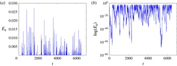
A typical time series of the 3-D energy for a
 $Q$
very close to
 $Q_{2D}$
. (a) Shows linear scalings and the typical picture of an on–off intermittent signal, whereas (b) shows the same signal but in log–linear scale.

Figure 9 shows a typical signal for the evolution of the energy of the 3-D field
 $\boldsymbol{u}_{q}$
as a function of time, in linear (a) and log-linear (b) scale. The signal exhibits bursts of energy followed by times with very weak energy. This is a signature of ‘on–off’ intermittency. On–off intermittency is a generic behaviour that appears in the vicinity of an instability in the presence of multiplicative noise (Fujisaka et al.
Reference Fujisaka, Ishii, Inoue and Yamada1986; Platt, Spiegel & Tresser Reference Platt, Spiegel and Tresser1993). It has been observed in turbulent dynamo simulations (Alexakis & Ponty Reference Alexakis and Ponty2008), in electronic circuits (Hammer et al.
Reference Hammer, Platt, Hammel, Heagy and Lee1994), in electrohydrodynamic convection (John, Stannarius & Behn Reference John, Stannarius and Behn1999) and spin-wave systems (Rödelsperger, Čenys & Benner Reference Rödelsperger, Čenys and Benner1995). In such situations the unstable modes have a growth rate that varies strongly with time, taking both positive and negative values. Our system also falls in this category because for small values of
 $\boldsymbol{u}_{q}$
it is linearly advected by a turbulent/chaotic flow
 $\boldsymbol{u}_{2D}$
. Thus, at some instances of time
 $\boldsymbol{u}_{2D}$
is efficient at exponentially increasing
 $\boldsymbol{u}_{q}$
while at others
 $\boldsymbol{u}_{q}$
is exponentially decreased. In its simplest form on–off intermittency models a single mode
 $X$
that is amplified or decreased by a fluctuating growth rate
 $\unicode[STIX]{x1D6FC}+\unicode[STIX]{x1D709}$
and is restricted from taking very large values by a nonlinearity
 $-X^{3}$
:
 $$\begin{eqnarray}{\dot{X}}=(\unicode[STIX]{x1D6FC}+\unicode[STIX]{x1D709})X-X^{3}.\end{eqnarray}$$
Here
 $\unicode[STIX]{x1D6FC}$
represents mean growth rate and
 $\unicode[STIX]{x1D709}$
represents a zero mean random noise. In the thin layer turbulent system the 3-D instabilities of the 2-D flow, whose energy is described by (4.2), have an averaged growth rate
 $\unicode[STIX]{x1D6FC}$
that is proportional to the deviation from criticality
 $\unicode[STIX]{x1D6FC}\propto (Q_{2D}-Q)$
. At the same time the role of the turbulent fluctuations of the 2-D field
 $\boldsymbol{u}_{2D}$
is played by the random multiplicative noise. If the averaged growth rate
 $\unicode[STIX]{x1D6FC}$
in (4.7) is sufficiently smaller than the fluctuations
 $\unicode[STIX]{x1D709}$
of the instantaneous growth rate, then the system spends long intervals of time with very small amplitudes (off phase) intervened by short burst where the nonlinearities are effective (on phases). In log scale the amplitude of the unstable mode follows a biased random walk bounded from above by the nonlinearities. The model predicts that, close to the onset, the probability distribution function (PDF)
 $P(E_{q})$
of the energy of the mode
 $E_{q}\sim X^{2}$
follows the scaling
 $$\begin{eqnarray}P(E_{q})\sim E_{q}^{\unicode[STIX]{x1D6FC}/D-1},\quad \text{for}~X\ll 1,\end{eqnarray}$$
where
 $D$
is the amplitude of the noise. Furthermore, the duration of the off phases
 $T_{off}$
diverges with the deviation from the onset (here
 $Q_{2D}-Q$
) as
 $T_{off}\propto (Q_{2D}-Q)^{-1}$
while the amplitude
 $E_{on}$
and the time
 $T_{on}$
in the on phase becomes independent of (
 $Q_{2D}-Q$
). This implies that the time-averaged energy scales like
 $$\begin{eqnarray}\langle {\mathcal{E}}_{q}\rangle _{T}\propto \frac{E_{on}T_{on}}{T_{off}+T_{on}}\propto Q_{2D}-Q,\end{eqnarray}$$
where
 $\langle {\mathcal{E}}_{q}\rangle _{T}$
is also the time average of
 $E_{q}$
. Note that this is not the behaviour we observe in figure 8, which suggests a scaling closer to
 $\langle {\mathcal{E}}_{q}\rangle _{T}\propto (Q_{2D}-Q)^{2}$
, since the time averaged
 $\unicode[STIX]{x1D716}_{3D}^{+}$
is proportional to the time average of
 $E_{q}$
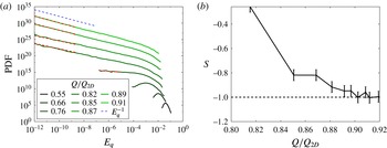
. Figure 10(a) shows the PDF of the energy
 $E_{q}$
calculated for different values of
 $Q$
. In agreement with the model when the critical value
 $Q_{2D}$
is approached, the PDF becomes singular showing a power-law behaviour
 $P(E_{q})\propto (E_{q})^{S(Q)}$
. The exponents
 $S(Q)$
of this power law are shown in figure 10(b). As criticality is approached
 $Q\rightarrow Q_{2D}$
these exponents tend to
 $-1$
in agreement again with the model. However this asymptotic value is not approached linearly (i.e.
 $S(Q)\simeq (Q_{2D}-Q)/D-1$
) as the model suggests but closer to a quadratic behaviour
 $S(Q)\simeq (Q_{2D}-Q)^{2}/D^{2}-1$
. Thus, just as with the scaling observed in (4.6) there is a disagreement with this model.
(a) The PDF in time of
 $E_{q}$
. As before, dark means farther away from
 $Q_{2D}$
and thus smaller
 $Q$
and light green is the most two-dimensional (closest to
 $Q_{2D}$
). The blue dashed line represents
 $E_{q}^{-1}$
and the red dashed lines represent where the power-law exponent measurements were taken (if any). (b) Various values of the exponents
 $S(Q)$
versus the fraction
 $Q/Q_{2D}$
that measures the deviation from criticality. These values are the slopes of the red dashed lines in (a). Notice the approach to
 $-1$
, as the model predicts.

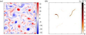
The vorticity
 $\unicode[STIX]{x1D735}\times \boldsymbol{u}_{2D}$
(a) and the 3-D energy density
 ${\mathcal{E}}_{q}$
(b) for a point
 $Q/Q_{2D}=0.92$
, right before
 $Q_{2D}$
. For
 $k_{f}L=8$
and constant forcing amplitude. Note the very localized structure of the 3-D energy, an extreme of a trend seen in figure 7.

Resolution comes from looking at the spatial behaviour of the unstable modes. Figure 11 shows a snapshot of the vorticity
 $\unicode[STIX]{x1D735}\times \boldsymbol{u}_{2D}$
in panel (a) and of the 3-D energy density
 ${\mathcal{E}}_{q}=|\boldsymbol{v}_{q}|^{2}/4$
in panel (b). The vorticity shows the classical behaviour of 2-D turbulence. The 3-D energy, however, shows a very intermittent behaviour in space: most of the 3-D energy is concentrated in a single structure occupying a small fraction of the area of the domain size. Comparing with figure 7(d–f) we see that, as
 $Q$
is increased and
 $Q_{2D}$
is approached, there are less and less 3-D structures occupying a smaller and smaller fraction of the domain area. For
 $Q$
really close to
 $Q_{2D}$
in figure 11(b) only a single structure or two exist. The unstable solution thus is not only intermittent in time, but it is also intermittent in space!
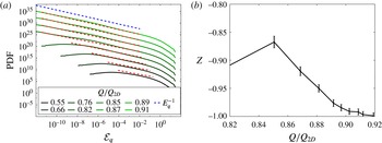
(a) The PDF in space of
 ${\mathcal{E}}_{q}$
. As before, dark means farther away from
 $Q_{2D}$
and thus smaller
 $Q$
and light green is the most two-dimensional (closest to
 $Q_{2D}$
). The blue dashed line represents
 $E_{q}^{-1}$
and the red dashed lines represent where the measurements of the exponents were taken. (b) Various values of the measured power-law exponents
 $Z$
versus the fraction
 $Q/Q_{2D}$
. The measured power laws are demonstrated by the red dashed lines in (a).

Figure 12 shows the PDF in space of
 ${\mathcal{E}}_{q}$
measured for different values of
 $Q$
. Just like the PDF of the energy
 $E_{q}$
the PDF of
 ${\mathcal{E}}_{q}$
shows a power-law behaviour: as criticality is approached
 $P({\mathcal{E}}_{q})\propto {\mathcal{E}}_{q}^{Z}$
with
 $Z\rightarrow -1$
as
 $Q\rightarrow Q_{2D}$
. Spatial intermittency is not taken into account in the on–off intermittency model (4.7) that takes into account the evolution of only one single mode. In our system the nonlinearity (on phase) is not only visited rarely in time but also rarely in space. The averaged energy in space and time will then satisfy
 $$\begin{eqnarray}\langle {\mathcal{E}}_{q}^{n}\rangle _{T}=\frac{{\mathcal{E}}_{on}^{n}T_{on}V_{on}}{(T_{on}+T_{off})V},\end{eqnarray}$$
where
 $V_{on}$
is the area occupied by the ‘3-D active’ regions, and
 $V$
is the total area of our system. The scaling of
 $\langle {\mathcal{E}}_{q}^{n}\rangle _{T}$
on
 $(Q_{2D}-Q)$
will thus not only depend on the scaling of the time fraction
 $T_{on}/T_{off}$
but also on the area fraction
 $V_{on}/V_{off}$
. The model in (4.7) is not sufficient to describe our system and most likely an extended system with random multiplicative noise both in space and time will be required to capture correctly the statistics of our system (Grinstein, Munoz & Tu Reference Grinstein, Munoz and Tu1996; Horsthemke & Lefever Reference Horsthemke and Lefever2006). Such a possibility will be examined in future work.
5 Conclusions
In this work we investigated turbulence in a thin layer using numerical simulations of a two-dimensional model of the Navier–Stokes equation obtained by a severe Galerkin truncation in the vertical direction. The decreased dimensionality of our system allowed us to systematically investigate the transition from a forward to an inverse cascade. Our results demonstrate the existence of two critical heights (quantified by the parameter
 $Q$
) with an unexpectedly rich behaviour close to criticality.
The first critical height
 $H_{3D}=\ell _{f}/Q_{3D}$
marks the transition from a forward cascade for
 $H>H_{3D}$
to a bidirectional cascade for
 $H<H_{3D}$
. Above this critical height
 $H>H_{3D}$
the 3-D component of the flow is in equipartition with the 2-D part of the flow and the energy cascades to the small scales. Although there is some transfer of energy from
 $\boldsymbol{u}_{2D}$
to the large scales it is compensated by the forward transfer caused by the three-dimensional
 $\boldsymbol{u}_{q}$
field leading to zero net transfer of energy to the large scales. The spectrum displays a power law compatible with a Kolmogorov spectrum at large wavenumbers. The structures in this case are small-scale vortex tubes occupying a finite fraction of the computational domain.
Below but close to the critical height
 $H\lesssim H_{3D}$
a weak inverse cascade is observed. The amplitude of the inverse cascade displays a close to linear dependence with the deviation from criticality
 $Q-Q_{3D}$
(or
 $H_{3D}-H$
). The transfer of energy to the large scales from the two-dimensional field
 $\boldsymbol{u}_{2D}$
cannot be compensated by the forward transfer of the three-dimensional field
 $\boldsymbol{u}_{q}$
, which is weaker, leading to the observed inverse cascade. The spectrum is close to Kolmogorov
 $k^{-5/3}$
both at the large and the small scales. In real space one observes the coexistence of large-scale 2-D structures (similar to a pure 2-D flow) along with 3-D vortex tubes. The two distinct structures occupy different regions of space. The fraction of the area they occupy depends on the deviation from the onset. It is possible that the interactions of these 2-D vortices with the 3-D structures display predator–prey dynamics, as has been recently claimed for the transition to turbulence in Couette and Poiseuille flow (Barkley et al.
Reference Barkley, Song, Mukund, Lemoult, Avila and Hof2015; Goldenfeld & Shih Reference Goldenfeld and Shih2017; Lemoult et al.
Reference Lemoult, Shi, Avila, Jalikop, Avila and Hof2016; Sano & Tamai Reference Sano and Tamai2016), and thus this transition could also fall in the universality class of directed percolation (Obukhov Reference Obukhov1980) as suggested by Pomeau (Reference Pomeau1986) for subcritical instabilities in turbulence.
The second critical height
 $H_{2D}=\ell _{f}/Q_{2D}$
marks the transition from the bidirectional cascade for
 $H_{2D}<H<H_{3D}$
to an inverse cascade for
 $H<H_{2D}$
. The critical point
 $H_{2D}$
is shown to scale like
 $H_{2D}\propto \ell _{f}Re^{-1/2}$
. It can be shown that for all
 $H<H_{2D}$
all 3-D perturbations decay exponentially in time (Gallet & Doering Reference Gallet and Doering2015). For values of
 $H$
larger but close to
 $H_{2D}$
the three-dimensional flow exhibited a strongly intermittent behaviour. The total energy displayed on–off intermittency behaviour in time with bursts of energy. At the same time intermittent behaviour was also observed in space with the 3-D vortex-tube-like structures occupying a lesser domain area the closer
 $H$
is to
 $H_{2D}$
. This intermittent behaviour results from the almost linear evolution of the unstable 3-D mode
 $\boldsymbol{u}_{q}$
driven by the spatio-temporal fluctuations of the 2-D turbulence. The transition close to this point then could possibly modelled by extended systems in the presence of multiplicative noise (Grinstein et al.
Reference Grinstein, Munoz and Tu1996; Horsthemke & Lefever Reference Horsthemke and Lefever2006).
Our model was based on a drastic Galerkin truncation in the vertical direction so it is worth discussing the expected effect of including higher modes. Close to the critical point
 $Q_{2D}$
, since this is where the model is valid, we expect that it captures the transition quite accurately. At a neighbourhood of this point one can envision an expansion based on the distance from the onset
 $(Q_{2D}-Q)\ll 1$
so that only one
 $q$
-mode (the one with the smallest
 $q$
) is unstable. For the other critical point
 $Q_{3D}$
there might be some differences. For example the exact location of the critical point might change. We do not expect, however, to see any change with respect to the critical nature of this point because if one 3-D mode is sufficient to stop the inverse cascade, then certainly two or three modes will do even better. Of course this expectation remains to be seen by examining the full 3-D layer problem, something that is well beyond the purpose of this work.
The precise statistical description and the possible universality class of the two critical points certainly require further investigation. The present investigation however clearly demonstrated the non-triviality of the two critical points and their unexpectedly rich behaviour. Whether similar transitions are observed in other systems such as rotating, stratified or magnetized flows remains to be seen.
Acknowledgements
This work was granted access to the HPC resources of MesoPSL financed by the Region Ile de France and the project Equip@Meso (reference ANR-10-EQPX-29-01) of the programme Investissements d’Avenir supervised by the Agence Nationale pour la Recherche and the HPC resources of GENCI-TGCC-CURIE & GENCI-CINES-OCCIGEN (Project nos x2016056421 and x2017056421) where the present numerical simulations have been performed.