




No CrossRef data available.
DIAGNOSTIC CHECKING FOR THE ADEQUACY OF NONLINEAR TIME SERIES MODELS
Published online by Cambridge University Press: 24 September 2003
Abstract
We propose a new diagnostic test for linear and nonlinear time series models, using a generalized spectral approach. Under a wide class of time series models that includes autoregressive conditional heteroskedasticity (ARCH) and autoregressive conditional duration (ACD) models, the proposed test enjoys the appealing “nuisance-parameter-free” property in the sense that model parameter estimation uncertainty has no impact on the limit distribution of the test statistic. It is consistent against any type of pairwise serial dependence in the model standardized residuals and allows the choice of a proper lag order via data-driven methods. Moreover, the new test is asymptotically more efficient than the correlation integral–based test of Brock, Hsieh, and LeBaron (1991, Nonlinear Dynamics, Chaos, and Instability: Statistical Theory and Economic Evidence) and Brock, Dechert, Scheinkman, and LeBaron (1996, Econometric Reviews 15, 197–235), the well-known BDS test, against a class of plausible local alternatives (not including ARCH). A simulation study compares the finite-sample performance of the proposed test and the tests of BDS, Box and Pierce (1970, Journal of the American Statistical Association 65, 1509–1527), Ljung and Box (1978, Biometrika 65, 297–303), McLeod and Li (1983, Journal of Time Series Analysis 4, 269–273), and Li and Mak (1994, Journal of Time Series Analysis 15, 627–636). The new test has good power against a wide variety of stochastic and chaotic alternatives to the null models for conditional mean and conditional variance. It can play a valuable role in evaluating adequacy of linear and nonlinear time series models. An empirical application to the daily S&P 500 price index highlights the merits of our approach.We thank the co-editor (Don Andrews) and two referees for careful and constructive comments that have lead to significant improvement over an earlier version. We also thank C.W.J. Granger, D. Tjøstheim, and Z. Xiao for helpful comments. Hong's participation is supported by the National Science Foundation via NSF grant SES–0111769. Lee thanks the UCR Academic Senate for research support.
Information
- Type
- Research Article
- Information
- Copyright
- © 2003 Cambridge University Press
1. INTRODUCTION
The development of nonlinear time series analysis has been advancing rapidly (e.g., Subba Rao and Gabr, 1984; Priestley, 1988; Tong, 1990; Brock, Hsieh, and LeBaron, 1991; Granger and Teräsvirta, 1993; Tjøstheim, 1994; Teräsvirta, Tjøstheim, and Granger, 1994; Terdik, 1999). In modern time series analysis, one often considers the data generating process

where It−1 is the information set available at time t − 1 and {εt} is a sequence of independently and identically distributed (i.i.d.) innovations. Often, {εt} has mean 0 and variance 1 such that g0(It−1) = E(Yt|It−1) and h02(It−1) = var(Yt|It−1) almost surely (a.s.). For various examples that belong to class (1.1), see, e.g., Tong (1990) and Granger and Teräsvirta (1993). It is also possible that {εt} is an i.i.d. nonnegative sequence with E(εt) = 1. An example is the autoregressive conditional duration (ACD) process introduced in Engle and Russell (1998) for irregularly spaced time series, where g0(It−1) = 0 and h0(It−1) = E(Yt|It−1) is the conditional duration of the nonnegative time duration process {Yt}.
Various models for g0(·) and h0(·) have been proposed in the literature. Consider a model

where g(·,θ) and h(·,θ) are some known parametric specifications for g0(·) and h0(·), θ ∈ Θ is an unknown finite-dimensional parameter vector, and {et(θ)} is an unobservable series. Specification (1.2) covers most commonly used linear and nonlinear time series models. Examples include ACD, autoregressive conditional heteroskedasticity (ARCH), autoregressive moving average (ARMA), bilinear, nonlinear moving average, Markov regime-switching, smooth transition, exponential, and threshold autoregressive models. When g(·,θ) and h(·,θ) are correctly specified for g0(·) and h0(·), i.e., when there exists some θ0 ∈ Θ such that g(·,θ0) = g0(·) and h(·,θ0) = h0(·) a.s., the model standardized error series {et(θ0)} coincides with the true innovation series {εt} and therefore is i.i.d. In contrast, if g(·,θ) is inadequate for g0(·) and/or h(·,θ) is inadequate for h0(·), i.e., if there exists no θ ∈ Θ such that g(·,θ) = g0(·) and/or h(·,θ) = h0(·) a.s., {et(θ)} will be serially dependent for all θ ∈ Θ. Consequently, to test adequacy of model (1.2), one can check whether there exists some θ0 ∈ Θ such that {et(θ0)} is i.i.d. Tests for i.i.d. rather than for white noise are more suitable and useful in nonlinear time series analysis, in particular when higher order conditional moments or the conditional probability distribution are of interest (e.g., Brock et al., 1991; Brock, Dechert, Scheinkman, and LeBaron, 1996, Christoffersen, 1998; Diebold, Gunther, and Tay, 1998; Kim, Shephard, and Chib, 1998; Clement and Smith, 2000; Elerian, Chib, and Shephard, 2001). See also an empirical application in Section 8.
Because {et(θ0)} is unobservable, one has to use the standardized estimated residual

where

is a consistent estimator of θ0 based on a random sample {Yt}t=1n of size

is the observed information set available at period t that may involve certain initial values. To construct an asymptotically valid test procedure, it is important to examine whether and how the use of

rather than {et ≡ et(θ0)}t=1n affects the limit distribution of a test statistic, besides its power property (see Tjøstheim, 1996).
Often, the information set It−1 consists of lagged variables {Yt−j,j > 0}. When g0(It−1) is linear in It−1, Yt is called linear in conditional mean on It−1 (Lee, White, and Granger, 1993). If in addition h0(It−1) = σ a.s., {Yt} is called completely linear in It−1 (Granger, 2001; Granger and Lee, 1999). Assuming h0(It−1) = σ a.s. in an ARMA framework, Box and Pierce (1970) and Ljung and Box (1978) propose a diagnostic test for an ARMA(p0,q0) model:

where

is the sample autocorrelation function of

is an estimated ARMA(p0,q0) model. Here, {êt} is the usual estimated residuals because no conditional variance estimation is involved. The degrees of freedom of the Box–Pierce–Ljung (BPL) test depend on p0 + q0, the number of the estimated parameters. Hong (1996) and Paparoditis (2000a, 2000b) propose spectrum-based diagnostic tests that generalize the BPL(p) test.
It has been pointed out for a long time (e.g., Granger and Andersen, 1978; Granger, 1983) that the Box–Pierce–Ljung test has no power against nonlinear dependencies with zero autocorrelation, such as some bilinear and nonlinear moving-average (MA) processes. Using the sample autocorrelation function of squared residuals, McLeod and Li (1983) suggest a test for linearity against unspecified nonlinearity. For a null ARMA(p0,q0) model, the McLeod and Li (1983) test statistic is

where

is the sample autocorrelation function of

. This test has good power against ARCH. It also has power against departures from linearity that have apparent ARCH structures. The null limit distribution of the test statistic is a χp2 distribution; the degrees of freedom need not be adjusted when only an ARMA model is estimated. As pointed out in Granger and Teräsvirta (1993), ML(p) is asymptotically equivalent to the Lagrange multiplier test for ARCH of Engle (1982).
When testing the adequacy of an ARCH/generalized autoregressive moving average (GARCH) model, many researchers have applied the McLeod–Li test to the squares of the estimated standardized residuals.1
A partial list of the papers using this procedure, as given in Tse and Zuo (1997, p. 238), includes Bollerslev (1987), Hsieh (1989), Hamao, Masulis, and Ng (1990), Lee and Tse (1991), Cheung and Ng (1992), Higgins and Bera (1992), and Karolyi (1995).

where

is the sample autocorrelation function of

is an estimated ARCH(r) model. The null limit distribution depends on r, the order of the ARCH model. When other conditional variance models are estimated, the test statistic itself has to be modified as suggested by Li and Mak (1994) or by Lundbergh and Teräsvirta (2002).
Brock et al. (1991, 1996) propose a diagnostic test for model (1.2), using chaos theory:

where the sample correlation integral (cf. Grassberger and Procaccia, 1983)

1(·) is an indicator function, m is the so-called embedding dimension, d is a distance parameter, and

is an asymptotic variance estimator. The statistic

measures the fraction of pairs of histories

that are within distance d of each other. If

are close in value, so will be subsequent pairs for a chaotic process but not for an i.i.d. sequence. Thus, BDS(m,d) is expected to have good power against chaos. In addition, it also has power against a wide range of stochastic dependent processes. To see this, observe that when {et} is i.i.d., we have

for all positive integers m and all distances d > 0. In other words, the correlation integral Cm(d) behaves like the characteristic function of a serial string in the sense that the correlation integral of a serial string is the product of correlation integrals of component substrings. If Cm(d) ≠ C1(d)m, there is evidence against the i.i.d. hypothesis, and BDS will gain power.2
It should be emphasized, as correctly pointed out by one referee, that the BDS test is not a test for chaos against stochastic alternatives. This is the case because the test does not have chaos as the null hypothesis. Instead, the null hypothesis of the BDS test is i.i.d., and when it is rejected, chaos is just one of infinitely many possible reasons for the rejection.
As shown in Brock et al. (1991, Ch. 2 and Appendix D), BDS(m,d) has the appealing “nuisance-parameter-free” property that any n1/2-consistent parameter estimator

has no impact on its null limit distribution under a class of conditional mean models g(·,θ). This, together with good power against a wide range of dependent alternatives, has made BDS(m,d) a convenient and powerful diagnostic tool for nonlinear time series models. It has been recommended by Brock et al. (1991) as a portmanteau lack of fit test for nonlinear time series models in the same spirit as Box and Jenkins (1970, p. 29) recommend Box–Pierce–Ljung's test for linear time series models.
Nevertheless, BDS(m,d) has certain features one might consider undesirable. First, the “nuisance-parameter-free” property holds only under conditional mean models but not under ARCH models (cf. Brock et al., 1991, Appendix D). More generally, when conditional variance estimation is involved, the limit distribution of BDS(m,d) depends on the nature of estimator

, and how to modify the test statistic is unknown.
3The same problem is expected to occur when the BDS test is applied to a fitted ACD model.
In this paper, we propose a new diagnostic test for time series model (1.2), using a generalized spectrum proposed in Hong (1999). The test enjoys the “nuisance-parameter-free” property of the BDS test under a wider class of time series models, which include but are not restricted to ARCH and ACD models. It is consistent against any type of pairwise serial dependence across various lags in the model standardized residuals, a property not attainable by the BDS test. It can detect a class of local alternatives with a rate slightly slower than the parametric rate n−1/2 but much faster than n−1/4. This class includes both MA and ARCH-type local alternatives. Finally, generalized spectral smoothing allows one to choose a lag order via data-driven methods, which are more objective than an arbitrary choice or a “rule of thumb” and thus give more robust power. A simulation study compares the proposed test and the tests of BDS, Box–Pierce–Ljung, and McLeod–Li/Li–Mak in finite samples. The new test has reasonable power against a wide variety of stochastic and chaotic alternatives to the null models. It is a useful addition to the existing diagnostic tool kit for time series models (see Barnett, Gallant, Hinich, Jungeilges, Kaplan, and Jensen, 1997). An empirical application to the daily S&P 500 index highlights the merits of the proposed test. We emphasize, however, that our procedure is best viewed as a complement rather than a substitute to the BDS test, which is motivated from an interesting chaotic theory.4
Robinson (1991) and Pagan (1996) interpret the BDS test from a kernel-based density estimation perspective in which d is equivalent to a fixed bandwidth in a uniform kernel-based probability density estimation.
It should be pointed out that there are a variety of nonparametric tests for serial dependence in the literature. These include the tests of Chan and Tran (1992), Cameron and Trivedi (1993), Delgado (1996), Hong (1998), Pinkse (1998), Skaug and Tjøstheim (1993a, 1993b, 1996), and Robinson (1991). All of these tests are based on observed raw data rather than on estimated standardized residuals. Whether and how the limit distributions of these tests will change when applied to estimated standardized residuals has not been investigated. In this paper, we do not consider how to adapt these tests to estimated standardized residuals

.
2. A NEW DIAGNOSTIC TEST
Hong (1999) proposes a generalized spectrum as an analytic tool for linear and nonlinear time series. Suppose the time series {et} is strictly stationary. The basic idea of Hong (1999) is to consider the spectrum of the transformed series {eiuet}, where

. Define

the covariance between eiuet and eivet−j. Straightforward algebra yields

where φj(u,v) = E [ei(uet+vet−j)] and φ(u) = E(eiuet) are the joint and marginal characteristic functions of (et,et−j).
5There has been increasing interest in using the characteristic function in time series analysis (e.g., Epps, 1987, 1988; Feuerverger, 1990; Jiang and Knight, 2002; Knight and Satchell, 1997; Knight and Yu, 2002; Pinkse, 1998; Singleton, 2001).

if and only if et and et−j are independent. Suppose

, which holds when, for example, {et} is a stationary α-mixing process with the mixing coefficients {α(j)} satisfying

for some ν > 1. Then the Fourier transform of σj(u,v) exists:

No moment condition on {et} is required. When var(et) exists, however, the negative partial derivative of f (ω,u,v) with respect to (u,v) at (0,0) yields the conventional spectral density:

where R(j) = cov(et,et−j). For this reason f (ω,u,v) is called in Hong (1999) a “generalized spectral density” of {et}. The introduction of parameters (u,v) offers much flexibility in capturing serial dependence in {et}. The generalized spectrum f (ω,u,v) can capture any type of pairwise dependence across various lags in {et}, including those with zero autocorrelations. Searching over the domain of (u,v), for example, one can find the “maximal dependence” of {et} at each frequency ω, as given by

where |·| is the Euclidean norm. This maximal spectral dependence may be contributed from linear or nonlinear serial dependence in {et}. A generalized spectral peak at some frequency will indicate a cycle, seasonality, or periodicity due to nonlinear dependence (e.g., volatility clustering) when {et} is a white noise.6
In a not unrelated context, Priestley (1988, p. 143) discusses the physical interpretation of frequency ω for nonlinear time series. In our context, the generalized spectrum is essentially the cross spectrum between the transformed variables eiuet and eivet−j, which measures the correlation between ω-frequency components of eiuet and eivet−j. Because the exponential function can be written as a sum of polynomials using a Taylor series expansion, it is expected that the generalized spectrum is able to effectively capture cycles and periodicities in higher moments (e.g., volatility clustering cycles) of {et}.
The generalized spectrum f (ω,u,v) differs from the well-known higher order spectra, which are the Fourier transforms of higher order cumulants (cf. Brillinger and Rosenblatt, 1967a, 1967b; Subba Rao and Gabr, 1980, 1984; Terdik, 1999). It does not require any moment condition on et. This is appealing because, for example, it has been argued that many high-frequency economic and financial time series have infinite variances (e.g., Fama and Roll, 1968; Pagan and Schwert, 1990). It can effectively capture any pairwise serially dependent processes, including ARCH with zero third cumulants. For such ARCH processes, the bispectrum—the Fourier transform of third-order cumulants—will miss them. We note, however, that f (ω,u,v) cannot capture dependent processes that are pairwise serially independent (i.e., et and et−j are independent for any nonzero j but {et} is serially dependent), which may or may not be captured by the bispectrum. It would be interesting to compare the generalized spectrum and the bispectrum thoroughly, but this is beyond the scope of this paper and should be pursued elsewhere.
When {et} is i.i.d., f (ω,u,v) becomes a flat generalized spectrum

Any deviation of f (ω,u,v) from f0(ω,u,v) is evidence of serial dependence of {et}. To test the i.i.d. hypothesis for {et}, Hong (1999) suggests that one compare two consistent estimators of f (ω,u,v) and f0(ω,u,v) via an L2-norm. Define

where

Note that

. A kernel estimator for f (ω,u,v) can be defined as

where

is a symmetric kernel and p ≡ pn is a bandwidth (or lag order) such that p → ∞, p/n → 0 as n → ∞. Examples of k(·) include the Bartlett, Daniell, quadratic-spectral, and truncated kernels (e.g., Priestley, 1981, p. 441). The factor (1 − | j|/n)1/2 is a finite-sample correction factor that delivers a better approximation to the finite-sample distribution. We also have a consistent estimator for f0(ω,u,v):

Let

be a nondecreasing function such that W′(u) = w(v) exists and is symmetric about 0, with ∫ dW(u) = ∫w(u) du < ∞. Examples of W(·) are the cumulative distribution functions of N(0,1), double exponential, and uniform distributions.
7We examine via simulation in Section 7 the impact of choosing different weighting functions W(·) on the level and power of the proposed test.

where the second equality follows from Parseval's identity,

, symmetry of weighting functions k(·) and w(·). Moreover, the centering and scaling factors have the following values:


Throughout, unspecified integrals are taken over the entire Euclidean space of proper dimension. The test statistic

involves one- and two-dimensional numerical integrations with respect to (u,v), which can be implemented using, e.g., Gauss–Legendre quadratures. Note that

involves no numerical integration over frequency ω, which has been integrated out as a result of the use of the L2-norm. Divergence measures rather than the L2-norm could be used, but they would generally involve numerical integrations over ω and also over (u,v), and the distribution theory might be different also. A GAUSS code for computing

with p chosen via a data-driven method is available from the authors.
3. ASYMPTOTIC DISTRIBUTION
We now derive the null limit distribution of

and establish its “nuisance-parameter-free” property under a wide class of time series models. Following are regularity conditions.
Assumption A.1. {Yt} is a strictly stationary α-mixing process with

for some ν > 1.
Assumption A.2.

.
Assumption A.3. Let It be the pseudo information set from time t to the infinite past and let Θ0 be a small convex neighborhood of θ0. The functions g(It,·) and h(It,·) are twice continuously differentiable with respect to θ ∈ Θ0 a.s., with E supθ∈Θ0∥h−1(It,θ)(∂/∂θ)g(It,θ)∥4, E supθ∈Θ0∥h−1(It,θ)(∂/∂θ)h(It,θ)∥4, E supθ∈Θ0∥h−1(It,θ)(∂2/∂θ2)g(It,θ)∥2, E supθ∈Θ0∥h−1(It,θ)(∂2/∂θ2)h(It,θ)∥2, and E supθ∈Θ0[et4(θ)] all bounded by some constant C ∈ (0,∞), where et(θ) = [Yt − g(It−1,θ)]/h(It−1,θ).
Assumption A.4. Let

be the observed information set available at time t that may involve certain initial values. Then

Assumption A.5.

is symmetric about 0 and is continuous at 0 and all points in

except a finite number of points, with k(0) = 1,

as z → ∞ for some b > ½ and C ∈ (0,∞).
Assumption A.6.

is nondecreasing such that the derivative W′(u) = w(u) exists and is symmetric about 0, with

and

u4 dW(u) < ∞.
Assumption A.7. D0 ≡ [∫|σ0(u,v)|2 dW(u) dW(v)]2 > 0.
These are conditions on the data generating process (DGP) {Yt}, model parameter estimator

, initial value conditions, models g(·,θ) and h(·,θ), and weight functions k(·) and W(·). In Assumption A.1, we permit but do not require var(Yt) < ∞. An example with var(Yt) = ∞ is the integrated GARCH(1,1) process (Engle and Bollerslev, 1986). In Assumption A.2, we permit but do not require

to be a quasi–maximum likelihood estimator (Lee and Hansen, 1994; Lumsdaine, 1996). Any n1/2-consistent estimator

suffices. Assumption A.3 is a standard condition on the conditional mean and conditional variance models. We require that the fourth moment of the standardized error et exist.
Assumption A.4 is a start-up value condition. It ensures that the impact of initial values (if any) assumed in

is asymptotically negligible. This condition easily holds for many time series models. To illustrate this, we first consider an invertible MA(1) model Yt = αut−1 + ut, where ut = σet,{et} is i.i.d.(0,1), and |α| < 1. Here, we have g(It−1,θ) = αut−1 and h(It−1,θ) = σ, where θ = (α,σ)′. Furthermore, we have It−1 = {Yt−1,…,Y1,Y0,…} and

, where

is some assumed value (e.g.,

) for u0. The condition on h(·,·) holds trivially, so we focus on the condition on g(·,·). By recursive substitution, we obtain

It follows that

provided |α| < 1, 0 < σ < ∞, E|et| < ∞, and

.
Next, we consider a GARCH(1,1) model: Yt = et ht, where ht2 = ω + αht−1 + βYt−12. Here, we have It−1 = {Yt−1,…,Y1,Y0,…} and

, where

is an assumed value (e.g.,

) for initial variance h02. In this case, g(It−1,θ) = 0 so the condition on g(·,·) holds trivially. By recursive substitution, we have

It follows that

provided ω > 0, 0 < α, β < 1, α + β < 1, and E(h02) < ∞.
In Assumption A.5, the constant b governs the rate at which the kernel k(z) → 0 as z → ∞. For kernels with bounded support (e.g., the Bartlett, Parzen, Tukey, and truncated kernels), b = ∞. For the Daniell kernel and quadratic-spectral kernel, b = 1 and 2, respectively. Assumption A.7 ensures that the choice of W(·) does not lead to a degenerate test statistic.
THEOREM 1. Suppose Assumptions A.1–A.7 hold and p = cnλ for λ ∈ (0,1) and c ∈ (0,∞). Then if {et} is i.i.d.,

.
Throughout, all the proofs are collected in the Appendix. In the proof of Theorem 1, we find that the use of any n1/2-consistent estimator

rather than θ0 has no impact on the limit distribution of

. Thus,

enjoys the same “nuisance-parameter-free” property as the BDS test but under a wider class of time series models—the “nuisance-parameter-free” property holds under ARCH models for

but not for BDS(m,d).
4. CONSISTENCY
Next, we establish the consistency of

under the alternative to the i.i.d. hypothesis.
THEOREM 2. Suppose Assumptions A.1–A.7 hold and p = cnλ for λ ∈ (0,1) and c ∈ (0,∞). Then as n → ∞,

Suppose et and et−j are not independent at some lag j > 0. Then ∫|σj(u,v)|2 dW(u) dW(v) > 0 for any weighting function W(·) that is positive, monotonically increasing, and continuous with unbounded support on

. Therefore,

is consistent against any type of pairwise dependence for any W(·) satisfying the aforementioned conditions. The examples of W(·) include the cumulative distribution functions of N(0,1), double exponential, and Student's tν distribution with ν ≥ 5. Thus, we expect that

has relatively omnibus power against a wide variety of alternatives. Because the L2-norm in (4.1) is positive whenever there exists pairwise serial dependence at any nonzero lag,

is an asymptotically one-sided N(0,1) test. Upper-tailed asymptotic critical values (e.g., 1.645 at the 5% level) should be used.
The choice of W(·) for

may not be as important as the choice of distance parameter d for BDS(m,d), because the latter can render BDS(m,d) inconsistent against some alternatives. In contrast, any W(·) that is positive, monotonically increasing, and continuous with unbounded support on

always ensures consistency of

against any type of pairwise dependence across various lags in {et}. Nevertheless, the choice of W(·) might have impact on the power of

in finite samples. We investigate this in our simulation that follows. Our results show that a variety of choices of W(·) have little impact on the level and power of

, whereas the choice of d has significant impact on the level and power of BDS(m,d).
5. ASYMPTOTIC LOCAL POWER
Local power analysis is insightful for the power property of a test. As noted by Tjøstheim (1996), it is rather difficult to do asymptotic local power analysis in the context of nonparametric testing for serial dependence. For simplicity, we consider a class of local alternatives for which there exists only first-order serial dependence in {et} and the joint probability density of (et,et−1) is

where f0(·) is a marginal probability density, rn(·,·) is a remainder that may rise from the asymptotic expansion of f1n(·,·), and an → 0 as n → ∞ is the rate at which

converges to the i.i.d. hypothesis. To ensure that f1n(·,·) is a valid joint density, we make the following assumption.
Assumption A.8. (i) 1 + an g(x,y) + rn(x,y) ≥ 0 for all

and all n ≥ 1; (ii) ∫g(x,y) f0(x) f0(y) dx dy = 0 and ∫rn(x,y) f0(x) f0(y) dx dy = 0 for all n ≥ 1; and (iii) ∫g4(x,y) f0(x) f0(y) dx dy < ∞ and ∫rn4(x,y) × f0(x) f0(y) dx dy = o(an4).
Note that f0(·) is the marginal density of {et} when {et} is i.i.d. and g(·,·) characterizes the type of serial dependence in {et}. The condition on rn(·,·) ensures that the remainder rn(·,·) has no impact on the limit distribution of

under

. Two examples of

are an MA(1) process:

and an MA conditional heteroskedastic (MACH(1); Yang and Bewley, 1995) process:

where εt is i.i.d. N(0,1). Here, g(x,y) = xy for (5.2) and g(x,y) = (x2 − 1) × (y2 − 1) for (5.3).
THEOREM 3. Suppose Assumptions A.1–A.8 hold and p = cnλ for λ ∈ (0,½) and c ∈ (0,∞). Then

under

as n → ∞, where the noncentrality

Whenever g(x,y) ≠ 0, we have μ > 0 provided W(u) is positive, monotonically increasing, and continuous with unbounded support on

. Consequently,

has nontrivial power against

. The rate p1/4/n1/2 is slower than n−1/2, because p → ∞ as n → ∞. This is the price one has to pay to achieve consistency against any type of pairwise serial dependence in {et}. However, it is faster than n−1/4 given p/n → 0. If p ∝ log(n), then p1/4/n1/2 ∝ n−1/2 log1/4(n), which is nearly the same as n−1/2. If p ∝ n1/5, as is the case with the data-driven method described subsequently for some commonly used kernels, p1/4/n1/2 ∝ n−1/2+1/20, which is only slightly slower than n−1/2. We note that the use of

rather than {et}t=1n has no impact on the asymptotic local power of

(see Theorem A.3 in the Appendix), so the conclusion of Theorem 3 also applies to the tests considered in Hong (1999), where no local power analysis was given.
It is of interest to compare the asymptotic local power of

and BDS(m,d). For simplicity, we consider BDS(2,d) under a subclass of

where g(x,y) = g1(x)g2(y) for some functions

such that ∫gl(x) f0(x) dx = 0, l = 1,2. We find that BDS(2,d) has nontrivial power under

if the limit noncentrality

Straightforward algebra shows that under

with g(x,y) = g1(x)g2(y), we have

where f0n(·) denotes the marginal density of et under

, which may not be the same as f0(·), the marginal density of et when {et} is i.i.d. If the first term in (5.5) is identically 0 for all n, the asymptotic local power of BDS(2,d) will depend on the second term, which renders BDS(2,d) only able to detect

. This occurs, e.g., when the marginal density f0(·) is uniform.
8Testing for i.i.d. when the marginal distribution of a generalized residual series is uniform has been of interest in the literature of evaluating probability density forecasts (e.g., Clement and Smith, 2000; Diebold et al., 1998; Elerian et al., 2001; Kim et al., 1998).

Then the first term in (5.5) is identically 0 for all n, because the integral

where the third equality follows from changes of variable and the last one follows from (5.6). Note that the MA(1) process in (5.2), where g1(x) = x and g2(y) = y, satisfies condition (5.6) and the MACH(1) process in (5.3), where g1(x) = x2 − 1 and g2(y) = y2 − 1, does not satisfy condition (5.6). Thus, BDS(2,d) can detect MACH(1) with rate n−1/2 but MA(1) with rate n−1/4 only. This explains why it is often found in practice that BDS(m,d) has excellent power against ARCH (e.g., Brock et al., 1991). Note that a local MACH(1) is equivalent to a local ARCH(1).
6. CHOICE OF DATA-DRIVEN BANDWIDTH
Both BDS(m,d) and

involve the choice of lag order m − 1 or p. Brock et al. (1991), based on simulation experiments, recommend some simple rule of thumb that m be small for finite sample sizes. Our generalized spectral smoothing provides a data-driven method to choose p, which, to some extent, lets data themselves speak for a proper p for

. Before discussing specific data-driven methods, we first justify the use of a data-driven lag order

. We impose a Lipschitz continuity condition on k(·), which rules out the truncated kernel k(z) = 1(|z| ≤ 1) but it includes most commonly used kernels.
Assumption A.9. For any

, for some constant C ∈ (0,∞).
THEOREM 4. Suppose Assumptions A.1–A.7 and A.9 hold and

is a data-driven bandwidth such that

for some β > (2b − ½)/(2b − 1), where b is as in Assumption A.5, p = cnλ with λ ∈ (0,1), and c ∈ (0,∞). Then if {et} is i.i.d.,

as n → ∞.
Thus, as long as

converges to p sufficiently fast, the use of

rather than p has no impact on the limit distribution of

, an additional “nuisance-parameter-free” property. This extends the results of Hong (1999) to the estimated standardized residuals of model (1.2).
Theorem 4 allows for a wide range of admissible rates for

. One plausible choice of

is the plug-in method considered in Hong (1999), which minimizes an asymptotic integrated mean square error (IMSE) criterion for the estimator

fn(·,·,·) in (2.7). This method is described as follows. Consider the “pilot” estimators based on a preliminary bandwidth p:


where

is a kernel not necessarily the same as the kernel k(·) used in (2.7). For example, k(·) can be the Bartlett kernel whereas k(·) is the Daniell kernel. Note that fn(·,·,·) is an estimator for f (·,·,·) and fn(q)(·,·,·) is an estimator for the generalized spectral derivative

The plug-in bandwidth is then defined as

where

is the tuning parameter estimator given by

Note that the second equality in (6.5) follows from Parseval's identity.
The data-driven

still involves the choice of a preliminary bandwidth p, which either can be fixed or can grow with the sample size n. If p is fixed,

still grows at rate n1/(2q+1) in general, but

does not converge to the optimal tuning constant. This is analogous in spirit to a parametric plug-in method. Hong (1999) shows that when p grows with n properly, the data-driven bandwidth

in (6.4) minimizes an asymptotic IMSE of

.
9From a theoretical point of view, the choice of

based on the IMSE criterion may not maximize the power of the test. A more sensible alternative is to develop a data-driven

using a suitable power criterion or a criterion that trades off level distortion and power. This will necessitate higher order asymptotic analysis and is beyond the scope of this paper. We are content with the IMSE criterion here. Our simulation study shows that the power of the proposed test is relatively flat in the neighborhood of the optimal lag order that maximizes the power, and the data-driven

based on IMSE performs reasonably well.

is real-valued. One can take its integer part, and the impact of integer-clipping is expected to be negligible. The choice of p is somewhat arbitrary, but we expect that the choice of p is of secondary importance and may have no significant impact on

. This is confirmed in our subsequent simulation.
7. MONTE CARLO EVIDENCE
We now compare the level and power of

, BDS(m,d), the Box–Pierce–Ljung test BPL(p), the McLeod–Li test ML(p), and the Li–Mak test LM(p,r), in finite samples. We check adequacy of two basic time series models—AR(r) and ARCH(r)—for r = 1,4, respectively. With the null AR(1) model, we examine the level of the tests, their power against a variety of neglected dynamics and nonlinearities in conditional mean, and their power to distinguish AR(1) from a chaotic alternative that has the same autocorrelation structure as AR(1). With the null ARCH(1) model, we examine the level of the tests, their power against misspecification in conditional variance, their power to distinguish ARCH(1) from nonlinearities in mean that result in apparent ARCH structures, and their power to distinguish ARCH(1) from a chaotic process that behaves like a white noise but has similar autocorrelations in squares to ARCH(1). Finally, the null models AR(4) and ARCH(4) allow us to examine the impact of parameter estimation uncertainty on the level of the proposed tests when the parameter dimension increases. Such impact is asymptotically negligible but might be significant in finite samples.
7.1. Testing Conditional Mean Model
We first examine the adequacy of an AR(1) model:
Model A:

under each of the following DGP:
DGP A.0 (AR(1))

DGP A.1 (AR(2))

DGP A.2 (ARMA(1,1))

DGP A.3 (Bilinear)

DGP A.4 (Nonlinear MA)

DGP A.5 (Threshold AR, TAR)

DGP A.6 (Markov Regime-Switching)

where St is a latent state variable that follows a two-state Markov chain with transition probabilities P(St = 1|St−1 = 0) = P(St = 0|St−1 = 1) = 0.3.
DGP A.7 (Sign Autoregressive, SIGN)

where sign(x) = 1(x > 0) − 1(x < 0).
DGP A.8 (Tent Map)

where α = 0.49999 and Y0 is generated from the uniform distribution on [0 1].
In DGPs A.0–A.7, {εt} is i.i.d.(0,1). DGPs A.1 and A.2 are used to check the power of tests against neglected dynamics in mean, and DGPs A.3–A.6 are used to check against various neglected nonlinearities in mean. DGPs A.3 and A.4 are not invertible but they are second-order stationary, as shown in Granger and Andersen (1978, pp. 90–91). The SIGN model examined in Granger and Teräsvirta (1999), DGP A.7, is a first-order nonlinear autoregressive process but has the same autocorrelation function as an AR(1) process: ρ(j) = (1 − 2q)| j|, where q = P(σεt < −1) = P(σεt > 1) when εt is symmetric. Following Granger and Teräsvirta (1999), we choose σ = 0.43 so that q = 0.01 if εt is N(0,1). The tent map, DGP A.8, is a deterministic chaotic process, but it resembles in autocorrelation an AR(1) process with the AR coefficient 2α − 1 (see Sakai and Tokumaru, 1980). The DGPs A.7 and A.8 allow us to examine how a test can distinguish an AR(1) model from nonlinear stochastic and chaotic processes that behave like a linear process in terms of autocorrelation.
7.2. Testing Conditional Variance Model
Next, we examine the adequacy of an ARCH(1) model:
Model B:

when Yt is generated from the following generating processes:
DGP B.0 (ARCH(1))

DGP B.1 (ARCH(2))

DGP B.2 (GARCH(1,1))

DGP B.3 (EGARCH(1,1))

DGP B.4 (Stochastic Volatility)

DGP B.5 (Bilinear)

DGP B.6 (TAR)

DGP B.7 (Nonlinear MA)

DGP B.8 (Logistic Map)

where Y0 is generated from the uniform distribution on [0, 1].
In DGPs B.0–B.7, {εt} is i.i.d.(0,1). The DGPs B.1–B.4 are used to examine the power of the tests against misspecification in conditional variance. In DGP B.4, parameter value φ = 0.98 is empirically relevant; Harvey, Ruiz, and Shephard (1994) obtain estimates of φ in range of 0.9575–0.9948 for four different daily foreign exchange rates. The DGPs B.5–B.7 allow us to examine the power to distinguish ARCH from a variety of nonlinearities in mean that result in apparent ARCH structures. Such distinction has important implications in practice (Weiss, 1986; Bera and Higgins, 1997; Diebold, 1986). DGP B.8, the logistic map, behaves like a white noise but has similar autocorrelations in squares to ARCH(1) (e.g., Granger and Teräsvirta, 1993, p. 34). It is used to examine the power of a test to distinguish ARCH from a chaotic process with similar autocorrelations in squares. From the results of He and Teräsvirta (1999), we note that {Yt} does not have finite fourth moments under DGP B.1 even when {εt} is i.i.d.N(0,1). However, {Yt} has all finite moments under DGP B.3 when {εt} is i.i.d.N(0,1), but var(Yt) is infinite when {εt} is i.i.d.t5 (see Nelson, 1991). We conjecture that var(Yt) is also infinite when {εt} is an i.i.d. sequence of mixed normals. Note that strict stationarity holds under both DGPs B.1 and B.3. On the other hand, DGPs B.5 and B.7 are not invertible, but they are second-order stationary (see Granger and Andersen, 1978, pp. 90–91).
7.3. Testing Higher Order Models
We now examine the impact of parameter estimation uncertainty on the level of the proposed tests. We examine how the level of the tests is affected by increasing the number of estimated parameters. Such impact is asymptotically negligible but might be significant in finite samples. We consider the following two higher order models under the null hypothesis.
First, we consider the adequacy of an AR(4) model for the conditional mean:
Model C:

under the following DGP:
DGP C.0 (AR(4))

Next, we consider the adequacy of an ARCH(4) model for the conditional variance:
Model D:

when Yt is generated from the following DGP:
DGP D.0 (ARCH(4))

For all the DGPs except the chaotic processes A.8 and B.8, we use the GAUSS Windows version random number generator to generate i.i.d. innovations {εt} from four distributions: (i) N(0,1); (ii) exponential; (iii) mixed normal, P[εt ∼ N(−3,1)] = P[εt ∼ N(3,1)] = 0.5; and (iv) Student's t5. All the εt have been rescaled to have mean 0 and variance 1. We generate n + 1,000 observations for {εt} under each of the distributions (i)–(iv) and then discard the first 1,000 to alleviate the impact of using some initial values. We report the levels of the tests under all four error distributions, but for space we report the power under the normal error only.
7.4. Monte Carlo Evidence
To compute the test statistic

, BDS(m,d), BPL(p), ML(p), and LM(p,r), we use the usual residual series

from Model A and

from Model C, estimated by the ordinary least squares method, and the standardized residual series

where

from Model B and

from Model D, estimated by the quasi–maximum likelihood method with a Gaussian likelihood function.
For the generalized spectral test

, we use Daniell kernel k(z) = sin(πz)/πz, which enjoys the optimal power property over a class of kernels (Hong, 1999, Theorem 5).
10We have also tried the Bartlett, Parzen and quadratic-spectral kernels; they give level and power very similar to that of the Daniell kernel.

, we consider p = 1–10. To investigate the impact of the choice of weight function W(·) on the level and power of

, we consider the three distribution functions: (i) N(0,1), (ii) double exponential, and (iii) t5-distribution. They are all scaled to have mean 0 and variance 1.
For BDS(m,d), Brock et al. (1991) recommend using d in range 0.5σ–1.5σ and m in range 2–5, for n = 500–1,000, where σ2 = var(Yt). To examine the impact of the choice of embedding dimension m on the level and power of BDS(m,d), we use m = 2–11, which is equivalent to the choice of a lag order p from 1 to 10. As some DGP may have no finite variance, we consider three choices of distance parameter: d = 0.5, 0.25, 0.125, in the unit of data range. For normal random samples, these choices roughly correspond to 2σ, σ, and 0.5σ, respectively.
For the Box–Pierce–Ljung test, BPL(p), we use p = 2–10 for Model A (p = 1 cannot be chosen because of the adjustment of the degree of freedoms for its asymptotic distribution) and p = 1–10 for Model B.
For the McLeod–Li test ML(p), which is suitable to test AR(r) models, we use p = 1–10 for Model A. For the Li–Mak test LM(p,r), which is suitable to test ARCH(r) models, p = 2–10 for Model B (similarly to BPL(p) for Model A, p = 1 cannot be chosen here for LM(p,r) when r = 1).
To examine the levels of the tests under the null AR(1) model and under the null ARCH(1) model, we estimate Model A and Model B under DGP A.0 and DGP B.0, respectively. We consider the empirical level at the 10%, 5%, and 1% significance levels for n = 100 and 200, using asymptotic critical values and 1,000 Monte Carlo iterations. To conserve space, Figures 1 and 2 only report the levels of the tests at the 5% level for n = 100. Similarly, to examine the levels of the tests under the null AR(4) model and under the null ARCH(4) model, we estimate Model C and Model D under DGP C.0 and DGP D.0, respectively, and report the results in Figures 1 and 2 also.11
The results at the 10% and 1% levels and the results for n = 200 are available from the authors. The results at the 10% and 1% levels have similar patterns, and the levels with n = 200 are very similar to those with n = 100.

Size of testing conditional mean at 5% level—(a) DGP A.0: AR(1)–N(0,1), (b) DGP A.0: AR(1)–exponential, (c) DGP A.0: AR(1)–mixed normal, (d) DGP A.0: AR(1)–t5.

Size of testing conditional mean at 5% level—(e) DGP C.0: AR(4)–N(0,1), (f) DGP C.0: AR(4)–exponential, (g) DGP C.0: AR(4)–mixed normal, (h) DGP C.0: AR(4)–t5.

Size of testing conditional variance at 5% level—(a) DGP B.0: ARCH(1)–N(0,1), (b) DGP B.0: ARCH(1)–exponential, (c) DGP B.0: ARCH(1)–mixed normal, (d) DGP B.0: ARCH(1)–t5.

Size of testing conditional variance at 5% level—(e) DGP D.0: ARCH(4)–N(0,1), (f) DGP D.0: ARCH(4)–exponential, (g) DGP D.0: ARCH(4)–mixed normal, (h) DGP D.0: ARCH(4)–t5.
To examine the powers of the tests against various misspecifications of the AR(1) model, we report in Figure 3 the powers of the tests under DGPs A.1–A.8, each of which is fitted by an AR(1) model. To examine the powers of the tests against various misspecifications of the ARCH(1) model, we report in Figure 4 the powers of the tests under DGPs B.1–B.8, each of which is fitted by an ARCH(1) model. The power is level-adjusted by using the empirical critical values obtained under DGPs A.0 and B.0, respectively, which provide a fair comparison among the tests under study. We only report the power at the 5% level, for n = 100 and normal errors {εt}, using 1,000 replications.

Size-corrected power of testing conditional mean at 5% level—(a) DGP A.1: AR(2)–N(0,1), (b) DGP A.2: ARMA(1,1)–N(0,1), (c) DGP A.3: bilinear–N(0,1), (d) DGP A.4: nonlinear MA–N(0,1).

Size-corrected power of testing conditional mean at 5% level—(e) DGP A.5: TAR–N(0,1), (f) DGP A.6: Markov switching–N(0,1), (g) DGP A.7: SIGN–N(0,1), (h) DGP A.8: tent map.

Size-corrected power of testing conditional variance at 5% level—(a) DGP B.1: ARCH(2)–N(0,1), (b) DGP B.2: GARCH(1,1)–N(0,1), (c) DGP B.3: EGARCH–N(0,1), (d) DGP B.4: stochastic volatility–N(0,1).

Size-corrected power of testing conditional variance at 5% level—(e) DGP B.5: bilinear–N(0,1), (f) DGP B.6: TAR–N(0,1), (g) DGP B.7: nonlinear MA–N(0,1), (h) DGP B.8: logistic map.
In Figures 1, 2, 3, and 4, the levels or powers of

, BDS(m,d), BPL(p), ML(p), and LM(p,r) are plotted as functions of p, m − 1, p, p, and p in the horizontal axis, respectively. In each graph, there are three plots for

in solid lines, denoted as Ml (l = 1,2,3), that correspond to three weight functions W(·)—the distribution functions of N(0,1), double exponential, and t5. There are also three plots for BDS(m,d) in dashed lines, denoted as BDSl (l = 1,2,3), that correspond to three distance parameter values—d = 0.5l. Moreover, ML(p) or LM(p,r) is plotted in dotted lines, and BPL(p) is plotted with more closely spaced dots. The test ML(p) is reported in Figures 1 and 3, where the usual estimated residuals are used, and LM(p,r) is reported in Figures 2 and 4, where the standardized estimated residuals are used.
We first examine the levels in Figures 1 and 2. We observe the following patterns.
1. Overall, the levels of the tests

, BPL(p), and ML(p) under the null AR(1) model and the levels of the tests

, BPL(p), and LM(p,r) under the null ARCH(1) model are more or less reasonable, whereas the level of BDS(m,d) appears not very satisfactory. The unsatisfactory level performance of BDS(m,d) under the null ARCH(1) model may be due to its violation of the “nuisance-parameter-free” property under the ARCH(1) model.
2. The level of

is robust to the choice of weight function W(·) and preliminary bandwidth p. The levels of BPL(p) and ML(p)/LM(p,r) are excellent and robust to the choice of lag order p. On the other hand, the level of BDS(m,d) is sensitive to the choices of distance parameter d and embedding dimension m. The fact that BDS(m,d) is sensitive to m whereas

is not sensitive to p indicates the practical merit of the data-driven choice of lag order

.
3.

displays some (not excessive) underrejection under the null AR(1) with normal errors or some (not excessive) overrejection under the ARCH(1) model with exponential and mixed normal errors. On the other hand, the level distortion of BDS(m,d) is quite large, especially under the mixed normal errors, which is consistent with the findings of Brock et al. (1991, p. 50).
4. The level patterns of each test under the null AR(1) model and the null ARCH(1) model are more or less similar.
5. The preceding four observed level patterns for the null models of AR(1) and ARCH(1) carry over to the higher order null models of AR(4) and ARCH(4). This indicates that model parameter estimation uncertainty does not affect the level of the tests at least for the models and sample sizes considered.
In Figures 1 and 2 we consider the levels of the tests under an AR coefficient of 0.6 for DGP A.0 and the levels of the tests with an ARCH coefficient of 0.1 for DGP B.0. We have also experimented (not reported) with a variety of coefficient values: 0.0, 0.1, 0.2, 0.3, 0.4, 0.5, 0.6, 0.7, 0.8, and 0.9 in both cases. We note that the fourth moment of Yt does not exist when the ARCH(1) coefficient value is larger than or equal to

for DGP B.0. In most scenarios, the levels of

, BDS(m,d), BPL(p), and ML(p)/LM(p,r) are generally robust to the values of the AR(1) and ARCH(1) coefficients in DGP A.0 and DGP B.0. One exception is BPL(p), which tends to overreject under the null AR(1) model when the AR coefficient is close to 1 (say, 0.9) in DGP A.0 and lag order p is small, but its level becomes reasonable for larger lag orders p, say, p > 5.
We now examine the powers of the tests. To be fair in comparison and to take into account the BDS(m,d)'s violation of the “nuisance-parameter-free” property under the ARCH(1) model, we use empirical critical values. We first examine the powers of the tests against various misspecifications of an AR(1) model, as reported in Figure 3. We observe the following patterns.
1. The power of

is generally not sensitive to the choice of the preliminary bandwidth (or lag order) p. The power of BDS(m,d) seems sensitive to the choice of the embedding dimension m, which is equivalent to the choice of a lag order. The tests BPL(p) and ML(p) are also sensitive to the choice of lag order p in some cases.
2. The power of

is robust to the choices of weight function W(·), whereas the power of BDS(m,d) is sensitive to the choice of distance parameter d.
3. (a) The autocorrelation test BPL(p) has excellent power against AR(2), ARMA(1,1), and SIGN alternatives to the AR(1) model. Nevertheless, as expected, BPL(p) cannot detect the nonlinear alternatives—bilinear, nonlinear MA, TAR, and Markov regime-switching. It also cannot distinguish AR(1) from the tent map, which resembles an AR(1) process in autocorrelation but is completely deterministic.
(b) The correlation in squares test, ML(p), has good power against bilinear, nonlinear MA, Markov regime-switching, and tent map alternatives to the AR(1) model. However, it has low power against AR(2), ARMA(1,1), TAR, and SIGN alternatives.
(c) BDS(m,d) has good power against bilinear, nonlinear MA, and tent map alternatives to the AR(1) model. However, it has low power against ARMA(1,1), TAR, and SIGN alternatives.
(d) The generalized spectral test

has excellent power against AR(2), ARMA(1,1), bilinear, TAR, SIGN, and tent map alternatives to the AR(1) model. And it has moderate power for Markov regime-switching and low power for nonlinear MA alternatives.
4. Overall,

has reasonable omnibus power against all linear and nonlinear dependent alternatives except for nonlinear MA. Moreover, it is more powerful than the other tests in many cases.
Next, we examine the powers of the tests against various misspecifications of the ARCH(1) model, as reported in Figure 4. We observe the following patterns.
1. As in testing misspecifications in conditional mean, the power of

is robust to the choice of the preliminary bandwidth (or lag order) p in most cases. The power of BDS(m,d) is sensitive to the choice of the embedding dimension m. The tests BPL(p) and LM(p,r) are also sensitive to the choice of lag order p in some cases.
2. The power of

is robust to the choices of weight function W(·), whereas the power of BDS(m,d) is sensitive to the choice of distance parameter d.
3. (a) The correlation-based test BPL(p) has low power against ARCH(2), GARCH(1,1), EGARCH(1,1), stochastic volatility, bilinear, nonlinear MA, and logistic map alternatives to the ARCH(1) models. These alternatives are either martingale difference sequences or serially uncorrelated processes. However, BPL(p) has good power to distinguish TAR from ARCH(1).
(b) The correlation-in-squares test (the Li–Mak test), LM(p,r), is most powerful against ARCH(2), for which it has good power by its design. Nevertheless, LM(p,r) has low power against other forms of conditional heteroskedastic alternatives to ARCH(1), such as GARCH(1,1), EGARCH(1,1), and stochastic volatility models. Moreover, it cannot distinguish ARCH(1) from bilinear, TAR, nonlinear MA, and logistic map processes. Many of these nonlinear conditional mean models have similar moment structures to ARCH(1). In particular, the logistic map behaves like a white noise but has similar autocorrelations in squares to ARCH(1) (cf. Granger and Teräsvirta, 1993, p. 34).
(c) BDS(m,d) has poor power against bilinear, TAR, and nonlinear MA alternatives to the null ARCH(1) model. This finding is consistent with the findings of Brooks and Heravi (1999), who document that BDS(m,d) is a fairly poor discriminator of bilinear and TAR processes from ARCH processes. Such distinctions have important implications in terms of predictability in economics and finance (e.g., Bera and Higgins, 1997; Weiss, 1986).
(d)

has high power against EGARCH(1,1) and stochastic volatility alternatives to the ARCH(1) model. It has high power to distinguish ARCH(1) from bilinear, TAR, nonlinear MA, and logistic map processes. Interestingly,

has better power than BDS(m,d) against the logistic map alternative.
(4) Overall, the generalized spectral test

has omnibus power against all alternatives except for GARCH(1,1). For the GARCH(1,1) alternative to ARCH(1), all the tests have low or little power. In most cases,

is the most powerful.
8. EMPIRICAL APPLICATION
To further highlight the merits of our generalized spectral test, we now apply it to evaluate an empirical financial time series model. As is well known, practical model-based financial decision making such as hedging, risk management, and option pricing will be satisfactory only if it builds on reasonable specification of the underlying asset price processes. In an important contribution, Andersen, Benzoni, and Lund (2002) use efficient method of moments (EMM) of Gallant and Tauchen (1996) to evaluate the adequacy of a variety of continuous-time parametric models for the daily S&P 500 equity index and the impact of different specifications on option pricing. The EMM method is based on the expectation of the score function of a discrete-time auxiliary semi-nonparametric model that adequately approximates the conditional distribution of the discretely sampled data in an asymptotic sense. An attractive feature of EMM is that it is generally applicable and achieves the same efficiency as the maximum likelihood estimator when the score function of the auxiliary model asymptotically spans the score function of the true conditional distribution. Moreover, the EMM criterion function can be used to construct an overall test of the overidentifying restrictions on the parametric model to be tested, and the fit of individual scores can be used to gauge how well the parametric model captures particular features of data.
In their EMM applications to the S&P 500 index, Andersen et al. (2002), based on some model selection criteria, choose the following auxiliary model for the daily S&P 500 price changes:

where the density of {et} is approximated by Hermite polynomials. The i.i.d. property for {et} is obtained as a consequence of using some model selection criteria. This model is referred to as MA(1)-EGARCH(p,q), as in the work of Andersen et al. (2002), who estimate the model in two steps: as the first-order autocorrelation in {Yt} is largely “artificial,” induced by nonsynchronous trading effects, they filter out this effect before estimating the conditional variance.12
The main reason that Andersen et al. (2002) first remove the first-order autocorrelation from the raw-observed returns is for convenient specification and estimation of continuous-time models. This is not the only way to go, but any reasonable approach will not affect the estimation results much. Moreover, it is a common practice to find that the conditional mean specification has little effect on the rest of the estimated model when using daily financial data.
Estimates of MA(1)-EGARCH models for S&P 500 index changes

Andersen et al. (2002) find that an MA(1)-EGARCH(1,1) model can adequately capture the full serial dependence in the daily S&P 500 equity index changes from 01/02/1953 to 12/31/1996 (with n = 11,076), and an MA(1)-EGARCH(2,1) model can adequately capture the full serial dependence in daily changes of the S&P 500 index from 01/02/1980 to 12/31/1996 (with n = 4,298). In both cases, the density of the i.i.d. error et is approximated by a Hermite polynomial expansion.
The adequacy of the full dynamics of the auxiliary semi-nonparametric model for {Yt} is crucial for the efficiency of the EMM estimator and the validity of the related EMM diagnostic tests. Although a semi-nonparametric model is asymptotically free of model misspecification from a theoretical point of view, the use of some model selection criteria might lead to a misspecified model in practice. It is therefore important to check if the aforementioned MA(1)-EGARCH models indeed completely capture the full serial dependence in the daily S&P 500 index data. Andersen et al. (2002) note that the standardized estimated residuals of these models pass Box–Pierce–Ljung type tests. We now check the adequacy of these MA(1)-EGARCH models by using our new procedure. For comparison, we also report the results for BPL(p), LM(p,r), and BDS(m,d) tests. Our results confirm that these models do pass the BLP(p), LM(p,r), and BDS(m,d) tests, but our new test finds very strong evidence of model misspecification missed by the BPL(p), LM(p,r), and BDS(m,d) tests.
Figure 5 reports the p-values of the proposed test

, BPL(p), LM(p,r), and BDS(m,d) tests. We report

only with the normal cumulative distribution function (c.d.f.) as the weighting function, denoted as M1 in Figure 5, because

is robust to the choice of the weight functions. However, we still report BDS(m,d) with three choices of distance parameters d = 0.5, 0.25, and 0.125 in unit of data range, denoted as BDS1, BDS2, and BDS3, respectively. As LM(p,r) is computed for the standardized residuals with

an estimated EGARCH model (not ARCH(r)), its asymptotic distribution is not χp−r2 and is unknown to us. Thus, we report the bootstrap p-values in addition to the asymptotic p-values.
13Let T be one of the statistics (

, BPL(p), LM(p,r), BDS(m,d)) based on the observed sample {Yt}t=1n. The bootstrap p-value of T is computed as follows: (i) Estimate the MA(1)-EGARCH(p,q) model and get the estimated standardized residuals

. (ii) Resample {êt}t=1n with replacement to get

. (iii) Generate the bootstrap samples {Ytb}t=1n recursively from the estimated MA(1)-EGARCH(p,q) model using

. (iv) Estimate the MA(1)-EGARCH(p,q) model using the bootstrapped data {Ytb}t=1n to get the standardized residuals

. (v) Compute the statistic Tb using

. Repeat the steps (ii)–(v) B times (i.e., b = 1,…,B), where B is the number of bootstrap replications. We use B = 500. The bootstrap p-value of the statistic T is then obtained from

.

Empirical application—(a) Asymptotic p-values: 1953–1996, (b) bootstrap p-values: 1953–1996, (c) asymptotic p-values: 1980–1996, (d) bootstrap p-values: 1980–1996.
We first consider the results for the whole sample from 1953 to 1996 (see Figures 5a and 5b). We report asymptotic and bootstrap p-values for M1, BPL(p), and LM(p,r). We do not report BDS(m,d) for the whole sample, because we use the program, accompanied by the book by Brock et al. (1991), that can handle only up to 7,500 observations. The M1 test has zero asymptotic and bootstrap p-values. In fact, the M1 statistic values range from 13.3 to 14.5 when the preliminary lag order p changes from 21 to 50 and the Parzen kernel is used, and they range from 10.5 to 14.3 when p changes from 21 to 50 and the Bartlett kernel is used. The BPL(p) test has large asymptotic and bootstrap p-values, ranged approximately from 10% to 25%, well above the conventional 5% level. The LM(p,r) test statistic is clearly insignificant in terms of both asymptotic and bootstrap p-values. Because the asymptotic distribution of LM(p,r) is not χp−r2 when the conditional variance model is not ARCH(r), we rely on the bootstrap p-values in this case. The bootstrap p-values reported in Figure 5 are based on r = 0 for LM(p,r), but other values of r give similar bootstrap p-values (not reported). Using BPL(p) and LM(p,r), which have been commonly used in practice as diagnostic tools, we fail to detect any model inadequacy. In contrast, our proposed test indicates that the model does not adequately capture the full serial dependence in the S&P 500 index changes.
Next, we consider the results for the subsample (see Figures 5c and 5d). We now report BDS(m,d) also because the BDS program we use can handle this subsample (n = 4,298). Again, the M1 test is the most powerful test: it has zero p-values in terms of both asymptotic and bootstrap p-values. The M1 statistic values range from 5.9 to 6.6 when the preliminary lag order p changes from 21 to 50 and the Parzen kernel is used, and it ranges from 5.2 to 6.5 when p changes from 21 to 50 and the Bartlett kernel is used. The BPL test has both asymptotic and bootstrap p-values well above 10%, consistent with the results of Andersen et al. (2002). The LM(p,r) test has bootstrap p-values above 20%. The BDS(m,d) tests are sensitive to the choice of distance parameter d. Nevertheless, all three BDS tests fail to reject the MA(1)-EGARCH(2,1) model. For d = 0.125, BDS3 has large p-values close to one in terms of both asymptotic and bootstrap p-values. When d = 0.25, BDS2 is very sensitive to m and has asymptotic and bootstrap p-values in the range 0.35–1.00. When d = 0.5, BDS1 has bootstrap p-values about 0.50.
In summary, the proposed test

firmly rejects the adequacy of MA(1)-EGARCH models for daily S&P 500 index changes, whereas BDS(m,d), BPL(p), and LM(p,r) tests fail to detect any model inadequacy. This implies that care should be taken in interpreting the statistical significance of the EMM test statistics reported in Andersen et al. (2002), because an inadequate auxiliary model affects the efficiency of the EMM estimator and the validity of the EMM diagnostic tests that have used efficient scores to estimate the asymptotic variance-covariance matrices. But we emphasize that the consistency of the EMM estimator is not affected.
9. CONCLUSIONS
The correlation integral–based test by Brock et al. (1991, 1996) has been recently proposed as a portmanteau test for the adequacy of nonlinear time series models. The test has the nice “nuisance-parameter-free” property in the sense that parameter estimation uncertainty of conditional mean models has no impact on its limit distribution. It has been documented to have high power against a wide variety of linear and nonlinear alternatives of practical importance.
In this paper, we have proposed a new diagnostic test for the adequacy of linear and nonlinear time series models, using a new generalized spectral density approach. The test has the “nuisance-parameter-free” property under a wider class of time series models than the BDS test, which includes but is not restricted to ARCH and ACD models. It is consistent against any type of pairwise serial dependence across various lags in the model standardized residuals, and it has better asymptotic local power than the BDS test in testing many conditional mean models (but not ARCH models). The generalized spectral smoothing allows the choice of a lag order via data-driven methods, which let data themselves speak for a proper lag order and give more robust power. A simulation experiment examines the finite-sample performance of the proposed test and the tests of BDS, Box–Pierce–Ljung, McLeod–Li, and Li–Mak. The generalized spectral test has omnibus good power against a variety of stochastic and chaotic alternatives to the null models of conditional mean and conditional variance. It is a useful addition to the existing diagnostic tool kit for time series models and can play a valuable role in evaluating the adequacy of linear and nonlinear time series models. An empirical application to the daily S&P 500 index highlights the merits of our approach.
APPENDIX
Throughout the Appendix, we let M(p) be defined in the same way as

in (2.9), with the unobservable sample {et = et(θ0)}t=1n replacing the standardized residual sample

. Also, C denotes a generic bounded constant that may differ from place to place.
Proof of Theorem 1. It suffices to show Theorems A.1 and A.2, which follow. Theorem A.1 implies that the use of

rather than {et}t=1n has no impact on the limit distribution of

.
THEOREM A.1. Under the conditions of Theorem 1,

.
THEOREM A.2. Under the conditions of Theorem 1,

.
Proof of Theorem A.1. Noting that et(θ) ≡ [Yt − g(It−1,θ)]/h(It−1,θ), where It is the unobservable information set from period t to the infinite past, we write

By the mean value theorem,

for some θ between

and θ0, where

It follows from (A.1), (A.2), and the Cauchy–Schwarz inequality that

given Assumptions A.1–A.4, where we made use of E supθ∈Θ0∥ξt(θ)∥4 ≤ C given Assumption A.3. Here, the first term in the second inequality is OP(1) by Markov's inequality, independence between et(θ0) = εt and

, and Assumption A.4. On the other hand, by (A.2) and Assumptions A.2–A.4, we have

Both (A.3) and (A.4) imply

Put nj = n − | j|. Observe that

for r = 2,4 given Assumption A.3. To show

, it suffices to show that


, where

are defined in the same way as

in (2.10) and (2.11), with {et}t=1n replacing

. For space, we focus on the proof of (A.6); the proofs for

are straightforward. We note that here it is necessary to obtain the convergence rate for

to ensure that replacing

has asymptotically negligible impact given p/n → 0.
To show (A.6), we first decompose

where


where

is the real part of

is the complex conjugate of

. Then, (A.6) follows from Propositions A.1–A.2, which appear subsequently, and p → ∞ as n → ∞.
PROPOSITION A.1. Under the conditions of Theorem 1,

.
PROPOSITION A.2. Under the conditions of Theorem 1,

.
Proof of Proposition A.1. Put

and φt(u) = eiuet − φ(u), where, as before, φ(u) = E(eiuet). Let

be defined in the same way as

in (2.5), with {et}t=1n replacing

. Then straightforward algebra yields

It follows from (A.10) that

Proposition A.1 follows from Lemmas A.1–A.6, which appear subsequently, and p/n → 0. We shall show these lemmas under the conditions of Theorem 1.

Proof of Lemma A.1. By the Cauchy–Schwarz inequality and inequality |eiz1 − eiz2| ≤ |z1 − z2| for any complex-valued variables z1 and z2, we have

It follows from (A.11), (A.5), and Assumptions A.5 and A.6 that

where we made use of the fact that

given Assumption A.3 and p = cnλ for λ ∈ (0,1), as shown in Hong (1999, (A.15), p. 1213). █
Proof of Lemma A.2. Similar to the proof of Lemma A.1. █
Proof of Lemma A.3. Using inequality |eiz − 1 − iz| ≤ |z|2 for any complex-valued variable z, we have

Also, a second-order Taylor expansion yields

for some θ between

and θ0, where ξt(θ) is as in (A.2). Both (A.13) and (A.14) imply

where

. Therefore, from the definition of

and |φt(u)| ≤ C, we obtain

It follows from (A.3), (A.5), (A.12), and (A.16), and Assumptions A.1–A.6 that

where we made use of the fact that

because φt(u) is independent of

under the i.i.d. hypothesis of {et}t=1n. We also made use of the fact that from (A.1), the Cauchy–Schwarz inequality, and Assumption A.3

Here, the first term in the second inequality is OP(1) by Markov's inequality, independence between et(θ0) = εt and

, and Assumption A.3. █
Proof of Lemma A.4. By the Cauchy–Schwarz inequality, we have

It follows from (A.18), the Cauchy–Schwarz inequality, and

that

given (A.5), (A.12), and

under the i.i.d. hypothesis of {et}. █
Proof of Lemma A.5. Using (A.15), we have

where the last three terms are OP(p/n) given (A.5), (A.17), and (A.12), and Assumptions A.1–A.6 and the first term is OP(1), as is shown subsequently.
Put

. Note that

is a function of It−1 and thus is not independent of φt−j(v). By the standard α-mixing inequality, we have

Moreover, given Assumptions A.1 and A.2, we have

using reasoning analogous to (A.7)–(A.10) in the proof of Theorem 1 of Hong (1999, pp. 1212–1213). Consequently, from (A.20) and (A.21), we have

It follows that the first term in (A.19) is OP(1) by Markov's inequality. █
Proof of Lemma A.6. The proof is analogous to that of Lemma A.4. █
Proof of Proposition A.2. Given (A.10), we have

where the

are defined in (A.10). For a = 1, 2, 3, 4, and 6, we have, by the Cauchy–Schwarz inequality,

given Lemmas A.1–A.4 and A.6, and p/n → 0, where

as follows from Markov's inequality, the i.i.d. hypothesis of {et}, and (A.12).
It remains to consider a = 5. Using (A.15), the triangular inequality, (A.5), and (A.17), we have

given p → ∞, p/n → 0, and Assumptions A.1–A.6, where we have made use of the fact that

under the i.i.d. hypothesis of {et}. Note that here for the first term in the first inequality, we have made use of the fact that

given (A.20) and (A.21), and consequently,

given

, and (A.12). █
Proof of Theorem A.2. See Hong (1999, proof of Theorem 3, for the case (m,l) = (0,0)). █
Proof of Theorem 2. The proof of Theorem 2 consists of the proofs of Theorems A.3 and A.4, which follow.
THEOREM A.3. Under the conditions of Theorem 1,

.
THEOREM A.4. Under the conditions of Theorem 1,

Proof of Theorem A.3. Given that p → ∞, p/n → 0, and

, it suffices to show that


, where

are defined in the same way as

in (2.10) and (2.11), with {et}t=1n replacing

. Because the proofs for

are straightforward, we focus on the proof of (A.23). From (A.7), the Cauchy–Schwarz inequality, and the fact that

as is implied by Theorem A.4 (the proof of Theorem A.4 does not depend on Theorem A.3), it suffices to show that

where

is defined in (A.8). Given (A.10), we shall show that

We first consider a = 1. By the Cauchy–Schwarz inequality and

, we have

where

as can be shown in a way similar to that for (A.5), given the condition that E(et4) ≤ C. Note that compared to (A.5), a factor of n−1/2 arises here because we no longer have independence between et and

, and we thus have to use the Cauchy–Schwarz inequality. It follows from (A.25), (A.26), (A.5), and (A.12) that

The proof for a = 2 is similar to that for a = 1, by noting that

.
Next, we consider a = 3. By the Cauchy–Schwarz inequality and |φt(u)| ≤ C, we have

It follows that

The proof for a = 4, 5, 6 is similar to that for a = 3, by noting that

. This completes the proof for Theorem A.3. █
Proof of Theorem A.4. See Hong (1999, proof of Theorem 5, for (m,l) = (0,0)). █
Proof of Theorem 3. The proof of Theorem 3 consists of Theorems A.5 and A.6, which follow.
THEOREM A.5. Under the conditions of Theorem 3,

.
THEOREM A.6. Under the conditions of Theorem 3,

.
Proof of Theorem A.5. The proof is more tedious than but similar to that of Theorem A.1. We omit it here. █
Proof of Theorem A.6. Define

where ψt(u) = eiuet − φ(u). Recall that M(p) is defined in the same way as

in (2.9) with {et}t=1n replacing

. We let M(p) be defined in the same way as

with {σj(u,v)}j=0n−1 replacing

. Then it suffices to show Propositions A.3 and A.4, which follow.
PROPOSITION A.3. Under the conditions of Theorem 3,

.
PROPOSITION A.4. Under the conditions of Theorem 3,

.
Proof of Proposition A.3. Given that p → ∞, p/n → 0,

for r = 2,4, it suffices to show


, where C0 and D0 are defined in the same way as

in (2.10) and (2.11) with σ0(u,v) replacing

. We focus on the proof of (A.28) only. By straightforward algebra, we have

where

Because

, we have

where

because {ψt(u)} is a bounded one-dependent random sequence with mean 0. It follows from Markov's inequality, (A.30), (A.12), and p/n → 0 that

Next we consider

in (A.29). Observe that

Also, because {ψt(u)} is one-dependent, we have

and

given that ψt(u)ψt−j(v) and ψs(u)ψs−j(v) are mutually independent unless t = s, s ± 1, s ± j, and s + 1 ± j, s − 1 ± j. It follows from (A.32)–(A.34), |k(z)| ≤ 1, and Markov's inequality that

where we used the fact that n ∫|σ1(u,v)|2 dW(u) dW(v) = O(p1/2) under

. Combining (A.31), (A.35), p/n → 0, and Cauchy–Schwarz inequality, we obtain

This completes the proof for Proposition A.3. █
Proof of Proposition A.4. We write

Given that p → ∞,p/n → 0,

for r = 2,4, C0 − C0 = OP(n−1/2), and

, where C0 and D0 are defined in the same way as

in (2.10) and (2.11) with σ0(u,v) replacing

, it suffices to show Lemmas A.7–A.11, which follow. These lemmas hold under

.
LEMMA A.7.

.
LEMMA A.8.

.
LEMMA A.9. Define

where Vtsj(u,v) = Ctsj(u,v) + Cstj(u,v)* and Ctsj(u,v) = ψt(u)ψs(u)*ψt−j(v)ψs−j(v)*. Then

LEMMA A.10.

, where

and g/p → ∞,g/n → 0 as n → ∞.
LEMMA A.11.

.
Proof of Lemma A.7. Because p−1/2k2(1/p)C0 → 0 and k(1/p) → 1, it suffices to show

Because |σ1(u,v)|2 − |σ1(u,v)|2 = |σ1(u,v) − σ1(u,v)|2 + 2 Re{[σ1(u,v) − σ1(u,v)]σ1(u,v)*}, we have

where the equality follows from (A.34) and

under

. Combining (A.36), (A.37), and p → ∞ yields the desired result. █
Proof of Lemma A.8. The proof is similar to and simpler than that of Lemma A.7 because σ2(u,v) = 0 given that {ψt(u)} is one-dependent. █
Proof of Lemma A.9. Given the definitions of Ctsj(u,v) and Vtsj(u,v), we can decompose

where

is defined in Lemma A.9 and

. We shall show

. Because {ψt(u)} is one-dependent, we have

Also, because ∫Cttj(u,v) dW(u) dW(v) and ∫Cssj(u,v)|ψs(u)|2 dW(u) dW(v) are independent unless t = s, s ± 1, s + 1 ± j, s − 1 ± j, we have

It follows from (A.39), (A.40), (A.12), and the Cauchy–Schwarz inequality that

The desired result follows from (A.38), (A.41), and p/n → 0. █
Proof of Lemma A.10. Following the partition technique of Hong (1999, proof of Theorem A.3, p. 1215), we first decompose

into the sums with j ≤ g and j > g, respectively:

Next, using the fact that the sum over (t,s), where 1 ≤ s < t ≤ n, can be partitioned into a sum over (t,s), where j < s < t ≤ n, and a sum over (t,s), where 1 ≤ s ≤ j and s < t ≤ n, we can decompose

Moreover,

can be decomposed into the sums over t − s > g and t − s ≤ g, respectively:

where

is defined in Lemma A.10. Combining (A.42)–(A.44), we obtain

. Thus, it suffices to show

for a = 1,2,3.
We shall compute the order of magnitude for

in detail; the computation of the other reminder terms is similar. We first write

as the sums with s = t − 1 and s < t − 1:

Now consider the first term in (A.45). Because {ψt(u)} is one-dependent, Vt(t−1)j(u,v) and Vs(s−1)j(u,v) are independent unless t = s, s ± 1, s − 2, s ± j, s + 1±, s − 1 ± j, s − 2 ± j. Hence, we have

Also, because ψt(u)ψt−1(u)* is independent of ψt−j(v)ψt−1−j(v)* for j > 2, we have

under

. It follows from (A.46), (A.47), (A.12), and Cauchy–Schwarz inequality that

where we made use of the fact that

given (A.12) and g/p → ∞.
Next, we consider

. Given the definition of Vtsj(u,v), we have

where the equality and last inequality follow because ψt(u) is independent of ψs(u)*, ψt−j(v), and ψs−j(v)* for t > s − 1 and j > 2.
For the second expectation in (A.49), we have

Combining (A.49), (A.50), and (A.12), we obtain

given g/p → ∞. It follows that

by Chebyshev's inequality. Similarly, we can obtain

. Therefore,

given g/n → 0. This completes the proof. █
Proof of Lemma A.11. The proof is exactly the same as the proof for Theorem A.4 of Hong (1999, pp. 1215–1217), which applies the martingale central limit theorem of Brown (1971). The fact that {et} is one-dependent rather than i.i.d. does not alter any change of the proof there because ψt(u), ψt−j(v), ψs(u), and ψs−j(v) are mutually independent for t − s > g → ∞ and 2 < j < g. █
Proof of Theorem 4. We shall show Theorems A.7 and A.8 subsequently.
THEOREM A.7. Under the conditions of Theorem 4,

.
THEOREM A.8. Under the conditions of Theorem 4,

.
Proof of Theorem A.7. Given that

for r = 2,4, it suffices to show

Given the conditions on k(·), there exists a symmetric monotonic decreasing function k0(z) of z > 0 such that |k(z)| ≤ k0(z) for all z > 0 and k0(·) satisfies Assumption A.5. It follows that for any constants ε,η > 0,

where the second term vanishes for all η > 0 given

. Thus it remains to show that the first term also vanishes as n → ∞.
Because

implies

, we have that for

,

for any η > 0 given (A.6), where the inequality follows from the fact that |k(z)| ≤ |k0(z)|. This completes the proof of Theorem A.7. █
Proof of Theorem A.8. See Hong (1999, proof of Theorem 4, for (m,l) = (0,0)). █
References
REFERENCES
Andersen, T.G.,
L. Benzoni, &
J. Lund
(2002)
An empirical investigation of continuous-time equity return models.
Journal of Finance
57,
1239–1284.Google Scholar
Barnett, W.,
A.R. Gallant,
M.J. Hinich,
J.A. Jungeilges,
D.T. Kaplan, &
M.J. Jensen
(1997)
A single-blind controlled competition among tests for nonlinearity
and chaos.
Journal of Econometrics
82,
157–192.Google Scholar
Bera, A.K. &
M.L. Higgins
(1997)
ARCH and bilinearity as competing models for nonlinear dependence.
Journal of Business and Economic Statistics
15,
43–50.Google Scholar
Bollerslev, T.
(1987)
A conditional heteroskedastic time series model for speculative
prices and rates of return.
Review of Economics and Statistics
69,
542–547.Google Scholar
Box, G. &
G. Jenkins
(1970)
Time Series Analysis, Forecasting and Control.
San Francisco:
Holden Day.
Box, G. &
D. Pierce
(1970)
Distribution of residual autocorrelations in autoregressive
integrated moving average time series models.
Journal of the American Statistical Association
65,
1509–1527.Google Scholar
Brillinger, D.R. &
M. Rosenblatt
(1967a)
Asymptotic theory of estimates of the kth order
spectra. In
B. Harris (ed.),
Spectral Analysis of Time Series, pp.
153–188.
New York:
Wiley.
Brillinger, D.R. &
M. Rosenblatt
(1967b)
Computation and interpretation of the kth order
spectra. In
B. Harris (ed.),
Spectral Analysis of Time Series, pp.
189–232.
New York:
Wiley.
Brock, W.,
D. Dechert,
J. Scheinkman, &
B. LeBaron
(1996)
A test for independence based on the correlation dimension.
Econometric Reviews
15,
197–235.Google Scholar
Brock, W.,
D. Hsieh, &
B. LeBaron
(1991)
Nonlinear Dynamics, Chaos, and Instability: Statistical Theory and
Economic Evidence.
Cambridge:
MIT Press.
Brooks, C. &
S.M. Heravi
(1999)
The effect of (mis-specified) GARCH filters on the finite sample
distribution of the BDS test.
Computational Economics
13,
147–162.Google Scholar
Brown, B.M.
(1971)
Martingale limit theorems.
Annals of Mathematical Statistics
42,
59–66.Google Scholar
Cameron, A.C. &
P.K. Trivedi
(1993)
Tests of independence in parametric models with applications and
illustrations.
Journal of Business and Economic Statistics
11,
29–43.Google Scholar
Chan, N.H. &
L.T. Tran
(1992)
Nonparametric tests for serial dependence.
Journal of Time Series Analysis
13,
102–113.Google Scholar
Cheung, Y.W. &
L.K. Ng
(1992)
Interactions between the U.S. and Japan stock market indices.
Journal of International Financial Markets, Institutions, and Money
2,
51–70.Google Scholar
Christoffersen, P.
(1998)
Evaluating interval forecasts.
International Economic Review
39,
841–862.Google Scholar
Clement, M.P. &
J. Smith
(2000)
Evaluating density forecasts of linear and nonlinear models:
Applications to output growth and unemployment.
Journal of Forecasting
19,
255–276.Google Scholar
Delgado, M.
(1996)
Testing serial independence using the sample distribution function.
Journal of Time Series Analysis
17,
271–285.Google Scholar
Diebold, F.X.
(1986)
Modeling the persistence of conditional variances: A comment.
Econometric Reviews
5,
51–56.Google Scholar
Diebold, F.X.,
T.A. Gunther, &
A.S. Tay
(1998)
Evaluating density forecasts with applications to financial risk
management.
International Economic Review
39,
863–883.Google Scholar
Elerian, O.,
S. Chib, &
N. Shephard
(2001)
Likelihood inference for discretely observed non-linear diffusions.
Econometrica
69,
959–993.Google Scholar
Engle, R.F.
(1982)
Autoregressive conditional heteroskedasticity with estimates of the
variance of United Kingdom inflation.
Econometrica
50,
987–1007.Google Scholar
Engle, R.F. &
T. Bollerslev
(1986)
Modelling the persistence of conditional variances.
Econometric Reviews
5,
1–50.Google Scholar
Engle, R.F. &
J.R. Russell
(1998)
Autoregressive conditional duration: A new model for irregularly
spaced transaction data.
Econometrica
66,
1127–1162.Google Scholar
Epps, T.W.
(1987)
Testing that a stationary time series is Gaussian.
Annals of Statistics
15,
1683–1698.Google Scholar
Epps, T.W.
(1988)
Testing that a Gaussian process is stationary.
Annals of Statistics
16,
1667–1683.Google Scholar
Fama, E.F. &
R. Roll
(1968)
Some properties of symmetric stable distributions.
Journal of the American Statistical Associations
63,
817–836.Google Scholar
Feuerverger, A.
(1990)
An efficiency result for the empirical characteristic function in
stationary time-series models.
Canadian Journal of Statistics
18,
155–161.Google Scholar
Gallant, A.R. &
G. Tauchen
(1996)
Which moment to match?
Econometric Theory
12,
657–681.Google Scholar
Granger, C.W.J.
(1983)
Forecasting white noise. In
A. Zellner (ed.),
Applied Time Series Analysis of Economic Data,
Proceedings of the Conference on Applied Time Series Analysis
of Economic Data (October 1981).
Washington, DC:
U.S. Government Printing Office.
Granger, C.W.J.
(2001)
Overview of nonlinear macroeconometric empirical models.
Macroeconomic Dynamics
5,
466–481.Google Scholar
Granger, C.W.J. &
A.P. Andersen
(1978)
An Introduction to Bilinear Time Series Models.
Gottingen:
Vandenhoech and Ruprecht.
Granger, C.W.J. &
T.-H. Lee
(1999)
The effect of aggregation on nonlinearity.
Econometric Reviews
18,
259–269.Google Scholar
Granger, C.W.J. &
T. Teräsvirta
(1993)
Modelling Nonlinear Economic Relationships.
New York:
Oxford University Press.
Granger, C.W.J. &
T. Teräsvirta
(1999)
A simple nonlinear time series model with misleading linear
properties.
Economics Letters
62,
161–165.Google Scholar
Grassberger, P. &
I. Procaccia
(1983)
Measuring the strangeness of strange attractors.
Physica D
9,
189–208.Google Scholar
Hamao, Y.,
R.W. Masulis, &
V.K. Ng
(1990)
Correlations in price changes and volatility across international
stock markets.
Review of Financial Studies
3,
281–308.Google Scholar
Harvey, A.,
E. Ruiz, &
N. Shephard
(1994)
Multivariate stochastic variance models.
Review of Economic Studies
61,
247–264.Google Scholar
He, C. &
T. Teräsvirta
(1999)
Fourth moment structure of the GARCH(p,q) process.
Econometric Theory
15,
824–846.Google Scholar
Higgins, M. &
A. Bera
(1992)
A class of nonlinear ARCH models.
International Economic Review
33,
137–158.Google Scholar
Hong, Y.
(1996)
Consistent testing for serial correlation of unknown form.
Econometrica
64,
837–864.Google Scholar
Hong, Y.
(1998)
Testing for pairwise independence via the empirical distribution
function.
Journal of the Royal Statistical Society, Series B
60,
429–453.Google Scholar
Hong, Y.
(1999)
Hypothesis testing in time series via the empirical characteristic
function: A generalized spectral density approach.
Journal of the American Statistical Association
84,
1201–1220.Google Scholar
Hsieh, D.
(1989)
Modeling heteroskedasticity in daily-foreign exchange rates.
Journal of Business and Economic Statistics
7,
307–317.Google Scholar
Jiang, G.J. &
J.L. Knight
(2002)
Estimation of continuous time processes via the empirical
characteristic function.
Journal of Business and Economic Statistics
20,
198–212.Google Scholar
Karolyi, G.A.
(1995)
A multivariate GARCH model of international transmissions of stock
returns and volatility: The case of the United States and Canada.
Journal of Business and Economic Statistics
13,
11–25.Google Scholar
Kim, S.,
N. Shephard, &
S. Chib
(1998)
Stochastic volatility: Likelihood inference and comparison with
ARCH models.
Review of Economic Studies
65,
361–393.Google Scholar
Knight, J.L. &
S.E. Satchell
(1997)
The cumulant generating function estimation method.
Econometric Theory
13,
170–184.Google Scholar
Knight, J.L. &
J. Yu
(2002)
Empirical characteristic function in time series estimation.
Econometric Theory
18,
691–721.Google Scholar
Lee, S.-W. &
B. Hansen
(1994)
Asymptotic theory for the GARCH(1,1) quasi-maximum likelihood
estimator.
Econometric Theory
10,
29–52.Google Scholar
Lee, T.-H.,
H. White, &
C.W.J. Granger
(1993)
Testing for neglected nonlinearity in time series models: A
comparison of neural network methods and alternative tests.
Journal of Econometrics
56,
269–290.Google Scholar
Lee, T.K.Y. &
Y.K. Tse
(1991)
Term structure of interest rates in the Singapore Asian dollar
market.
Journal of Applied Econometrics
6,
143–152.Google Scholar
Li, W.K. &
T.K. Mak
(1994)
On the squared residual autocorrelations in nonlinear time series
with conditional heteroskedasticity.
Journal of Time Series Analysis
15,
627–636.Google Scholar
Ljung, G.M. &
G.E.P. Box
(1978)
A measure of lack of fit in time series models.
Biometrika
65,
297–303.Google Scholar
Lumsdaine, R.
(1996)
Consistency and asymptotic normality of the quasi-maximum
likelihood estimator in IGARCH(1,1) and covariance stationary
GARCH(1,1) models.
Econometrica
64,
575–596.Google Scholar
Lundbergh, S. &
T. Teräsvirta
(2002)
Evaluating GARCH models.
Journal of Econometrics
110,
417–435.Google Scholar
McLeod, A.I. &
W.K. Li
(1983)
Diagnostic checking ARMA time series models using squared-residual
autocorrelations.
Journal of Time Series Analysis
4,
269–273.Google Scholar
Nelson, D.B.
(1991)
Conditional heteroskedasticity in asset returns: A new approach.
Econometrica
59,
347–370.Google Scholar
Pagan, A.
(1996)
The econometrics of financial markets.
Journal of Empirical Finance
3,
15–102.Google Scholar
Pagan, A. &
W. Schwert
(1990)
Alternative models for conditional stock volatility.
Journal of Econometrics
84,
205–231.Google Scholar
Paparoditis, E.
(2000a)
Spectral density based goodness-of-fit tests for time series models.
Scandinavian Journal of Statistics
27,
143–176.Google Scholar
Paparoditis, E.
(2000b)
On Some Power Properties of Goodness-of-Fit Tests in Time Series
Analysis.
Working paper,
University of Cyprus.
Pinkse, J.
(1998)
Consistent nonparametric testing for serial independence.
Journal of Econometrics
84,
205–231.Google Scholar
Priestley, M.B.
(1981)
Spectral Analysis and Time Series.
London:
Academic Press.
Priestley, M.B.
(1988)
Non-Linear and Non-Stationary Time Series Analysis.
London:
Academic Press.
Robinson, P.M.
(1991)
Consistent nonparametric entropy-based testing.
Review of Economic Studies
58,
437–453.Google Scholar
Sakai, H. &
H. Tokumaru
(1980)
Autocorrelations of a certain chaos.
IEEE Transactions on Acoustics, Speech, and Signal Processing
28,
588–590.Google Scholar
Singleton, K.
(2001)
Estimation of affine asset pricing models using the empirical
characteristic function.
Journal of Econometrics
102,
111–141.Google Scholar
Skaug, H.J. &
D. Tjøstheim
(1993a)
Nonparametric test of serial independence based on the empirical
distribution function.
Biometrika
80,
591–602.Google Scholar
Skaug, H.J. &
D. Tjøstheim
(1993b)
Nonparametric tests of serial independence. In
T. Subba Rao (ed.),
Developments in Time Series Analysis, the Priestley Birthday
Volume, pp.
207–229.
London:
Chapman and Hall.
Skaug, H.J. &
D. Tjøstheim
(1996)
Measures of distance between densities with application to testing
for serial independence. In
P. Robinson and
M. Rosenblatt (eds.),
Time Series Analysis in Memory of E. J. Hannan, pp.
363–377.
New York:
Springer.
Subba Rao, T. &
M. Gabr
(1980)
A test for linearity of stationary time series.
Journal of Time Series Analysis
1,
145–158.Google Scholar
Subba Rao, T. &
M. Gabr
(1984)
An Introduction to Bispectral Analysis and Bilinear Time Series
Models.
Lecture Notes in Statistics 24.
New York:
Springer.
Teräsvirta, T.,
D. Tjøstheim, &
C.W.J. Granger
(1994)
Aspects of modelling nonlinear time series. In
R.F. Engle &
D.L. McFadden (eds.),
Handbook of Econometrics,
vol. 4, pp.
2917–2957.
Amsterdam:
North-Holland.
Terdik, G.
(1999)
Bilinear Stochastic Models and Related Problems of Nonlinear Time
Series Analysis: A Frequency Domain Approach.
Lecture Notes in Statistics No. 142.
New York:
Springer-Verlag.
Tjøstheim, D.
(1994)
Non-linear time series: A selective review.
Scandinavian Journal of Statistics
21,
97–130.Google Scholar
Tjøstheim, D.
(1996)
Measures and tests of independence: A survey.
Statistics
28,
249–284.Google Scholar
Tong, H.
(1990)
Nonlinear Time Series: A Dynamic System Approach.
Oxford:
Clarendon Press.
Tse, Y.K. &
X.L. Zuo
(1997)
Testing for conditional heteroskedasticity: Some Monte Carlo
results.
Journal of Statistical Computation and Simulation
58,
237–253.Google Scholar
Weiss, A.A.
(1986)
ARCH and bilinear time series models: Comparison and combination.
Journal of Business and Economic Statistics
4,
59–70.Google Scholar
Yang, M. &
R. Bewley
(1995)
Moving average conditional heteroskedasticity processes.
Economics Letters
49,
367–372.Google Scholar
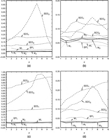
Size of testing conditional mean at 5% level—(a) DGP A.0: AR(1)–N(0,1), (b) DGP A.0: AR(1)–exponential, (c) DGP A.0: AR(1)–mixed normal, (d) DGP A.0: AR(1)–t5.
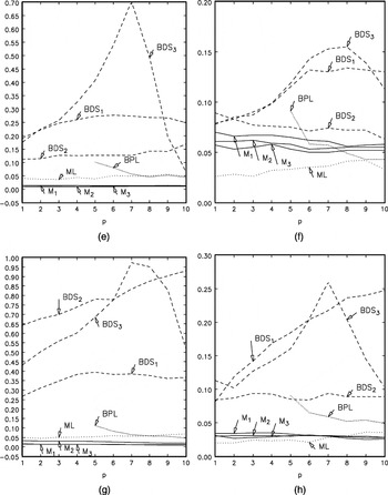
Size of testing conditional mean at 5% level—(e) DGP C.0: AR(4)–N(0,1), (f) DGP C.0: AR(4)–exponential, (g) DGP C.0: AR(4)–mixed normal, (h) DGP C.0: AR(4)–t5.
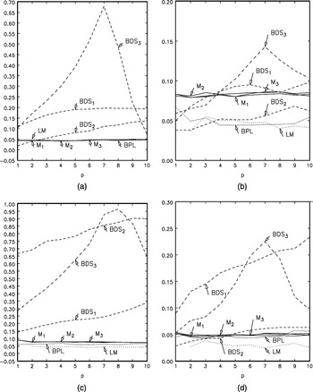
Size of testing conditional variance at 5% level—(a) DGP B.0: ARCH(1)–N(0,1), (b) DGP B.0: ARCH(1)–exponential, (c) DGP B.0: ARCH(1)–mixed normal, (d) DGP B.0: ARCH(1)–t5.
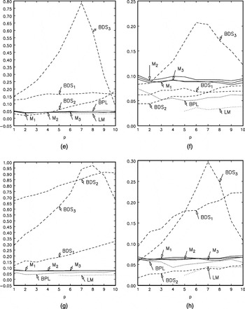
Size of testing conditional variance at 5% level—(e) DGP D.0: ARCH(4)–N(0,1), (f) DGP D.0: ARCH(4)–exponential, (g) DGP D.0: ARCH(4)–mixed normal, (h) DGP D.0: ARCH(4)–t5.
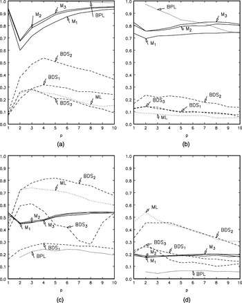
Size-corrected power of testing conditional mean at 5% level—(a) DGP A.1: AR(2)–N(0,1), (b) DGP A.2: ARMA(1,1)–N(0,1), (c) DGP A.3: bilinear–N(0,1), (d) DGP A.4: nonlinear MA–N(0,1).
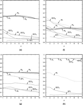
Size-corrected power of testing conditional mean at 5% level—(e) DGP A.5: TAR–N(0,1), (f) DGP A.6: Markov switching–N(0,1), (g) DGP A.7: SIGN–N(0,1), (h) DGP A.8: tent map.
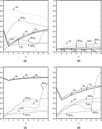
Size-corrected power of testing conditional variance at 5% level—(a) DGP B.1: ARCH(2)–N(0,1), (b) DGP B.2: GARCH(1,1)–N(0,1), (c) DGP B.3: EGARCH–N(0,1), (d) DGP B.4: stochastic volatility–N(0,1).
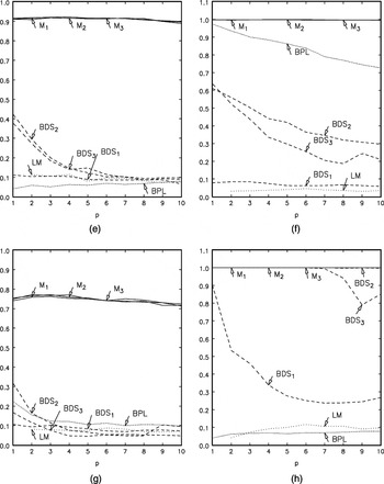
Size-corrected power of testing conditional variance at 5% level—(e) DGP B.5: bilinear–N(0,1), (f) DGP B.6: TAR–N(0,1), (g) DGP B.7: nonlinear MA–N(0,1), (h) DGP B.8: logistic map.
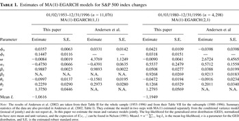
Estimates of MA(1)-EGARCH models for S&P 500 index changes
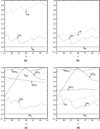
Empirical application—(a) Asymptotic p-values: 1953–1996, (b) bootstrap p-values: 1953–1996, (c) asymptotic p-values: 1980–1996, (d) bootstrap p-values: 1980–1996.
 You have
Access
- 67
- Cited by