1 Introduction
Viscoelastic liquid exhibits singular nonlinear behaviour and there are quite a few unique outcomes of high elasticity verified in experiments (e.g. Boger & Walters Reference Boger and Walters1993). Extrudate swelling, for example, expresses complicated relaxation of the elastic stress accumulated in Poiseuille flow often combined with extensional deformation inside a channel. As the flow intensity further increases, the fluid often displays elastic instabilities such as symmetry breaking or spatio-temporal fluctuation of the flow field (e.g. Afonso et al. Reference Afonso, Oliveira, Pinho and Alves2011; Kwon Reference Kwon2014). Such unstable phenomena manifested by the extrudate are termed the sharkskin and melt fractures (Tordella Reference Tordella1956; Leonov & Prokunin Reference Leonov and Prokunin1994; Denn Reference Denn2001).
Notable distortion of the extrudate out from the Poiseuille flow has been observed and was first reported by Garvey, Whitlock & Freese (Reference Garvey, Whitlock and Freese1942), with Tordella (Reference Tordella1956) naming such behaviour as a melt fracture. This interfacial instability is sometimes accompanied by a longitudinal scratch of extrudate at the onset of melt fracture (Piau, Kissi & Tremblay Reference Piau, Kissi and Tremblay1990; Kissi, Piau & Toussaint Reference Kissi, Piau and Toussaint1997; Piau, Nigen & Kissi Reference Piau, Nigen and Kissi2000), but the instability is usually displayed in distinctive forms, of which the most representative are the sharkskin and gross melt fracture often with a periodic pattern (Boger & Walters Reference Boger and Walters1993). On most occasions, the extrudate instability is observed in extrusion from a capillary die, and equivalent phenomena for film blowing (Ramamurthy Reference Ramamurthy1986) and for planar die extrusion (Kissi & Piau Reference Kissi and Piau1994) have also been investigated, where the effect of the die wall character on the melt fracture has been extensively examined. Although verification of its origin and cause seems far from complete resolution, one can find excellent reviews on this long-standing problem. Larson (Reference Larson1992) and Shaqfeh (Reference Shaqfeh1996) have compiled various phenomena of viscoelastic instability in general, and quite a detailed summary of research results on melt fracture including theoretical considerations can be found (Leonov & Prokunin Reference Leonov and Prokunin1994; Graham Reference Graham1999; Denn Reference Denn2001). The book by Koopmans, Doelder & Molenaar (Reference Koopmans, Doelder and Molenaar2010) also presents collections of photos, theoretical modelling and simulations.
Streamlines of finite curvature combined with high tensile stress are proven to control the onset of asymptotic instability of viscoelastic flow (Pakdel & McKinley Reference Pakdel and McKinley1996), and thus the creeping flow along the straight channel is always linearly stable. On the other hand, nonlinear subcritical transition to an unstable regime under finite disturbance also exists in this type of flow (Meulenbroek et al. Reference Meulenbroek, Storm, Bertola, Wagner, Bonn and van Saarloos2003; Pan et al. Reference Pan, Morozov, Wagner and Arratia2013). In the common flow situation resulting in the melt fracture, streamlines are not straight any more, since their curvature becomes non-vanishing at least near the die exit due to swelling as well as the abrupt conversion of the Poiseuille flow with no-slip on the wall to a free surface flow. Therefore, the occurrence of nonlinear dynamic instability via flow bifurcation caused by high elasticity along the curved streamlines is highly probable even with no wall slip. In this paper, employing a straightforward computation scheme of a finite element method for the mathematically stable Leonov constitutive equation, we try to clarify the cause of melt fracture in terms of two-dimensional (2-D) flow dynamic factors without taking slip effects into account.
There appears to exist a variety of causes that result in melt fracture. Whereas dissipative heat, melt compressibility, supercritical or subcritical transition or even mechanical failure of the liquid itself have been proposed to be the origin of the extrudate instability, the die wall slip is considered to be the most important mechanism leading to melt fracture (Leonov & Prokunin Reference Leonov and Prokunin1994; Graham Reference Graham1999; Denn Reference Denn2001). Wall slip of an elastic liquid alone is not a simple problem at all, and whether it results from stretching and uncoiling (Brochard & de Gennes Reference Brochard and de Gennes1992; Ajdari et al. Reference Ajdari, Brohard-Wyart, de Gennes, Leibler, Viovy and Rubinstein1994) or adsorption and desorption (Inn & Wang Reference Inn and Wang1996) of chains attached to the wall is not yet certain. As a matter of course, there have been many in-depth discussions regarding the unambiguous proof of wall slip (Migler, Hervet & Leger Reference Migler, Hervet and Leger1993; Migler et al. Reference Migler, Massey, Hervet and Leger1994) and whether the slip plays a central role in melt fracture and sharkskin dynamics (for example cf. Kissi & Piau Reference Kissi and Piau1994). As a result, many attempts to delineate the melt fracture in terms of wall slip models have been made based on various physical assumptions. Adewale & Leonov (Reference Adewale and Leonov1997) have described melt fracture, introducing the concept of solid-like transition of the viscoelastic liquid on the channel wall under high elastic stress. A phenomenological model of slip induced by transition of the density parameter of entanglements between bulk chains and chains attached on the wall has also been proposed (Black & Graham Reference Black and Graham1996). Shore et al. (Reference Shore, Ronis, Piché and Grant1997) have explained the wall slip in terms of the first order phase transition expressed by the Ginzburg–Landau free energy functional. Employing the ‘slip equation’ for the die wall, Brasseur et al. (Reference Brasseur, Fyrillas, Georgiou and Crochet1998) have straightforwardly demonstrated periodic oscillation of an axisymmetric extrudate surface.
Notwithstanding scientific interest and practical importance in understanding these purely elastic instabilities, a theoretical description of melt fracture has been a formidable task to achieve in the field of computational viscoelastic fluid dynamics. Even though the slip on the channel wall may be essential for accurate expression of a melt fracture, the flow simulation herein presents a direct attempt to verify its additional possible origin in the case of flow without wall slip or the other factors mentioned above. In other words, this work only considers extrudate surface undulation caused purely by the flow dynamic fluctuation. As mentioned above, periodic oscillation of an axisymmetric extrudate surface has been modelled by Brasseur et al. (Reference Brasseur, Fyrillas, Georgiou and Crochet1998) with a finite element approximation implemented. On the other hand, due to the difficulty in the computational modelling of highly elastic flow problems, straightforward computational verification of the viscoelastic melt fracture in a 2-D (or axisymmetric) or 3-D flow domain is very rare. However, recent progress in the computational modelling of viscoelastic flows has substantially increased our understanding and enabled a plausible description of several elastic flow instabilities. Especially the introduction of a matrix–logarithmic formulation for the viscoelastic constitutive models (Fattal & Kupferman Reference Fattal and Kupferman2004) has constituted a crucial breakthrough in the modelling of elastic flow instability. Numerical simulations of elastic flow asymmetry in a symmetric domain (Poole, Alves & Oliveira Reference Poole, Alves and Oliveira2007), vortex fluctuation through a contraction channel (Afonso et al. Reference Afonso, Oliveira, Pinho and Alves2011; Kwon Reference Kwon2014), periodic 3-D pattern behind a cylinder (Sahin Reference Sahin2013) and melt fracture of extrudate from Poiseuille flow in the contraction die (Kwon Reference Kwon2015) are the results obtained under this matrix-log transformation.
The melt fracture caused by elastic flow instability in the limit of a vanishing inertial effect is essentially different from the surface distortion due to the turbulence in a viscous flow driven by the inertial force and its satisfactory comprehension is still beyond reach. Its control is also important in practice since manufacturing speed in the process of polymeric and other complex fluids is mainly bounded by the occurrence of such instabilities. While especially the wall slip effect is considered as the main cause giving rise to this instability (Adewale & Leonov Reference Adewale and Leonov1997; Graham Reference Graham1999; Denn Reference Denn2001), in this paper, an additional possible origin of melt fracture under a strict no slip condition on the liquid/solid interface is investigated. In the previous work (Kwon Reference Kwon2015), computational modelling of melt fracture for the extrudate released from a planar contraction channel has been performed, but clear reasoning for the dynamic mechanism is still lacking. In the current study, we simplify the problem of the melt fracture by considering the flow inside a straight planar channel or die, and then pursue the goal of confirming a supplementary possible origin of instability especially related to the onset of sharkskin. At least one of the transitions undergone in the viscoelastic flow dynamics is verified as the subcritical bifurcation to periodic instability seemingly associated with high elastic stress along die exit streamlines of finite curvature and the resultant small vortices near the die lip. Thus, this work is presumably considered a far from a complete analysis of melt fracture which should inevitably incorporate the slip phenomena in the modelling, rather it offers a robust framework for directly analysing its fluid mechanical mechanism without further introduction of a speculative hypothesis. In other words, if one implements an algorithm of wall stick and slip (e.g. Black & Graham Reference Black and Graham1996; Adewale & Leonov Reference Adewale and Leonov1997) to this framework of modelling, a complete analysis of unstable extrudate profile seems attainable.
This paper is organized as follows. The equations and numerical method are described in § 2, and the results of the computation and a possible cure for melt fracture are discussed in § 3. Then we provide concluding remarks in § 4.
2 Equations and numerical scheme
Assigning a vanishing Reynolds number
 $(Re\equiv \unicode[STIX]{x1D70C}UH/\unicode[STIX]{x1D702}=0)$
that supposes the flow to have a negligible inertial force relative to the viscous one, we focus on the melt fracture caused solely by liquid elasticity at high Deborah number
 $(De\equiv \unicode[STIX]{x1D703}U/H\gg 1)$
, which implies a considerable degree of elasticity accumulated during the flow. Here
 $U$
and
 $H$
are the characteristic velocity (mean axial speed in the channel) and length, respectively,
 $\unicode[STIX]{x1D70C}$
is the density,
 $\unicode[STIX]{x1D702}$
is the viscosity and
 $\unicode[STIX]{x1D703}$
is the relaxation time of the incompressible liquid. In order to assess the liquid elasticity in the set of equations, the Leonov model (Leonov Reference Leonov1976) is implemented into the momentum and the continuity equations
 $$\begin{eqnarray}-\unicode[STIX]{x1D735}p+\unicode[STIX]{x1D735}\boldsymbol{\cdot }\unicode[STIX]{x1D749}=\mathbf{0},\quad \unicode[STIX]{x1D735}\boldsymbol{\cdot }\boldsymbol{v}=0.\end{eqnarray}$$
Here
 $p$
is the pressure,
 $\unicode[STIX]{x1D749}$
is the extra stress tensor and
 $\boldsymbol{v}$
is the velocity vector. The Leonov model is one of a few constitutive equations which are mathematically well posed (Kwon & Leonov Reference Kwon and Leonov1995), it gives a pertinent material description (Simhambhatla & Leonov Reference Simhambhatla and Leonov1995) and is composed of the evolution equation and the stress relation
 $$\begin{eqnarray}\unicode[STIX]{x1D658}_{(1)}+2\unicode[STIX]{x1D658}\boldsymbol{\cdot }e_{p}=\mathbf{0},\end{eqnarray}$$
 $$\begin{eqnarray}\unicode[STIX]{x1D658}_{(1)}=\frac{\unicode[STIX]{x2202}\unicode[STIX]{x1D658}}{\unicode[STIX]{x2202}t}+\boldsymbol{v}\boldsymbol{\cdot }\unicode[STIX]{x1D735}\unicode[STIX]{x1D658}-\unicode[STIX]{x1D735}\boldsymbol{v}^{\text{T}}\boldsymbol{\cdot }\unicode[STIX]{x1D658}-\unicode[STIX]{x1D658}\boldsymbol{\cdot }\unicode[STIX]{x1D735}\boldsymbol{v},\quad e_{p}=\frac{1}{4\unicode[STIX]{x1D703}}\left[\left(\unicode[STIX]{x1D658}-\frac{I_{1}}{3}\unicode[STIX]{x1D739}\right)-\left(\unicode[STIX]{x1D658}^{-1}-\frac{I_{2}}{3}\unicode[STIX]{x1D739}\right)\right],\end{eqnarray}$$
 $$\begin{eqnarray}\unicode[STIX]{x1D749}=2\unicode[STIX]{x1D658}\boldsymbol{\cdot }\frac{\unicode[STIX]{x2202}\unicode[STIX]{x1D6F7}}{\unicode[STIX]{x2202}\unicode[STIX]{x1D658}}+2\unicode[STIX]{x1D702}se=(1-s)G\left(\frac{I_{1}}{3}\right)^{n}\unicode[STIX]{x1D658}+2\unicode[STIX]{x1D702}se,\end{eqnarray}$$
 $$\begin{eqnarray}D=\text{tr}\left(2\unicode[STIX]{x1D658}\boldsymbol{\cdot }\frac{\unicode[STIX]{x2202}\unicode[STIX]{x1D6F7}}{\unicode[STIX]{x2202}\unicode[STIX]{x1D658}}\boldsymbol{\cdot }e_{p}\right),\quad \unicode[STIX]{x1D6F7}=\frac{3}{2}\frac{(1-s)G}{n+1}\left[\left(\frac{I_{1}}{3}\right)^{n+1}-1\right],\end{eqnarray}$$
where dimensionless
 $\unicode[STIX]{x1D658}$
is the elastic Finger strain tensor,
 $\unicode[STIX]{x1D658}_{(1)}$
is its upper convected time derivative,
 $I_{1}$
and
 $I_{2}$
are the first and second invariants of
 $\unicode[STIX]{x1D658}$
, respectively,
 $e=(\unicode[STIX]{x1D735}\boldsymbol{v}+\unicode[STIX]{x1D735}\boldsymbol{v}^{\text{T}})/2$
is the strain rate,
 $\unicode[STIX]{x1D739}$
is the unit tensor and
 $\text{tr}$
is the trace operator acting on the second rank tensor. The linear viscoelastic parameters
 $G$
and
 $s$
are elastic modulus and dimensionless solvent viscosity ratio, respectively, and thus
 $\unicode[STIX]{x1D702}=G\unicode[STIX]{x1D703}$
corresponds to the total zero-shear viscosity while
 $s\unicode[STIX]{x1D702}$
is the solvent viscosity. There also exists a nonlinear parameter
 $n$
, the admissible range of which for mathematical stability is
 $n>0$
(Kwon & Leonov Reference Kwon and Leonov1995). It controls the degree of nonlinear viscoelastic behaviour, that is, larger
 $n$
leads to weaker shear thinning but stronger extension hardening at the same time. Equations (2.5) display the association of the constitutive relation with the thermodynamics, where
 $D$
and
 $\unicode[STIX]{x1D6F7}$
are mechanical dissipation and elastic potential, respectively.
The rheological field equations (2.2)–(2.3) are rewritten into the matrix–logarithmic formulation in terms of
 $\unicode[STIX]{x1D65D}=\log \unicode[STIX]{x1D658}$
suggested by Fattal & Kupferman (Reference Fattal and Kupferman2004), and the resultant form is as follows.
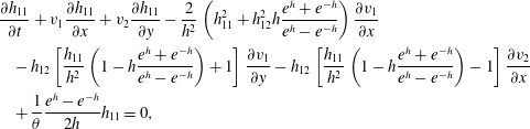 $$\begin{eqnarray}\displaystyle & & \displaystyle \frac{\unicode[STIX]{x2202}h_{11}}{\unicode[STIX]{x2202}t}+v_{1}\frac{\unicode[STIX]{x2202}h_{11}}{\unicode[STIX]{x2202}x}+v_{2}\frac{\unicode[STIX]{x2202}h_{11}}{\unicode[STIX]{x2202}y}-\frac{2}{h^{2}}\left(h_{11}^{2}+h_{12}^{2}h\frac{e^{h}+e^{-h}}{e^{h}-e^{-h}}\right)\frac{\unicode[STIX]{x2202}v_{1}}{\unicode[STIX]{x2202}x}\nonumber\\ \displaystyle & & \displaystyle \quad -\,h_{12}\left[\frac{h_{11}}{h^{2}}\left(1-h\frac{e^{h}+e^{-h}}{e^{h}-e^{-h}}\right)+1\right]\frac{\unicode[STIX]{x2202}v_{1}}{\unicode[STIX]{x2202}y}-h_{12}\left[\frac{h_{11}}{h^{2}}\left(1-h\frac{e^{h}+e^{-h}}{e^{h}-e^{-h}}\right)-1\right]\frac{\unicode[STIX]{x2202}v_{2}}{\unicode[STIX]{x2202}x}\nonumber\\ \displaystyle & & \displaystyle \quad +\,\frac{1}{\unicode[STIX]{x1D703}}\frac{e^{h}-e^{-h}}{2h}h_{11}=0,\end{eqnarray}$$
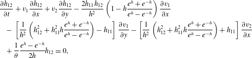 $$\begin{eqnarray}\displaystyle & & \displaystyle \frac{\unicode[STIX]{x2202}h_{12}}{\unicode[STIX]{x2202}t}+v_{1}\frac{\unicode[STIX]{x2202}h_{12}}{\unicode[STIX]{x2202}x}+v_{2}\frac{\unicode[STIX]{x2202}h_{12}}{\unicode[STIX]{x2202}y}-\frac{2h_{11}h_{12}}{h^{2}}\left(1-h\frac{e^{h}+e^{-h}}{e^{h}-e^{-h}}\right)\frac{\unicode[STIX]{x2202}v_{1}}{\unicode[STIX]{x2202}x}\nonumber\\ \displaystyle & & \displaystyle \quad -\,\left[\frac{1}{h^{2}}\left(h_{12}^{2}+h_{11}^{2}h\frac{e^{h}+e^{-h}}{e^{h}-e^{-h}}\right)-h_{11}\right]\frac{\unicode[STIX]{x2202}v_{1}}{\unicode[STIX]{x2202}y}-\left[\frac{1}{h^{2}}\left(h_{12}^{2}+h_{11}^{2}h\frac{e^{h}+e^{-h}}{e^{h}-e^{-h}}\right)+h_{11}\right]\frac{\unicode[STIX]{x2202}v_{2}}{\unicode[STIX]{x2202}x}\nonumber\\ \displaystyle & & \displaystyle \quad +\,\frac{1}{\unicode[STIX]{x1D703}}\frac{e^{h}-e^{-h}}{2h}h_{12}=0,\end{eqnarray}$$
where
 $h=\sqrt{h_{11}^{2}+h_{12}^{2}}$
is the eigenvalue of the
 $\unicode[STIX]{x1D65D}$
tensor in two dimensions. The incompressibility of the liquid exerts the condition
 $\det \unicode[STIX]{x1D658}=1$
in the case of the Leonov model and for
 $\unicode[STIX]{x1D65D}$
it becomes
 $\text{tr}\,\unicode[STIX]{x1D65D}=0$
, and thus the second eigenvalue and
 $h_{22}$
of
 $\unicode[STIX]{x1D65D}$
are
 $-h$
and
 $-h_{11}$
, respectively. In fact,
 $\unicode[STIX]{x1D658}$
and
 $\unicode[STIX]{x1D65D}$
imply recoverable Finger and Hencky strain tensors. This revision of the equations offers immediate advantage in numerical approximations, since it automatically preserves the positive definiteness of
 $\unicode[STIX]{x1D658}$
and bestows improved interpolation (Kwon Reference Kwon2014, Reference Kwon2015).
A finite element method is applied to solve the above set of equations and a fully implicit time integration of the second or third order is used. A straightforward mixed method (cubic for
 $\boldsymbol{v}$
and quadratic interpolation for
 $p$
and
 $\unicode[STIX]{x1D65D}$
) is employed without streamline upwinding and elastic–viscous stress splitting (EVSS or its variants) modification (e.g. Baaijens Reference Baaijens1998; Owens & Phillips Reference Owens and Phillips2002). The SUPG (streamline upwind/Petrov–Galerkin) and DEVSS (discrete EVSS) methods are proven to introduce a significant degree of numerical diffusion that is highly dependent on the value of algorithm-specific parameters and sometimes even spoils the computational stability (Kwon Reference Kwon2014, Reference Kwon2015). This result regarding such an unfavourable effect of the numerical techniques will surely rely on and vary with the type of evolution equations used, especially in highly elastic flow modelling, and therefore extreme care has to be taken when one adopts a particular approximation scheme especially in the case of introducing numerical diffusion. The computational scheme mentioned above is integrated into the software COMSOL Multiphysics, in which the level set method is the main facility to approximately delineate the surface of the extrudate. Even though numerical dissipation introduced by the level set expression for the extrudate surface becomes inevitable chiefly due to its rather thick representation of the interface, a mesh convergence test has confirmed the qualitative and quantitative accuracy of the solutions. A small value for the interfacial tension (scaled by
 $GH$
) between elastic liquid and low viscous fluid is set, at 0.001. The detail of the viscoelastic constitutive equation and numerical algorithm may be found in the previous works by Kwon (Reference Kwon2014, Reference Kwon2015).
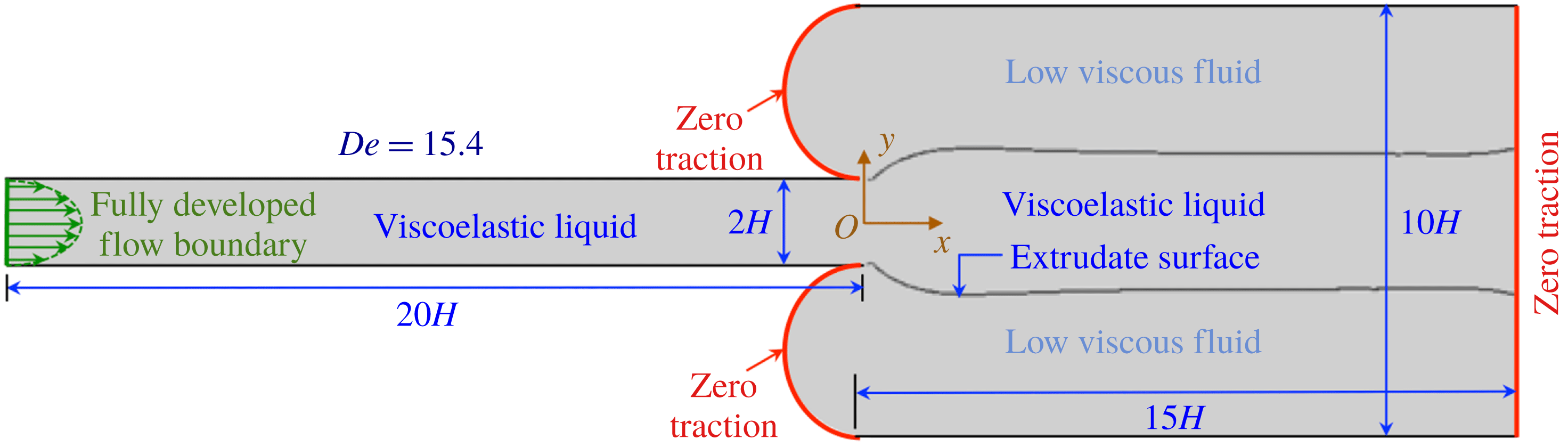
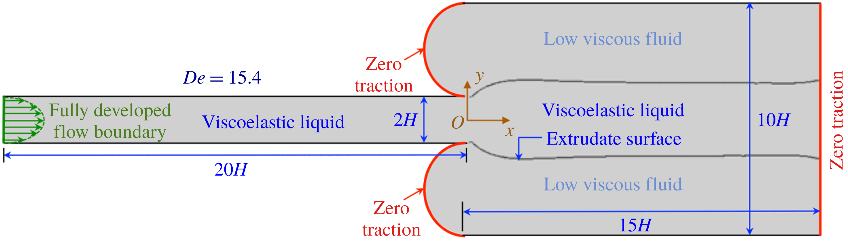
Figure 1 illustrates the problem domain considered in this study, which is primarily composed of two regions corresponding to the flows inside and outside of the narrow channel. The values of
 $2H$
and
 $20H$
are assigned as the height and length of this planar die, respectively. The dimensionless coordinates
 $x$
and
 $y$
are defined in terms of
 $H$
as the unit measure, where the origin is located at the centre of the channel exit. The pressure
 $p$
and stress
 $\unicode[STIX]{x1D749}$
are scaled with
 $G$
and the dimensionless time
 $t$
with
 $\unicode[STIX]{x1D703}$
. At the entrance, fully developed steady velocity and stress profiles are appointed as boundary conditions. The initial condition in the narrow channel is specified with fully developed flow values, while the flow of low viscous fluid outside the die starts from the stationary stress-free state
 $(t<0)$
, and thus the initial interface between elastic and viscous fluids is vertically located at the die exit. In this setting at the moment the flow starts, the narrow die is filled with viscoelastic liquid, while outside the die viscous fluid occupies the wide channel. Even though the initial state of the flow is not in the complete rest state, we term this flow simulation as the computation of the start-up flow from rest in order to distinguish it from the hysteretic flow test explained later. Viscosity of the surrounding low viscosity fluid is equal to
 $\unicode[STIX]{x1D702}/1000$
, that is, the zero-shear viscosity of the elastic liquid is 1000 times higher than that of the surrounding fluid. Both elastic and viscous fluids are assigned zero density and thus in the whole computational domain the flow is assumed inertialess. The condition of zero traction is imposed on 2 half-circular boundaries as well as at the outlet (boundaries in red curves), and all of the horizontal boundaries are assigned as no slip. Therefore, we do not allow any possibility of a melt fracture caused by the slip on the channel wall but focus only on instability due to fluid dynamics involving flow elasticity. The half-circular shape for viscous flow inlet is applied in order to minimize the effect of the traction-free boundary on the viscoelastic flow and also to remove the probability of losing elastic liquid via it flowing outside of the boundary in the extreme case of instability. For all the calculations, the solvent viscosity ratio
 $s$
and the nonlinear parameter
 $n$
are fixed as 0.005 and 1, respectively, with which the liquid seems to plausibly simulate the extrudate instability exemplified in the previous work (Kwon Reference Kwon2015).
Schematic of flow geometry. The profile of extrudate swelling described in a steady flow of
 $De=15.4$
.
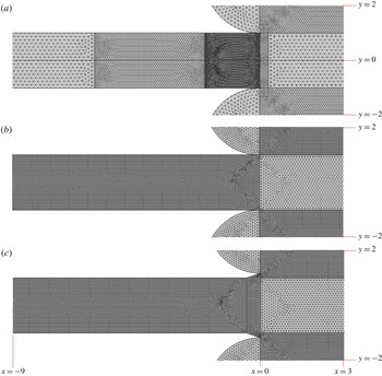
Partial view of the structure of the mesh applied for the spatial discretization of the problem domain (the region of
 $-9<x<3$
and
 $-2<y<2$
) is shown in figure 2(a), which is composed of triangular elements. It is the main mesh in this study, designed to be perfectly symmetric along the horizontal centreline (the line of
 $y=0$
) in order to prevent fallacious flow asymmetry due to spatial discretization artefacts. On the other hand, for examination of the effect of die geometry, we intentionally employ a mesh that is not symmetric along the centreline (figure 2
b) and investigate whether the modification of die exit shown in figure 2(c) is capable of recovering flow field symmetry even under asymmetric spatial discretization.
(a) Partial view of symmetric main mesh employed in the study of flow instability. (b) Mesh (asymmetric) employed in the study of the effect of exit modification. (c) One example mesh (asymmetric) for the flow geometry with exit modification (slope 0.34).
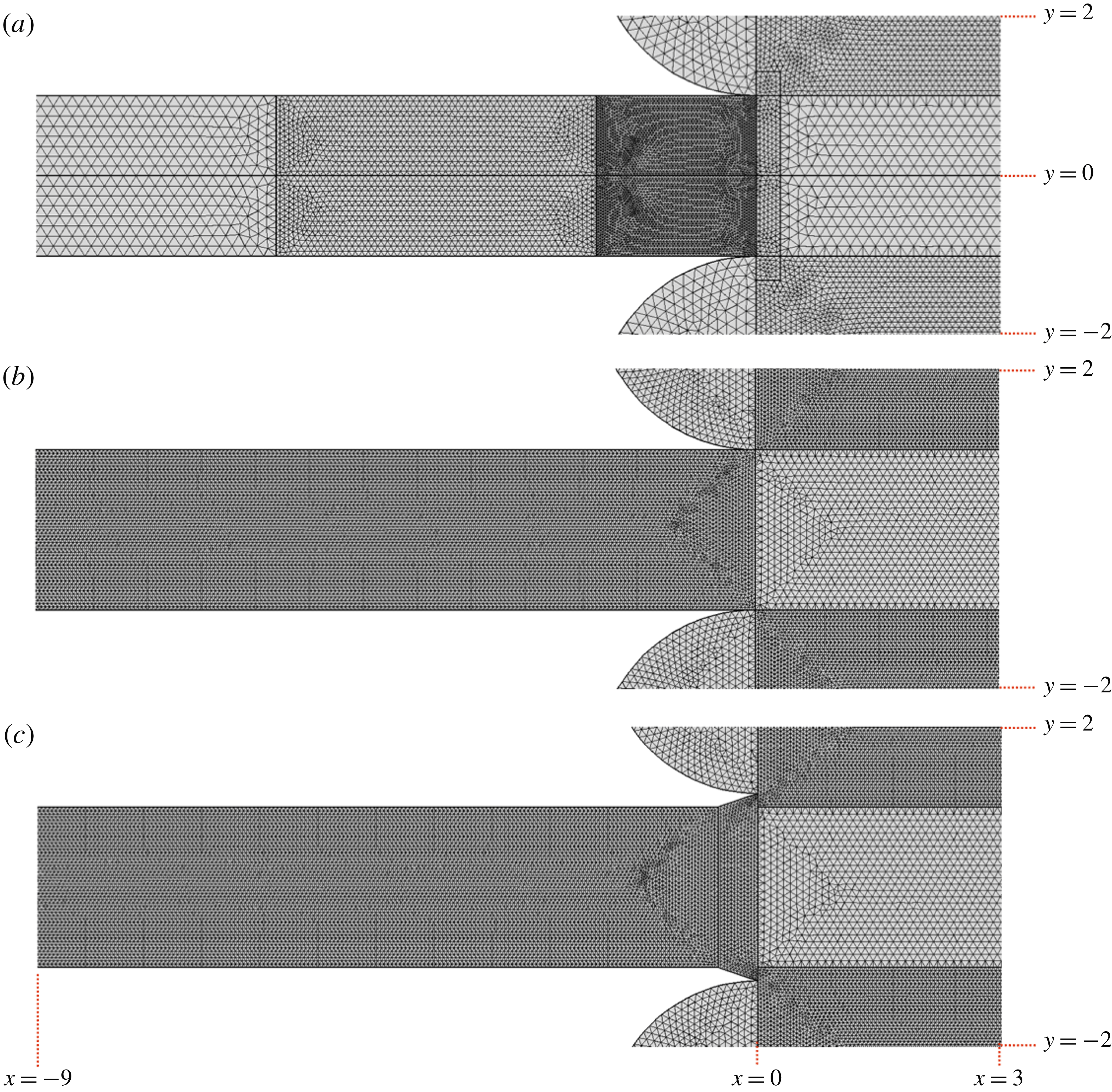
In order to verify convergence and accuracy according to spatial refinement, 4 different meshes, including two coarser and one finer ones, have been tested for the main symmetric discretization of figure 2(a). In brief, all the meshes yield almost identical solutions, at least for the current parameters, when the flow attains steady state. In the case of weak elastic instability, later termed the sharkskin fracture, with temporal fluctuation, equivalent solutions have been obtained for the mesh of figure 2(a) and for the finer one. However, when the computed flow exhibits strong instability designated as gross melt fracture, the test for the finest refinement could not be completed as the computation becomes too demanding and for other meshes sufficient accuracy was not guaranteed. Therefore, in this case, numerical solutions corresponding to the chaotic flow of strong instability have to be considered correct in a qualitative sense. For the problem of investigating the effect of die geometry on the instability, only one set of meshes such as those of figure 2(b,c) and corresponding ones with different diverging wall slopes have been employed, and the solution again possesses only qualitative meaning and approximate potency.
One illustration of the extrudate profile apparently in the steady state at
 $De=15.4$
is also drawn in figure 1, and it expresses a typical extrudate swelling following the Poiseuille flow in the channel. Due to the imposed zero traction on the boundaries outside of the die (2 half-circular and 1 vertical boundary in red), the flow of surrounding low viscosity fluid simply results from the drag of the extrudate.
3 Results and discussion
3.1 Bifurcations and chaotic transition to melt fracture
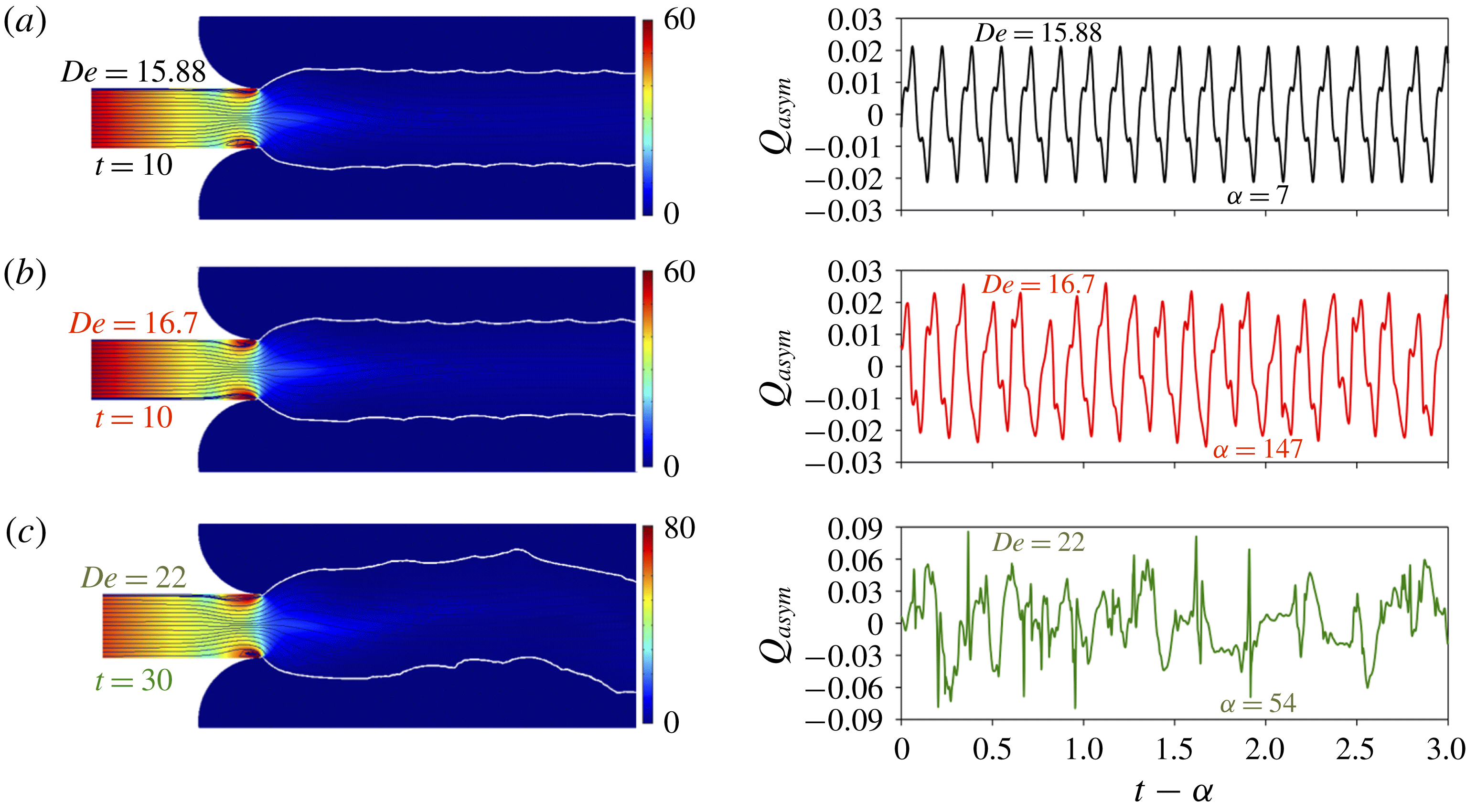
For three different values of
 $De$
, figure 3 discloses representative extrudate profiles including streamlines and pressure contours at fixed instants (left) and the time variation of
 $Q_{asym}$
, the degree of flow rate asymmetry (right). In order to probe the degree of elastically driven flow asymmetry,
 $Q_{asym}\equiv (Q_{up}-Q_{low})/(Q_{up}+Q_{low})$
is defined, in which
 $Q_{up}$
and
 $Q_{low}$
are flow rates through the upper and lower halves of the channel exit, respectively. Only the mesh that is perfectly symmetric about the
 $x$
-axis is used (figure 2
a), hence the instability manifested in the form of symmetry breaking of solutions is not at all associated with any artefact of the spatial discretization.
Streamlines and extrudate surfaces on the contour of pressure at time instants indicated (left) and the degree of flow rate asymmetry
 $Q_{asym}$
for
 $\unicode[STIX]{x1D6FC}<t<\unicode[STIX]{x1D6FC}+3$
(right): (a)
 $De=15.88$
, (b)
 $De=16.7$
, (c)
 $De=22$
.
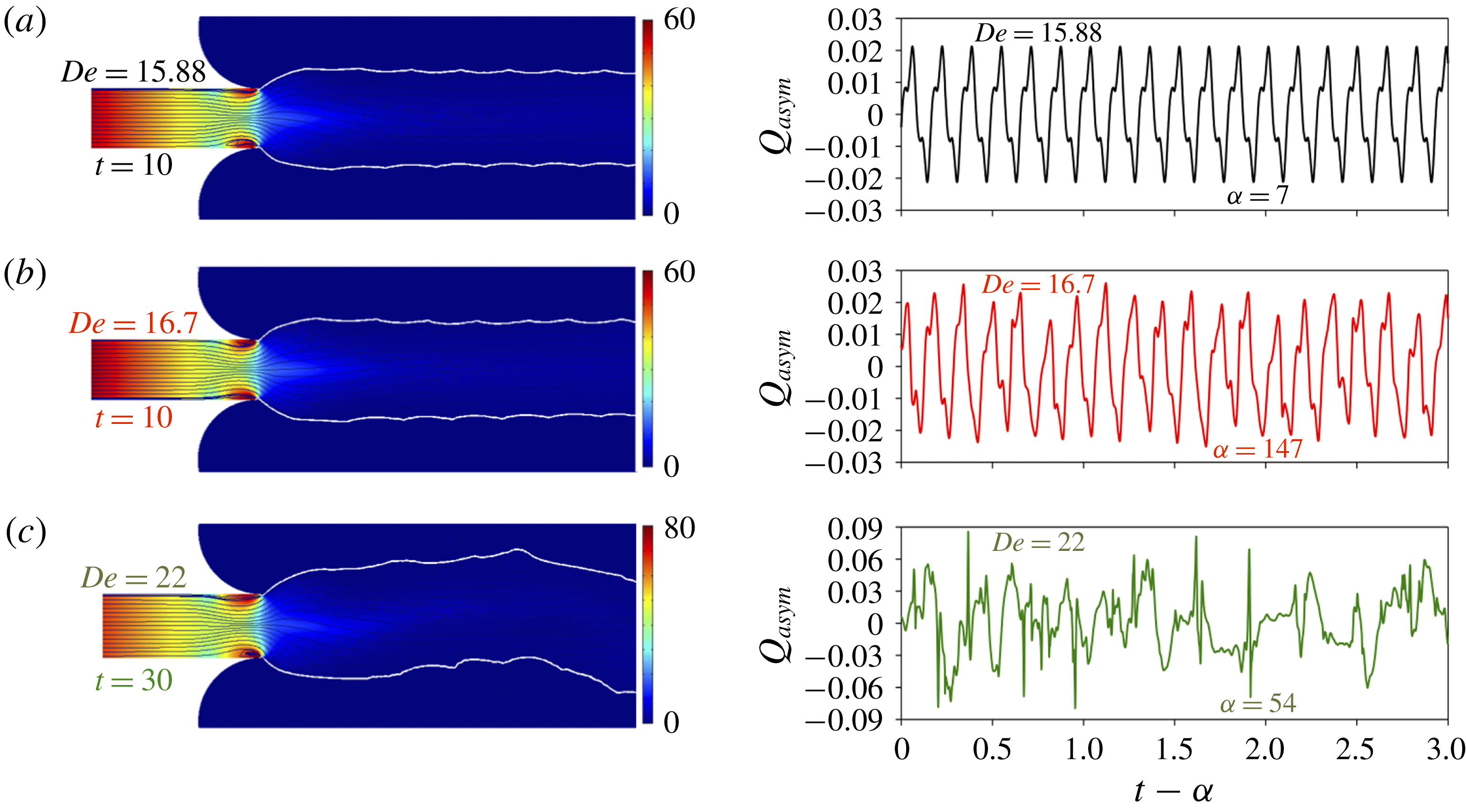
Since every solution in figure 3 conforms to the elastically unstable regime, the flows never attain steady state and exhibit conspicuous fluctuations that certify the unstable flow dynamics after the subcritical bifurcation from the steady state with increasing
 $De$
. Whereas the extrudate profiles for
 $De=15.88$
and 16.7 (figure 3
a,b left) depict a more or less regular structure of the melt fracture, presumably indicative of sharkskin, at higher
 $De=22$
(figure 3
c left) gross melt fracture appears (the simulated animation can be found in the supplementary movies available at https://doi.org/10.1017/jfm.2018.659). Creeping elastic flow in the straight channel and therefore with straight streamlines is known to be linearly stable, however, the singular points located at the die lip induce a high pressure gradient (and also high stress due to the molecular stretching caused by the abrupt change of boundary conditions from the no-slip wall to free interface) as well as finite streamline curvature, which is explicitly demonstrated near the exit wall on the left of figure 3. Even recurring tiny vortices (alternating with a short lifetime) are existent and can be observed near singularities. The high stress near these tips at the channel exit is thought to regulate the onset of instability that corresponds to the subcritical transition. On the right of figure 3 the symmetry breaking of the flow field due to elastic instability is more quantitatively expressed in terms of
 $Q_{asym}$
in the time interval
 $\unicode[STIX]{x1D6FC}<t<\unicode[STIX]{x1D6FC}+3$
(for instance in the case of symmetric flow
 $Q_{asym}=0$
). According to the temporal behaviour of this parameter, the solution corresponds to three such distinct flow regimes as a periodic state or limit cycle at
 $De=15.88$
(figure 3
a), a quasiperiodic state at 16.7 (figure 3
b) and an aperiodic state at 22 (figure 3
c).
The periodic limit cycle of figure 3(a) indeed emanates from the second steady state via the subcritical bifurcation. In the lower
 $De$
, another weak periodic fluctuation exists followed by this second steady flow with increasing
 $De$
, and it is discussed in more detail with figures 4 and 5. In real viscoelastic flow and in regard to figure 3(c), such aperiodic chaotic flow seems to mainly originate from the high extensional stress incurred in the contraction flow or by strong wall slip (or via subcritical dynamic transition inside the channel described in Meulenbroek et al.
Reference Meulenbroek, Storm, Bertola, Wagner, Bonn and van Saarloos2003), and thus a developed elastic instability or wall slip may regulate the melt fracture outside the die. Nevertheless, in this study, possible gross melt fracture modelled simply by chaotic dynamic transition (due to singularity at the die lip) is naïvely demonstrated, however low its practical probability might be. For rigorous analysis of elastic flow instability including melt fracture, every possible origin of instability, including the current chaotic regime, has to be considered altogether in formulating and modelling the problem.
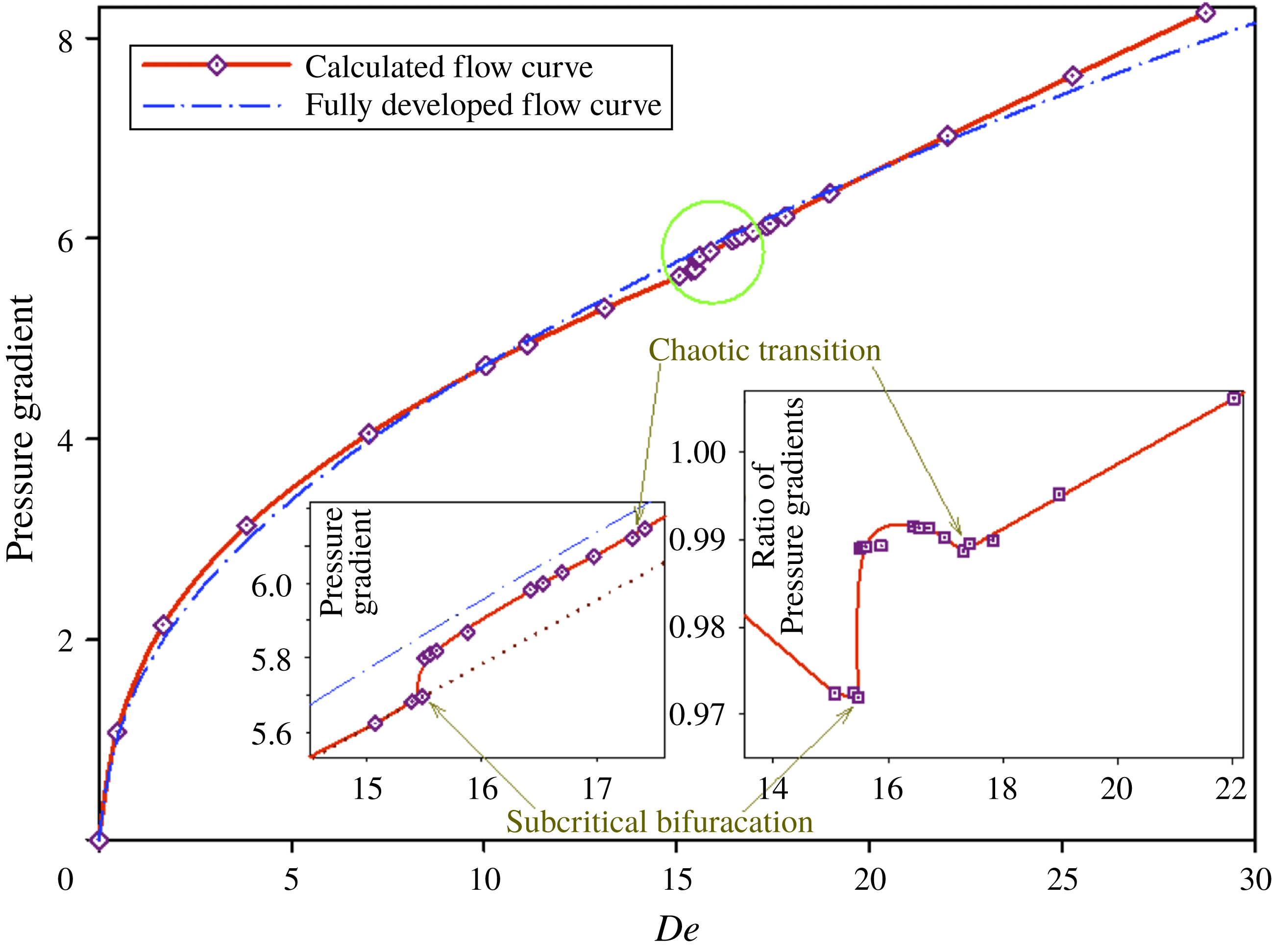
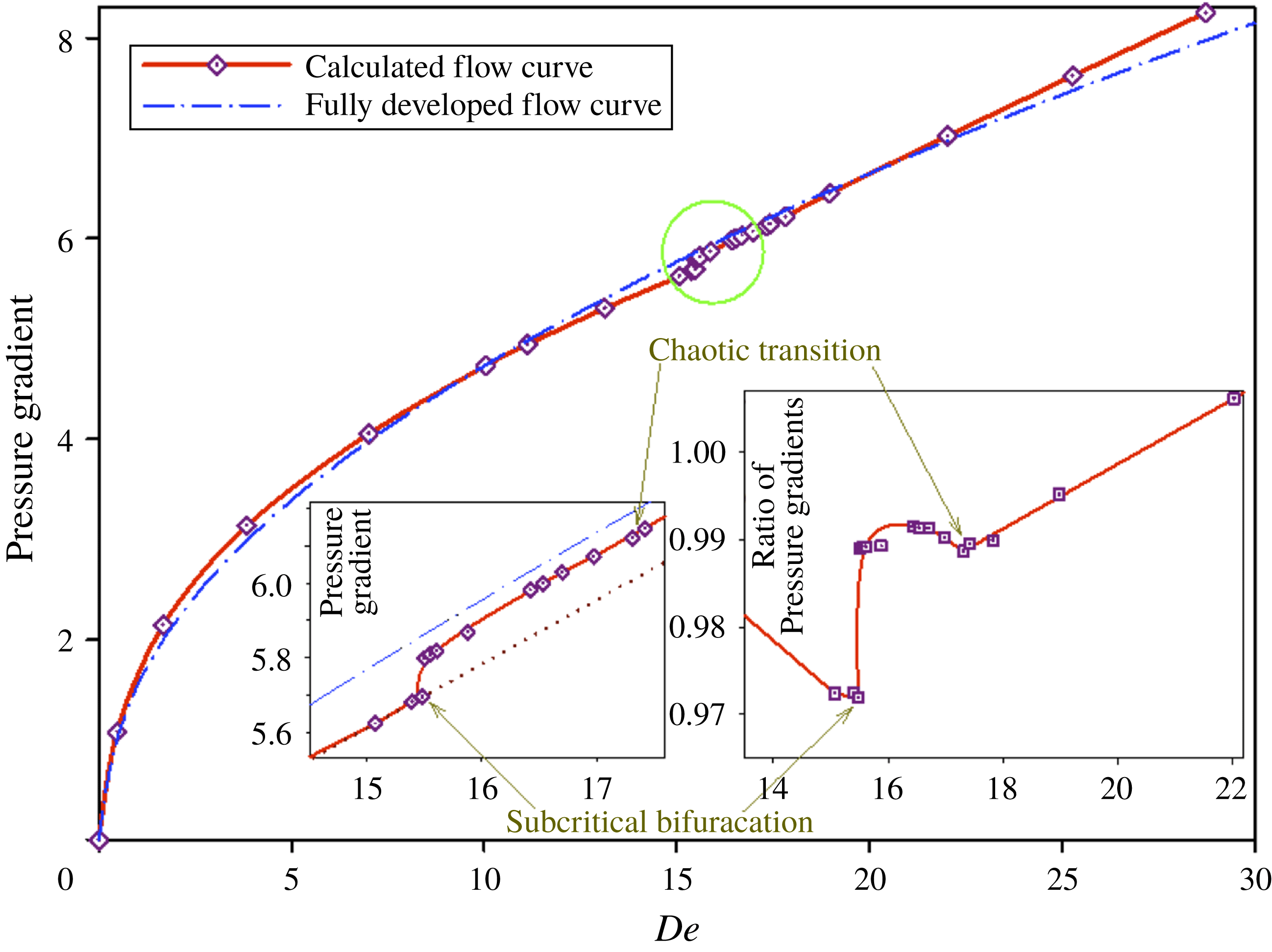
Calculated flow curve (
 $De$
versus
 $\unicode[STIX]{x0394}p/\unicode[STIX]{x0394}x$
in red with symbols) and the corresponding curve for fully developed steady flow of the straight channel (in blue dash-dot). The left inset is a magnified view of the curves inside the green circle. The right inset is the ratio between the corresponding values for the calculated and fully developed flow curves.
 $\unicode[STIX]{x0394}p$
is the time-averaged pressure difference in the channel exit region (
 $\unicode[STIX]{x0394}p=p(x=-6)-p(x=0)$
and thus
 $\unicode[STIX]{x0394}x=6$
).
Modified flow curve of
 $De$
versus
 $(\unicode[STIX]{x0394}p/\unicode[STIX]{x0394}x)-(c_{1}\times De+c_{2})$
calculated from the hysteretic flow analysis by slowly decreasing
 $De$
from the solution at
 $De=15.55$
(red curve) and slowly increasing
 $De$
from the solution at
 $De=15.07$
(blue dashed curve). Green and blue solid curves represent solutions for steady and fully developed unstable flows, respectively.
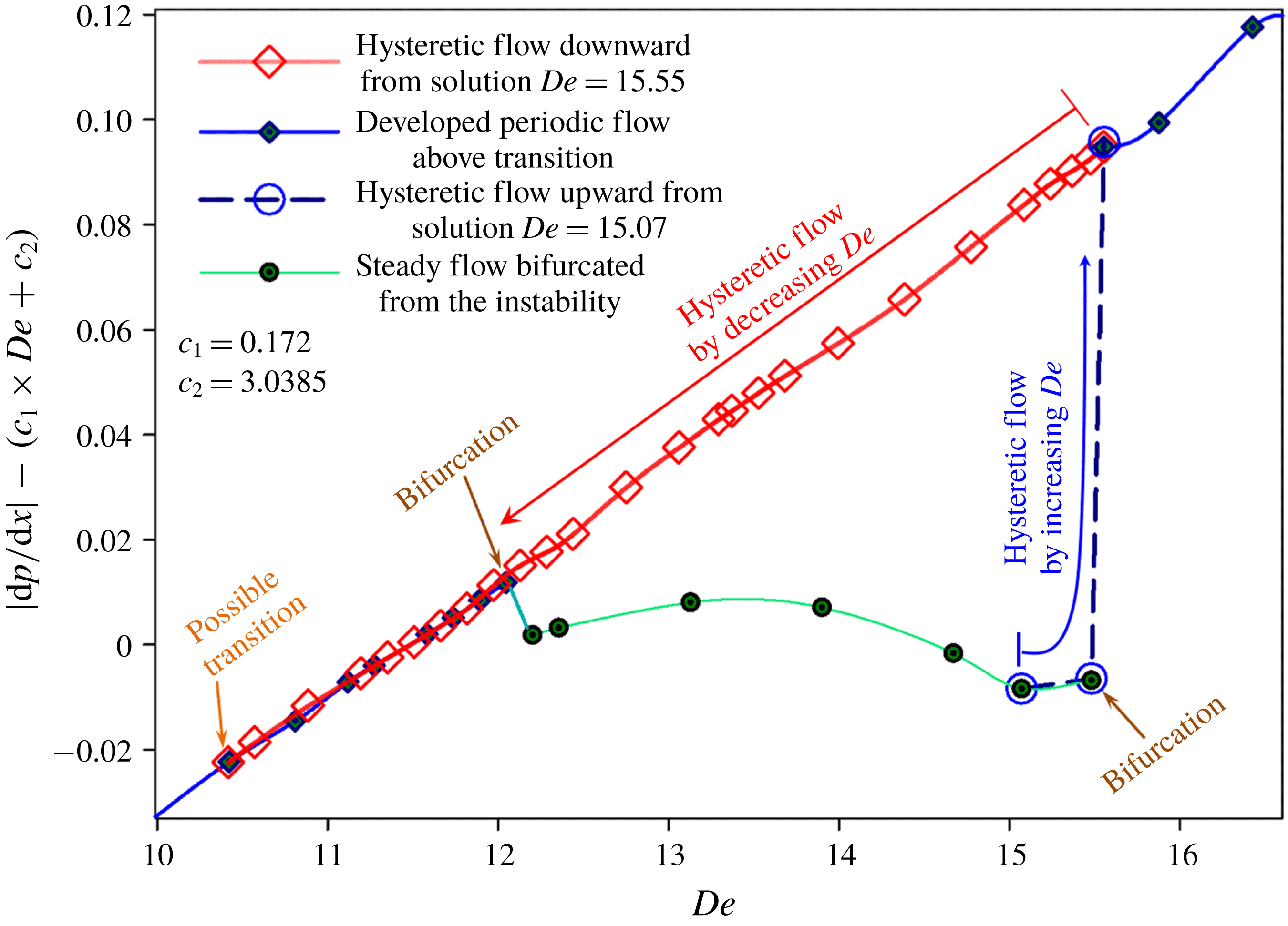
Figure 4 showing the dependence of the pressure gradient on
 $De$
, may elucidate the nature of dynamic flow transition explicitly, where the red curve with symbols represents the pressure gradient
 $-\text{d}p/\text{d}x$
(time averaged in the case of instability) calculated for the channel end region of length 6 (i.e. in the region
 $-6<x<0$
) and the equivalent curve in the fully developed steady flow of a straight die is also shown by the blue dash-dot curve for comparison. The solution expresses overall downward concavity, especially in the region
 $De<7$
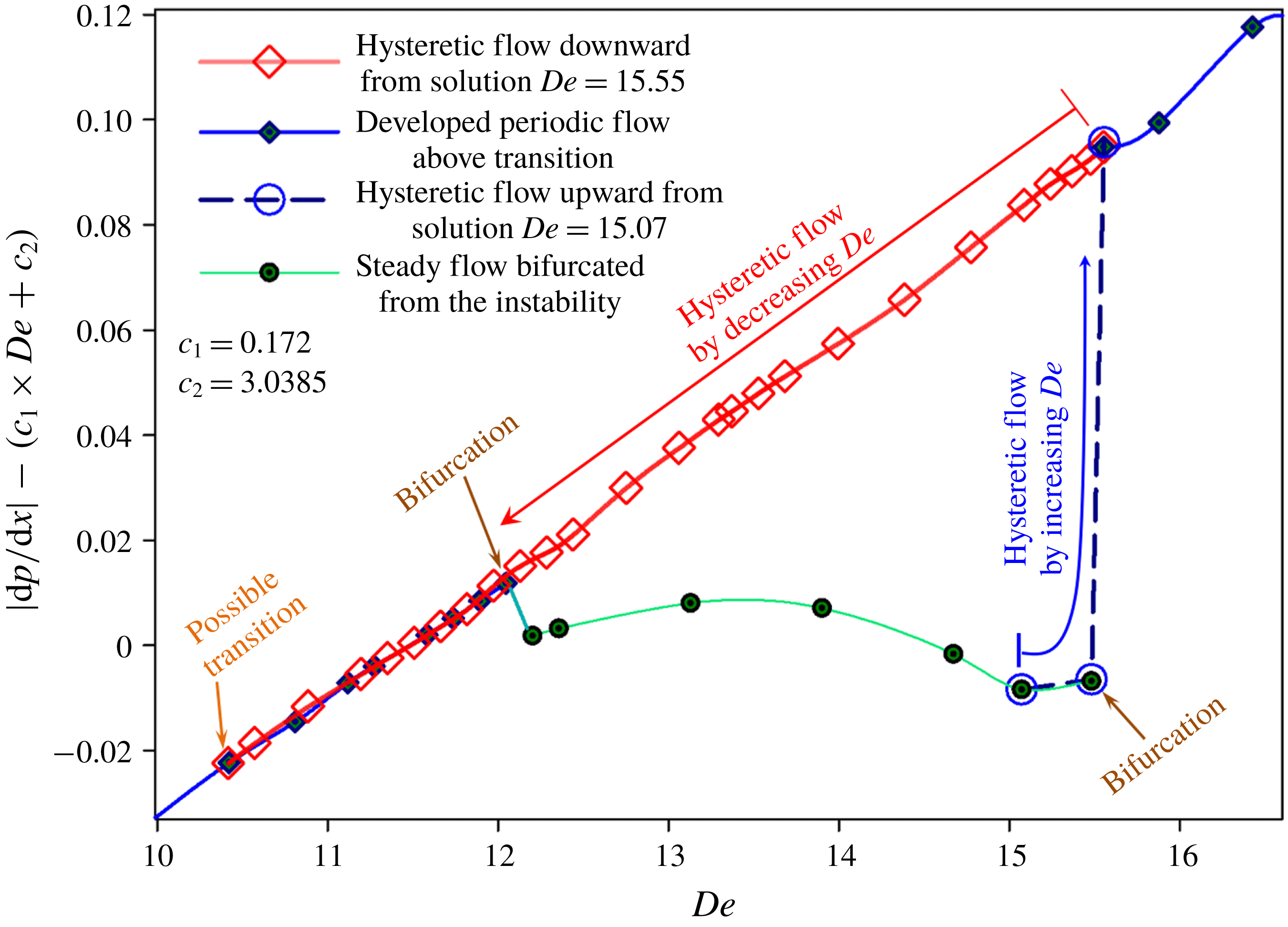
, which is chiefly incurred by the shear thinning characteristic inherent in the Leonov constitutive equation. On the other hand, careful examination of the red flow curve confirms bifurcations noted as functional or differential discontinuities and also several crossings with the blue curve that indeed originate from the dynamic transition of flow regimes. The magnified detail of the graph inside the green circle is redrawn in the left figure inset, and even if small in magnitude, the discontinuous jump in the flow curve deduced as the subcritical bifurcation is clearly indicated at
 $De=15.5$
, which denotes the transition from a time-invariant steady solution to the periodic limit cycle (the sharkskin instability of the extrudate). More precisely, a very small fluctuation indeed starts near
 $De=10.4$
, where its existence is evident, but due to extremely slow development into instability and weakness of the fluctuation signals, its correct identification is very difficult and thus the detailed analysis is not included in the current study. When we further increase
 $De$
in this start-up flow simulation, another peculiar transition from a periodic limit cycle to a stable steady flow emerges at
 $De=12.1$
. Then, as soon as
 $De$
exceeds the critical value
 $De=15.5$
, the second periodic instability appears and the amplitude of fluctuations for
 $Q_{asym}$
becomes approximately 20 times larger than that of the previous fluctuation with
 $De<12.1$
(here all the points are obtained from the steady solution or the time average of the fully developed instability initiated as a start-up flow). The apparent loss of continuity of data at the transition of
 $De=15.5$
results from the subcritical dynamic transition concluded from the hysteretic flow simulation exhibited in figure 5. Therefore, this subcritical Hopf bifurcation transforms the second steady flow again into the periodic limit cycle presumed herein as the sharkskin melt fracture.
Concerning the result interpreted as the sharkskin instability, a rather critical remark should be made. This instability may be associated with a type of melt fracture distinct from sharkskin fracture, that is, in the real 3-D case it may represent a spiral pattern of melt fracture or another 3-D periodic kind of unstable flow. In the study of 2-D flow we cannot identify its exact type and evidently this expresses the limitation of the 2-D flow simulation. Notwithstanding the unavoidable uncertainty, this melt fracture with periodic fluctuations of relatively small amplitude is termed the sharkskin instability, which seems the most appropriate choice with the current restricted amount of information.
The right inset of figure 4 replots the flow curve of the pressure gradient divided by the value corresponding to fully developed steady flow (the blue curve), which more sensitively detects the conversion of the dynamics. In addition to the subcritical bifurcation, there discernibly exists another transition at
 $De=17.3$
, which leads to chaotic flow converted from the quasiperiodic regime, and it is expressed as an abrupt slope change which is not clear in the left inset of the normal flow curve but is in the right inset of the modified plot. Past this transition, there appears a crossing of the blue and red curves near
 $De=20$
(in the main figure), which means that, owing to this instability, the power required for unstable flow begins to exceed that for the corresponding developed steady flow of a straight die. The current phenomenon is similar to that present in the turbulence of a Newtonian fluid although a strict analogy unquestionably necessitates flow modelling of 3-D elastic turbulence which is not the subject of this paper.
According to the current result combined with past research results reported elsewhere, it is concluded that there possibly exist two competing mechanisms for sharkskin fracture; the subcritical transition herein suggested and the wall slip near the die lip. In principle, a distinction between them can be made in experiments even though this may be hard in practice. If the sharkskin is initiated by the wall slip, then the slope of the flow curve (the common flow curve of pressure drop versus apparent shear rate, or the current flow curve of pressure gradient versus
 $De$
) would decrease at the transition due to reduction of the wall shear rate (and thus decrease in wall shear stress) in comparison with the nominal one. On the other hand, in the case of sharkskin fracture caused by the subcritical bifurcation described in this study, the apparent slope would slightly increase due to a small discontinuous jump, as shown in figure 4, since inducing temporally periodic behaviour is presumed to necessitate an extra pressure drop. However, this kind of subtle change in the slope of the flow curve may be easily hidden in comparison with the overall behaviour of total pressure variation along the entire flow channel measured experimentally, and thus its detection may be hard in practice.
In order to certify more convincing evidence for subcritical transition, a curve of flow hysteresis is shown in figure 5 by slowly decreasing
 $De$
(the decreasing direction denoted with a red arrow) from the developed periodic flow at
 $De=15.55$
as the initial value, where the solution consists of the unstable state corresponding to sharkskin fracture just above the subcritical transition. In more detail, the inlet boundary located at
 $x=-20$
was assigned steady Poiseuille flow profile for the straight pipe corresponding to a desired
 $De$
slightly lower than the previous setting. Then the computation was started from the previous fully developed solution until a new fully developed instability or fully relaxed steady state was attained. This process continued up to a
 $De$
as low as 10.4 and the solution is drawn as the red curve with empty diamond symbols while the original solution of start-up flow is given with the blue curve and filled symbols. For clear illustration, the values of the ordinate are modified by subtracting the linear regression line (regression of data for the lower branch steady flow from
 $12.1<De<15.5$
) from the pressure gradient, that is, the vertical axis assigns values of
 $|\text{d}p/\text{d}x|-(c_{1}\times De+c_{2})$
where
 $c_{1}=0.172$
and
 $c_{2}=3.0385$
. The red curve distinctly exhibits flow hysteresis, that is, the current system contains multiple solutions in the range of
 $12.1<De<15.5$
, where the lower branch (lower green curve) expresses a steady flow solution but the upper branch (red curve) corresponds to a periodic sharkskin melt fracture.
The lower branch solution of steady flow (green symbols with a green curve) is obtained when the start-up flow simulation from the rest state explained in § 2 is performed or the test of hysteresis initiated from the steady branch itself (solution corresponding to the lower branch for
 $12.1<De<15.5$
) is carried out. However, the upper branch of unstable periodic solution (red diamond symbols with a red curve in
 $12.1<De<15.5$
) is attainable only in the case of a hysteretic flow simulation starting from the unstable periodic solution (the upper branch solution itself or the developed unstable flow solution for
 $De>15.5$
). On the other hand, although the simulation starts from the lower branch of the steady state, the solution enters again into weak periodic instability when the
 $De$
is set lower than 12.1 by the decrease of flow rate. This weak fluctuation persists at a
 $De$
as low as 10.4, and then the flow becomes steady and stable as
 $De$
further decreases below 10.4. In the unstable domain with periodicity
 $(10.4<De<16)$
, the amplitude of the fluctuations continuously decreases with
 $De$
decreasing in the direction of red arrow in the figure. Unlike the typical subcritical transition, below
 $De=15.5$
there has not been observed any abrupt change (the discontinuous jump at the saddle-node point from the upper to the lower branch) on the hysteresis curve on decreasing
 $De$
, and this is suspected to result from unresolved complex dynamics initiated at two bifurcations at
 $De=10.4$
and 12.1. The existence of the lower branch solution of steady state in the middle of periodic instability is quite unique and peculiar, and thus its further investigation, including the identification of the bifurcation at
 $De=10.4$
, suggests a good subject of future study.
For more detailed analysis, an additional curve of flow hysteresis in the opposite sense has also been obtained by slowly increasing
 $De$
from the solution on the lower branch at
 $De=15.07$
(the increasing direction denoted with blue arrow in figure 5), where this initial condition is the solution corresponding to fully relaxed steady flow below the subcritical transition. The solution is drawn as the blue dashed curve with large circular symbols. In this numerical test on the other hand, an abrupt discontinuous jump of pressure gradient is markedly recognizable near
 $De=15.5$
, where an increase of
 $De$
as small as 0.45 % (from 15.48 to 15.55 in terms of
 $De$
) brings about the rather large step variation illustrated in the figure. This is equivalent to the discontinuous jump already observed in the curve of the start-up flow simulation from rest shown in figure 4 and confirms the subcritical bifurcation involved in the nonlinear flow dynamics leading to periodic melt fracture. When one takes into consideration the result of supercritical bifurcation demonstrated experimentally (Arratia et al.
Reference Arratia, Thomas, Diorio and Gollub2006) and computationally (Poole et al.
Reference Poole, Alves and Oliveira2007) in the elongation dominated cross-slot flow, two bifurcations at
 $De=10.4$
and 12.1 in addition to the subcritical one at 15.5 as well as the chaotic transition at 17.3 herein associated with melt fracture signify the complexity and variety of nonlinear dynamic phenomena possibly present in elastic flow instability.
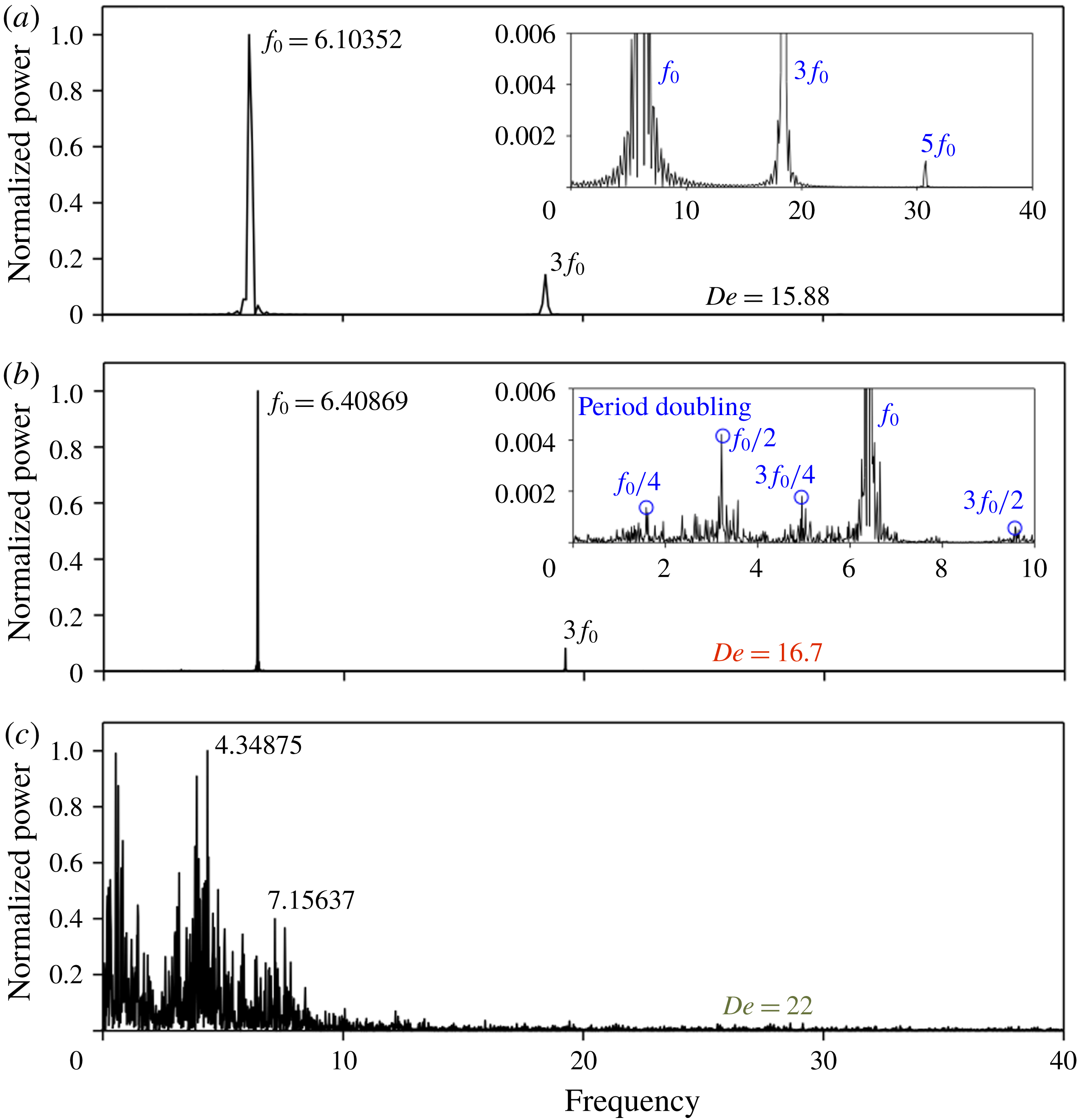
FFT spectrum (power normalized by the amplitude of maximum peak). Figure insets are the magnifications of the spectrum that illustrate the main and subharmonic peaks: (a)
 $De=15.88$
, (b)
 $De=16.7$
, (c)
 $De=22$
.
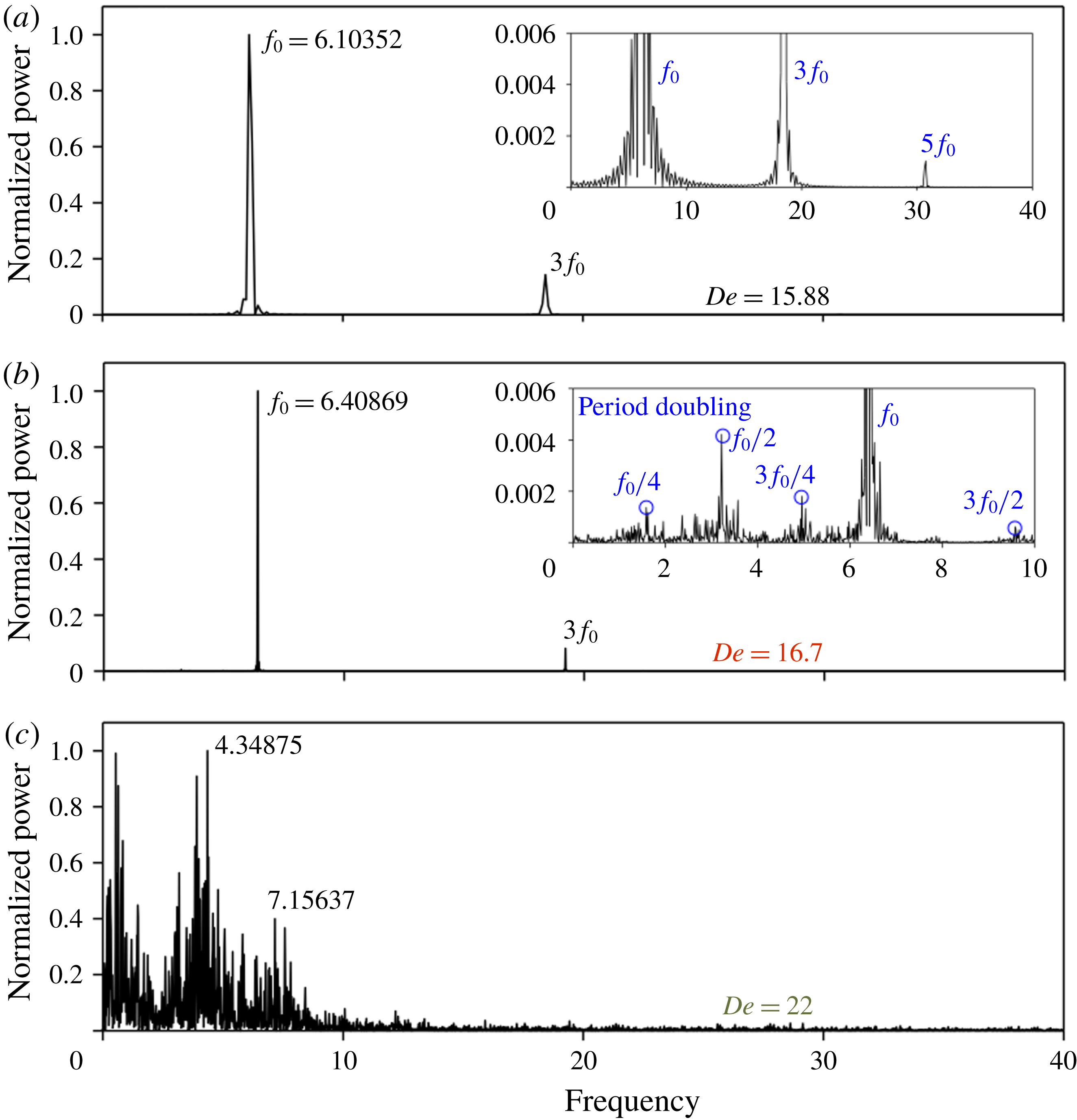
The time-dependent function
 $Q_{asym}$
of figure 3 is transformed into a frequency spectrum in figure 6 by fast Fourier transform (FFT), where the amplitude is normalized by the magnitude at the maximum peak. In the perfectly periodic case of
 $De=15.88$
, distinct modes at
 $f_{0}$
and at odd multiples of
 $3f_{0}$
and
 $5f_{0}$
are observed and essentially no other frequency modes exist, which can be clearly seen in the inset of figure 6(a). As the flow rate increases to
 $De=16.7$
, the main mode slightly shifts to higher frequency and small peaks of subharmonic modes appear at integral fractions of the main and odd multiple frequencies, which are denoted in the inset of figure 6(b) as peaks marked with small blue circles. These small amplitude modes seem to show signs of period doubling bifurcation (doubling at
 $f_{0}/2$
and
 $3f_{0}/2$
; quadrupling at
 $f_{0}/4$
and
 $3f_{0}/4$
). Other smaller peaks probably indicate signs of quasiperiodic transition with the appearance of incommensurate subharmonic motions in the flow dynamics. Figure 6(c), on the contrary, evinces a densely distributed frequency spectrum, especially the slow mode appears with notable amplitude, and thus this offers an affirmative proof of the chaotic dynamics involved in the flow. In turn, figure 6(b) provides evidence of chaotic (figure 6
c) transition through period doubling as well as a quasiperiodic route from a limit cycle (figure 6
a).
At this point several comments should be made. The current subcritical bifurcation from the steady (shown by the extrudate profile portrayed in figure 1) to periodic flow state of figure 3(a) is specifically distinguished from the subcritical route to melt fracture observed in other studies (Bertola et al.
Reference Bertola, Meulenbroek, Wagner, Storm, Morozov, van Saarloos and Bonn2003; Meulenbroek et al.
Reference Meulenbroek, Storm, Bertola, Wagner, Bonn and van Saarloos2003). On frequent occasions, the real extrudate instability starts in a periodic form of sharkskin fracture depicted in figures 3(a) or 6(a) presumably by way of the subcritical transition, and then, as the flow rate or
 $De$
further increases, various types of large amplitude melt fracture emerge, one of which belongs to the gross melt fracture (cf. Leonov & Prokunin Reference Leonov and Prokunin1994). The gross melt fracture is thought to result mainly from the other type of subcritical instability generated by the intense flow inside the die (Meulenbroek et al.
Reference Meulenbroek, Storm, Bertola, Wagner, Bonn and van Saarloos2003) or the spurt flow (Adewale & Leonov Reference Adewale and Leonov1997). However, this study suggests additional instance of its occurrence via the chaotic transition depicted in figures 3(c) and 6(c) as long as the finite disturbance remains sufficiently small to prohibit the subcritical bifurcation along the die and thus, under no-slip conditions, the dynamics takes the route of period-doubling/quasiperiodic transition to chaos. Without wall slip taken into account (by the assumption made here), the die lip singularity becomes the sole origin of melt fracture in this work. At the end tip of the channel wall, the finite curvature of the streamlines results from the sudden expansion of the flow stream, and furthermore, the abrupt change of boundaries from no-slip on the wall to the free surface of the extrudate causes concentrated extension of liquid elements and accordingly high tensile stress. As a result, this further intensifies the singular character of the die exit wall. This unavoidable streamline curvature even induces tiny vortices attached to the die lip, which readily lose stability and start to fluctuate under high stress, and this is thought to give rise to nonlinear instability via the chaotic transition as well as subcritical bifurcation at some critical
 $De$
. Such vortices rarely or weakly appear in the steady state, however in the unstable regime they are manifestly formed and oscillate with periodic, quasiperiodic or aperiodic duration (snapshots on the left of figure 3 portray such tiny vortices with high pressure gradients near the exit wall and their chronological dynamics can be observed in the animation of supplementary movies).
Actually, the main result of this section does not consist of the complete verification of the complicated mechanism of sharkskin and melt fracture instability. To the contrary, we assert that description or analysis of sharkskin fracture based on the fundamental assumption only of wall slip may be misleading and has to be incorporated with the current nonlinear dynamic mechanism, since both mechanisms, wall slip and nonlinear dynamic transition (subcritical or chaotic bifurcation), will compete for the initiation and further evolution of sharkskin instability. In other words, this work proves a possibility that even without any wall slip almost every kind of melt fracture can be realized simply in terms of the high stress along the curved streamlines near the die lip. Although the mechanism is not certain yet, the wall slip may become the most crucial element determining the onset of sharkskin. Nevertheless, when rigorously and realistically modelling melt fracture, one has to consider the problem based on a slip boundary, including all the nonlinear dynamics herein performed.
3.2 Effect of geometrical exit modification on melt fracture
In this section, we examine the effect of geometrical modification of the die exit domain on melt fracture, especially on the sharkskin instability. Since the occurrence of melt fracture instability usually sets the upper bound of manufacturing speed, in the real industrial process, the control of melt fracture or delay of the onset of sharkskin is valuable. In the current geometry of a straight channel under Poiseuille flow, the die lip, that is, the end point of channel wall, becomes the sole origin of sharkskin or melt fracture under the boundary condition specified as no slip. These lip points in the mathematical approximation of the elastic flow designate a strong singularity where the flow boundary abruptly changes from no slip to free surface and, accordingly, intense extensional deformation exists. Introducing a short expansion channel element at the tip of the die we make an attempt to attenuate the degree of strength of the die lip singularity. For this purpose, a basic computational domain with no expansion element is constructed with triangular mesh elements that are not symmetric about the centreline (line of
 $y=0$
), as shown in figure 2(b), in order to examine whether the introduction of the exit modification can recover the flow symmetry even in an asymmetrically discretized flow domain. A short expansion flow domain is introduced with a length of
 $H/2$
(i.e. in the region of
 $-0.5<x<0$
) and variable slope, and one example of the modified channel domain is exhibited in figure 2(c), where the slope of channel exit is 0.34 (
 $-0.34$
for the lower wall). As before, every wall of the channel, including the diverging wall elements, is assigned as a no-slip boundary, and therefore the following results for the flow field, instability and possible stabilization induced by this die modification are valid and meaningful only under the current computational regime of strictly no slip.
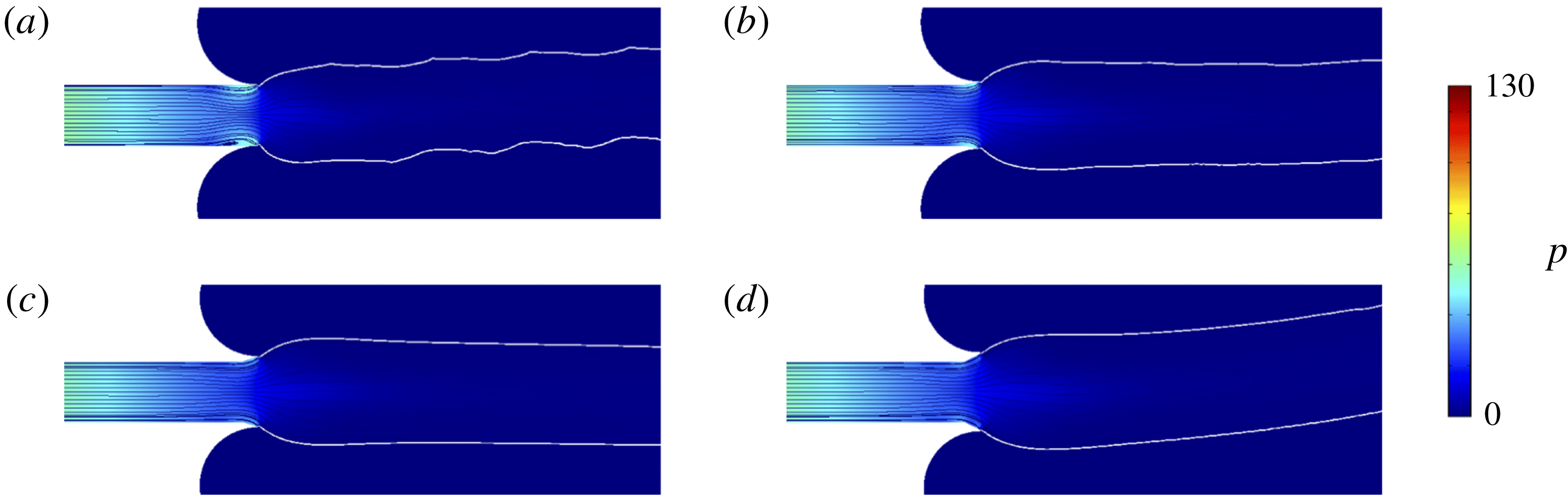
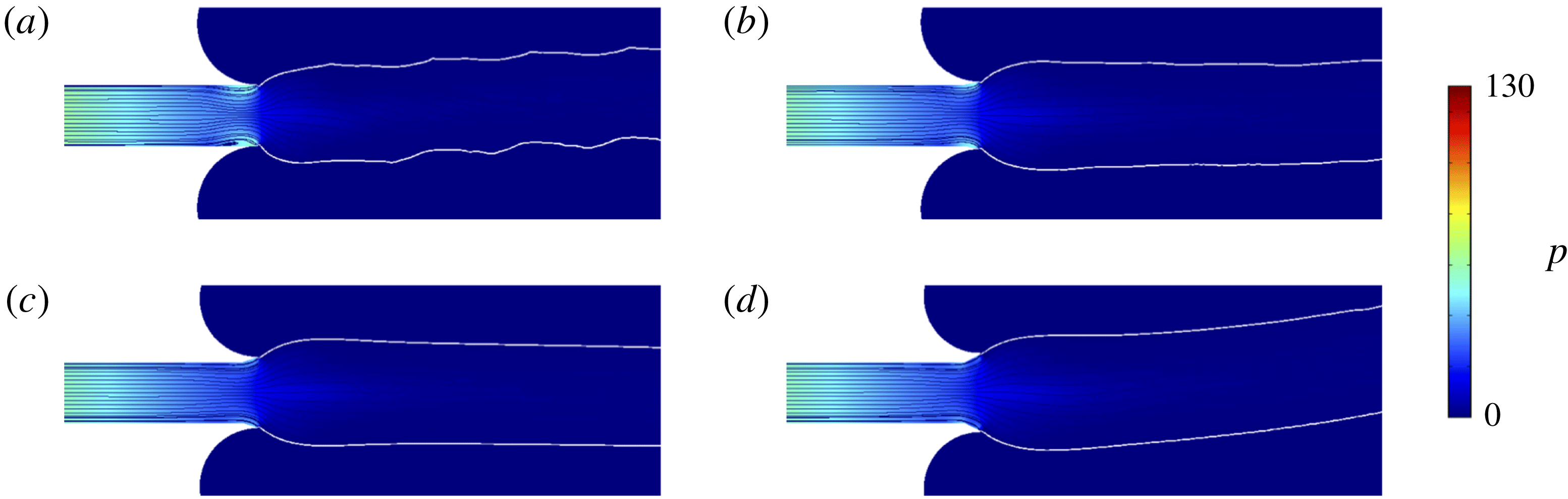
As an example, the flow at
 $De=16$
is computationally modelled with the asymmetric mesh of figure 2(b) and the resultant extrudate profile with streamlines and pressure contour is drawn in figure 7(a) at the instant
 $t=5$
. The elastic flow instability consists in a domain of periodic sharkskin occurring above the subcritical transition, however, in addition, the extrudate displays overall skewness (that is, the computed extrudate profile is bent upwards) possibly due to an artefact of the asymmetric discrete spatial resolution. Figure 7(b–d) illustrates at the same temporal instant the results for the modified exit geometry, which demonstrate the dependence of the interface evolution on the slope of diverging wall and the general tendency of decreasing sharkskin for the introduction of this expansion channel element. Such a diminishing amplitude of fluctuation notwithstanding, the case of figure 7(b) (slope 0.2) still exhibits a rough interface due to the remaining unstable flow dynamics and figure 7(d) (slope 0.5) shows the skewness remaining in the extrudate liquid. On the other hand, figure 7(c), of slope 0.34, depicts a smooth interface as well as an extrudate symmetry that is almost recovered.
A similar analysis has been performed with the equivalent spatial approximation for
 $De=22$
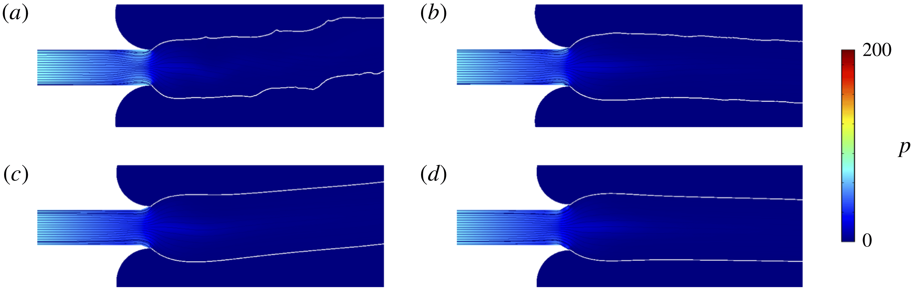
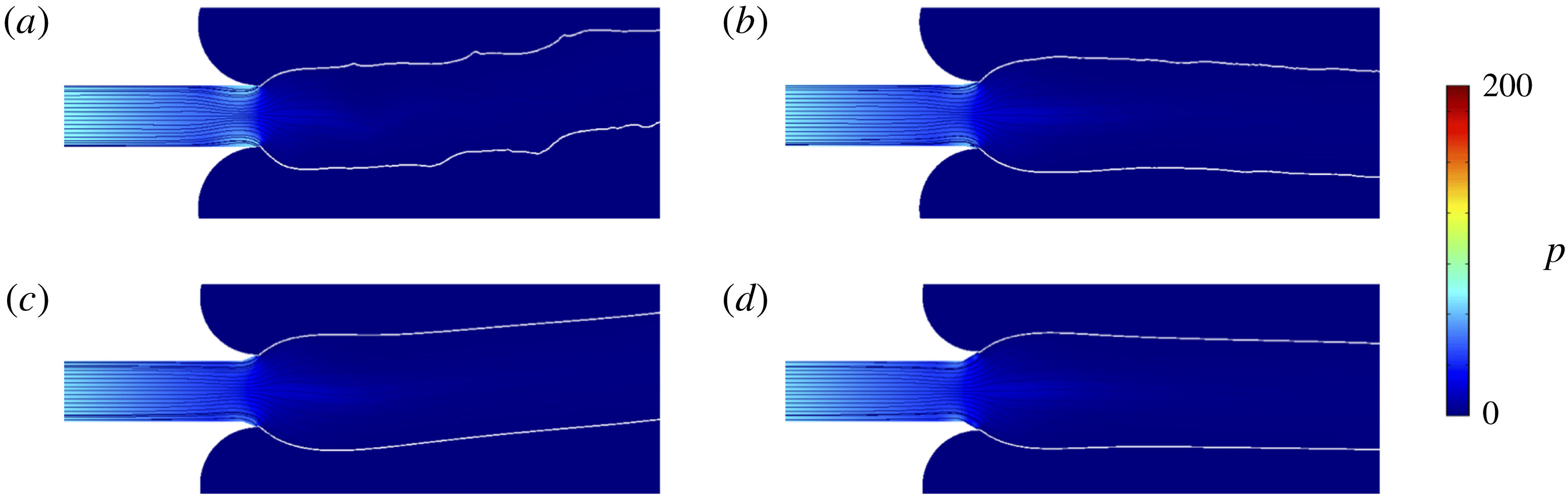
, in which the unstable flow corresponds to the chaotic regime. Figure 8 represents the solution at
 $t=2$
for the exit wall slope (a) 0 (i.e. no exit modification), (b) 0.2, (c) 0.4 and (d) 0.6. As a result, figure 8(a) obviously presents the surface profile corresponding to gross melt fracture. Even under this heavy elastic effect, the introduction of a short expansion channel at the exit dramatically alleviates the instability, which can be observed in figure 8(b–d). Especially the channel part of slope 0.6 (figure d) is shown to be the most effective at recovering an almost symmetric and smooth profile.
Streamlines and extrudate surfaces on the contour of pressure at
 $t=5$
and
 $De=16$
: (a) original flow domain without die exit modification, and flow domain with exit modification of slope of exit wall: (b) 0.2, (c) 0.34, (d) 0.5.
Streamlines and extrudate surfaces on the contour of pressure at
 $t=2$
and
 $De=22$
: (a) original flow domain without die exit modification, and flow domain with exit modification of slope of exit wall: (b) 0.2, (c) 0.4, (d) 0.6.
Although it is at this stage too early to estimate the practical efficiency and to draw conclusions, the current study verifies that the geometrical modification of the channel exit wall has a drastic influence on the flow dynamics and instability leading to melt fracture. Now that notable wall slip may occur in the chaotic instability, the effect of the diverging wall element is doubtable for the reduction of gross melt fracture. However, in the weakly unstable flow exhibiting sharkskin, this channel modification is judged to be feasible. Indeed, the removal or reduction of the sharkskin melt fracture has been experimentally observed by the introduction of a diverging taper at the die exit similar to that of the current modelling (Pol et al. Reference Pol, Joshi, Tapadia, Lele and Mashelkar2007). Whereas this numerical outcome, supported by experimental evidence of Pol et al. (Reference Pol, Joshi, Tapadia, Lele and Mashelkar2007), suggests the potential feasibility of die exit modification, the expansion channel could possibly raise the degree of extrudate swelling and thus this apparent improvement may simply amount to stable flow through a wider channel where sharkskin disappears due to lowered shear strength. In addition, the following needs to be mentioned: the experimental verification by Pol et al. (Reference Pol, Joshi, Tapadia, Lele and Mashelkar2007) may not be regarded as a strict proof for the validity of the instability mechanism provided by the current analysis since the sharkskin caused by wall slip may also be reduced in the modification into the diverging die.
4 Conclusions
In this study, we first made an attempt to computationally describe the extrudate surface undulation initiated into a form of periodic sharkskin in the current setting of flow dynamics with no-slip boundary conditions. The nonlinear dynamics involved in this instability is shown to be quite complicated. The first bifurcation from a stable steady state at
 $De=10.4$
results in a weak periodic fluctuation of the flow field, and then at
 $De=12.1$
this periodic limit cycle bifurcates into another stable steady flow, coexistent with the instability. Then, a subcritical transition of the steady solution returning to the limit cycle is manifested at
 $De=15.5$
. Therefore, in the middle of flow instability, the unique coexistence of multiple solutions such as the second stable steady flow and the periodic limit cycle has been elucidated. With the further increase of
 $De$
, the flow enters the state of 2-D chaos at
 $De=17.3$
presumably taking the period-doubling/quasiperiodic route. As a practically useful analysis, control of melt fracture by the geometrical modification of the channel exit element is also undertaken in this numerical modelling, and it is shown that the introduction of a diverging exit wall drastically reduces elastic flow instability. The mechanism of flow transitions is verified with nonlinear dynamics taken into account (the preliminary analysis of nonlinear dynamic data in terms of pseudo time series analysis or the method of embedding dimension can be found in Appendix) and we infer the origin of the onset of melt fracture as the sharkskin instability, which consists of nonlinear instability due to the transition by high stress along curved streamlines near the exit wall singularity. However, in the real flow situation, the subcritical instability inside the channel or the spurt (stick-slip on the wall) phenomenon may intervene in the current scenario of flow dynamics. In practice, we conclude that the subcritical bifurcation herein caused by the die lip singularity and wall slip transition at the die exit will determine the onset of sharkskin instability. On the other hand, the subcritical transition of the flow along the channel and large-scale slip (and possibly chaotic transition found in this study) seem to mainly control gross melt fracture or spurt phenomenon. Therefore, if one incorporates the current modelling with a proper methodology of wall slip, a realistic and complete description of melt fracture would become possible and this will be the subject of future study.
Acknowledgements
The research was supported by Basic Science Research Program through the National Research Foundation of Korea (NRF) funded by the Ministry of Science, ICT and Future Planning (NRF-2017R1A2B4006278).
Supplementary movies
Supplementary movies are available at https://doi.org/10.1017/jfm.2018.659.
Appendix
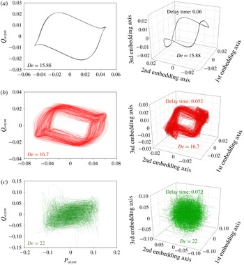
Two-dimensional phase planes (left) and 3-D phase space portraits (right): (a)
 $De=15.88$
, (b)
 $De=16.7$
, (c)
 $De=22$
.
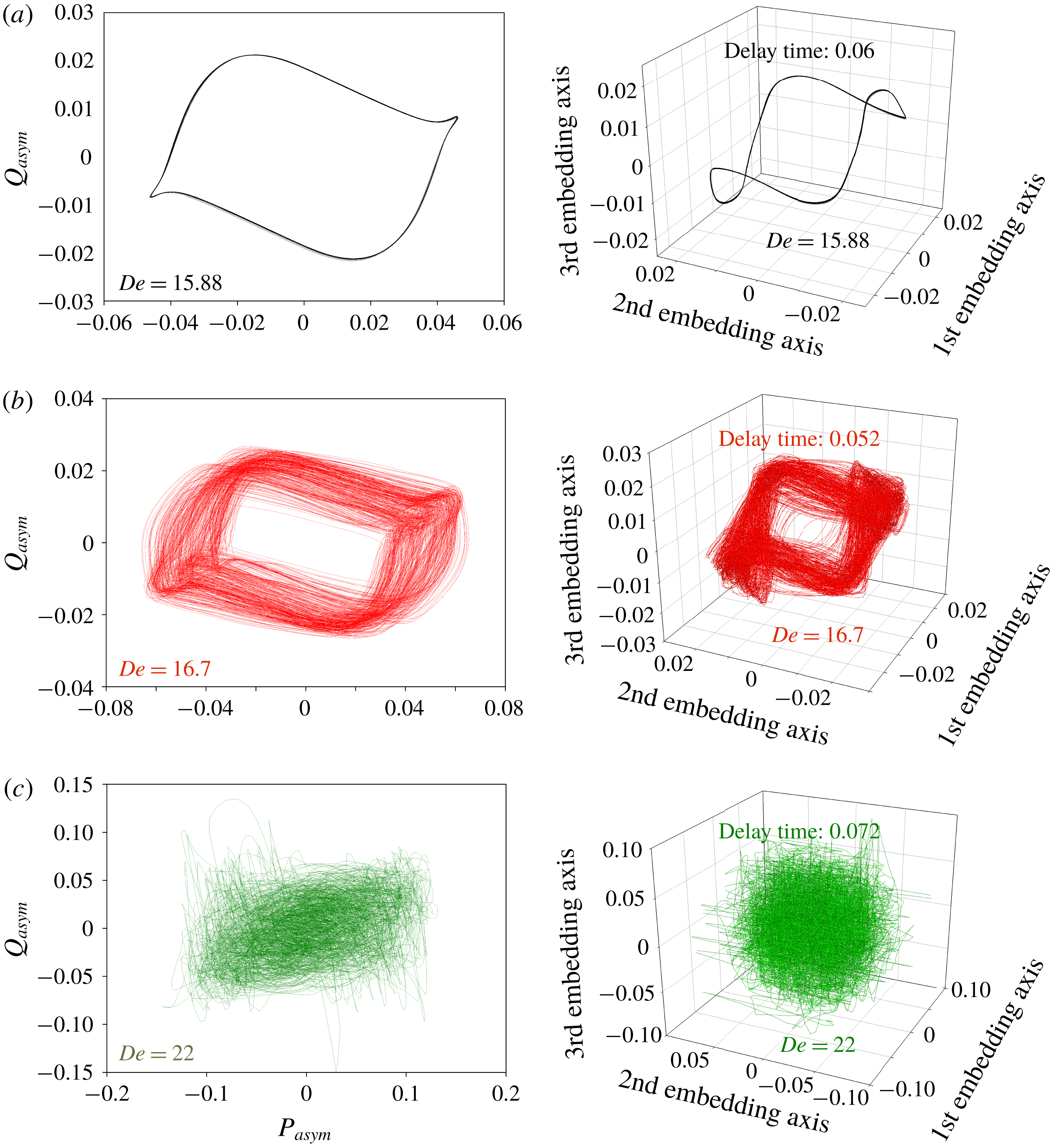
This appendix discusses the preliminary analysis of nonlinear dynamic data from the computational results for melt fracture that may buttress the conclusion drawn in the main text. Herein two sets of data for
 $Q_{asym}$
and
 $P_{asym}$
are employed, where
 $Q_{asym}$
is chosen as the primary variable (defined in the main text) and
 $P_{asym}\equiv (\unicode[STIX]{x0394}P_{up}--\unicode[STIX]{x0394}P_{low})/(\unicode[STIX]{x0394}P_{up}+\unicode[STIX]{x0394}P_{low})$
. Their time series are collected from numerical calculation to quantitatively express the dynamic instability represented as temporal flow asymmetry.
 $\unicode[STIX]{x0394}P_{up}$
and
 $\unicode[STIX]{x0394}P_{low}$
are mean pressure differences along the channel end of length 6 for upper and lower halves, respectively, i.e.
 $\unicode[STIX]{x0394}P_{up}\equiv \int _{0}^{1}[p(x=-6)-p(x=0)]\,\text{d}y$
and
 $\unicode[STIX]{x0394}P_{low}\equiv \int _{-1}^{0}[p(x=-6)-p(x=0)]\,\text{d}y$
. Since the actual dimension of the current nonlinear dynamical system is not known a priori, current analysis employs namely the method of attractor reconstruction or construction of a pseudo phase space from a single scalar time series based on the theorem by Packard et al. (Reference Packard, Crutchfield, Farmer and Shaw1980) and Takens (Reference Takens, Rand and Young1981). Before the reconstruction of single time series data, a 2-D phase plane of
 $Q_{asym}$
versus
 $P_{asym}$
is depicted in the left of figure 9 for three distinct flow rates. As described in the main text, the case of
 $De=15.88$
corresponds to the periodic state and thus the phase trajectory in figure 9(a) clearly demonstrates the limit cycle. On the other hand, the case (b) of
 $De=16.7$
and (c) of
 $De=22$
delineate quasiperiodic and chaotic trajectories, respectively.
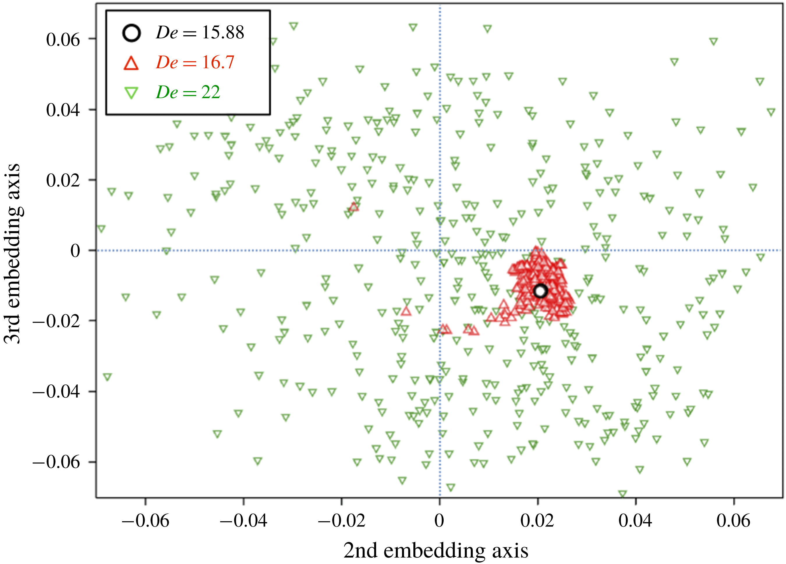
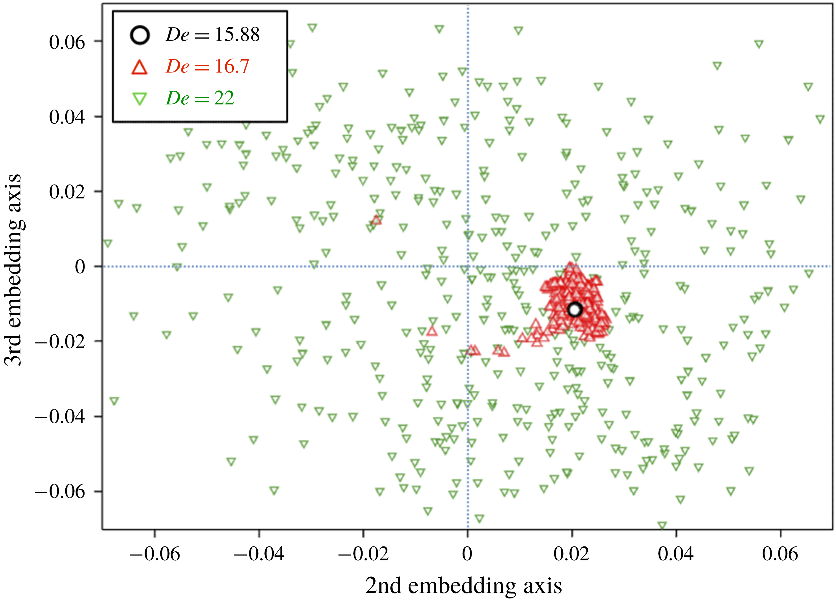
Poincaré sections for cases of
 $De=15.88$
, 16.7 and 22.
From the 1-D scalar time series data of
 $Q_{asym}$
we determine the delay times in order to artificially separate independent variables, employing so called the mutual information method (Kodba, Perc & Marhl Reference Kodba, Perc and Marhl2005). The resultant delay times for each case are in the range of 0.05–0.07 shown in figure 9 and corresponding 3-D phase space portraits drawn according to thereby derived three independent variables are given on the right of the figure. One can observe at least qualitative equivalence between the trajectories on the 2-D phase plane (left of figure 9) and the 3-D phase space (right of figure 9).
After constructing the 3-D phase space, with a proper cross-section taken through it, one may be able to build up the Poincaré map that succinctly expresses the nonlinear dynamic information of the system. Here we have chosen the plane composed of the second and third axes and in figure 10 plotted crossing points of trajectories that penetrate the plane upward. On this Poincaré section the limit cycle (the case of
 $De=15.88$
) collapses into a single point (the symbol of a open black circle), and the quasiperiodic orbits of
 $De=16.7$
represent somewhat scattered points of red triangles, while the chaotic flow state of
 $De=22$
portrays widespread distribution of points (green inverted triangles) on the plane. If more data points are available, the cases of quasiperiodic and chaotic flow systems may express complex orbital and fractal structures on the Poincaré map, respectively. Indeed, at this moment it is too hasty to draw a conclusion based on this map due to blurring by numerical error, insufficiency of data points and heavy requirement of computation time, and thus this will be a good subject of the future study.