


1 INTRODUCTION
A policy maker must decide between implementing a new policy or preserving the status quo. Her data provide information about the potential benefits of these two options. Unfortunately, these data only partially identify payoff-relevant parameters and may therefore not reveal, even in large samples, the correct course of action. Such treatment choice problems with partial identification have recently received growing interest (e.g., see D’Adamo, Reference D’Adamo2021, Ishihara and Kitagawa, Reference Ishihara and Kitagawa2021, Yata, Reference Yata2021, Christensen, Moon, and Schorfheide, Reference Christensen, Moon and Schorfheide2026, Kido, Reference Kido2022, or Manski, Reference Manski2025). Several interesting problems that arise in empirical research can be recast using this framework. See Montiel Olea, Qiu, and Stoye (Reference Montiel Olea, Qiu and Stoye2026) and the end of this section for references.
This article applies the robust Bayes approach—which interpolates between Bayesian and agnostic minimax analyses by evaluating minimax risk over a set of priors—to a class of treatment choice problems with partial identification. The use of the robust Bayes approach has drawn recent attention in problems that feature partial identification (Giacomini and Kitagawa, Reference Giacomini and Kitagawa2021; Giacomini, Kitagawa, and Read, Reference Giacomini, Kitagawa and Read2021; Christensen et al., Reference Christensen, Moon and Schorfheide2026). Indeed, due to partial identification, integrating Bayesian and minimax elements into decision making can be particularly attractive (see Poirier, Reference Poirier1998; Moon and Schorfheide, Reference Moon and Schorfheide2012, and the references therein).
The robust Bayes approach can be applied ex-ante or ex-post, depending on whether the multiple priors are used to evaluate payoffs before or after seeing the data.Footnote 1 These concepts represent two different ways of resolving model ambiguity and sampling uncertainty, and both have been proposed to improve Bayesian robustness in decision problems.
By the well-known dynamic consistency of Bayesian decision making, ex-ante and ex-post robust Bayes coincide with each other—and with standard Bayes optimality—if the set of priors is a singleton. Indeed, this equivalence is used to calculate Bayes optimal decisions in practice because ex-post rules are usually computed but ex-ante Bayes optimality is claimed. As pointed out for the present context by Giacomini et al. (Reference Giacomini, Kitagawa and Read2021), they do not in general agree otherwise.Footnote 2 However, to what extent this inequivalence affects treatment choice problem with partial identification is far from clear. The class of priors that we consider has a Cartesian product structure resembling rectangularity, a condition under which maximin welfare loss is known to be dynamically consistent.Footnote 3 While this result does not apply here—the priors are not rectangular in the strict technical sense, and the theoretical results were not established for regret loss—one might wonder if the conclusion holds anyway or else, what qualitative and quantitative relationships exist between ex-ante and ex-post robust Bayes in the presence of partial identification. Using a convenient class of priors allows us to exhaustively answer these questions in a case that we believe holds some interest.
To this end, we use the same framework as Yata (Reference Yata2021) and Montiel Olea et al. (Reference Montiel Olea, Qiu and Stoye2026) but impose a simple instance of Giacomini and Kitagawa’s
(Reference Giacomini and Kitagawa2021) set of priors, namely, a symmetric
and uniform two-point prior for reduced-form parameters and no restriction at all on
unidentified parameters given reduced-form parameters. Working with regret, we
formally define ex-ante and ex-post robust Bayes and, following Berger (Reference Berger1985), label them as “
$\Gamma $
 -minimax regret” (
$\Gamma $
 -MMR) and “
$\Gamma $
 -posterior expected regret” (
$\Gamma $
 -PER).Footnote
4
We then precisely characterize when these notions coincide and when they
disagree. The main qualitative insights are as follows:
-
• Ex-ante $\Gamma $
 -MMR and ex-post
$\Gamma $
-PER criteria do frequently disagree. This conclusion
does not hinge on whether or not randomization rules are allowed. If
randomization is permitted, the criteria differ whenever updating the
prior for the reduced-form parameter does not (ex-ante
almost surely) resolve ambiguity regarding the sign of the optimal
action. Even if randomization is not allowed, the criteria will disagree
whenever the identification power of the model (in a
sense we make precise) is sufficiently small compared to the
informativeness of the data.
-
• Randomized rules are general solution concepts in both $\Gamma $
-MMR and
$\Gamma $
-PER problems. That is, optimal rules often can or even
must randomize even if regret is evaluated ex-post. For the
ex-ante
$\Gamma $
-MMR problem, whenever the identification power of the
model is sufficiently small compared to the informativeness of the data,
(1) infinitely many optimal rules exist and (2) many of them are
randomized. For the ex-post
$\Gamma $
-PER criterion, one might conjecture by analogy to
single-prior Bayes inference that the optimal rules do not randomize.
However, as long as (1) there exists ambiguity regarding the sign of the
optimal action at the location of the two-point prior for the
reduced-form parameter and (2) randomized rules are allowed, the optimal
rule is unique and is randomized. Hence, exclusion of randomized rules
is with loss of generality and cannot be justified by simply evaluating
regret ex-post—it must come from other considerations, be they
second-order preferences or logistical or convenience concerns.


Our point is not to advocate for either notion of robust Bayes criterion. We also do
not aim to solve for robust Bayes criteria for more general sets of priors as this
would get much more involved but (we suspect) not much more instructive to
illustrate the points discussed above. What we hope to illustrate is when, and how,
$\Gamma $
 -MMR and
$\Gamma $
 -PER criteria differ. We also relate these results to timing
assumptions in a fictitious game between the policy maker and an adversarial
Nature.
Several auxiliary findings might be of independent interest. First, for
$\Gamma $
 -MMR, even if we restrict the set of decision rules to be a class
of non-randomized threshold rules based on the “efficient” linear
index, the optimal threshold is not always zero. Given the apparent symmetry of the
problem, we find this feature rather surprising. Second, whenever the dimension of
the signal is larger than
$1$
 , there always exist (regardless of the parameter space and the
variance of the signals) non-randomized linear-index threshold rules (with a
threshold equal to zero) that are
$\Gamma $
 -MMR optimal (among all decision rules). This is in stark contrast
to Montiel Olea et al. (Reference Montiel Olea, Qiu and Stoye2026), in which no
linear index rule is globally minimax regret optimal if the degree of partial
identification is severe. The intuition is that the prior much reduces the state
space; the signal space then becomes so rich relative to the state space that even
linear threshold rules can effectively mimic randomization.
The literature on treatment choice with partially identified parameters has been
growing since Manski (Reference Manski2004) and Dehejia
(Reference Dehejia2005). For partial identification with
known distribution of data, Manski (Reference Manski2000,
Reference Manski2005, Reference Manski2007a) and Stoye (Reference Stoye2007) find
minimax regret optimal treatment rules. For finite-sample minimax regret results
with model ambiguity and sampling uncertainty, see Stoye (Reference Stoye2012a, Reference Stoye2012b),
Yata (Reference Yata2021), Ishihara and Kitagawa (Reference Ishihara and Kitagawa2021), and Montiel Olea et al. (Reference Montiel Olea, Qiu and Stoye2026); Kido’s (Reference Kido2023) analysis is asymptotic. Bayes and robust Bayes approaches are
analyzed by Chamberlain (Reference Chamberlain2011), Giacomini and
Kitagawa (Reference Giacomini and Kitagawa2021), Giacomini et al. (Reference Giacomini, Kitagawa and Read2021), and Christensen et al. (Reference Christensen, Moon and Schorfheide2026), among others. Earlier investigations of
ex-ante and ex-post
$\Gamma $
 -minimax estimators include DasGupta and Studden (Reference DasGupta and Studden1989) and Betrò and Ruggeri (Reference Betrò and Ruggeri1992). See Vidakovic (Reference Vidakovic2000) for a review. For different settings with point-identified
welfare, finite- and large-sample results on optimal treatment choice rules were
derived by Canner (Reference Canner1970), Chen and
Guggenberger (Reference Chen and Guggenberger2025), Hirano and Porter (Reference Hirano and Porter2009, Reference Hirano, Porter, Durlauf, Hansen, Heckman and Matzkin2020), Kitagawa, Lee, and Qiu (Reference Kitagawa, Lee and Qiu2026), Schlag (Reference Schlag2006), Stoye
(Reference Stoye2009), and Tetenov (Reference Tetenov2012b). There is also a large literature on optimal
policy learning with covariates containing results with point identified
(Bhattacharya and Dupas, Reference Bhattacharya and Dupas2012; Kitagawa and
Tetenov, Reference Kitagawa and Tetenov2018, Reference Kitagawa and Tetenov2021; Athey and Wager, Reference Athey and Wager2021; Kitagawa et al., Reference Kitagawa, Sakaguchi and Tetenov2021;
Mbakop and Tabord-Meehan, Reference Mbakop and Tabord-Meehan2021; Kitagawa and
Wang, Reference Kitagawa and Wang2023; Ida et al., Reference Ida, Ishihara, Ito, Kido, Kitagawa, Sakaguchi and Sasaki2026) as well as partially identified (Kallus and Zhou,
Reference Kallus and Zhou2018; Ben-Michael et al., Reference Ben-Michael, Greiner, Imai and Jiang2025; D’Adamo, Reference D’Adamo2021; Adjaho and Christensen, Reference Adjaho and Christensen2022; Ben-Michael, Imai, and Jiang, Reference Ben-Michael, Imai and Jiang2022; Christensen et al., Reference Christensen, Moon and Schorfheide2026;
Kido, Reference Kido2022; Lei, Sahoo, and Wager, Reference Lei, Sahoo and Wager2023) parameters. Guggenberger, Mehta, and
Pavlov (Reference Guggenberger, Mehta and Pavlov2024) and Manski and Tetenov (Reference Manski and Tetenov2023) analyze related problems but focus on
quantile, as opposed to expected, loss; Song (Reference Song2014) considers partial identification but mean squared error regret
loss.
The rest of this article is organized as follows. Section 2 sets up the problem, provides examples, and defines both versions of robust Bayes optimality. Section 3 contains complete solutions for all aforementioned scenarios and relates them to timing assumptions in the “Games against Nature” interpretation of minimax theory. Section 4 concludes. Proofs and auxiliary results are collected in the Appendix.
2 FRAMEWORK
2.1 Actions, Payoffs, Statistical Model, and Decisions
Our setup follows Montiel Olea et al. (Reference Montiel Olea, Qiu and Stoye2026), who in turn follow Ferguson (Reference Ferguson1967) and others. Consider a policy maker who needs to choose an
action
$a\in [0,1]$
 interpreted as probability of assigning treatment in the
target population.Footnote
5
Her payoff when taking action
$a\in [0,1]$
 is captured by the welfare function

where
$\theta \in \Theta $
 is an unknown state of the world or parameter
and the functions
$W(1,\cdotp ):\Theta \rightarrow \mathbb {R}$
 and
$W(0,\cdotp ):\Theta \rightarrow \mathbb {R}$
 are known. Here, we may interpret
$W(1,\theta )$
 and
$W(0,\theta )$
 as the welfare of actions
$a=1$
 (treating everyone in the population) and action
$a=0$
 (treating no one in the population). Therefore, (2.1) implies that welfare is
linear in actions, a standard assumption in the literature. Denote by
$U(\theta ):=W(1,\theta )-W(0,\theta )$
 the welfare contrast at
$\theta $
 . If
$U(\theta )$
 were known to the policy maker, her optimal action would
simply be

The policy maker does not know
$U(\theta )$
 but can learn about
$\theta $
 . Specifically, we assume that she observes a random vector
$Y\in \mathbb {R}^{n}$
 with multivariate normal distribution

where the function
$m(\cdotp ):\Theta \rightarrow \mathbb {R}^{n}$
 and the positive-definite matrix
$\Sigma $
 are known.
Our focus is on the case when the data are not entirely informative about the
sign of
$U(\theta )$
 : Even if the policy maker perfectly learned
$m(\theta )$
 , she could not (necessarily) pin down the sign of
$U(\theta )$
 . To formally model such treatment choice problems with
(decision-relevant) partial identification, let

collect all the means of Y that can be generated
as
$\theta $
 ranges over
$\Theta $
 . We refer to elements
$\mu \in M$
 as reduced-form parameters because they are
identified in the statistical model (2.3) without further assumptions. Define the identified
set for the welfare contrast given
$\mu $
 as

and the corresponding upper and lower bounds as

Henceforth, when we refer to a treatment choice problem with partial
identification, we mean that there exists some nonempty open set in
M such that for all
$\mu $
 in that open set,
$\underline {I}(\mu ) <0<\overline {I}(\mu )$
 . For simplicity, we also assume that the infimum and supremum
in (2.5) are attained.
A decision rule
$d:\mathbb {R}^{n}\rightarrow [0,1]$
 is a (measurable) mapping from data Y to the
unit interval
$[0,1]$
 . We call d non-randomized if it (almost
surely, a.s.) maps into
$\{0,1\}$
 ; otherwise, we call d randomized, including
if it randomizes for some but not all data realizations. We use
$\mathcal {D}_n$
 to denote the set of all decision rules, and we consider
decision rules the same if they a.s. agree. As a result, a rule is
unique only up to a.s. agreement. The oracle
policy
$\textbf {1}\{U(\theta ) \geq 0\}$
 is of special interest and for any given
$\theta $
 is contained in
$\mathcal {D}_n$
 , but is not feasible in the statistical sense because
$U(\theta )$
 is not known. In general, there will not be an unambiguously
best feasible decision rule, a problem that gave rise to a large literature on
different optimality criteria and their implementation. Before introducing the
robust Bayes approach, we give two examples that fit into our general
framework.
2.2 Examples
Example 1 (Stoye, Reference Stoye2012a)
The one-dimensional version of the general setup has been frequently
analyzed before (Manski, Reference Manski2000;
Brock, Reference Brock2006; Stoye, Reference Stoye2012a; Tetenov, Reference Tetenov2012a; Kitagawa, Lee, and
Qiu, Reference Kitagawa, Lee and Qiu2023).
One motivation for it is to think of a policy maker who uses
experimental data to choose whether to implement a new policy in a
population of interest, but is concerned about the external validity of
the experiment at hand. The treatment effect of action
$a=1$
 is
$\mu ^*\in \mathbb {R}$
 , while the effect of action
$a=0$
 is normalized to
$0$
 ; thus, the policy maker’s expected payoff
equals
$W(a,\mu ^*):= a \cdot \mu ^*$
 . The policy maker observes a realization of the
one-dimensional statistic

where
$\sigma>0$
 is known and
$\mu \in \mathbb {R}$
 is an identifiable treatment effect,
that is, it could be perfectly learned from infinite data. In this
example,
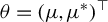
$\theta =(\mu ,\mu ^*)^{\top }$
 ,
$\Theta \subseteq \mathbb {R}^2$
 ,
$m(\theta )=\mu $
 , and
$U(\theta )=\mu ^*$
 .
Since the target population and the population from which data (2.7) are collected can be
different, partial identification naturally arises. We assume that the
identifiable and true treatment effects are constrained by
$\left \vert \mu ^*-\mu \right \vert \leq k$
 for some known
$k \geq 0$
 , implying

The planner must choose a statistical decision rule
$d\in \mathcal {D}_1:\mathbb {R}\rightarrow [0,1]$
 that maps observed data
$\hat {\mu }$
 to an action
$a\in [0,1]$
 . Taking (2.7) as an approximation, this stylized example could
reflect model uncertainty (e.g., a treatment effect is estimated in a
possibly somewhat misspecified model), external validity concerns (e.g.,
a randomized clinical trial was performed on volunteers), or a shift in
the environment (e.g., we transfer estimates from study populations to
treatment populations with slightly different covariates or are
concerned about distributional drift over time).
Example 2 (Ishihara and Kitagawa, Reference Ishihara and Kitagawa2021)
This example is taken from Ishihara and Kitagawa’s (Reference Ishihara and Kitagawa2021; see also Manski, Reference Manski2020) “evidence
aggregation” framework. A policy maker is interested in
implementing a new policy in country
$i=0$
 and observes estimates of the policy’s effect
for countries
$i=1,\ldots ,n$
 . Let
$Y=(Y_1,\ldots ,Y_n)^\top \in \mathbb {R}^n$
 denote these estimates and let
$(x_0,\ldots ,x_n)$
 be non-random, d-dimensional baseline
covariates. The policy maker is willing to extrapolate from her data by
assuming that the welfare contrast of interest equals
$U(\theta )=\theta (x_0)$
 and that

where
$\theta : \mathbb {R}^d \rightarrow \mathbb {R}$
 is an unknown Lipschitz function with known constant
C. For notational simplicity, we can further write
$\mu _i$
 for
$\theta (x_i)$
 . Thus,
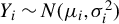
$Y_i \sim N(\mu _i,\sigma _i^2)$
 ,
$Y\sim N(\mu ,\Sigma )$
 , and
$U(\theta )=\mu _0$
 . The policy question is: Given data
Y, what proportion of the population in country
$i=0$
 should be assigned the new policy?
Let
$\left \Vert \beta \right \Vert :=\sqrt {\beta ^{\top }\beta }$
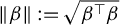 be the Euclidean norm of a vector
$\beta $
 . In this example, the identified set for the welfare
contrast
$\mu _0$
 is

The lower and upper bounds on
$I(\mu )$
 are simply intersection bounds:

2.3 Robust Bayes Optimality
Our setting up to here is as in Montiel Olea et al. (Reference Montiel Olea, Qiu and Stoye2026). We now connect it to the robust Bayes
literature by imposing a set of priors
$\Gamma $
 on
$\theta $
 . Following Giacomini and Kitagawa (Reference Giacomini and Kitagawa2021), we choose a particular single proper prior
$\pi _{\mu }$
 for
$\mu \in M$
 but leave the conditional prior of
$\theta $
 given
$\mu $
 , denoted as
$\pi _{\theta \mid \mu }$
 , unrestricted except for

Then, the class of priors
$\Gamma $
 consists of all priors on
$\theta $
 induced by the single prior
$\pi _{\mu }$
 and any conditional prior
$\pi _{\theta \mid \mu }$
 that meets (2.8). Intuitively, we choose a single prior on the point-identified
parameter and place no new restriction on the partially identified parameter
$U(\theta )$
 . One can pick any proper prior
$\pi _{\mu }$
 ; for tractability, we let
$\pi _{\mu }$
 be supported on two symmetric points
$\{\bar {\mu },-\bar {\mu }\}$
 with equal probability, where
$\bar {\mu }\in \mathbb {R}^n$
 is chosen by the decision maker. Henceforth,
$\Gamma $
 is understood to refer to the implied set of priors:

While the set of priors
$\Gamma $
 broadly puts us into “robust Bayes” territory,
it still does not pin down a uniquely best decision rule because the sign of
$U(\theta )$
 can remain ambiguous. Let

be the regret of action
$a\in [0,1]$
 . We evaluate decision rules d by their
expected regret, defined as

where for any
$x\in \mathbb {R}^n$
 ,
$\mathbb {E}_{x}[\cdot ]$
 denotes expectation taken over
$Y\sim N(x,\Sigma )$
 .
Even for given set of priors
$\Gamma $
 and commitment to expected regret, the Robust Bayes literature
contains multiple decision criteria that do not in general agree. The difference
lies in when (and how) the expectations regarding the unknown parameter
$\theta \in \Theta $
 are taken. For decision rule
$d\in \mathcal {D}_n$
 , let

be its Bayes expected regret under a prior
$\pi \in \Gamma $
 . Following Berger (Reference Berger1985,
Def. 12, p. 216), we introduce the first robust Bayes optimality
notion.
Definition 1 (
Ex-Ante
$\ \Gamma $
-Minimax Regret)

A decision rule
$d^* \in \mathcal {D}_n$
 is
$\Gamma $
 -minimax regret (henceforth
$\Gamma $
 -MMR) optimal if

An alternative “posterior” robustness notion is also common in
Bayesian analysis. For each action
$a\in [0,1]$
 , define posterior expected regret under prior
$\pi $
 (Berger, Reference Berger1985, Def. 8,
p. 159)

where
$\pi _{\theta \mid Y}$
 is the posterior distribution of
$\theta $
 given prior
$\pi $
 and data Y.Footnote
6
Then we have the following alternative optimality criterion (Berger,
Reference Berger1985, Def. 10, p. 205).
Definition 2 (Ex-Post
$\ \Gamma $
-Posterior Expected Regret)

A decision rule
$d^* \in \mathcal {D}_n$
 is
$\Gamma $
 -posterior expected regret (henceforth
$\Gamma $
 -PER) optimal if

If the decision maker’s action space is restricted to
$\{0,1\}$
 , that is, randomization is not allowed, the above definitions
are revised by replacing
$[0,1]$
 with
$\{0,1\}$
 .
The labeling of
$\Gamma $
 -MMR as “ex-ante” versus
$\Gamma $
 -PER as “ex-post” can be related to the timing of
a fictitious game against an adversarial Nature (see Section 3.3 for additional discussion). If
$\Gamma $
 were a singleton, the criteria would coincide and would also
agree with (single-prior) Bayes optimality. They do not in general agree
otherwise. The term “Gamma minimax” usually (and even
“robust Bayes” more often than not) refers to
$\Gamma $
 -MMR (e.g., see Berger, Reference Berger1985, Sect. 4.7.6).Footnote
7
While it is not our agenda to advocate for either criterion, some possible
considerations are as follows. The ex-ante approach may be perceived as more
suitable if the planner has commitment power and has also been justified
axiomatically (Hayashi, Reference Hayashi2008; Stoye,
Reference Stoye2011). We also find some numerical
and theoretical evidence that the
$\Gamma $
 -MMR rule may have desirable frequentist
properties, for example, in states of the world off the
prior’s support (see discussions at the end of Section 3.2). Regarding computational feasibility,
the ex-post approach is often easier due to the applicability of backward
induction and is routinely employed to quantify posterior robustness of
statistical decisions. On the other hand, recent work on numerical discovery of
minimax rules (Aradillas Fernández et al., Reference Aradillas Fernández, Blanchet, Olea, Qiu, Stoye and Tan2025; Guggenberger and Huang, Reference Guggenberger and Huang2025) may render the ex-ante approach more scalable. See additional
discussions in Appendix E.
The two-point structure of
$\pi _\mu $
 in (2.9)
appears in several related treatment choice problems with minimax regret
optimality criteria. For example, the least favorable prior (LFP) takes such a
form in a completely unconstrained minimax regret problem with point identified
(Stoye, Reference Stoye2009) or partially identified
(Stoye, Reference Stoye2012a; Yata, Reference Yata2021; Montiel Olea et al., Reference Montiel Olea, Qiu and Stoye2026) welfare contrast. In analogously constrained
minimax regret problems in which we restrict
$\mu \in [-\left |\bar {\mu }\right |,\left |\bar {\mu }\right |]$
 , extending the analyses in the preceding literature would also
imply a similar two-point symmetric structure for the LFP. Given these
precedents, we think our choice of
$\pi _\mu $
 represents a general feature of this class of minimax regret
decisions, in addition to offering computational tractability.
3 MAIN RESULTS
In this section, we solve for the two versions of robust Bayes optimality under the set of priors (2.9). Following Yata (Reference Yata2021), we invoke the following assumption.
Assumption 1.
-
(i) $\Theta $
is convex, centrosymmetric (i.e.,
$\theta \in \Theta $
implies
$-\theta \in \Theta $
) and nonempty. -
(ii) $m(\cdot )$
and
$U(\cdot )$
are linear.


These conditions are restrictive but encompass many examples of empirical relevance (see this article’s introduction, Montiel Olea et al., Reference Montiel Olea, Qiu and Stoye2026, and Yata, Reference Yata2021). Exploiting symmetry of the setting, we also set

This is a normalization because, by Lemma D.1, Assumption 1 implies
$\overline {I}(-\bar {\mu })+\underline {I}(-\bar {\mu })=-(\underline {I}(\bar {\mu })+\overline {I}(\bar {\mu }))$
 and we could always replace
$m(\cdot )\mapsto -m(\cdot )$
 ; furthermore, the case of
$\overline {I}(\bar {\mu })+\underline {I}(\bar {\mu })=0$
 gives rise to trivial solutions.Footnote
8
We say that a rule is a linear-index threshold rule if it has the
form
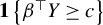
$\mathbf {1}\left \{ \beta ^{\top }Y\geq c\right \} $
 for some
$\beta \in \mathbb {R}^{n}$
 and
$c\in \mathbb {R}$
 . Linear-index threshold rules are non-randomized. They are of
particular interest because they form a complete class when
$U(\theta )$
 is point-identified (Karlin and Rubin, Reference Karlin and Rubin1956) and have received particular attention in the
recent literature (Ishihara and Kitagawa, Reference Ishihara and Kitagawa2021; Montiel
Olea et al., Reference Montiel Olea, Qiu and Stoye2026). For
both
$\Gamma $
 -MMR and
$\Gamma $
 -PER, we will clarify when linear-index threshold rules are optimal
and when they are not. For reasons that will become obvious, the following
linear-index threshold rule is of particular interest:

For each vector
$\beta \in \mathbb {R}^n$
 , let
$\left \Vert \beta \right \Vert {}_{\Sigma }:=\sqrt {\beta ^{\top }\Sigma \beta }$
 . Thus,
$\lVert w \lVert _{\Sigma } =\sqrt {w^{\top }\Sigma w}=\sqrt {\bar {\mu }^{\top }\Sigma ^{-1}\bar {\mu }}$
 . Denote by
$\Phi (\cdot )$
 the standard normal cdf and by
$\Phi ^{-1}(\cdot )$
 its inverse, that is, the corresponding quantile function.
3.1 Ex-Ante Robust Bayes Optimality
Theorem 1 (
$\Gamma $
-MMR Optimal Decisions)

Consider a treatment choice problem with welfare function (2.1), statistical model (2.3), and set of priors (2.9), that satisfy Assumption 1.
-
(i) If
(3.2) $$ \begin{align} \frac{\overline{I}(\bar{\mu})}{\overline{I}(\bar{\mu})-\underline{I}(\bar{\mu})}\geq\Phi(\lVert w \lVert_{\Sigma} ), \end{align} $$
then $d_{w,0}^{*}$
is uniquely
$\Gamma $
-MMR optimal. -
(ii) If
(3.3) $$ \begin{align} \frac{\overline{I}(\bar{\mu})}{\overline{I}(\bar{\mu})-\underline{I}(\bar{\mu})}<\Phi(\lVert w \lVert_{\Sigma} ), \end{align} $$
then a rule $d\in \mathcal {D}_{n}$
attains
$\Gamma $
-MMR if, and only if, it implies
(3.4) $$ \begin{align} \mathbb{E}_{-\bar{\mu}}[d^{*}(Y)] & = \frac{-\underline{I}(\bar{\mu})}{\overline{I}(\bar{\mu})-\underline{I}(\bar{\mu})}, \end{align} $$
(3.5) $$ \begin{align} \mathbb{E}_{\bar{\mu}}[d^{*}(Y)] & = \frac{\overline{I}(\bar{\mu})}{\overline{I}(\bar{\mu})-\underline{I}(\bar{\mu})}. \end{align} $$
In particular, any rule of the form $\mathbf {1}\left \{ w^{\top }Y\geq c\right \}$
for some
$c\in \mathbb {R}$
is not
$\Gamma $
-MMR optimal. The following rules, and any
convex combination of them, are
$\Gamma $
-MMR optimal: (3.6) $$ \begin{align} d^*_{\text{RT}}&:=\Phi\left(\frac{w^{\top}Y}{\tilde{\sigma}}\right), \end{align} $$
(3.7) $$ \begin{align} d^*_{\text{linear}}&:=\begin{cases} 0, & w^{\top}Y<-\rho^{*},\\ \frac{w^{\top}Y+\rho^{*}}{2\rho^{*}}, & -\rho^{*}\leq w^{\top}Y\leq\rho^{*},\\ 1, & w^{\top}Y>\rho^{*}, \end{cases} \end{align} $$
(3.8) $$ \begin{align} d^*_{\text{step}}&:=\begin{cases} \frac{1}{2} - \beta^*, & w^{\top}Y<0,\\ \frac{1}{2} + \beta^*, & w^{\top}Y\geq0,\\ \end{cases} \end{align} $$
where
$$\begin{align*}\tilde{\sigma}=\sqrt{\left[\frac{\lVert w \lVert_{\Sigma} ^{2}}{\Phi^{-1}\left(\frac{\overline{I}(\bar{\mu})}{\overline{I}(\bar{\mu})-\underline{I}(\bar{\mu})}\right)}\right]^{2}-\lVert w \lVert_{\Sigma} ^{2}},\end{align*}$$
$\rho ^{*}>0$
is unique and solves
$\int _{0}^{1}\Phi \left (\frac {2\rho ^{*}x-\rho ^{*}-\lVert w \lVert _{\Sigma } ^{2}}{\lVert w \lVert _{\Sigma } }\right )dx=\frac {-\underline {I}(\bar {\mu })}{\overline {I}(\bar {\mu })-\underline {I}(\bar {\mu })}$
, and $$\begin{align*}\beta^{*}=\frac{\frac{\overline{I}(\bar{\mu})}{\overline{I}(\bar{\mu})-\underline{I}(\bar{\mu})}-\frac{1}{2}}{2\Phi\left(\lVert w \lVert_{\Sigma} \right)-1}\in\left(0,\frac{1}{2}\right). \end{align*}$$
-
(iii) In case (3.3), among linear-index threshold rules of the form $\mathbf {1}\left \{ w^{\top }Y\geq c\right \}$
, the optimal thresholds are
$\pm c^{*}$
, where $$\begin{align*}c^{*}:=\lVert w \lVert_{\Sigma} ^2-\lVert w \lVert_{\Sigma} \Phi^{-1}\left(\frac{\overline{I}(\bar{\mu})}{\overline{I}(\bar{\mu})-\underline{I}(\bar{\mu})}\right)>0. \end{align*}$$
-
(iv) In case (3.3) and if $n>1$
, the following linear-index threshold rule
is also
$\Gamma $
-MMR optimal: $$\begin{align*}d_{w_{t^*},0}^{*}(Y):=\mathbf{1}\left\{ w_{t^*}^{\top}Y\geq0\right\} , \end{align*}$$
where $w_{t^*}=\Sigma ^{-1}\left (t^*\bar {\mu }+(1-t^*)\dot {\mu }\right )$
,
$\dot {\mu }\neq 0$
is such that
$\dot {\mu }^{\top }\Sigma ^{-1}\bar {\mu }=0$
, (3.9) $$ \begin{align} t^*:=\frac{1}{1\pm\sqrt{\frac{(1-s^{*})}{s^{*}}\frac{\lVert w \lVert_{\Sigma} ^{2}}{\lVert \Sigma^{-1} \dot{\mu}\lVert_{\Sigma} ^{2}}}}, \end{align} $$
and
$$\begin{align*}s^{*}:=\frac{\left[\Phi^{-1}\left(\frac{\overline{I}(\bar{\mu})}{\overline{I}(\bar{\mu})-\underline{I}(\bar{\mu})}\right)\right]^{2}}{\lVert w \lVert_{\Sigma} ^{2}}\in(0,1). \end{align*}$$
Thus, $d_{w_{t^*},0}^{*}$
is also optimal among all linear threshold
rules.


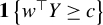




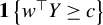







Theorem 1
reveals that the
$\Gamma $
 -MMR rules qualitatively change depending on whether condition
(3.2) is met or not. This
condition admits an intuitive interpretation: Up to clamping to the unit
interval (i.e., values outside this interval are mapped to its edges), the
left-hand side of (3.2) equals
the unique minimax regret optimal rule for known
$\mu $
 (Manski, Reference Manski2007b);
therefore, it arguably measures the model’s identification strength. The
right-hand side of (3.2) can be
interpreted as the informativeness of the data about which of
$\{-\bar {\mu },\bar {\mu }\}$
 obtained. Therefore, Theorem 1 says that if the model’s identification power
is sufficiently large compared to the informativeness of the data, then, the
unique
$\Gamma $
 -MMR optimal rule is
$d_{w,0}^{*}$
 , a non-randomized linear index rule with threshold
$0$
 that effectively ignores the partial identification issue. In
contrast, if the model’s identification power is small compared to the
informativeness of data, there are infinitely many
$\Gamma $
 -MMR optimal rules, all of which satisfy (3.4) and (3.5). Examples include suitably smoothed
versions of
$d_{w,0}^{*}$
 like
$d_{\text {RT}}^{*}$
 and
$d_{\text {linear}}^{*}$
 (the functional forms of which showed up in Montiel Olea et
al., Reference Montiel Olea, Qiu and Stoye2026) as well as
$d_{\text {step}}^{*}$
 (which is a new result).
To understand how these two “regimes” arise, it is helpful to think
of a zero-sum game against an adversarial Nature in which an MMR decision rule
and a distribution over parameter values (the LFP) form a Nash equilibrium.Footnote
9
If identification is strong in the sense of (3.2), this game has an
informative equilibrium: the LFP evenly randomizes over two
points
$(\mu ,U(\theta )) \in \{(\bar {\mu },\overline {I}(\bar {\mu })),(-\bar {\mu },\underline {I}(-\bar {\mu }))\}$
 , to which the unique Bayes response (and, therefore, uniquely
optimal MMR rule) is
$d_{w,0}^*$
 . In all other cases, the equilibrium is
uninformative: the LFP is supported on four points
$(\mu , U(\theta ))\in \{(\bar {\mu },\overline {I}(\bar {\mu })),(\bar {\mu },\underline {I}(\bar {\mu })),(-\bar {\mu },\overline {I}(-\bar {\mu })),(-\bar {\mu },\underline {I}(-\bar {\mu }))\}$
 with a probability profile such that the posterior expectation
of
$U(\theta )$
 always equals
$0$
 . While any decision rule best responds to this prior, not
every decision rule is MMR because the LFP must also best respond to the
decision rule. In this very structured setting, the latter is guaranteed by
conditions (3.4) and (3.5), establishing claim (ii) and
nonuniqueness of optimal decision rules. Indeed, even the non-randomized
threshold rules from Theorem 1(iv) do not reflect any updating along the game’s
equilibrium path; they rather use uninformative features of the data as
randomization device.
In the uninformative equilibrium, we encounter several additional findings.
First, despite the problem’s apparent symmetry,
$d_{w,0}^*$
 is not optimal even among linear-index
threshold rules that use the index
$w^{\top }Y$
 . Instead, Theorem 1(iii) characterizes exactly two optimal thresholds,
one positive and one negative. Second, while the particular linear-index
threshold rule
$d_{w,0}^*$
 is not
$\Gamma $
 -MMR optimal, in higher-dimensional problems (
$n>1$
 ), there do exist linear-index threshold rules that are. This
finding is in stark contrast to Montiel Olea et al. (Reference Montiel Olea, Qiu and Stoye2026), who find that, in a large class of special
cases, no linear index threshold rule is MMR optimal. The
crucial difference in settings is that the set of priors much constrains the
decision theoretic problem’s state space; as a result, the signal space
is much richer than the state space, and this can be exploited to mimic
randomization without nominally randomizing. Compare Manski’s (Reference Manski2025) abstract observation that, if a
policy maker is not allowed to explicitly randomize, sampling uncertainty can be
beneficial by providing an implicit randomization device. We note that this
phenomenon is reminiscent of classic “purification” results in
game theory (Dvoretzky, Wald, and Wolfowitz, Reference Dvoretzky, Wald and Wolfowitz1951; Khan, Rath, and Sun, Reference Khan, Rath and Sun2006).Footnote
10
In contrast, it is not deeply related to the general intuition that
“Bayesians don’t randomize.”
We next apply Theorem 1 to Example 1 and immediately get the following results.
Corollary 1 (
$\Gamma $
-MMR Decisions in Example 1)

In Example 1, the following statements are true:
-
(i) If
(3.10) $$ \begin{align} \frac{\bar{\mu}+k}{2k}\geq\Phi\left(\bar{\mu}/\sigma\right), \end{align} $$
then
$$\begin{align*}d_0^*(\cdot):=\mathbf{1}\{\hat{\mu}\geq0\} \end{align*}$$is the unique $\Gamma $
-MMR optimal decision rule.
-
(ii) If (3.10) fails, then a rule $d \in \mathcal {D}_1$
attains
$\Gamma $
-MMR if, and only if, it implies
(3.11) $$ \begin{align} \mathbb{E}[d(\hat{\mu}) \mid \mu=-\bar{\mu}] &= \frac{-\bar{\mu}+k}{2k}, \end{align} $$
(3.12) $$ \begin{align} \mathbb{E}[d(\hat{\mu}) \mid \mu=\bar{\mu}] &= \frac{\bar{\mu}+k}{2k}. \end{align} $$
In particular, no linear threshold rule is $\Gamma $
-MMR optimal. The following rules, and any
convex combination of them, are all
$\Gamma $
-MMR optimal: (3.13) $$ \begin{align} d^*_{\text{RT}}&:=\Phi\left(\frac{\hat{\mu}}{\tilde{\sigma}}\right), \end{align} $$
(3.14) $$ \begin{align} d^*_{\text{linear}}&:=\begin{cases} 0, &\hat{\mu}<-\frac{\sigma^{2}\rho^{*}}{\bar{\mu}},\\ \frac{\bar{\mu}\hat{\mu}+\sigma^{2}\rho^{*}}{2\sigma^{2}\rho^{*}}, & -\frac{\sigma^{2}\rho^{*}}{\bar{\mu}}\leq \hat{\mu}\leq\frac{\sigma^{2}\rho^{*}}{\bar{\mu}},\\ 1, & \hat{\mu}>\frac{\sigma^{2}\rho^{*}}{\bar{\mu}}, \end{cases} \end{align} $$
(3.15) $$ \begin{align} d^*_{\text{step}}&:=\begin{cases} \frac{1}{2} - \frac{\bar{\mu}}{2k\left(2\Phi\left(\frac{\bar{\mu}}{\sigma}\right)-1\right)}, & \hat{\mu}<0,\\ \frac{1}{2} + \frac{\bar{\mu}}{2k\left(2\Phi\left(\frac{\bar{\mu}}{\sigma}\right)-1\right)}, & \hat{\mu}\geq0,\\ \end{cases} \end{align} $$
where
$$\begin{align*}\tilde{\sigma}=\sigma\sqrt{\left[\frac{\bar{\mu}}{\sigma \Phi^{-1}\left(\frac{\bar{\mu}+k}{2k}\right)}\right]^{2}-1 },\end{align*}$$
and $\rho ^{*}>0$
is unique and solves
$\int _{0}^{1}\Phi \left (\frac {2\rho ^{*}x-\rho ^{*}-({\unicode{x2044}} {\bar {\mu }}{\sigma }) ^{2}}{{\unicode{x2044}} {\bar {\mu }}{\sigma } }\right )dx=\frac {-\bar {\mu }+k}{2k}$
. -
(iii) In case (ii), the best linear threshold rules in terms of $\Gamma $
-minimax regret are
$\mathbf {1}\{\hat {\mu }\geq \pm c^*\}$
, where $$ \begin{align*} c^* = \bar{\mu} - \sigma \Phi^{-1}\left(\frac{\bar{\mu}+k}{2k}\right). \end{align*} $$





Note that there is no analog to Theorem 1’s case (iv); indeed, no linear threshold rule
is optimal in case (ii). This is because the scalar nature of the signal
Y shuts down the aforementioned purification mechanism. See
Figure 1 for an illustration
of different
$\Gamma $
 -MMR optimal rules in Example 1 for selected parameter values of
$k,\sigma $
 , and
$\bar {\mu }$
 .
$\Gamma $
 -MMR optimal rules in Example 1.
Note: This figure reports the
$\Gamma $
 -MMR optimal rules in Example 1 for various
combinations of parameter values. In the top two panels, the
combinations of parameter values satisfy (3.10). Therefore, the unique
$\Gamma $
 -MMR optimal rule is
$d^*_0$
 . In the bottom two panels, (3.10) fails. As a result,
$d^*_0$
 is no longer
$\Gamma $
 -MMR optimal. Instead,
$d^*_{\text {RT}}$
 ,
$d^*_{\text {linear}}$
 , and
$d^*_{\text {step}}$
 are all
$\Gamma $
 -MMR optimal.

Figure 1 Long description
A four-panel grid of line graphs. Each graph has an x-axis labeled mu-hat ranging from minus 3 to 3 and a y-axis labeled d dot ranging from 0.0 to 1.0. A legend at the bottom identifies four rules: d super star sub 0 (dashed teal), d super star sub R T (solid dark red), d super star sub linear (dashed green), and d super star sub step (dash-dot grey).
* Top-left panel (k equals 1, sigma equals 1, mu bar equals 1.5): Shows only the d super star sub 0 rule, which is a step function that is 0 for mu-hat less than 0 and 1 for mu-hat greater than 0.
* Top-right panel (k equals 1, sigma equals 1, mu bar equals 0.5): Identical to the top-left, showing only the d super star sub 0 step function.
* Bottom-left panel (k equals 1, sigma equals 0.5, mu bar equals 0.5): Displays multiple overlapping rules. d super star sub R T follows a steep S-shaped logistic curve. d super star sub linear follows a steep linear diagonal through the origin before leveling off. d super star sub step is a three-level step function starting at approximately 0.13, jumping to 0.5 at mu-hat equals 0, and jumping to 0.87 for mu-hat greater than 0.
* Bottom-right panel (k equals 2, sigma equals 1, mu bar equals 0.5): Similar to the bottom-left but with shallower slopes. d super star sub R T is a gradual S-curve. d super star sub linear is a gradual diagonal. d super star sub step has three levels at approximately 0.17, 0.5, and 0.83.
3.2 Ex-Post Robust Bayes Optimality
Theorem 2 (
$\Gamma $
-PER Optimal Decisions)

Suppose all conditions in Theorem 1 hold true. Then:
-
(i) If $\underline {I}(\bar {\mu })<0<\overline {I}(\bar {\mu })$
, the unique
$\Gamma $
-PER optimal rule is $$\begin{align*}d_{\mathrm{PER}}^{*}(Y)=\begin{cases} \frac{-\underline{I}(\bar{\mu})}{\overline{I}(\bar{\mu})-\underline{I}(\bar{\mu})}, & \text{if }w^{\top}Y<0, \\ \frac{\overline{I}(\bar{\mu})}{\overline{I}(\bar{\mu})-\underline{I}(\bar{\mu})}, & \text{if }w^{\top}Y\geq0. \end{cases} \end{align*}$$
Otherwise, $d_{w,0}^{*}$
is
$\Gamma $
-PER optimal. -
(ii) $d_{w,0}^{*}$
is always the
$\Gamma $
-PER optimal non-randomized rule.



The results of Theorem 2 offer some important clarifications regarding
$\Gamma $
 -PER in treatment choice problems with partial identification.
First, even if regret is evaluated according to the posterior distribution, it
is not necessarily true that optimal rules are non-randomized. In fact, whenever
there is model ambiguity regarding the sign of
$U(\theta )$
 (i.e.,
$\underline {I}(\bar {\mu })<0<\overline {I}(\bar {\mu })$
 ), the unique
$\Gamma $
 -PER optimal rule is randomized. Therefore, restricting the
action space to
$\{0,1\}$
 in such problems is not without loss of
generality even under the
$\Gamma $
 -PER criterion. Comparing results with Theorem 1 also allows for instructive
observations on when
$\Gamma $
 -PER and
$\Gamma $
 -MMR optimal rules agree or disagree; we elaborate these in
Corollary 3.
Applying Theorem 2 to
Example 1, we
finally obtain the following corollary.
Corollary 2
$(\Gamma $
-PER Rules in Example 1)

In Example 1, the following statements are true:
-
(i) If $\bar {\mu }<k$
, then
$\Gamma $
-PER is uniquely minimized by $$\begin{align*}d^*_{\mathrm{PER}}(\hat{\mu}) = \begin{cases} \frac{k + \bar{\mu}}{2k} & \text{if } \hat{\mu} \geq 0\\ \frac{k-\bar{\mu}}{2k} & \text{if } \hat{\mu} < 0. \end{cases}\end{align*}$$
-
(ii) If $\bar {\mu }\geq k$
, then
$d_0^*$
is
$\Gamma $
-PER optimal. Furthermore, it is always the
$\Gamma $
-PER optimal threshold rule.


In Figure 2, we depict
$\Gamma $
 -PER optimal rules for Example 1 with the same parameter values
considered in Figure 1. We see
clearly that
$\Gamma $
 -MMR and -PER optimal rules coincide (if randomization is
allowed) only in the special case when
$k\leq \bar {\mu }$
 , an observation we generalize in Corollary 3. More specifically, in the
top left panel of Figure 2, as
$k\leq \bar {\mu }$
 ,
$\Gamma $
 -MMR and -PER coincide and are the non-randomized threshold
rule
$d^*_{0}$
 . In the top right panel,
$k>\bar {\mu }$
 and the
$\Gamma $
 -PER optimal rule becomes
$d^*_{\text {PER}}$
 . However, since (3.10) still holds,
$d^*_0$
 is still
$\Gamma $
 -MMR optimal. For the bottom two panels, as it still holds
$k>\bar {\mu }$
 ,
$d^*_{\text {PER}}$
 is still
$\Gamma $
 -PER optimal. However, the associated parameter values imply
that (3.10) fails. As a result,
$d^*_{0}$
 is no longer
$\Gamma $
 -MMR optimal and many
$\Gamma $
 -MMR rules exist. But even in these cases,
$\Gamma $
 -MMR and -PER rules differ, as among the class of step function
rules (which contain
$d^*_{\text {PER}}$
 ), only
$d^*_{\text {step}}$
 is
$\Gamma $
 -MMR optimal, still different from
$d^*_{\text {PER}}$
 .
$\Gamma $
 -PER optimal rules in Example 1.
Note: This figure reports the
$\Gamma $
 -PER optimal rules for the same parameter values
considered in Figure 1. In the top left panel,
$\Gamma $
 -PER and
$\Gamma $
 -MMR optimal rules coincide and are both
$d^*_{0}$
 . For the rest of the panels, the unique
$\Gamma $
 -PER optimal rules are all
$d^*_{\text {PER}}$
 and are different from any
$\Gamma $
 -MMR optimal rules.
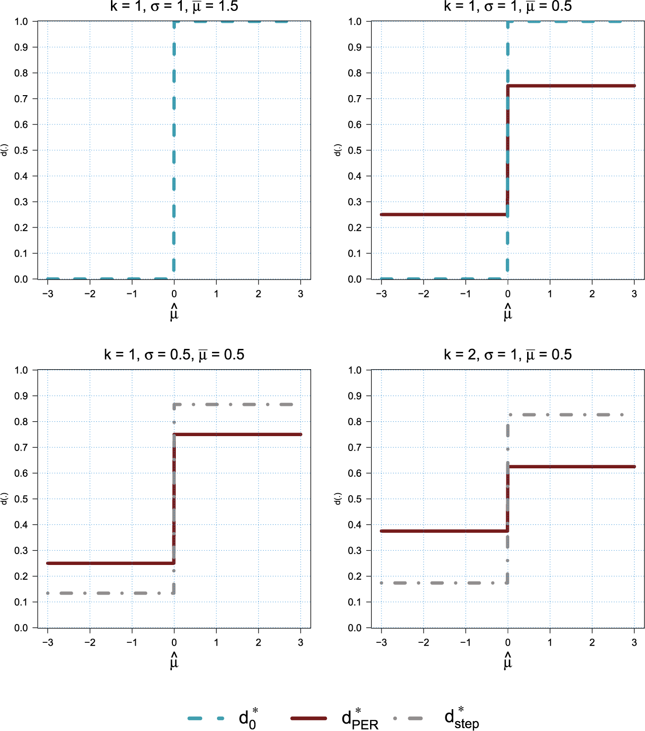
Figure 2 Long description
Each of the four panels shares a common X-axis labeled mu-hat ranging from minus 3 to 3 and a Y-axis labeled d dot open parenthesis dot close parenthesis ranging from 0.0 to 1.0. A legend at the bottom identifies three rules: d sub 0 super star (dashed teal line), d sub P E R super star (solid maroon line), and d sub step super star (dash-dotted grey line).
* Top-left panel (k = 1, sigma = 1, mu bar = 1.5): The dashed teal line d sub 0 super star is at 0 for mu-hat less than 0 and jumps to 1 for mu-hat greater than 0. The maroon line is identical and hidden behind it.
* Top-right panel (k = 1, sigma = 1, mu bar = 0.5): The dashed teal line remains a step from 0 to 1 at mu-hat equals 0. The solid maroon line d sub P E R super star shows a smaller step, starting at 0.25 and jumping to 0.75 at mu-hat equals 0.
* Bottom-left panel (k = 1, sigma = 0.5, mu bar = 0.5): The solid maroon line is at 0.25 for mu-hat less than 0 and 0.75 for mu-hat greater than 0. The dash-dotted grey line d sub step super star shows a wider step, from approximately 0.15 to 0.85.
* Bottom-right panel (k = 2, sigma = 1, mu bar = 0.5): The solid maroon line is at approximately 0.38 for mu-hat less than 0 and 0.62 for mu-hat greater than 0. The dash-dotted grey line shows a step from approximately 0.18 to 0.82.
Applying Montiel Olea et al. (Reference Montiel Olea, Qiu and Stoye2026, Thm.
1) to the current setting, we can conclude that all rules, including both
$\Gamma $
 -MMR and
$\Gamma $
 -PER optimal rules, are at least admissible. Moreover, by
definition, the
$\Gamma $
 -MMR rule will have the lower value of the (ex ante) game.
Therefore, it might be more useful to compare the (frequentist) profiled regrets
(Montiel Olea et al., Reference Montiel Olea, Qiu and Stoye2026) of ex-post
$\Gamma $
 -PER and other rules as a function of the true but unknown mean
$\mu $
 of data
$\hat {\mu }$
 . In the context of Example 1, we can report
$\bar {R}(d,\mu ):=\sup _{\mu ^*\in [\mu -k,\mu +k]}R(d,\mu ,\mu ^*)$
 as
$\mu $
 varies for each rule d, where
$R(d,\mu ,\mu ^*)$
 is the expected regret of rule d as a
function of
$\mu $
 and
$\mu ^{*}$
 . We report several findings (we emphasize that these are not
obvious: we took an ex-ante perspective but did not restrict ourselves to those
values of
$\mu $
 that the prior allows). First, in both panels of
Figure 3, the profiled
expected regret of the
$\Gamma $
 -PER rule exceeds that of the
$\Gamma $
 -MMR rule. Therefore, in this particular example,
$\Gamma $
 -MMR arguably outperforms
$\Gamma $
 -PER from a broader frequentist point of view. Second, we in
fact prove that, whenever
$\bar {\mu }$
 is sufficiently small and k is sufficiently
large, the
$\Gamma $
 -PER rule is profiled-regret dominated, that is, there exists a
rule
$d\neq d^*_{\text {PER}}$
 such that

for all
$\mu \in \mathbb {R}$
 with the inequality strict for some
$\mu $
 (see Lemma D.2 in Appendix D
for an exact statement). Intuitively, the
$\Gamma $
 -PER rule mixes between a coin flip rule and the naive
threshold rule (
$d_0^{*}$
 ). When
$\bar {\mu }$
 is small,
$\Gamma $
 -PER rule is more analogous to the coin flip rule, which
Montiel Olea et al. (Reference Montiel Olea, Qiu and Stoye2026) show to be
dominated in terms of profiled regret; also, its profiled regret fails to vanish
as
$\mu \to \pm \infty $
 even though the optimal treatment is known ex ante in this
case. Furthermore, Figure 3
reveals that the
$\Gamma $
 -MMR rule
$d^{*}_{\text {linear}}$
 , though not globally MMR optimal, in some cases has
essentially the same profiled risk function as the least randomizing global MMR
optimal rule (Montiel Olea et al., Reference Montiel Olea, Qiu and Stoye2026).
This may lend a Robust Bayes interpretation to the latter.
Profiled regret of
$\Gamma $
 -PER and other rules in Example 1.
Note: This figure reports the (frequentist)
profiled regrets, as a function of the true mean
$\mu $
 of data
$\hat {\mu }$
 , of
$\Gamma $
 -PER rule,
$\Gamma $
 -MMR linear rule, and the least randomizing global
MMR optimal rule (Montiel Olea et al., Reference Montiel Olea, Qiu and Stoye2026) for the parameter values considered
in Montiel Olea et al. (Reference Montiel Olea, Qiu and Stoye2026,
Fig. 2). In the left plot, we see that
$\Gamma $
 -PER rule is visually dominated. In both plots, the
profiled regret of
$\Gamma $
 -MMR linear rule and the least randomizing global
MMR optimal rule look very similar and are essentially overlapping
with each other.

Figure 3 Long description
A two-panel line graph. Both panels share a horizontal axis labeled mu ranging from minus 30 to 30 and a vertical axis labeled Profiled Regret ranging from 0 to 15.
* Left Plot (k = 18.6, sigma = 3.9, mu bar = 4.7): A solid dark red line representing d super star P E R forms a U-shaped curve that stays above the other rules, reaching a minimum of approximately 9 at mu equals 0. Two other lines, a grey dashed line for d super star linear global M M R and a teal dash-dot line for d super star linear ex-ante Gamma M M R, are perfectly overlapped. They form a bell-shaped curve peaking at approximately 9 when mu is 0 and tapering to 0 as mu moves toward minus 30 or 30.
* Right Plot (k = 18.6, sigma = 3.9, mu bar = 14): The solid dark red line d super star P E R shows a more complex M-shaped profile in the center with two peaks near 11 and a local minimum at mu equals 0, then transitions into linear segments at the far left and right. The grey dashed and teal dash-dot lines remain overlapped, maintaining the same bell-shaped curve seen in the first plot, peaking at 9 when mu is 0.
A legend at the bottom identifies the three rules: d super star P E R (solid red), d super star linear (global M M R) (grey dashed), and d super star linear (ex-ante Gamma M M R) (teal dash-dot).
3.3 Ex-Ante and Ex-Post in the Game against Nature
The different approaches analyzed here can all be expressed as different timing assumptions in the statistical game. The distinction is quite obvious for ex-ante versus ex-post: In the former (and original Waldian) perspective, this game is simultaneous move; in particular, Nature moves before data Y are realized. In the ex-post perspective, Nature sees Y before choosing a prior. It is immediately clear that this may be easier to solve because it allows for backward induction. There is also an immediate sense that solutions might not agree, as we indeed found.
But whether the decision maker is allowed to (or at least wants to) randomize or
not can equally be thought of as changing the game’s timing, providing
another way to think about the action space for the ex-ante and
ex-post approaches. The more standard perspective is that the decision maker may
randomize over decision rules and Nature must move before learning the outcome
of this randomization. By the nature of zero-sum games, this setup will
frequently yield randomized solutions. In consequence, it is essential to define
the decision maker’s action space as
$[0,1]$
 . In contrast, if Nature is allowed to move after the decision
maker’s randomization is realized, then any incentive to randomize is
gone and we may as well restrict the action space to
$\{0,1\}$
 .
Theorems 1 and 2 clarify that these distinctions actually matter in an interesting example. We spell this out in Corollary 3, which considers both cases when randomization is allowed and not allowed. The bottom line is that the assessment is quite sensitive to how the problem is set up. If underlying parameters lead to sufficiently small identification power, the criteria disagree.
Corollary 3. Consider a treatment choice problem with welfare function (2.1) and statistical model (2.3) that satisfies Assumption 1.
-
(i) Suppose randomization is allowed. Then the $\Gamma $
-MMR and
$\Gamma $
-PER optimal rules coincide if, and only
if,
$\underline {I}(\bar {\mu })\geq 0$
. -
(ii) Suppose randomization is not allowed. Then the $\Gamma $
-MMR and
$\Gamma $
-PER optimal rules coincide if, and only
if, (3.17) $$ \begin{align} \frac{\overline{I}(\bar{\mu})}{\overline{I}(\bar{\mu})-\underline{I}(\bar{\mu})}\geq \Phi(\lVert w \lVert_{\Sigma} ). \end{align} $$


Thus, if randomization is allowed,
$\Gamma $
 -MMR and
$\Gamma $
 -PER optimal rules coincide only in the somewhat trivial case
in which we a
priori know that
$U(\theta )$
 and
$\mu $
 have the same sign, so that optimal treatment choice reduces
to Bayesian inference on the point identified
$\mu $
 . They disagree in all other cases, including in settings where
there are infinitely many
$\Gamma $
 -MMR optimal rules.
One might expect more agreement once randomization is excluded; after all, this
leads to a much simpler action space. Part (ii) shows that there is some truth
to this: The condition for agreement changes from
$\underline {I}(\bar {\mu })\geq 0$
 to the strictly weaker (3.17). However, the criteria continue to
disagree in many cases. It may be instructive to think of these cases in terms
of “comparative statics.” For example, consider holding all
parameters of the problem fixed but scaling the signal variance
$\Sigma $
 by a positive scalar, say to reflect a change in sample size.
Then (3.17) will hold if, and
only if,
$\Sigma $
 is large enough; hence, as long as
$\underline {I}(\bar {\mu })\geq 0$
 , increasing sample size will eventually cause disagreement
between
$\Gamma $
 -MMR and -PER even if randomization is excluded. Similarly, for
fixed
$\Sigma $
 ,
$\Gamma $
 -MMR and -PER rules will always disagree if the model’s
identification power is small enough.
4 CONCLUSION
We studied treatment choice problems that display partial identification through the
lens of the robust Bayes criteria. To do so, we take the general framework of Yata
(Reference Yata2021) and others and embed in it a
simple example of the set of priors advocated by Giacomini and Kitagawa (Reference Giacomini and Kitagawa2021). We describe and contrast (ex-ante)
$\Gamma $
 -minimax regret and (ex-post)
$\Gamma $
 -posterior expected regret and analytically derive optimal
solutions with and without randomization.
Our results contain two key messages that we think are valuable to the literature. First, with partial identification and multiple priors, ex-ante and ex-post assessments do not agree in general, whether or not randomized rules are allowed. This may at first seem expected due to dynamic inconsistency of multiple prior Bayes criteria, but was not obvious in view of the set of prior’s specific structure. Second, randomization can be optimal in both ex-ante and ex-post problems—it is with loss of generality to exclude them even when regret is evaluated ex-post. The contrast between the results also illustrates a need to better understand the comparative advantages—whether from a theoretical or practical perspective—of using one criterion over the other.
An obvious limitation lies in our use of a convenient but restrictive prior on
$\mu $
 . As we discovered in Section 3.2, the
$\Gamma $
 -MMR rule also performs well across other values of
$\mu $
 ; however, this may be related to the fact that the globally LFP in
this setting has a two-point structure on
$\mu $
 as well and would obviously not generalize to arbitrary uses of
restrictive priors. We provide some insight on more general priors in
Appendix E. In short, the
tractability advantage of
$\Gamma $
 -PER may become pronounced in such settings, although we hope that
recent computational developments (Aradillas Fernández et al., Reference Aradillas Fernández, Blanchet, Olea, Qiu, Stoye and Tan2025; Guggenberger and Huang, Reference Guggenberger and Huang2025) will attenuate this concern.
A PROOFS OF MAIN RESULTS
Proofs will frequently claim and verify equilibria of the fictitious game against Nature. Recall that, from basic facts about zero-sum games, if a decision rule uniquely best responds to some least favorable prior, it must be the unique equilibrium rule.
A.1 Proof of Theorem 1
A.1.1 Statement (i)
The expected regret of decision rule d is

Recall that, by the definition of
$\Gamma $
 , we have
$\pi _{\mu }\sim \text {unif}(\{-\bar {\mu },\bar {\mu }\})$
 and, given
$\mu =\pm \bar {\mu }$
 ,
$\pi _{\theta \mid \mu }(U(\theta )\in I(\mu ))=1$
 . Therefore, the Bayes expected regret of
d under prior
$\pi \in \Gamma $
 equals

where
$\mathbb {E}_{\bar {\mu }}[d]:=\mathbb {E}_{\bar {\mu }}[d(Y)]$
 and
$\mathbb {E}_{-\bar {\mu }}[d]:=\mathbb {E}_{-\bar {\mu }}[d(Y)]$
 . One can easily solve for

The least favorable prior
$\pi ^*$
 equals

Lemma B.1 shows that the unique Bayes rule against
$\pi ^*$
 is

Lemma B.2 establishes that
$\sup _{\pi \in \Gamma }r(d_{w,0}^{*},\pi )=r(d_{w,0}^{*},\pi ^{*})$
 as long as (3.2) holds true. This establishes the claim.
A.1.2 Statement (ii)
Step 1: We show that when (3.3) holds, any rule
$d\in \mathcal {D}_{n}$
 is
$\Gamma $
 -MMR optimal if

The least favorable prior
$\pi ^{*}$
 is such that
$\mu \sim \text {unif}(\{-\bar {\mu },\bar {\mu }\})$
 , and when
$\mu =\bar {\mu }$
 ,

where
$p_{1}>0$
 is such that
$p_{1}\overline {I}(\bar {\mu })+(1-p_{1})\underline {I}(\bar {\mu })=0$
 , and when
$\mu =-\bar {\mu }$
 ,

where
$p_{2}$
 is such that
$p_{2}\overline {I}(-\bar {\mu })+(1-p_{2})\underline {I}(-\bar {\mu })=0$
 . Lemma B.3 establishes that any decision rule is Bayes against this
prior (intuitively because the data are uninformative), and
Lemma B.4
further shows that, for any rule d that satisfies
(A.2),
$\sup _{\pi \in \Gamma }r(d,\pi )=r(d,\pi ^*)$
 obtains. This establishes the claim.
Step 2: We next verify the “only if”
statement. Recall that the least favorable prior
$\pi ^*$
 must best respond to any optimal decision rule, that
is, for any MMR optimal rule d,
$\pi ^*$
 must solve

This, however, requires that Nature is indifferent
between
$\overline {I}(\bar {\mu })$
 and
$\underline {I}(\bar {\mu })$
 when
$\mu =\bar {\mu }$
 and similarly between
$\overline {I}(-\bar {\mu })$
 and
$\underline {I}(-\bar {\mu })$
 when
$\mu =-\bar {\mu }$
 . That is, we must have

which is equivalent to (A.2).
Step 3: We show a rule of form
$\mathbf {1}\left \{ w^{\top }Y\geq c\right \} $
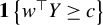 for some
$c\in \mathbb {R}$
 cannot be
$\Gamma $
 -MMR optimal when (3.3) holds. Note
$w=\Sigma ^{-1}\bar {\mu }$
 . Thus,

Suppose by contradiction that a rule
$\mathbf {1}\left \{ w^{\top }Y\geq c\right \} $
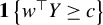 is optimal, then, by statement (ii), we have


By symmetry, (A.3) and (A.4) can both hold only if
$c=0$
 . But (3.3) then implies that

so that (A.3) cannot in fact hold when
$c=0$
 , a contradiction.
Step 4: We verify that
$d_{\text {RT}}^*$
 ,
$d_{\text {linear}}^*$
 , and
$d_{\text {step}}^*$
 are all
$\Gamma $
 -MMR optimal. Due to symmetry, it suffices to show that

To see
$\mathbb {E}_{\bar {\mu }}[d_{\text {RT}}^*]=\frac {\overline {I}(\bar {\mu })}{\overline {I}(\bar {\mu })-\underline {I}(\bar {\mu })}$
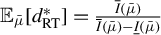 , consider the random threshold rule
$\mathbf {1}\left \{ w^\top Y\geq \xi \right \}$
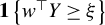 , where
$\xi \sim N(0,\tilde {\sigma }^{2})$
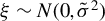 is independent of Y. As
$w^\top Y-\xi \sim N\left (\lVert w \lVert _{\Sigma } ^2,\lVert w \lVert _{\Sigma } ^2+\tilde {\sigma }^2\right )$
 , algebra shows

as required. To see
$\mathbb {E}_{\bar {\mu }}[d_{\text {linear}}^*]=\frac {\overline {I}(\bar {\mu })}{\overline {I}(\bar {\mu })-\underline {I}(\bar {\mu })}$
 , let
$\rho>0$
 and

Applying Lemma C.7 in Montiel Olea et al. (Reference Montiel Olea, Qiu and Stoye2026) and integration by parts yield

Note that
$\lim _{\rho \downarrow 0}f(\rho )=1-\Phi (-\lVert w \lVert _{\Sigma } ) = \Phi (\lVert w \lVert _{\Sigma } )>\frac {\overline {I}(\bar {\mu })}{\overline {I}(\bar {\mu })-\underline {I}(\bar {\mu })}$
 , while L’Hopital’s rule implies

where the last inequality follows from
$\overline {I}(\bar {\mu })+\underline {I}(\bar {\mu })>0$
 and
$1>\Phi \left (\lVert w \lVert _{\Sigma } \right )>\frac {\overline {I}(\bar {\mu })}{\overline {I}(\bar {\mu })-\underline {I}(\bar {\mu })}$
 . Furthermore, by applying the chain rule,
$\frac {\partial f(\rho )}{\partial \rho }<0$
 . Therefore,
$f(\cdotp )$
 is strictly decreasing in
$(0,\infty )$
 . We conclude that there must exist some unique
$\rho ^{*}>0$
 such that
$f(\rho ^{*})=\frac {\overline {I}(\bar {\mu })}{\overline {I}(\bar {\mu })-\underline {I}(\bar {\mu })}$
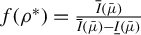 , or equivalently,
$\int _{0}^{1}\Phi \left (\frac {2\rho ^{*}x-\rho ^{*}-\lVert w \lVert _{\Sigma } ^{2}}{\lVert w \lVert _{\Sigma } }\right )dx=\frac {-\underline {I}(\bar {\mu })}{\overline {I}(\bar {\mu })-\underline {I}(\bar {\mu })}$
 , which implies
$\mathbb {E}_{\bar {\mu }}[d_{\text {linear}}^{*}]=\frac {\overline {I}(\bar {\mu })}{\overline {I}(\bar {\mu })-\underline {I}(\bar {\mu })}$
 .
Finally, we verify that
$\mathbb {E}_{\bar {\mu }}[d_{\text {step}}^{*}]=\frac {\overline {I}(\bar {\mu })}{\overline {I}(\bar {\mu })-\underline {I}(\bar {\mu })}$
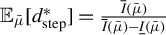 . For any
$\beta \in \left (0,\frac {1}{2}\right )$
 , consider the following step function rule:

One then has

Setting
$\mathbb {E}_{\bar {\mu }}[d_{\text {step},\beta ^{*}}]=\frac {\overline {I}(\bar {\mu })}{\overline {I}(\bar {\mu })-\underline {I}(\bar {\mu })}$
 yields
$\beta ^{*}=\frac {\frac {\overline {I}(\bar {\mu })}{\overline {I}(\bar {\mu })-\underline {I}(\bar {\mu })}-\frac {1}{2}}{2\Phi \left (\lVert w \lVert _{\Sigma } \right )-1}$
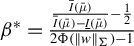 . As
$\overline {I}(\bar {\mu })+\underline {I}(\bar {\mu })>0$
 and (3.3) holds,
$\frac {\overline {I}(\bar {\mu })}{\overline {I}(\bar {\mu })-\underline {I}(\bar {\mu })}>\frac {1}{2}$
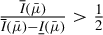 and therefore
$\beta ^{*}>0$
 . Furthermore,
$\beta ^{*}<\frac {1}{2}$
 holds due to (3.3) as well. Since
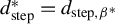
$d_{\text {step}}^{*}=d_{\text {step},\beta ^{*}}$
 , we conclude that
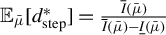
$\mathbb {E}_{\bar {\mu }}[d_{\text {step}}^{*}]=\frac {\overline {I}(\bar {\mu })}{\overline {I}(\bar {\mu })-\underline {I}(\bar {\mu })}$
 .
A.1.3 Statement (iii)
For any rule of form
$d_{w,c}(Y):=\mathbf {1}\{w^{\top }Y\geq c\}$
 , where
$w=\Sigma ^{-1}\bar {\mu }$
 and
$c\in \mathbb {R}$
 , we may calculate

and (due to Lemma D.1, recalling
$\lVert w \lVert _{\Sigma } ^{2}=w^{\top }\Sigma w=\bar {\mu }^{\top }\Sigma ^{-1}\bar {\mu }$
 )

Lemma B.5 shows that g is decreasing on
$[0,c^*]$
 and increasing on
$[c^{*},\infty )$
 , implying that the optimal threshold rule is
$d_{w,c^{*}}$
 when
$c\in [0,\infty )$
 . By symmetry,
$d_{w,-c^*}$
 is optimal when
$c\in (-\infty ,0]$
 , and
$d_{w,-c^*}$
 and
$d_{w,c^*}$
 share the same worst-case expected regret.
A.1.4 Statement (iv)
In case (3.3) and when
$n>1$
 , there exists
$\dot {\mu }\neq \mathbf {0}$
 such that
$\dot {\mu }^{\top }\Sigma ^{-1}\bar {\mu }=0$
 , that is,
$\dot {\mu }$
 is orthogonal to
$\Sigma ^{-1}\bar {\mu }$
 . For any
$t\in \mathbb {R}$
 , let

Lemma B.6 shows that when
$t=t^{*}$
 ,
$\mathbb {E}_{\bar {\mu }}[d_{w_{t^{*}},0}(Y)]=\frac {\overline {I}(\bar {\mu })}{\overline {I}(\bar {\mu })-\underline {I}(\bar {\mu })}$
 . By symmetry, one then also has
$\mathbb {E}_{-\bar {\mu }}[d_{w_{t^{*}},c}(Y)]=\frac {-\underline {I}(\bar {\mu })}{\overline {I}(\bar {\mu })-\underline {I}(\bar {\mu })}$
 . Applying statement (ii) yields that
$d_{w_{t^{*}},0}$
 is MMR optimal.
A.2 Proof of Corollary 1
In Example 1,
$\overline {I}(\bar {\mu })=\bar {\mu }+k,\ \underline {I}(\bar {\mu })=\bar {\mu }-k$
 ,
$\Sigma =\sigma ^{2}$
 . The results of the corollary follow directly from
Theorem 1(i)–(iii).
A.3 Proof of Theorem 2
Recall that the
$\Gamma $
 -PER optimal rule solves

where
$L(a,\theta )=U(\theta )(\mathbf {1}\{U(\theta )\geq 0\}-a)$
 and
$\pi _{\theta \mid Y}$
 is the posterior distribution of
$\theta $
 given Y. If randomization is not allowed,
the
$\Gamma $
 -PER optimal rule solves

Statement (i) then follows from Lemma C.1; statement (ii) follows from Lemma C.2.
A.5 Proof of Corollary 3
(i) “If”: If
$\underline {I}(\bar {\mu })\geq 0$
 , then Theorems 1(i) and 2(i) apply and establish that
$d_{w,0}^*$
 is both the unique
$\Gamma $
 -MMR and the unique
$\Gamma $
 -PER optimal rule.
“Only if”: If
$\underline {I}(\bar {\mu })<0$
 , then
$d_{\text {PER}}^{*}$
 is uniquely
$\Gamma $
 -PER optimal by Theorem 2(i). If condition (3.2) holds as well, then
Theorem 1(i)
implies that
$d_{w,0}^*$
 is uniquely
$\Gamma $
 -MMR optimal; hence,
$\Gamma $
 -MMR and
$\Gamma $
 -PER optimal rules disagree. If condition (3.3) applies, then, by
Theorem 1(ii), a
$\Gamma $
 -MMR optimal rule must satisfy (3.4) and (3.5). But
$d_{\text {PER}}^*$
 can be written as

where
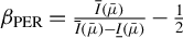
$\beta _{\text {PER}}=\frac {\overline {I}(\bar {\mu })}{\overline {I}(\bar {\mu })-\underline {I}(\bar {\mu })}-\frac {1}{2}$
 . Step 4 in the proof of Theorem 1(ii) shows that the only
$\Gamma $
 -MMR optimal rule of form
$d_{\text {step},\beta }$
 is
$d_{\text {step}}^*\neq d_{\text {PER}}^*$
 .
(ii) “If”: When randomization is not allowed,
Theorem 2(ii)
shows that
$d_{w,0}^*$
 is always
$\Gamma $
 -PER optimal. Under condition (3.17), Theorem 1(i) establishes that
$d_{w,0}^*$
 is
$\Gamma $
 -MMR optimal as well.
“Only if”: Again,
$d_{w,0}^*$
 is always
$\Gamma $
 -PER optimal when randomization is not allowed. If (3.17) fails (i.e., (3.3) holds) and
$n>1$
 , it follows by Theorem 1(iv) that the randomized rule
$d_{w_{t^*},0}^*$
 is
$\Gamma $
 -MMR optimal. If
$n=1$
 , Theorem 1(iii) implies that
$d_{w,0}^*$
 is not optimal even among linear threshold rules.
Therefore, when (3.3)
holds,
$\Gamma $
 -MMR and
$\Gamma $
 -PER optimal rules disagree with and without
randomization.
B TECHNICAL LEMMAS SUPPORTING EX-ANTE ANALYSIS
Lemma B.1. The Bayes rule supported by prior (A.1) is
$d_{w,0}^*$
 .
Proof. Note
$\overline {I}(\bar {\mu })>0$
 due to
$\overline {I}(\bar {\mu })+\underline {I}(\bar {\mu })>0$
 and
$\underline {I}(-\bar {\mu })=-\overline {I}(\bar {\mu })$
 by Lemma D.1. Given
$\pi ^{*}$
 , the Bayes optimal rule must solve the posterior
problem

where
$f(Y|\bar {\mu })$
 and
$f(Y|-\bar {\mu })$
 are the likelihood of Y at
$\bar {\mu }$
 and
$-\bar {\mu }$
 . This problem is equivalent to

Since
$\overline {I}(\bar {\mu })>0$
 , the unique Bayes optimal rule is
$\mathbf {1}\{f(Y|-\bar {\mu })-f(Y|\bar {\mu })\leq 0\}$
 , which is equivalent to
$d^*_{w,0}$
 after further algebra.
Lemma B.2. Consider decision rule
$d^*_{w,0}$
 and prior
$\pi ^{*}$
 defined in (A.1). If (3.2) holds, then

Proof. As
$w^{\top }Y\sim N(w^{\top }\mu ,w^{\top }\Sigma w)$
 , algebra shows

for all
$\mu \in M$
 . In particular,

It follows that

and

So, (B.1) holds as long as
-
(i) $\overline {I}(\bar {\mu })\Phi \left (-\frac {w^{\top }\bar {\mu }}{\sqrt {w^{\top }\Sigma w}}\right )\geq -\underline {I}(\bar {\mu })\Phi \left (\frac {w^{\top }\bar {\mu }}{\sqrt {w^{\top }\Sigma w}}\right ),$
-
(ii) $\overline {I}(-\bar {\mu })\Phi \left (\frac {w^{\top }\bar {\mu }}{\sqrt {w^{\top }\Sigma w}}\right )\leq -\underline {I}(-\bar {\mu })\Phi \left (-\frac {w^{\top }\bar {\mu }}{\sqrt {w^{\top }\Sigma w}}\right ),$


both of which are the same as (3.2) after further algebra, recalling
that
$\overline {I}(-\bar {\mu })=-\underline {I}(\bar {\mu })$
 and
$-\underline {I}(-\bar {\mu })=\overline {I}(\bar {\mu })$
 by Lemma D.1,
$w=\Sigma ^{-1}\bar {\mu }$
 , and
$\lVert w \lVert _{\Sigma } =\sqrt {\bar {\mu }^{\top }\Sigma ^{-1}\bar {\mu }}$
 .
Lemma B.3. Consider the prior
$\pi ^{*}$
 such that
$\mu \sim \mathrm {unif}(\{-\bar {\mu },\bar {\mu }\})$
 , and when
$\mu =\bar {\mu }$
 ,

where
$p_{1}$
 is such that
$p_{1}\overline {I}(\bar {\mu })+(1-p_{1})\underline {I}(\bar {\mu })=0$
 , and when
$\mu =-\bar {\mu }$
 ,

where
$p_{2}$
 is such that
$p_{2}\overline {I}(-\bar {\mu })+(1-p_{2})\underline {I}(-\bar {\mu })=0$
 . Given this prior, any decision rule is Bayes optimal
under (3.3).
Proof. As (3.3) holds, we have
$\underline {I}(\bar {\mu })<0<\overline {I}(\bar {\mu })$
 . Analogous to Lemma B.1, a Bayes rule must solve

Since
$p_{1}\overline {I}(\bar {\mu })+(1-p_{1})\underline {I}(\bar {\mu })=0$
 and
$p_{2}\overline {I}(-\bar {\mu })+(1-p_{2})\underline {I}(-\bar {\mu })=0$
 , the objective is constant in a,
hence the claim.
Lemma B.4. Consider the prior
$\pi ^{*}$
 such that
$\mu \sim \mathrm {unif}(\{-\bar {\mu },\bar {\mu }\})$
 , when
$\mu =\bar {\mu }$
 ,

where
$p_{1}$
 is such that
$p_{1}\overline {I}(\bar {\mu })+(1-p_{1})\underline {I}(\bar {\mu })=0$
 , and when
$\mu =-\bar {\mu }$
 ,

where
$p_{2}$
 is such that
$p_{2}\overline {I}(-\bar {\mu })+(1-p_{2})\underline {I}(-\bar {\mu })=0$
 . Then, when (3.3) holds, we have

for any decision rule
$d\in \mathcal {D}_{n}$
 such that (A.2) is true.
Proof. Note again that (3.3)
implies
$\underline {I}(\bar {\mu })<0$
 and
$\overline {I}(\bar {\mu })>0$
 . For any decision rule
$d\in \mathcal {D}_{n}$
 such that (A.2) is true, algebra shows


implying
$\sup _{\pi \in \Gamma }r(d,\pi )=-\frac {\overline {I}(\bar {\mu })\underline {I}(\bar {\mu })}{\overline {I}(\bar {\mu })-\underline {I}(\bar {\mu })}$
 . Meanwhile, for any
$d\in \mathcal {D}_{n}$
 such that (A.2) is true, we may also calculate the following that
yields the desired conclusion:

Lemma B.5. In case (3.3), the function

is decreasing in
$[0,c^{*}]$
 and increasing in
$[c^{*},\infty )$
 .
Proof. Note when
$c\in [0,c^{*})$
 and (3.3) holds, we have
$-\underline {I}(\bar {\mu })>0$
 ,

and therefore,

and

When
$c=c^{*}$
 , note
$\overline {I}(\bar {\mu })\Phi \left (\frac {-\lVert w \lVert _{\Sigma } ^{2}+c^{*}}{\lVert w \lVert _{\Sigma } }\right )=-\underline {I}(\bar {\mu })\Phi \left (\frac {\lVert w \lVert _{\Sigma } ^{2}-c^{*}}{\lVert w \lVert _{\Sigma } }\right )$
 and

When
$c\in (c^{*},\infty )$
 , note

so that

and

Having shown that
$\frac {\partial g(c)}{\partial c}<0$
 when
$c\in [0,c^{*})$
 and
$\frac {\partial g(c)}{\partial c}>0$
 when
$c\in (c^{*},\infty )$
 , and since
$g(c)$
 is continuous at
$c=c^{*}$
 , we conclude that g is decreasing in
$[0,c^{*}]$
 and increasing in
$[c^{*},\infty )$
 .
Lemma B.6. In case (3.3) and when
$n>1$
 , let

and
$\dot {\mu }^{\top }\Sigma ^{-1}\bar {\mu }=0$
 . Then,
$\mathbb {E}_{\bar {\mu }}[d_{w_{t^{*}},0}(Y)]=\frac {\overline {I}(\bar {\mu })}{\overline {I}(\bar {\mu })-\underline {I}(\bar {\mu })}$
 , where
$t^{*}$
 is defined in (3.9).
Proof. Write
$f(t):=\mathbb {E}_{\bar {\mu }}[d_{w_{t},c}(Y)]=\Phi \left (\frac {w_{t}^{\top }\bar {\mu }}{\sqrt {w_{t}^{\top }\Sigma w_{t}}}\right )$
 and
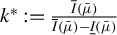
$k^{*}:=\frac {\overline {I}(\bar {\mu })}{\overline {I}(\bar {\mu })-\underline {I}(\bar {\mu })}$
 . Then, it suffices to show that
$f(t^{*})=k^{*}$
 , which is equivalent to showing

Furthermore, note

and

Therefore, substituting in these expressions,
$t^{*}$
 should be such that

As
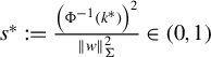
$s^{*}:=\frac {\left (\Phi ^{-1}(k^{*})\right )^{2}}{\lVert w \lVert _{\Sigma } ^{2}}\in (0,1)$
 due to (3.3), we can solve the above equation for
$t^{*}$
 , and after lengthy algebra, find that

C TECHNICAL LEMMAS SUPPORTING EX-POST ANALYSIS
Lemma C.1. Suppose all the conditions of Theorem 1 hold. If
$\underline {I}(\bar {\mu })<0<\overline {I}(\bar {\mu })$
 , then the unique
$\Gamma $
 -PER optimal rule is

Otherwise,
$d_{w,0}^{*}$
 is
$\Gamma $
 -PER optimal.
Proof. Let
$f(Y\mid \mu )$
 be the likelihood of Y. Then, for
each action
$a\in [0,1]$
 , we have

Therefore, when randomization is allowed, the
$\Gamma $
 -PER optimal rule can be found by solving

where

since
$\overline {I}(-\bar {\mu })=-\underline {I}(\bar {\mu })$
 and
$-\underline {I}(-\bar {\mu })=\overline {I}(\bar {\mu })$
 by Lemma D.1. Note that, for each action
$a\in [0,1]$
 ,

where
$\overline {I}(\bar {\mu })-\underline {I}(\bar {\mu })\geq 0$
 and
$\overline {I}(\bar {\mu })>0$
 due to our normalization
$\overline {I}(\bar {\mu })+\underline {I}(\bar {\mu })>0$
 . The conclusion follows from discussing the following
two cases.
Case 1:
$\boldsymbol {\underline {I}(\bar {\mu })\geq 0.}$

In this case,
$\frac {-\underline {I}(\bar {\mu })}{\overline {I}(\bar {\mu })-\underline {I}(\bar {\mu })} \leq a\leq \frac {\overline {I}(\bar {\mu })}{\overline {I}(\bar {\mu })-\underline {I}(\bar {\mu })}$
 for all
$a\in [0,1]$
 . Thus, (C.1) becomes

The
$\Gamma $
 -PER optimal rule is
$\mathbb {\mathbf {1}}\left \{ f(Y\mid -\bar {\mu })-f(Y\mid \bar {\mu })\leq 0\right \} $
 , which is
$d_{w,0}^{*}$
 after further algebra.
Case 2:
$\boldsymbol {\underline {I}(\bar {\mu })<0<\overline {I}(\bar {\mu }).}$

In this case, we have (again, note
$\overline {I}(\bar {\mu })+\underline {I}(\bar {\mu })>0$
 ):

Therefore:
-
• When $a\in \left [0,\frac {-\underline {I}(\bar {\mu })}{\overline {I}(\bar {\mu })-\underline {I}(\bar {\mu })}\right )$
, $$ \begin{align*} V_{\Gamma}(a)= &\ f(Y\mid\bar{\mu})\overline{I}(\bar{\mu})(1-a)-f(Y\mid-\bar{\mu})\underline{I}(\bar{\mu})(1-a)\\ = &\ \underset{>0}{\underbrace{\left\{ f(Y\mid\bar{\mu})\overline{I}(\bar{\mu})+f(Y\mid-\bar{\mu})\left(-\underline{I}(\bar{\mu})\right)\right\} }}(1-a). \end{align*} $$
Thus, $V_{\Gamma }(\cdotp )$
is strictly decreasing in
$a\in \left [0,\frac {-\underline {I}(\bar {\mu })}{\overline {I}(\bar {\mu })-\underline {I}(\bar {\mu })}\right )$
. -
• When $a\in \left [\frac {-\underline {I}(\bar {\mu })}{\overline {I}(\bar {\mu })-\underline {I}(\bar {\mu })},\frac {\overline {I}(\bar {\mu })}{\overline {I}(\bar {\mu })-\underline {I}(\bar {\mu })}\right ),$
$$ \begin{align*} V_{\Gamma}(a)& = f(Y\mid\bar{\mu})\overline{I}(\bar{\mu})(1-a)+f(Y\mid-\bar{\mu})\overline{I}(\bar{\mu})a\\ & = f(Y\mid\bar{\mu})\overline{I}(\bar{\mu})+\underset{>0}{\underbrace{\overline{I}(\bar{\mu})}}\left(f(Y\mid-\bar{\mu})-f(Y\mid\bar{\mu})\right)a. \end{align*} $$
Thus, if $f(Y\mid -\bar {\mu })>f(Y\mid \bar {\mu })$
,
$V_{\Gamma }(\cdotp )$
is strictly increasing in
a, and if
$f(Y\mid -\bar {\mu })<f(Y\mid \bar {\mu })$
,
$V_{\Gamma }(\cdotp )$
is strictly decreasing in
a. When
$f(Y\mid -\bar {\mu })=f(Y\mid \bar {\mu })$
,
$V_{\Gamma }(\cdotp )$
is constant in a. -
• When $a\in \left [\frac {\overline {I}(\bar {\mu })}{\overline {I}(\bar {\mu })-\underline {I}(\bar {\mu })},1\right ]$
, $$ \begin{align*} V_{\Gamma}(a) & =\underset{>0}{\underbrace{(f(Y\mid-\bar{\mu})\overline{I}(\bar{\mu})-f(Y\mid\bar{\mu})\underline{I}(\bar{\mu}))}}~a, \end{align*} $$implying that $V_{\Gamma }(\cdotp )$
is strictly increasing in
a.
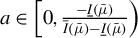


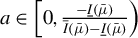








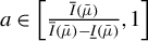


In sum, if
$f(Y\mid -\bar {\mu })>f(Y\mid \bar {\mu })$
 ,
$V_{\Gamma }(\cdotp )$
 is first strictly decreasing and then increasing, with
the minimum achieved at
$a=\frac {-\underline {I}(\bar {\mu })}{\overline {I}(\bar {\mu })-\underline {I}(\bar {\mu })}$
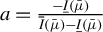 ; if
$f(Y\mid -\bar {\mu })<f(Y\mid \bar {\mu })$
 ,
$V_{\Gamma }(\cdotp )$
 is first strictly decreasing and increasing with the
minimum achieved at
$a=\frac {\overline {I}(\bar {\mu })}{\overline {I}(\bar {\mu })-\underline {I}(\bar {\mu })}$
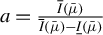 ; if
$f(Y\mid -\bar {\mu })=f(Y\mid \bar {\mu })$
 (which only happens in a null set),
$V_{\Gamma }(\cdotp )$
 achieves minimum at any point between
$[\frac {-\underline {I}(\bar {\mu })}{\overline {I}(\bar {\mu })-\underline {I}(\bar {\mu })},\frac {\overline {I}(\bar {\mu })}{\overline {I}(\bar {\mu })-\underline {I}(\bar {\mu })}]$
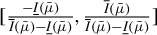 . Therefore, the unique
$\Gamma $
 -PER optimal rule is

Lemma C.2. Suppose all conditions of Theorem 1 hold true. Then,
$d_{w,0}^{*}$
 is always the
$\Gamma $
 -PER optimal non-randomized rule.
Proof. When randomization is not allowed, we need to solve (by a similar
derivation to Lemma C.1)
$\inf _{a\in \{0,1\}}V_{\Gamma }(a)$
 , where
$V_{\Gamma }(a)$
 is defined in (C.1). As

the optimal action would be
$a=1$
 if and only if
$V_{\Gamma }(1)\leq V_{\Gamma }(0)$
 , which is equivalent to
$d_{w,0}^{*}$
 after further algebra.
D ADDITIONAL RESULTS
Lemma D.1. Consider a treatment choice problem with welfare function (2.1), statistical model (2.3), and a set of priors (2.9), which satisfy Assumption 1. Then, the following statements hold:
-
(i) $\overline {I}(-\bar {\mu })=-\underline {I}(\bar {\mu })$
,
$\underline {I}(-\bar {\mu })=-\overline {I}(\bar {\mu })$
; -
(ii) $\overline {I}(-\bar {\mu })+\underline {I}(-\bar {\mu })=-(\underline {I}(\bar {\mu })+\overline {I}(\bar {\mu }))$
.



Proof.
Statement (i). Here, we only show that
$\overline {I}(-\bar {\mu })=-\underline {I}(\bar {\mu })$
 . An analogous argument proves
$\underline {I}(-\bar {\mu })=-\overline {I}(\bar {\mu })$
 . By definition,

Since
$\Theta $
 is centrosymmetric and both
$U(\cdotp )$
 and
$m(\cdot )$
 are linear, we have

as required.
Statement (ii). Directly follows from summing both equalities in statement (i).
Lemma D.2. In Example 1,
suppose
$k>\sqrt {\frac {\pi }{2}}\sigma $
 . Then, if
$\bar {\mu }>0$
 is sufficiently small, the corresponding
$\Gamma $
 -PER optimal rule is dominated in terms of profiled
regret.
Proof. Denote by
$d_{MMR,\text {linear}}^{*}$
 the least randomizing global MMR optimal rule derived
in Montiel Olea et al. (Reference Montiel Olea, Qiu and Stoye2026). We
aim to show that when
$k>\sqrt {\frac {\pi }{2}}\sigma $
 and
$\bar {\mu }>0$
 is sufficiently small, the associated
$\Gamma $
 -PER optimal rule
$d^*_{\text {PER}}$
 is such that

with the inequality strict for all
$\mu>0$
 . A symmetry argument then immediately implies that
$d_{\mathrm {PER}}^{*}$
 is dominated in terms of profiled regret.
Step 1: Pick any
$0<\bar {\mu }<\sqrt {\frac {\pi }{2}}\sigma $
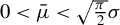 . We show that
$\bar {R}(d_{\mathrm {PER}}^{*},\mu )=(\mu +k)\left (1-\mathbb {E}_{\mu }\left [d_{\mathrm {PER}}^{*}(\hat {\mu })\right ]\right )$
 for all
$\mu \geq 0$
 . By results in Montiel Olea et al. (Reference Montiel Olea, Qiu and Stoye2026, Appendix B.3.1), we may write the
profiled regret of a rule d as

Thus, it suffices to show

for any
$0\leq \mu \leq k$
 . As
$\sqrt {\frac {\pi }{2}}\sigma <k$
 , Corollary 2 implies that the corresponding
$\Gamma $
 -PER rule for any
$0<\bar {\mu }<\sqrt {\frac {\pi }{2}}\sigma $
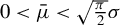 is

and further algebra shows
$\mathbb {E}_{\mu }\left [d_{\mathrm {PER}}^{*}(\hat {\mu })\right ]=\frac {1}{2}+\frac {\overline {\mu }}{2k}\left (1-2\Phi \left (-\frac {\mu }{\sigma }\right )\right )$
 . Then,

if and only if

which is equivalent to

Note the left-hand side of (D.2) is increasing in
$\mu $
 , and
$\lim _{\mu \downarrow 0}\left (\frac {\mu }{\left (1-2\Phi \left (-\frac {\mu }{\sigma }\right )\right )}\right )=\frac {\sigma }{2\phi \left (0\right )}=\sigma \sqrt {\frac {\pi }{2}}>\overline {\mu }$
 . As
$0<\bar {\mu }<\sqrt {\frac {\pi }{2}}\sigma $
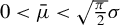 , we conclude that (D.2) indeed holds, and it follows

for all
$\mu \geq 0$
 . As a result, we conclude that, for any
$0<\bar {\mu }<\sqrt {\frac {\pi }{2}}\sigma $
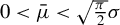 , we have

Step 2: We show that
$\bar {R}(d_{\mathrm {PER}}^{*},\mu )$
 is strictly increasing in
$\mu $
 for any
$0<\bar {\mu }<\sqrt {\frac {\pi }{2}}\sigma $
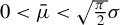 small enough. To see this, note

in which note (1):
$0<1-2\Phi \left (-\frac {\mu }{\sigma }\right )\leq 1$
 for all
$\mu \geq 0$
 and
$(2)$
 :
$2(\mu +k)\frac {1}{\sigma }\phi \left (\frac {\mu }{\sigma }\right )>0$
 is first increasing and then decreasing with a unique
and finite maximum
$C_{k}>0$
 . Therefore, we conclude that for any
$0<\overline {\mu }<\min \left (\frac {k}{\left (1+C_{k}\right )},\sqrt {\frac {\pi }{2}}\sigma \right )$
 , we have
$\frac {\partial \bar {R}(d_{\mathrm {PER}}^{*},\mu )}{\partial \mu }>0$
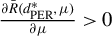 for all
$\mu \geq 0$
 . That is,
$\bar {R}(d_{\mathrm {PER}}^{*},\mu )$
 is strictly increasing in
$\mu \in [0,\infty ]$
 .
Step 3: Montiel Olea et al. (Reference Montiel Olea, Qiu and Stoye2026) have already shown that

Then, by the conclusion from step 3 and noting
$\bar {R}(d_{\mathrm {PER}}^{*},0)=\frac {k}{2}$
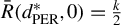 , we see that (D.1) indeed holds with the inequality
strict for all
$\mu>0$
 , completing the proof.
E GENERAL NATURE OF OUR MAIN RESULTS
In the main text, we derived finite-sample
$\Gamma $
 -MMR and -PER optimal rules for a class of priors such that
$\pi _{\mu }\sim \text {unif } {\left (\left \{ -\overline {\mu },\overline {\mu }\right \} \right )}$
 . In this section, we discuss the implications of our results
when
$\pi _{\mu }$
 has a more general structure (e.g., with a continuous
support).
It is relatively straightforward to extend our
$\Gamma $
 -PER results (Theorem 2) to other forms of
$\pi _{\mu }$
 . Let

The ex-post
$\Gamma $
 -PER criterion aims to solve
$\min _{a\in [0,1]}V_{\Gamma }(a).$
 Given a general
$\pi _{\mu }$
 and the normal likelihood of Y, we can derive
the posterior distribution of the reduced-form parameter
$\mu $
 given Y, written as
$\pi _{\mu \mid Y}$
 , using the standard Bayes rule. In light of the structure of
the class of priors
$\Gamma $
 , we see

Note
$\overline {I}(x)\left (1-a\right )\geq -\underline {I}(x)a$
 if and only if
$\overline {I}(x)\geq a\left (\overline {I}(x)-\underline {I}(x)\right )$
 , equivalent to (assuming
$\overline {I}(x)-\underline {I}(x)>0$
 for all x in the support of
$\pi _{\mu \mid Y}$
 )
$a\leq \frac {\overline {I}(x)}{\overline {I}(x)-\underline {I}(x)}.$
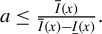 Thus, for each
$a\in [0,1]$
 , we have

The key observation is that the value of
$V_{\Gamma }(a)$
 for each
$a\in [0,1]$
 can be numerically solved, although it may not have a
closed-form solution. Therefore, in general, we can still find
$d_{\text {PER}}^{*}(Y)$
 by numerically solving
$\min _{a\in [0,1]}V_{\Gamma }(a)$
 . Note as the solution of
$\min _{a\in [0,1]}V_{\Gamma }(a)$
 may or may not be at the corners
$\{0,1\}$
 , it is in general not the case that the
associated
$\Gamma $
 -PER rule always randomizes.
In contrast, the
$\Gamma $
 -MMR optimal rule is more difficult to find once we allow
general forms of
$\pi _{\mu }$
 . Similar to the unconstrained MMR optimality problem, one
often needs to resort to the “guess-and-verify” strategy by
forming a least favorable prior—unlike the unconstrained scenario, for
the
$\Gamma $
 -MMR problem, the LFP has to come from
$\Gamma $
 , which restricts Nature’s strategy significantly. The
particular form of
$\pi _{\mu }\sim \text {unif } {\left (\left \{ -\overline {\mu },\overline {\mu }\right \} \right )}$
 makes our guess of the LFP much easier, while for other cases,
it may be more difficult. That said, although the exact analytic form of
$\Gamma $
 -MMR optimal rule is difficult to acquire for general
$\pi _{\mu }$
 , one may utilize recent computational techniques (Aradillas
Fernández et al., Reference Aradillas Fernández, Blanchet, Olea, Qiu, Stoye and Tan2025;
Guggenberger and Huang, Reference Guggenberger and Huang2025) to
numerically find an approximately
$\Gamma $
 -MMR optimal rule. find an
$\varepsilon $
 -
$\Gamma $
 -MMR optimal rule with near optimal convergence property.
Moreover, we think that the main qualitative insights regarding
$\Gamma $
 -MMR optimal rules may extend to other forms of
$\pi _{\mu }$
 . For example, we conjecture that whenever the identification
power of the model is sufficiently large compared to the informativeness of the
data (in a sense to be suitably defined),
$\Gamma $
 -MMR optimal rule will take a form of a non-randomized
threshold rule; otherwise, the optimal rule may be randomized. We leave the
verification of these conjectures for future research.
FUNDING STATEMENT
This study was funded by the NSF (Grant No. SES-2315600).
COMPETING INTEREST STATEMENT
The authors declare that no competing interests exist.





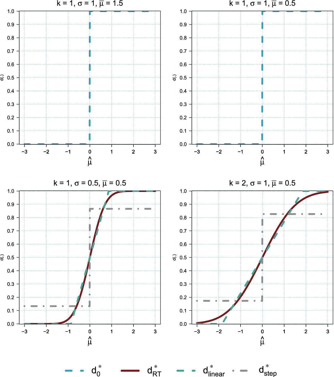


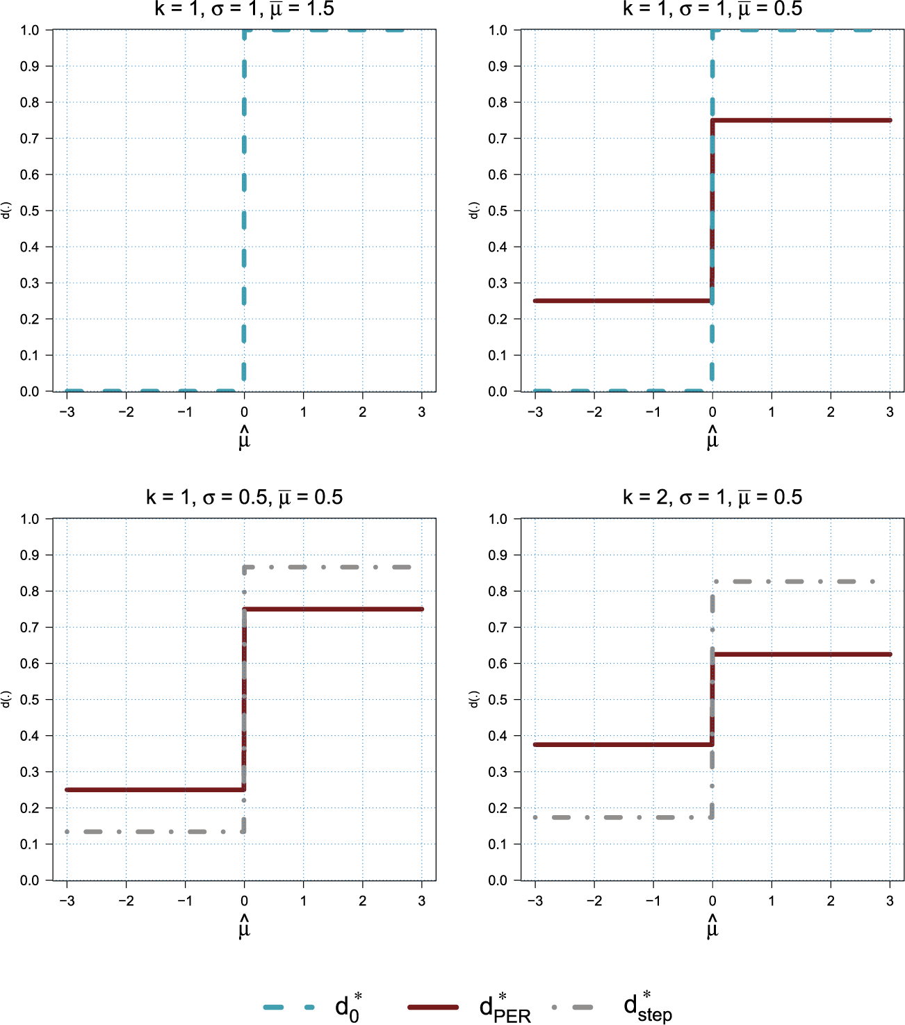


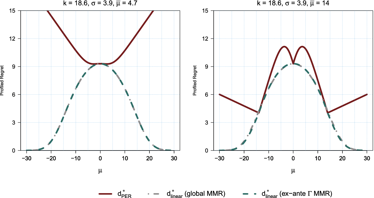


 Open access

