



1. Introduction
Coherent structures, as a valuable approach for revealing the flow physics underlying complex phenomena of turbulent flows, have attracted considerable interest over many years (Jeong et al. Reference Jeong, Hussain, Schoppa and Kim1997; del Álamo et al. Reference del Álamo, Jiménez, Zandonade and Moser2006; Adrian Reference Adrian2007; Ringuette et al. Reference Ringuette, Wu and Martín2008; Lozano-Durán & Jiménez Reference Lozano-Durán and Jiménez2014; Baars et al. Reference Baars, Hutchins and Marusic2017; Hwang & Sung Reference Hwang and Sung2018; Motoori & Goto Reference Motoori and Goto2021; Chen et al. Reference Chen, Cheng, Gan and Fu2023; Li et al. Reference Li, Fu and Xu2025). They offer a more intuitive and fundamental perspective on understanding the turbulence dynamics than the Navier–Stokes (NS) equations themselves. Jiménez (Reference Jiménez2018) comprehensively reviewed coherent structures in incompressible flows, detailing their conceptual definitions, physical existence, detection methodologies, experimental evidence and theoretical modelling. In the current study, the wall-bounded compressible turbulent flows are considered. Based on the variables analysed, coherent structures can be classified into different categories, such as intense fluctuation structures (i.e. streaks), Qs (quadrant events) structures and vortex clusters. Although these three types of structures are identified from velocity/temperature fluctuations, Reynolds stress/turbulent heat flux and vortex criterion (i.e. Q criterion) fields, they are highly correlated in both turbulent channel flows (Lozano-Durán et al. Reference Lozano-Durán, Flores and Jiménez2012; Li et al. Reference Li, Fu and Xu2025) and turbulent boundary layers (Dong et al. Reference Dong, Tong, Yu, Chen, Yuan and Wang2022b ), which can be directly observed using the conditional average method. They all play important roles in the self-sustaining process of turbulence near the wall.
In the regime of wall-bounded incompressible turbulent flows, the understanding of coherent structures is quite comprehensive, particularly with regards to their spatial characteristics. For the intense streamwise velocity fluctuation structures, the geometrical scale is widely concerned. Near-wall streamwise streaks are small-scale, elongated structures. Classified according to the instantaneous streamwise velocity, they can be divided into high-speed streaks and low-speed streaks. Both types exhibit a common spanwise spacing of nearly 100 wall units. As the Reynolds number rises, large-scale motions (LSMs) and even very large-scale motions (VLSMs) become observable. These structures are of crucial significance in momentum and energy transfer, and interact with the near-wall small-scale structures (Mathis et al. Reference Mathis, Hutchins and Marusic2009; Ganapathisubramani et al. Reference Ganapathisubramani, Hutchins, Monty, Chung and Marusic2012; Hwang et al. Reference Hwang, Lee, Sung and Zaki2016; Zhou et al. Reference Zhou, Xu and Jiménez2022). Hairpin packets are among the most intensively studied large-scale motions. Adrian (Reference Adrian2007) carried out a systematic investigation of hairpin vortices in turbulent boundary layers and discovered that packets consisting of 5–10 hairpin vortices have a streamwise length of approximately 2–3 times
 $\delta$
(where
 $\delta$
denotes the boundary layer thickness). Regarding VLSMs, in channel flows, their length can reach nearly
 $30h$
(
 $h$
represents the channel half-height) (Monty et al. Reference Monty, Stewart, Williams and Chong2007), while in turbulent boundary layers, it can reach
 $10$
to
 $15\delta$
(Hutchins & Marusic Reference Hutchins and Marusic2007). In addition, investigations on the size and shape of Qs structures have been conducted (Lozano-Durán et al. Reference Lozano-Durán, Flores and Jiménez2012), and self-similar properties in the logarithmic layer provide evidence for Townsend’s attached-eddy hypothesis (Townsend Reference Townsend1976).
As for the time-resolved evolution of coherent structures, related research is quite limited due to the high time resolution required, which imposes significant demands on data storage. The large volume of stored data also poses a major challenge for post-processing analysis, as data reading can become a bottleneck for processing speed. Lozano-Durán & Jiménez (Reference Lozano-Durán and Jiménez2014) carefully studied the full-life evolution of Qs structures using a tracking method in turbulent channel flows. As noted by the authors, several special designs have been proposed for data storage. The most impressive finding is that the attached Qs structures have lifetimes proportional to their distance from the wall, which fills a gap in the understanding of the time scales of coherent structures in channel flows. Furthermore, advection velocities have also been investigated and the results show that they are close to the mean velocity of the flow field above the buffer layer. This same approach was also employed by Cardesa et al. (Reference Cardesa, Vela-Martín and Jiménez2017) to investigate homogeneous isotropic turbulence. However, the above-mentioned analyses of the temporal evolution of coherent structures have not been applied to other types of wall-bounded flows, such as turbulent boundary layers, which are more challenging.
For compressible flows, research on coherent structures (Ganapathisubramani et al. Reference Ganapathisubramani, Clemens and Dolling2006; Ringuette et al. Reference Ringuette, Wu and Martín2008; Pirozzoli & Bernardini Reference Pirozzoli and Bernardini2011; Bross et al. Reference Bross, Scharnowski and Kähler2021; Chen et al. Reference Chen, Cheng, Gan and Fu2023; Zhou et al. Reference Zhou, Wang, Zhang, Huang and Xu2024; Li et al. Reference Li, Fu and Xu2025) is far more preliminary than that in incompressible flows. Ganapathisubramani et al. (Reference Ganapathisubramani, Clemens and Dolling2006) employed the wide-field particle image velocimetry method to observe coherent structures at Mach number 2 and reported that the streamwise length of the velocity streaks exceeds 8
 $\delta$
. Bross et al. (Reference Bross, Scharnowski and Kähler2021) conducted experiments on flat-plate flow under various Reynolds and Mach numbers to analyse the effects of compressibility. The results of correlation and spectral analyses indicate that compressibility slightly elongates the wavelengths of the most energetic frequencies and increases the spanwise spacing of large-scale structures. In addition to experiments, direct numerical simulation (DNS) is also a crucial approach. Using DNS, it has been found that near-wall streaks in compressible flows are elongated due to density and temperature gradients (Coleman et al. Reference Coleman, Kim and Moser1995) or cold isothermal wall conditions (Duan et al. Reference Duan, Beekman and MartÍN2010). Ringuette et al. (Reference Ringuette, Wu and Martín2008) observed that some low-speed structures in turbulent boundary layers can have streamwise lengths up to
 $100\delta$
at a Mach number of 3. Zhou et al. (Reference Zhou, Wang, Zhang, Huang and Xu2024) investigated the influence of LSMs on near-wall structures in compressible turbulent channel flows and proposed that the spanwise drifting of near-wall solenoidal streaks is driven by LSMs, whereas the drifting of near-wall dilatational structures, which is faster, does not primarily result from the influence of LSMs.
Until now, the focus has been primarily on coherent structures associated with velocity. However, the temperature field, which has attracted significant interest (Walz Reference Walz1969; Huang et al. Reference Huang, Coleman and Bradshaw1995; Zhang et al. Reference Zhang, Bi, Hussain and She2013; Cheng et al. Reference Cheng, Chen, Zhu, Wei and Fu2024), represents a distinctive feature of compressible flows since it is coupled with velocity fields. The existing literature on coherent structures associated with temperature remains highly limited. Yuan et al. (Reference Yuan, Tong, Li, Chen and Dong2022) examined fluctuating temperature structures in supersonic turbulent boundary layers over cooled and heated walls. Bai et al. (Reference Bai, Cheng and Fu2024) identified temperature structures based on the well-established Townsend’s attached-eddy hypothesis and analysed their inclination angles, revealing a statistical similarity between velocity and temperature structures. Moreover, the inner–outer interaction characteristic observed in velocity structures is also present between small- and large-scale temperature structures (Pirozzoli & Bernardini Reference Pirozzoli and Bernardini2011). Additionally, Dong et al. (Reference Dong, Tong, Yu, Chen, Yuan and Wang2022a , Reference Dong, Tong, Yu, Chen, Yuan and Wang b ) investigated turbulent heat flux structures in compressible turbulent boundary layers and found that these structures exhibit distinct asymmetrical features compared with Reynolds shear stress structures. Li et al. (Reference Li, Fu and Xu2025) systematically investigated the spatial and shape characteristics of intense velocity and temperature structures, as well as the Qs structures of Reynolds shear stress and turbulent heat flux in turbulent channel flows, considering the effects of Reynolds and Mach numbers, and provided an explanation for the differences between velocity and temperature structures.
The paper is organised as follows. Section 2 presents the direct numerical simulation cases conducted and used for analysis, along with the numerical methods employed to solve the governing equations. It also introduces the methodology for structure identification and defines key geometrical parameters of the structures. Furthermore, given the interest in temporal evolution, the approach for determining the lifetime evolution of structures is described in detail. The spatial characteristics of intense velocity and temperature fluctuation structures are discussed in § 3, while § 4 examines their temporal characteristics, including advection velocity, lifetime and birth/death. Section 5 presents the evolution of the position and shape of the attached structures over their entire lifetime. Conclusions are presented in § 6.
2. Methodology and numerical set-up
2.1. Simulation settings
The compressible NS equations for ideal gas are employed in the present study:
 \begin{equation} \frac {{\partial \rho }}{{\partial t}} + \frac {{\partial \rho {u_{\!j}}}}{{\partial {x_{\!j}}}} = 0, \end{equation}
 \begin{equation} \frac {{\partial \rho {u_i}}}{{\partial t}} + \frac {{\partial \rho {u_i}{u_{\!j}}}}{{\partial {x_{\!j}}}} = - \frac {{\partial p}}{{\partial {x_i}}} + \frac {{\partial {\tau _{ij}}}}{{\partial {x_{\!j}}}}, \end{equation}
 \begin{equation} \frac {{\partial \rho E}}{{\partial t}} + \frac {{\partial \rho H{u_{\!j}}}}{{\partial {x_{\!j}}}} = \frac {{\partial {\tau _{ij}}{u_i}}}{{\partial {x_{\!j}}}} - \frac {{\partial {q_{\!j}}}}{{\partial {x_{\!j}}}}, \end{equation}
where
 $x_i(i = 1, 2, 3) = (x, y, z), u_i(i = 1, 2, 3) = (u, v, w)$
and
 \begin{equation} {\tau _{ij}} = \mu \left ( {\frac {{\partial {u_i}}}{{\partial {x_{\!j}}}} + \frac {{\partial {u_{\!j}}}}{{\partial {x_i}}} - \frac {2}{3}\frac {{\partial {u_k}}}{{\partial {x_k}}}{\delta _{ij}}} \right )\!,\quad {q_{\!j}} = - \kappa \frac {{\partial T}}{{\partial {x_{\!j}}}}. \end{equation}
Here,
 $t$
denotes time, and
 $u$
,
 $v$
and
 $w$
are the velocity components in the streamwise (
 $x$
), wall-normal (
 $y$
) and spanwise (
 $z$
) directions, respectively. The
 $\rho ,T,p$
represent fluid density, temperature and pressure that satisfy the ideal gas law
 $p=\rho RT$
, where
 $R$
is the gas constant. Furthermore,
 $E = {u_i}{u_i} /2+ {C_v}T$
is the total energy and the total enthalpy is defined as
 $H = E + p/\rho$
;
 $\tau _{ij}$
denotes the viscous stress tensor, where
 $\mu$
is the dynamic viscosity obeying Sutherland’s law; and
 $q_{\!j}$
is the heat flux. Additionally, the heat conductivity coefficient
 $\kappa = (C_{\!p}\mu) / Pr$
, and
 $C_v$
and
 $C_{\!p}$
stand for the constant-volume specific heat capacity and the constant-pressure specific heat capacity. The ratio of specific heat
 $\gamma = C_{\!p}/C_v = 1.4$
and the Prandtl number
 $Pr = 0.72$
. In the current study,
 $\bar \varphi$
denotes the Reynolds average of a generic variable
 $ \varphi$
and the corresponding fluctuation is
 $\varphi '$
. These equations are solved using the open-source GPU-based code STREAmS (Bernardini et al. Reference Bernardini, Modesti, Salvadore and Pirozzoli2021). A high-order kinetic-energy-preserving (KEP) scheme, which combines the sixth-order energy-preserving central scheme with the seventh-order weighted essentially non-oscillatory (WENO) scheme, is employed to discretise the convective terms, while the viscous terms are approximated using a sixth-order central scheme. Time integration is advanced via a three-stage, third-order Runge–Kutta (RK) scheme. The digital filter (DF) method of Klein et al. (Reference Klein, Sadiki and Janicka2003) is employed for inflow turbulence generation. Moreover, no–slip and isothermal boundary conditions are applied at the wall, while non-reflecting conditions are imposed at the far-field and outflow boundaries.
In the current study, two DNSs of compressible turbulent boundary layers (CTBLs) with friction Reynolds number
 $\textit{Re}_\tau$
up to 1000 have been conducted on adiabatic and cooled walls, respectively. The detailed parameters are summarised in table 1. Appendix A presents the wall-normal profiles of first- and second-order statistics in comparison with reference data for adiabatic wall conditions at
 ${\textit{Ma}}=2$
(Pirozzoli & Bernardini Reference Pirozzoli and Bernardini2011). The settings of the computational domain and mesh resolution involve a trade-off among the extremely high storage demands associated with capturing the time-resolved evolution of coherent structures, the fidelity of turbulence simulation, the emergence of large-scale structures and computational costs. As a result, the total storage used for these cases is approximately 50 TB, yielding over
 $5.5\times 10^5$
attached structures and
 $3.0\times 10^6$
detached structures to guarantee the robustness of the statistical analysis. A short subdomain from the high-Reynolds-number region and long subdomain from the entire valid region are stored with short and relatively long time separations, respectively, as shown in table 2. The short subdomain is used for investigating the spatial characteristics and temporal evolution of near-wall structures. Its time resolution
 $\Delta t^+$
is set to unity, which is sufficient to resolve the evolution between consecutive fields in the near-wall region and is close to the value used by Lozano-Durán & Jiménez (Reference Lozano-Durán and Jiménez2014) in incompressible channel flow. For large-scale structures, on the one hand, the lifetime is sufficiently long, implying that these structures can travel a considerable distance in the streamwise direction. On the other hand, the requirement for time resolution is relaxed, as the time scale associated with these large structures is significantly larger. Therefore, the long subdomain is used for capturing the complete evolution of large-scale structures. This is one of the main challenges in investigating the temporal evolution of large-scale structures in turbulent boundary layers, a difficulty that does not arise in channel flows.
Simulation settings of the DNS cases. Subscripts ’
 $w$
’ and ’
 $\delta$
’ denote the values of variables on the wall and at the edge of boundary layer, respectively.
 $T_r$
denotes the recovery temperature defined as
 $T_r=T_{\infty }(1+0.5r(\gamma -1)Ma^2)$
with recovery coefficient
 $r=0.89$
, where
 $T_{\infty }$
is temperature at upper boundary.
 $L_x$
,
 $L_{\!y}$
and
 $L_z$
are the domain size in streamwise, wall-normal and spanwise direction,
 $\delta _{\textit{in}}$
is the inflow boundary layer thickness,
 $N_x$
,
 $N_{\!y}$
and
 $N_z$
the grid dimensions. The mesh resolutions are calculated at the station with
 $\textit{Re}_\tau \approx 1000$
.

Table 1. Long description
The table presents a comparison of parameters for two DNS cases of compressible turbulent boundary layers with friction Reynolds number up to 1000. It includes data for adiabatic and cooled wall conditions. The table has 2 rows and 8 columns. Column headers are: Case, Ma, Tw/Tr, (Lx x Ly x Lz)/δin, Nx x Ny x Nz, Δx+, Δy+,w Δz+. Row 1: Case M2T10, Ma 2.25, Tw/Tr 1.0, (Lx x Ly x Lz)/δin 73 x 6 x 5, Nx x Ny x Nz 4900 x 220 x 420, Δx+ 8.78, Δy+,w 0.75, Δz+ 7.01. Row 2: Case M2T05, Ma 2.25, Tw/Tr 0.5, (Lx x Ly x Lz)/δin 60 x 6 x 5, Nx x Ny x Nz 3960 x 222 x 520, Δx+ 8.99, Δy+,w 0.80, Δz+ 5.71.
Parameters of the sets of stored subdomains. Sets T10S and T10L belong to Case M2T10, while Sets T05S and T05L belong to Case M2T05.
 $L_x$
is the length of the subdomain in the streamwise direction.
 $\textit{Re}_\theta$
is the Reynolds number based on the momentum deficit thickness
 $\theta$
and
 $\textit{Re}_\tau$
is the friction Reynolds number. The time resolution
 $\Delta t^+$
is non-dimensionalised by the viscous units at the station with
 $\textit{Re}_\tau \approx 1000$
.
 $t_L$
is the duration of the stored time series,
 $\delta _{\textit{in}}$
is the inflow boundary layer thickness and
 $u_{\infty }$
is streamwise velocity at upper boundary.
 $N_{\textit{field}}$
denotes the number of stored flow fields.

Table 2. Long description
A table comparing parameters of stored subdomains in turbulent boundary layers. The table has 4 rows and 8 columns. Column headers are Set, Lx, Reθ, Reτ, Δt+, tL, Nfield, and Storage. Row labels are T10S, T10L, T05S, and T05L. Row 1: T10S, 16.8δin, 5646–6401, 936–1037, 1, 181δin/u∞, 5301, 10.1 TB. Row 2: T10L, 58.1δin, 3720–6447, 627–1044, 3, 181δin/u∞, 1767, 14.5 TB. Row 3: T05S, 16.5δin, 2265–2642, 929–1044, 1, 236δin/u∞, 5250, 12.1 TB. Row 4: T05L, 44.9δin, 1636–2652, 694–1053, 3, 236δin/u∞, 1749, 14.5 TB.
2.2. Structure identification
In the current study, the intense velocity fluctuation
 $u'$
and temperature fluctuation
 $T'$
structures are focused on. For turbulent boundary layer flows, the effects of the turbulence/non-turbulence interface (TNTI) should be considered to obtain proper structures in the outer layer (Hwang & Sung Reference Hwang and Sung2018; Yuan et al. Reference Yuan, Tong, Li, Chen and Dong2022). The kinetic energy criterion proposed by Chauhan et al. (Reference Chauhan, Philip, de Silva, Hutchins and Marusic2014) is used here to identify the TNTI. The threshold of kinetic energy
 $\bar k$
is set to 0.09 which is consistent with Hwang & Sung (Reference Hwang and Sung2018). However, this interface obtained by the kinetic energy criterion is not that appropriate to distinguish the temperature fluctuations. Therefore, similarly, the scalar energy of temperature
 $100(T/T_\infty -1)^2$
is defined to identify the temperature interface using a threshold value of 0.04. Further details can be found in Appendix B.1. Conditioned on the height of the interface
 $\delta _t(x,z)$
, the average of the variable
 $\phi$
can be obtained and expressed as
 $ \langle \phi \rangle _t(y,\delta _t)$
. The corresponding fluctuations
 $\phi ^t = \phi -\langle \phi \rangle _t$
can also be defined.
Fluctuation magnitudes are chosen as the criteria to identify these two structures
 \begin{equation} {u^t(\boldsymbol{x})} \gt {\alpha _u}{u^t_{\textit{rms}}(y,\delta _{t,u})} \quad \text{or} \quad {u^t(\boldsymbol{x})} \lt -{\alpha _u}{u^t_{\textit{rms}}(y,\delta _{t,u})}, \end{equation}
 \begin{equation} {T^t(\boldsymbol{x})} \gt {\alpha _T}{T^t_{\textit{rms}}(y,\delta _{t,T})} \quad \text{or} \quad {T^t(\boldsymbol{x})} \lt -{\alpha _T}{T^t_{\textit{rms}}(y,\delta _{t,T})}, \end{equation}
where
 $\boldsymbol{x}=(x,y,z)$
. This method, taking the wall-normal distance into consideration, has been widely applied to wall-bounded flows (del Álamo et al. Reference del Álamo, Jiménez, Zandonade and Moser2006; Lozano-Durán et al. Reference Lozano-Durán, Flores and Jiménez2012; Lozano-Durán & Jiménez Reference Lozano-Durán and Jiménez2014; Hwang & Sung Reference Hwang and Sung2018; Li et al. Reference Li, Fu and Xu2025). The coefficients
 $\alpha _u$
and
 $\alpha _T$
for velocity and temperature, respectively, can be obtained by percolation analysis, which is shown in Appendix B.2. Finally,
 $\alpha _u=\alpha _T=1.5$
is adopted in this study, which is the same as Hwang & Sung (Reference Hwang and Sung2018). Notably, the values of these coefficients make no qualitative differences for the identified structures, as also pointed out by both Lozano-Durán et al. (Reference Lozano-Durán, Flores and Jiménez2012) and Hwang & Sung (Reference Hwang and Sung2018). In addition, only structures with a volume larger than the cube of 30 wall units are considered for analysis to avoid the effects of numerical issues, as suggested by Del Álamo et al. (Reference del Álamo, Jiménez, Zandonade and Moser2006).
Diagram of the intense
 $u'$
structure from Set T10S.
 $l_x$
,
 $l_{\!y}$
and
 $l_z$
are the dimensions of the structure’s circumscribing box.
 $(x_c, y_c, z_c)$
denotes the gravity centre of the structure.
 $y_{\textit{max}}$
and
 $y_{\textit{min}}$
represent the maximum and minimum distances from the points of the structure to the wall. The colour of the structure represents the wall-normal distance of the corresponding point.

Figure 1 displays an intense
 $u'$
structure from Set T10S as an example, annotating the key geometric features considered in the current study. The circumscribing box of the structure has dimensions
 $l_x \times l_{\!y} \times l_z$
. The centre of gravity of the structure is located at
 $(x_c, y_c, z_c)$
, which is generally offset from the box centre. Furthermore,
 $y_{\textit{max}}$
and
 $y_{\textit{min}}$
represent the maximum and minimum distances from the structure’s points to the wall. With these definitions, the classification of coherent structures can be conducted. The definition of attached structures varies across previous research. Del Álamo et al. (Reference del Álamo, Jiménez, Zandonade and Moser2006) regarded structures with
 $y^+_{\textit{min}} \lt 20$
as attached, while Hwang & Sung (Reference Hwang and Sung2018) adopted the criterion that
 $y^+_{\textit{min}} \approx 0$
. As mentioned by Hwang & Sung (Reference Hwang and Sung2018), approximately 88 % of the attached
 $u'$
structures identified by
 $y^+_{\textit{min}} \lt 20$
have
 $y^+_{\textit{min}} \approx 0$
. Therefore, in the current study, the criterion that
 $y_{\textit{min}}$
equals the wall-normal distance of the first mesh point,
 $y_{th}$
, is adopted, as it is more practical: the fluctuation at the wall is zero and no point on the wall is regarded as part of any coherent structure. Accordingly, structures with
 $y_{\textit{min}} \gt y_{th}$
are referred to as detached structures. Furthermore, attached structures with
 $y^+_{\textit{max}} \gt 100$
are classified as tall attached structures. In addition, intense fluctuation structures characterised by positive fluctuations are referred to as positive structures and denoted by ‘+’, while negative structures, consisting of negative fluctuations, are denoted by ‘−’.
2.3. Tracking method
The key problem is to construct the connection between coherent structures in two consecutive flow fields, accounting for single, transfer, splitting and merging configurations. The single configuration consists of two types. (1) Some structures fail to identify a corresponding counterpart in the preceding or succeeding flow field, resulting in their isolation; this phenomenon is interpreted as birth or death events associated with the flow. (2) Structures located at the streamwise boundary of the computational domain or at the temporal boundaries of the flow time range are considered incomplete. Moreover, the transfer configuration involves only a single structure, although its size and shape may change over time. The other two configurations involve multiple structures and are considerably more complex.
The criterion is that if these two structures have spatial overlap after updating the position of the succeeding structure by subtracting the advection distance in the streamwise direction, they are considered connected. The investigation on streamwise advection velocity of coherent structures will be introduced in § 4.1. As mentioned by Lozano-Durán & Jiménez (Reference Lozano-Durán and Jiménez2014), although advection has already been taken into consideration, some connections between small-scale structures that are expected to exist can still not be constructed through this method. However, since its proportion is small, this tracking method represents a good balance between efficiency and performance. It should be noted that when first processing the results, the accurate advection velocity is unknown. Therefore, the averaged streamwise velocity
 $\bar u$
with the near-wall region corrected by a constant value can be used as the initial estimate of the advection velocity, and a single iteration is sufficient to achieve satisfactory results. Numerical tests show that the statistical results of structures tracking are not highly sensitive to the choice of advection velocity, and the advection velocity is determined from the maximum value of the probability density function (p.d.f.) at each wall-normal location.
After processing all the flow fields, a large graph is formed. Each node represents a coherent structure that contains a timestamp and the associated mesh points. The presence of an edge between two nodes in the graph indicates that the latter evolves from the former. In addition, each edge is assigned a weight to describe the intensity of the relationship between the nodes connected by it. This weight is defined as the ratio (
 $V_{o}/\Delta V$
) of the overlap volume (
 $V_{o}$
) between two connected nodes to the volume difference (
 $\Delta V$
) between them. The higher the weight, the more prominent is this edge. The weight defined here is the reciprocal of that defined by Lozano-Durán & Jiménez (Reference Lozano-Durán and Jiménez2014), but this difference has no effect on the following results and is introduced solely for convenience.
This large graph contains numerous subgraphs that form isolated cycles with no connections to other subgraphs. Each subgraph represents an evolutionary process of the structures it contains. For convenience, these subgraphs will be referred to as graphs later. To further investigate the lifetime of structures, graphs containing nodes with in-degree or out-degree greater than one are reconstructed by retaining only the incoming or outgoing edge that has the maximum weight associated with each node. After reconstruction, all the connections with types of splitting and merging do not exist anymore. Figure 2 displays this reconstruction process. Before reconstruction, Nodes 22, 23 and 25 form a merging configuration, while Nodes 18, 20 and 21, as well as Nodes 35, 37 and 38, form splitting configurations. The weights of the associated edges are also provided, as shown in figure 2(a). Figure 2(b) shows the results of the reconstruction, which contain four branches, each representing a distinct lifetime evolution of a structure. Considering the configurations of the first and last nodes, these branches can be classified into nine categories, as shown in table 3. It should be noted that branches containing nodes located at the streamwise boundaries of the domain or at the temporal boundaries of the flow time range are considered incomplete and excluded from the analysis in the current study. As table 3 shows, incomplete branches constitute a relatively small proportion of the total number of branches.
Types and counts of branches for all the sets of subdomains stored in the current study. B, D, M, S and I denote birth, death, merging, splitting and incomplete states, respectively. Incomplete states refer to nodes located at the streamwise boundaries of the domain or at the temporal boundaries of the flow time range.

Table 3. Long description
A table with 10 rows and 10 columns comparing counts of branches for different sets of subdomains. The columns are labeled B-D, B-M, S-D, S-M, B-I, S-I, I-D, I-M, and I-I. The rows are labeled T10L u’, T10L T’, T10S u’, T10S T’, T05L u’, T05L T’, T05S u’, T05S T’, T05S u’, and T05S T’. Each cell contains a numerical value representing the count of branches for the corresponding set and type. The table provides detailed counts for birth, death, merging, splitting, and incomplete states across different sets of subdomains.
Diagram of graph reconstruction from Case M2T10: (a) before reconstruction and (b) after reconstruction. The weights of selected critical edges involved in branch selection are displayed using red text, respectively. Flow time associated with the nodes increases from top to bottom.

The properties of an evolution branch are not as straightforward to define and compute as those of a single structure (node), since the properties of the structure vary to some extent throughout the entire evolution process, especially for large-scale structures that exhibit substantial variations in their volume and centre position. In the current study, the attached property of an evolution branch is defined as whether the bottom of the structure corresponding to this branch reaches the wall at least once during its lifetime, as the wall has already exerted a direct influence on its development – specifically by restricting its growth in the wall-normal (y-) direction. Furthermore, unless otherwise specified, the properties of attached branches are represented by the maximum value of the corresponding structure properties observed during the evolutionary process, whereas those of unattached branches are averaged across the entire lifetime. The method described here is developed within the Eulerian framework. Its extension to the Lagrangian framework will be pursued in future work.
3. Spatial characteristics
Since Townsend’s attached-eddy hypothesis provides the fundamental physical basis for the well-known logarithmic laws governing mean velocity and velocity variances (Perry & Chong Reference Perry and Chong1982), this section examines the distribution and shape characteristics of attached and detached intense
 $u'$
and
 $T'$
structures to assess their potential self-similarity and to elucidate the influence of wall cooling conditions using the Sets T10S and T05S, as these two sets feature higher temporal resolution and a sufficiently long streamwise domain for the following analysis in this section. Additionally, differences between the intense
 $u'$
and
 $T'$
structures are discussed, although the underlying mechanisms will be explored in future work. Table 4 displays the number and volume fractions of the different types of structures analysed in this section. The attached
 $u'$
structures account for approximately 65 % of the total structure volume, despite comprising less than 20 % of the number fraction, which is consistent with findings from previous studies (Hwang & Sung Reference Hwang and Sung2018; Li et al. Reference Li, Fu and Xu2025). In contrast to compressible channel flows, where the wall-normal gradients of streamwise velocity and temperature remain positive throughout the domain, in compressible boundary layer flows, the extent of regions with positive wall-normal temperature gradients increases as the wall cooling effect intensifies, since the near-wall temperature peak rises up. Consequently, as shown in table 4, intense
 $u'^-$
and
 $T'^+$
structures exhibit larger volume fractions, which is the main difference from the results of Li et al. (Reference Li, Fu and Xu2025). In this study, compressible channel flows are treated as ultimately cooled wall-bounded flows in which the temperature peak shifts outside the domain and are used for comparison with the boundary layer cases conducted here.
Number and volume fractions of the intense fluctuation structures in Sets T10S and T05S. Two numbers in the brackets represent the numbers or fractions of positive structures and negative structures, respectively.

Table 4. Long description
A table with 6 rows and 4 columns comparing the number and volume fractions of attached and detached intense structures in Sets T10S and T05S. The columns are labeled Set, Type, Total number (+,-), Number fraction (+,-), and Volume fraction (+,-). The rows are grouped by set and type, with values representing the number and fractions of positive and negative structures. Notable trends include the attached structures accounting for approximately 65 percent of the total structure volume despite comprising less than 20 percent of the number fraction.
3.1. Population density
The population density of the intense fluctuation structures is investigated to examine the existence of hierarchical length scales (Perry & Chong Reference Perry and Chong1982), which has been identified by Hwang & Sung (Reference Hwang and Sung2018) in incompressible boundary layers. The following formula provides the definition of population density:
 \begin{equation} n_s(l_{\!y}) = \frac {N_s(l_{\!y})}{mL_xL_z}, \end{equation}
in which
 $n_s$
is the population density,
 $N_s(l_{\!y})$
is the number of structures with the structure height of
 $l_{\!y}$
, m is the number of fields used to count the structure number, and
 $L_x, L_z$
are the streamwise and spanwise length of subdomains (see table 2).
Population density of the intense (a)
 $u'$
and (b)
 $T'$
structures with respect to their height in Set T10S. The slopes of the dashed lines are also displayed. The part of the lines near their right ends are smoothed to elucidate the trends, since the number of the large-scale structures is small which causes the original statistical data denoted by points to oscillate.

Population density of the intense (a)
 $u'$
and (b)
 $T'$
structures with respect to their height in Set T05S. The slopes of the dashed lines are also displayed. The part of the lines near their right ends are smoothed to elucidate the trends, since the number of the large-scale structures is small, which causes the original statistical data denoted by points to oscillate.

Figure 4. Long description
Two line graphs depict the population density of intense structures with respect to their height. Panel A: The line graph shows the population density of intense streamwise velocity fluctuation structures. The x-axis represents the height in wall units (l_y+) on a logarithmic scale ranging from 10^0 to 10^4. The y-axis represents the population density (n_s) on a logarithmic scale ranging from 10^-6 to 10^0. The graph includes three lines: Attached u’ (light blue), Attached u’’ (blue), and Detached u’ (gray). The slopes of the dashed lines are labeled as -2.3, -2.8, and -1.0. Panel B: The line graph shows the population density of intense temperature fluctuation structures. The x-axis represents the height in wall units (l_y+) on a logarithmic scale ranging from 10^0 to 10^4. The y-axis represents the population density (n_s) on a logarithmic scale ranging from 10^-6 to 10^0. The graph includes three lines: Attached T’’ (light red), Attached T’ (red), and Detached T’ (gray). The slopes of the dashed lines are labeled as -2.4, -1.0, and -1.1.
Figures 3 and 4 present the population densities of attached positive, attached negative and detached structures in Sets T10S and T05S. The dashed lines in these figures illustrate the decreasing trend in population density with increasing structure height, following an inverse power-law relationship
 $n_s \propto (l_{\!y}^+)^k$
, where
 $k$
denotes the slope of each dashed line, for
 $l_{\!y}^+ \gt 100$
beyond the buffer layer. The slope
 $k$
varies across different flows, although the theory of Perry & Chong (Reference Perry and Chong1982) indicates
 $k = -1$
. Cheng et al. (Reference Cheng, Li, Lozano-Durán and Liu2020) reported values of
 $-1.3$
for intense
 $u'^+$
structures and
 $-1.9$
for intense
 $u'^-$
in incompressible channel flows, whereas Hwang & Sung (Reference Hwang and Sung2018) observed the
 $-1$
scaling law for attached
 $u'$
structures without distinguishing their sign, within a limited range of
 $l_{\!y}^+$
in incompressible boundary layer flows, which is consistent with the current findings in figures 3(a) and 4(a) for attached
 $u'^+$
structures. Moreover, similar to Cheng et al. (Reference Cheng, Li, Lozano-Durán and Liu2020), attached
 $u'^-$
structures exhibit a higher decay rate than attached
 $u'^+$
structures in the logarithmic layer. In addition, the cooling effect of the wall appears to have no influence on the slope
 $k$
. Regarding intense temperature structures, previous research is scarce and Yuan et al. (Reference Yuan, Tong, Li, Chen and Dong2022) only reports variation trends primarily confined to the buffer layer, with
 $l_{\!y}^+ \lt 200$
. In the current study, the slope
 $k$
is nearly identical for attached
 $T'^+$
and
 $T'^-$
structures, and wall cooling reduces the value of
 $k$
. For Set T05S, attached
 $T'$
structures nearly follow the
 $-1$
scaling law shown in figure 4(b). Furthermore, detached structures also exhibit an inverse power-law behaviour, but with a significantly higher decay rate compared with attached structures.
The deviation from the
 $-1$
scaling law in the population density of attached structures may be attributed to three primary factors. First, the Reynolds number in the current study is insufficiently high, meaning that scale separation is not fully developed. Second, real flow structures interact with one another and cannot be treated as perfectly isolated entities, as assumed by Perry & Chong (Reference Perry and Chong1982). Third, Townsend’s attached-eddy hypothesis may not be perfectly valid in real flows for all types of structures. It highlights a critical area for refining existing theoretical assumptions and demonstrates the potential for future improvements in turbulence modelling.
3.2. Shape characteristics
The shape characteristics of the intense fluctuation structures are investigated in terms of the length-to-height and width-to-height aspect ratios, which are also regarded as indicators of self-similarity (del Álamo et al. Reference del Álamo, Jiménez, Zandonade and Moser2006; Lozano-Durán et al. Reference Lozano-Durán, Flores and Jiménez2012; Hwang & Sung Reference Hwang and Sung2018; Li et al. Reference Li, Fu and Xu2025). Importantly, the objective of this analysis is not to categorise the structures into idealised shapes, such as hairpin vortices, nor to reconstruct their exact geometric boundaries; such detailed topological characterisations fall outside the scope of the current study. Same as in § 3.1, attached positive, attached negative and detached structures are analysed separately, which also provides a perspective for unified consideration.
The structures from Set T10S with adiabatic wall condition are analysed first. It should be noted that the adiabatic wall condition is implemented by setting the wall temperature to the recovery temperature with a recovery coefficient
 $r=0.9$
. Therefore, this adiabatic condition is not strictly satisfied and results show that a tiny negative wall-normal gradient of temperature occurs close to the wall. This configuration can be regarded as a slightly heating wall when considering small-scale structures near the wall. However, for overall analysis, these slight heating effects can be neglected. Figure 5 displays the joint probability density functions (j.p.d.f.s) of the structure length (
 $l_x$
) and height (
 $l_{\!y}$
). The variation trend, represented by the dashed line, is also indicated in the figures along with its corresponding equation. In the incompressible regime, Lozano-Durán et al. (Reference Lozano-Durán, Flores and Jiménez2012) and Hwang & Sung (Reference Hwang and Sung2018) provided the fitted equations
 $l_x^+ \approx 3l_{\!y}^+$
and
 $l_x^+ = 17.98(l_{\!y}^+)^{0.74}$
for attached structures in channel flows and boundary layer flows, respectively. For compressible channel flows, Li et al. (Reference Li, Fu and Xu2025) reported the linear relation
 $l_x^+ \approx 7.5l_{\!y}^+$
without distinguishing the sign of the structures. In the current study of compressible boundary layer flows with adiabatic wall condition, deviation from linearity is observed, and the equations
 $l_x^+ = 18(l_{\!y}^+)^{0.71}$
and
 $l_x^+ = 25(l_{\!y}^+)^{0.71}$
are obtained for attached
 $u'^+$
and
 $u'^-$
structures, respectively, which are closer to the results of Hwang & Sung (Reference Hwang and Sung2018). Furthermore, compressibility noticeably alters the scaling relations relative to incompressible flows (Lozano-Durán et al. Reference Lozano-Durán, Flores and Jiménez2012; Hwang & Sung Reference Hwang and Sung2018), leading to a streamwise elongation of the attached
 $u'$
structures, which is especially prominent in the
 $u'^-$
structures.
Joint p.d.f.s of the structure length and height for (a,b,c) intense
 $u'$
structures and (d,e, f) intense
 $T'$
structures in Set T10S. Panels (a) and (d) correspond to attached positive structures, panels (b) and (e) to attached negative structures, and panels (c) and (f) to detached structures. The equation of the dashed line, which represents the variation trend, is provided as well. The contour levels are logarithmically distributed.

When examining the temperature structures, the most striking observation is the emergence of a secondary peak near
 $y^+=5$
in the attached
 $T'^+$
structures, as illustrated in figure 5(d). As previously noted, the near-wall temperature distribution in the wall-normal direction plays a critical role. Away from the wall, the wall-normal gradients of streamwise velocity and temperature have opposite signs, indicating a stronger correlation between the attached
 $u'$
structures and the corresponding attached
 $T'$
structures of opposite sign, as suggested by the strong Reynolds analogy (SRA) (Morkovin Reference Morkovin1962),
 \begin{equation} \frac {T'_{\textit{rms}}/\bar T}{{\left ( {\gamma - 1} \right ){{\textit{Ma}}^2}u'_{\textit{rms}}/\bar u}} = \frac {1}{{a\left ( {1 - \partial {{\bar T}_t}/\partial \bar T} \right )}}, \end{equation}
where
 $\bar T_t$
is the averaged total temperature and the subscript ‘rms’ denotes the root-mean-square of the variable. The coefficient
 $a$
is set to different positive values in previous research (Huang et al. Reference Huang, Coleman and Bradshaw1995; Brun et al. Reference Brun, Petrovan Boiarciuc, Haberkorn and Comte2008). Cheng & Fu (Reference Cheng and Fu2025) further proposed that only the energy-containing motions within the flow adheres to the SRA. As mentioned previously, the attached structures convey the largest portions of Reynold shear stress, thus, this SRA correlation can also be evident from the similarity between the upper portion of figure 5(d) and that of figure 5(b). This double peak distribution of the j.p.d.f.s has also been observed by Yuan et al. (Reference Yuan, Tong, Li, Chen and Dong2022) in compressible boundary layer flows with mild wall cooling effects (
 $T_r/T_w=0.79$
), where a temperature peak occurs quite near the wall. Therefore, when the wall-normal gradient of temperature is nearly zero, the relationship between
 $u'$
and
 $T'$
undergoes significant changes, as the SRA encounters a singularity. The influence of this difference on the
 $u'{-}T'$
relationship and its underlying mechanism, which was investigated in compressible channel flows by Li et al. (Reference Li, Fu and Xu2025), will be the focus of future work. A more direct comparison is provided in § 3.3. Furthermore, the detached structures exhibit a scaling relation of
 $l_x^+ \propto (l_{\!y}^+)^{1.5}$
in the logarithmic layer for both
 $u'$
and
 $T'$
structures. It should be mentioned that the tall but very short structures (left local peak in figure 5
c, f) are caused by the sudden jump of the instantaneous TNTI and will not be investigated in this study.
Joint p.d.f.s of the structure width and height for (a,b,c) intense
 $u'$
structures and (d,e, f) intense
 $T'$
structures in T10S. Panels (a) and (d) correspond to attached positive structures, panels (b) and (e) to attached negative structures, and panels (c) and (f) to detached structures. The equation of the dashed line, which represents the variation trend, is provided as well. The contour levels are logarithmically distributed.

Figure 6. Long description
Panel A: A scatter plot showing the relationship between structure width (l_z^+) and height (l_y^+) for attached positive structures. The axes are logarithmic. The plot shows a positive correlation with a dashed blue line representing the trend. Panel B: A scatter plot showing the relationship between structure width (l_z^+) and height (l_y^+) for attached negative structures. The axes are logarithmic. The plot shows a positive correlation with a dashed blue line representing the trend. Panel C: A scatter plot showing the relationship between structure width (l_z^+) and height (l_y^+) for detached structures. The axes are logarithmic. The plot shows a positive correlation with a dashed blue line representing the trend. Panel D: A scatter plot showing the relationship between structure width (l_z^+) and height (l_y^+) for attached positive structures. The axes are logarithmic. The plot shows a positive correlation with a dashed purple line representing the trend. Panel E: A scatter plot showing the relationship between structure width (l_z^+) and height (l_y^+) for attached negative structures. The axes are logarithmic. The plot shows a positive correlation with a dashed purple line representing the trend. Panel F: A scatter plot showing the relationship between structure width (l_z^+) and height (l_y^+) for detached structures. The axes are logarithmic. The plot shows a positive correlation with a dashed purple line representing the trend.
Figure 6 displays the j.p.d.f.s of the structure width (
 $l_z$
) and height (
 $l_{\!y}$
). For attached
 $u'$
structures, the width and height are at the same scale following
 $l_z^+=l_{\!y}^+$
in the logarithmic layer. Together with figure 9(a,b), the equality between the width scale and height scale of the attached velocity-related structures in the logarithmic layer is consistently observed in incompressible channel flows (Lozano-Durán et al. Reference Lozano-Durán, Flores and Jiménez2012), incompressible boundary layer flows (Hwang & Sung Reference Hwang and Sung2018), compressible channel flows (Li et al. Reference Li, Fu and Xu2025) and compressible boundary layer flows under varying wall cooling conditions in the current study, indicating a high degree of universality at this Mach number. For attached
 $T'$
structures, a slight deviation from the equality is observed. Furthermore, a second near-wall peak is also evident in the distribution of the j.p.d.f. in figure 6(d). Consequently, the very small near-wall wall-normal temperature gradient gives rise to a number of plate-like structures with
 $l_x^+ \approx l_z^+ \approx 100, l_{\!y}^+ \approx 5$
, as figure 7 shows. Their appearences reveal the velocity–temperature relationship near the wall as mentioned before through SRA.
Samples of the near-wall plate-like attached
 $T'^+$
structures in Set T10S. The horizontal positions of the structures have been shifted for better visualisation.

In addition, the detached structures exhibit nearly uniform length, width and height for both
 $u'$
and
 $T'$
.
Joint p.d.f.s of the structure length and height for (a,b,c) intense
 $u'$
structures and (d,e, f) intense
 $T'$
structures in Set T05S. Panels (a) and (d) correspond to attached positive structures, panels (b) and (e) to attached negative structures, and panels (c) and (f) to detached structures. The equation of the dashed line, which represents the variation trend, is provided as well. The contour levels are logarithmically distributed.

Structures in Set T05S with moderate wall cooling effects have also been analysed to further investigate the effects of wall temperature. In this case, the region with a small wall-normal temperature gradient shifts upward and a temperature peak occurs at
 $y^+ \approx 30$
, representing the key difference from the adiabatic case. Figure 8 shows the j.p.d.f.s of the structure length (
 $l_x$
) and height (
 $l_{\!y}$
). The wall cooling effects have a more notable influence on the attached
 $u'^-$
structures, and the deviation from the linear relationship between
 $l_x$
and
 $l_{\!y}$
increases (figure 8
b). Moreover, the intense
 $T'$
structures are more sensitive to the wall temperature condition. Compared with the adiabatic case, here, the second peak in the distribution of the p.d.f.s shifts upward along with the rise of the small gradient region of temperature mentioned previously and it merges partially with the original upper peak, as shown in figure 8(d). Taking together the results of compressible channel flows (Li et al. Reference Li, Fu and Xu2025) and compressible boundary layer flows with
 $T_r/T_w \approx 0.5$
,
 $0.79$
(Yuan et al. Reference Yuan, Tong, Li, Chen and Dong2022),
 $1.0$
and
 $1.58$
(Yuan et al. Reference Yuan, Tong, Li, Chen and Dong2022), which correspond to ultimate, moderate, mild, no wall cooling effects and wall heating effects, the overall variation trend of the shape characteristics of attached
 $T'^+$
structures with changing wall temperature becomes clear. At first, when the wall is heated, the wall-normal gradient of temperature is negative, with moderate heat transfer at the wall and only one peak occurring in the distribution of j.p.d.f.s of length and height. When close to the adiabatic condition, the existence of a very small wall-normal temperature gradient region leads to a second near-wall peak. As the wall becomes cooler, this second peak shifts upward until it finally merges with the original peak. Therefore, the double-peak distribution of j.p.d.f.s only occurs when
 $T_r/T_w$
does not deviate significantly from unity. In addition, the wall cooling effects strengthen the elongation of the near-wall attached
 $T'^-$
and detached
 $T'$
structures in the streamwise direction, leading to a distinct variation trend in the near-wall region, as shown in figure 8(e, f). Based on the SRA, near the wall, since both the wall-normal gradients of temperature and velocity are positive,
 $T'$
and
 $u'$
are positively correlated, which can also be observed by comparing the near-wall regions of figure 8(b,e). As the wall cooling effect continuously strengthens, this elongation effect extends throughout the entire domain; see Li et al. (Reference Li, Fu and Xu2025).
When considering the aspect ratio of width to height, as figure 9 displays, the linear relationship still remains for intense
 $u'$
structures and is not affected by wall temperature. However, figure 9(d,e) shows a similar phenomenon to the aspect ratio of length to height for attached
 $T'$
structures here, and the variation trend with changing wall temperature is also identical.
Joint p.d.f.s of the structure width and height for (a,b,c) intense
 $u'$
structures and (d,e, f) intense
 $T'$
structures in Set T05S. Panels (a) and (d) correspond to attached positive structures, panels (b) and (e) to attached negative structures, and panels (c) and (f) to detached structures. The equation of the dashed line, which represents the variation trend, is provided as well. The contour levels are logarithmically distributed.

Figure 9. Long description
Panel A: A scatter plot showing the relationship between the structure width (l_z^+) and height (l_y^+) for attached positive structures. The horizontal axis represents the structure width (l_z^+) with a range from 10^1 to 10^3. The vertical axis represents the structure height (l_y^+) with a range from 10^1 to 10^3. The plot includes a dashed line representing the variation trend with the equation l_z^+ = l_y^+. The contour levels are logarithmically distributed. Panel B: A scatter plot showing the relationship between the structure width (l_z^+) and height (l_y^+) for attached negative structures. The horizontal axis represents the structure width (l_z^+) with a range from 10^1 to 10^3. The vertical axis represents the structure height (l_y^+) with a range from 10^1 to 10^3. The plot includes a dashed line representing the variation trend with the equation l_z^+ = l_y^+. The contour levels are logarithmically distributed. Panel C: A scatter plot showing the relationship between the structure width (l_z^+) and height (l_y^+) for detached structures. The horizontal axis represents the structure width (l_z^+) with a range from 10^1 to 10^3. The vertical axis represents the structure height (l_y^+) with a range from 10^1 to 10^3. The plot includes a dashed line representing the variation trend with the equation l_z^+ = 0.6(l_y^+)^1.1. The contour levels are logarithmically distributed. Panel D: A scatter plot showing the relationship between the structure width (l_z^+) and height (l_y^+) for attached positive structures. The horizontal axis represents the structure width (l_z^+) with a range from 10^1 to 10^3. The vertical axis represents the structure height (l_y^+) with a range from 10^1 to 10^3. The plot includes a dashed line representing the variation trend with the equation l_z^+ = 1.3(l_y^+). The contour levels are logarithmically distributed. Panel E: A scatter plot showing the relationship between the structure width (l_z^+) and height (l_y^+) for attached negative structures. The horizontal axis represents the structure width (l_z^+) with a range from 10^1 to 10^3. The vertical axis represents the structure height (l_y^+) with a range from 10^1 to 10^3. The plot includes a dashed line representing the variation trend with the equation l_z^+ = 5(l_y^+)^0.8. The contour levels are logarithmically distributed. Panel F: A scatter plot showing the relationship between the structure width (l_z^+) and height (l_y^+) for detached structures. The horizontal axis represents the structure width (l_z^+) with a range from 10^1 to 10^3. The vertical axis represents the structure height (l_y^+) with a range from 10^1 to 10^3. The plot includes a dashed line representing the variation trend with the equation l_z^+ = 0.7(l_y^+)^1.1. The contour levels are logarithmically distributed.
3.3. Conditional average fields
To further investigate the differences between intense
 $u'$
and
 $T'$
structures, the conditionally averaged fields of velocity and temperature fluctuations around attached
 $u'^-$
structures are conducted as follows:
 \begin{equation} \left \langle {u'} \right \rangle \left ( \boldsymbol{R} \right ) = \sum \limits _i {y_{c,i}^3\left [ {{u}\left ( {\boldsymbol{R}{y_{c,i}} + {\boldsymbol{x}_{c,i}}} \right ) - \bar u\left ( {{r_{\!y}} + {y_{c,i}}} \right )} \right ]} /\sum \limits _i {y_{c,i}^3}, \end{equation}
where
 $\boldsymbol{x}_{c,i}$
is the position of the circumscribing box centre of the
 $i$
th structure,
 $\boldsymbol{r}(r_x,r_{\!y},r_z)=\boldsymbol{x}-\boldsymbol{x}_c$
is the position vector with respect to the box centre,
 $\boldsymbol{R}=\boldsymbol{r}/y_c$
is the rescaled vector and
 $\left \langle \, \right \rangle$
denotes the conditional average. As shown in (3.3), the fields are normalised by
 $y_{c,i}^3$
. Since the length, width and height of the vortex cluster are nearly proportional to the height of the structure’s centre as the scaling laws suggest, this normalisation effectively accounts for the varying sizes of the structures.
Three-dimensional conditionally averaged velocity and temperature fluctuation fields associated with attached
 $u'^-$
structures for (a) Case M2T10 and (b) Case M2T05. Blue and red isosurfaces denote the
 $u'$
and
 $T'$
structures, respectively. The central region features negative
 $u'$
and positive
 $T'$
, flanked by lateral structures representing positive
 $u'$
and negative
 $T'$
.

Figure 10 presents the conditionally averaged isosurfaces of the velocity and temperature fluctuations for cases M2T10 and M2T05. The conditionally averaged fields centred on the attached
 $u'^-$
structures exhibit partial similarities to those centred on vortical structures in channel flows (Li et al. Reference Li, Fu and Xu2025), although substantial differences remain. For the adiabatic-wall case, as illustrated in figure 10(a), the central structure of negative velocity fluctuation,
 $u'^-$
, is accompanied by a positive temperature fluctuation,
 $T'^+$
, whereas the flanking positive velocity fluctuations,
 $u'^+$
, are associated with negative temperature fluctuations,
 $T'^-$
. The isosurfaces of the velocity and temperature fluctuations display similar topological features; both exhibit a distinct upward inclination in the streamwise direction, implying comparable evolutionary mechanisms. However, as Li et al. (Reference Li, Fu and Xu2025) reported, the temperature isosurfaces on the flanks of the conditionally averaged field in channel turbulence are almost completely attached to the wall, with no evident lift-up. Moreover, figure 10(b) reveals that under the cold-wall condition, the isosurfaces of the temperature fluctuations exhibit a global elevation at their lower bounds relative to the velocity fluctuations. This phenomenon arises from the presence of a near-wall temperature peak in the cold-wall case, which causes the wall-normal temperature gradient to switch from positive to negative. Consequently, the correlation between the velocity and temperature fluctuations transitions from positive to negative. As a result, the lower boundary of the positive temperature fluctuations is restricted to the region above the temperature peak, a constraint not imposed on the velocity fluctuations, thereby causing the overall lift-up of the temperature isosurfaces. Furthermore, despite this elevation at the bottom, the velocity and temperature structures still retain certain similarities in their upper regions. Therefore, in contrast to the high degree of similarity observed over the adiabatic wall, the coupling between the velocity and temperature fields is considerably more complex under cold-wall conditions.
4. Temporal characteristics
This section focuses on the temporal evolution of coherent structures, including the advection velocity, lifetime, and birth and death. This investigation requires high temporal resolution (
 $\Delta t^+ \approx 1$
) to capture the short lifetimes of small-scale structures, a sufficiently long streamwise computational domain (
 $\gt 40\delta _{\textit{in}}$
) to resolve the full lifetimes of large-scale structures, and an adequately extended total time range (
 $\gt 150\delta _{\textit{in}}/u_{\infty }$
) to obtain sufficient samples of structures and branches for statistical analysis. In this study, short and long subdomains of the flow fields with high and medium temporal resolution are designed (see table 2) to address this challenge. It should be noted that, although the samples are still not sufficiently large for statistical robustness in the case of large-scale structures, further validation will be required as storage and computational capabilities of the devices undergo significant advancement. However, this study provides a temporal perspective on the evolution of coherent structures in compressible turbulent boundary layer flows, following the last major contribution in this area on incompressible channel flows reported by Lozano-Durán & Jiménez (Reference Lozano-Durán and Jiménez2014).
4.1. Advection velocity
The group velocity of the coherent structures is investigated, represented by the velocity at the structure centre (as shown in figure 1) in this study. The calculation of the advection velocity does not require capturing the entire lifetime of large-scale structures; instead, a temporally consecutive flow field is necessary. Therefore, Sets T10S and T05S with high temporal resolution are analysed.
Conditional p.d.f.s
 $p(U_{adv}|y_c)$
of the advection velocity for (a) intense
 $u'^+$
structures, (b) intense
 $u'^-$
structures, (c) intense
 $T'^+$
structures and (d) intense
 $T'^-$
structures at the structure centre in Set T10S. The contour levels are logarithmically spaced. The red line in each panel represents the location of the conditional p.d.f. maximum at each height, while the black line denotes the mean streamwise velocity
 $\bar u$
at the streamwise position corresponding to
 $\textit{Re}_{\tau }=985$
in Case M2T10.

Figure 11 displays the conditional p.d.f.s
 $p(U_{adv}|y_c)$
of the advection velocity of the intense fluctuation structures. Compared with the j.p.d.f.s adopted in the previous section,
 $p(U_{adv}|y_c)$
provides much clearer information at each height, as the number of near-wall structures dominates, making it difficult to observe the characteristics of the advection velocity of structures at higher wall-normal distances in the figure. The location of the
 $p(U_{adv}|y_c)$
maximum at each height is also plotted in comparison with the mean streamwise velocity
 $\bar u$
at the streamwise centre of the subdomains with
 $\textit{Re}_{\tau }=985$
. Since the definition of attached and detached structures for branches depends on their entire lifetime, which cannot be captured from two consecutive fields, the following analyses will not distinguish between them. It can be observed in figure 11 that the advection velocity of intense
 $u'^+$
and
 $T'^-$
structures is greater than the mean streamwise velocity, whereas that of intense
 $u'^-$
and
 $T'^+$
structures is lower. However, the deviation is not significant above the buffer layer. Therefore, the mean streamwise velocity can be used to approximate the advection velocity of the structures, with the near-wall region corrected by a constant value as introduced in § 2.3. These near-wall advection velocities for intense
 $u'$
and
 $T'$
structures are approximately
 $9.5u_\tau$
and
 $11.5u_\tau$
, respectively, where
 $u_\tau$
is the friction velocity.
Conditional p.d.f.s
 $p(U_{adv}|y_c)$
of the advection velocity for (a) intense
 $u'^+$
structures, (b) intense
 $u'^-$
structures, (c) intense
 $T'^+$
structures and (d) intense
 $T'^-$
structures at the structure centre in Set T05S. The contour levels are logarithmically spaced. The red line in each panel represents the location of the conditional p.d.f. maximum at each height, while the black line denotes the mean streamwise velocity
 $\bar u$
at the streamwise position corresponding to
 $\textit{Re}_{\tau }=985$
in Case M2T05.

Figure 12. Long description
Four line graphs depict the conditional probability density functions of advection velocity for different structures at the structure center in Set T05S. Panel A: The line graph shows the conditional p.d.f. of the advection velocity for intense structures. The x-axis is labeled y_c^+ and ranges from 10^0 to 10^3. The y-axis is labeled U_adv and ranges from 0 to 1.25. The contour levels are logarithmically spaced. The red line represents the location of the conditional p.d.f. maximum at each height, while the black line denotes the mean streamwise velocity. Panel B: The line graph shows the conditional p.d.f. of the advection velocity for intense structures. The axes and contour levels are the same as in Panel A. The red and black lines are also present. Panel C: The line graph shows the conditional p.d.f. of the advection velocity for intense structures. The axes and contour levels are the same as in Panel A. The red and black lines are also present. Panel D: The line graph shows the conditional p.d.f. of the advection velocity for intense structures. The axes and contour levels are the same as in Panel A. The red and black lines are also present.
The wall cooling effects on intense
 $T'$
structures can be observed in figure 12. Due to the near-wall temperature peak, the correlation between
 $u'$
and
 $T'$
reverses when passing through it. Therefore, the advection velocity undergoes intense variation around
 $y^+ \approx 20$
. Taking figure 12(c) as an example, the relatively high near-wall advection velocity of intense
 $T'^+$
structures decreases to below the mean velocity
 $\bar u$
, similar to what is observed for intense
 $u'^+$
structures. The difference is that above the temperature peak, the advection velocity of intense
 $T'^+$
structures is higher than that of intense
 $u'^+$
structures. In addition, these near-wall advection velocities for intense
 $u'$
and
 $T'$
structures are approximately
 $11u_\tau$
and
 $13.5u_\tau$
, respectively, slightly higher than those in the adiabatic case.
As the current study is restricted to a single Mach number, the influence of compressibility on the advection velocity of the structures cannot be directly isolated. However, Zhou et al. (Reference Zhou, Wang, Zhang, Huang and Xu2024) noted that the near-wall advection velocity of dilatational structures is approximately
 $16u_\tau$
, considerably higher than that of the intense
 $u'$
and
 $T'$
structures documented in the present work. It is therefore anticipated that as the Mach number increases, the enhanced contribution of dilatational structures will induce measurable deviations near the wall. Furthermore, because the outer region is populated by LSMs and VLSMs which are inherently insensitive to Mach number effects (Ringuette et al. Reference Ringuette, Wu and Martín2008), its advection characteristics are expected to remain unaffected.
4.2. Lifetime
The lifetime
 $L_t$
is defined as the duration of an evolution branch of a specific structure. Different from Lozano-Durán & Jiménez (Reference Lozano-Durán and Jiménez2014), this study also includes branches that originate from splitting or terminate through merging, as splitting and merging are also regarded as mechanisms of birth and death, respectively, apart from the natural generation or dissipation mechanisms within the flow field. To investigate the lifetime, all four sets introduced in table 2 are used. The lifetimes of structures with centre height lower than
 $0.2\delta _{\textit{in}}$
are statistically calculated from Sets T10S and T05S, as these two sets have higher time resolution, enabling complete identification of near-wall structure evolution. However, for structures with centre height greater than
 $0.2\delta _{\textit{in}}$
, a long streamwise domain is required to ensure that the advection of the structures during their lifetimes is fully captured. Therefore, Sets T10L and T05L are used. The previous discussion presents an additional challenge in the study of boundary layer flows compared with channel flows. Combining these two results, the statistical results of the lifetimes of all structures are obtained, as shown in figures 13 and 14. Similar to Lozano-Durán & Jiménez (Reference Lozano-Durán and Jiménez2014), percentiles of the data are used to provide a clearer representation.
Lifetime
 $L_t$
of the (a) detached
 $u'$
structures, (b) attached
 $u'$
structures, (c) detached
 $T'$
structures and (d) attached
 $T'$
structures in Case M2T10. The lifetimes of structures with
 $y_c/\delta _{\textit{in}}\lt 0.2$
are statistically analysed from Set T10S, while those with
 $y_c/\delta _{\textit{in}}\gt 0.2$
are analysed from Set T10L. Panels (a) and (c) display the 95th (top) and 90th (bottom) percentiles of lifetimes as a function of centre height, represented by circles, while panels (b) and (d) show the 90th percentile. The slope of the variation trend is also shown.

Figure 13 displays the lifetime of structures in Case M2T10. In general, the lifetime increases as detached structures move away from the wall or as the height of attached structures increases, with the exception of a small lifetime peak observed around
 $y/\delta _{\textit{in}} \approx 0.1$
for detached structures. For all these types of structures, an approximately linear relationship between the length scale and the lifetime is observed, a finding also reported by Lozano-Durán & Jiménez (Reference Lozano-Durán and Jiménez2014). However, because the streamwise domain is long in Set T10L, it is inconvenient to use viscous units to non-dimensionalise the lifetime and the length scale, as
 $\textit{Re}_{\tau }$
and
 $\delta$
vary significantly. Comparing the intense
 $u'$
and
 $T'$
structures, it is observed that the detached
 $u'$
and attached
 $T'$
structures exhibit steeper variation slopes. It should be noted that the lifetime of large-scale structures is extremely difficult to estimate accurately using statistical methods, as the sample size is severely limited by the spatial extent of the current computational domain and the total time range. Moreover, increasing the domain size would require simulations at higher
 $\textit{Re}_{\tau }$
, while extending the time range demands significantly greater storage capacity – both of which are strongly constrained by the capacity of computation and storage resource. Therefore, for these structures, only a statistical trend is presented in this study.
Lifetime
 $L_t$
of the (a) detached
 $u'$
structures, (b) attached
 $u'$
structures, (c) detached
 $T'$
structures and (d) attached
 $T'$
structures in Case M2T05. The lifetimes of structures with
 $y_c/\delta _{\textit{in}}\lt 0.2$
are statistically analysed from Set T05S, while those with
 $y_c/\delta _{\textit{in}}\gt 0.2$
are analysed from Set T05L. Panels (a) and (c) display the 95th (top) and 90th (bottom) percentiles of lifetimes as a function of centre height, represented by circles, while panels (b) and (d) show the 90th percentile. The slope of the variation trend shown as a dashed line is also shown.

Figure 14. Long description
Panel A: A scatter plot showing the lifetimes of detached structures as a function of center height. The vertical axis is labeled ‘L_t / (δ_in / u_∞)’ and the horizontal axis is labeled ‘y_c / δ_in’. The plot includes two sets of data points represented by circles, with the top set indicating the 95th percentile and the bottom set indicating the 90th percentile. Two lines with slopes of 1.3 and 0.78 are also shown. Panel B: A scatter plot showing the lifetimes of attached structures as a function of a different variable. The vertical axis is labeled ‘L_t / (δ_in / u_∞)’ and the horizontal axis is labeled ‘l_y / δ_in’. The plot includes data points represented by circles and a dashed line with a slope of 0.81. Panel C: A scatter plot showing the lifetimes of detached structures as a function of center height. The vertical axis is labeled ‘L_t / (δ_in / u_∞)’ and the horizontal axis is labeled ‘y_c / δ_in’. The plot includes two sets of data points represented by circles, with the top set indicating the 95th percentile and the bottom set indicating the 90th percentile. Two lines with slopes of 0.94 and 0.52 are also shown. Panel D: A scatter plot showing the lifetimes of attached structures as a function of a different variable. The vertical axis is labeled ‘L_t / (δ_in / u_∞)’ and the horizontal axis is labeled ‘l_y / δ_in’. The plot includes data points represented by circles and a dashed line with a slope of 2.3.
Sample structures at the time of (a) birth and (b) death in Set T10S. Blue and orange structures represent intense
 $u'$
and
 $T'$
structures, respectively. The positions of the structures have been shifted for better visualisation.

The wall cooling effect significantly extends the region with the linear relation into the near-wall region and increases the slope for temperature structures, while the intense
 $u'$
structures remain almost unchanged as figure 14 displays. This phenomenon reveals the different sustaining mechanisms underlying the coherent structures of temperature and streamwise velocity, which were reported by Li et al. (Reference Li, Fu and Xu2025) in channel flows and will be further investigated in future work.
The investigation of the lifetime of structures in the current study provides an important time scale for the compressible turbulent boundary layer flows, which can be used to understand the dynamics of more complex flows, such as particle-laden flows. Jie et al. (Reference Jie, Cui, Xu and Zhao2022) argued that particle organisation is more naturally parametrised by a Stokes number based on the lifetime of the sweep/ejection structures responsible for wall-normal transport than by a time scale based solely on viscous or Kolmogorov units. The present observation that the lifetime of coherent structures increases approximately linearly with their wall-normal distance has a direct implication for the time scale governing inertial-particle response in turbulent boundary layers.
4.3. Birth and death
The birth and death are two critical stages in the life cycle of a coherent structure. This study investigates the shapes and positions of the structures at these two stages. Figure 15 illustrates selected structures in Set T10S at the moments of their formation and dissipation. It is evident that the streamwise extent does not consistently dominate the overall dimensions of the structures. It should be noted that structures can form naturally from the flow and can also arise from the splitting of a larger structure; both processes are regarded as birth. Accordingly, dissipation within the flow and merging with another structure are both considered death events. The differences between these two birth mechanisms and the corresponding death mechanisms will also be examined. Here, Set T10S is used as an example because the complete life cycle is not required and a higher time resolution is preferred. The p.d.f.s of the length-to-height and width-to-height aspect ratios, as well as the centre of structures at the time of structure birth and death are shown in figure 16. Clear unimodal distributions of the length-to-height and width-to-height aspect ratios are observed for both intense
 $u'$
and
 $T'$
structures, while the p.d.f. of the structure centre exhibits a bimodal distribution with two peaks located in the near-wall region. It can be observed that these characteristics exhibit notable differences at the times of birth and death. To quantitatively compare the differences, the values of the aspect ratios and centre positions at the peak of the p.d.f. are summarised in table 5, together with the results of Set T05S. In the short sets, the variation of
 $\textit{Re}_{\tau }$
is relatively small and the viscous units at the midpoint of the subdomain are used to non-dimensionalise the wall-normal distance of the structure centre.
P.d.f.s of the (a,d) length-to-height and (b,e) width-to-height aspect ratios, as well as (c, f) the centre of structures at the time of structure birth and death in Set T10S. Panels (a), (b) and (c) correspond to intense
 $u'$
structures, while panels (d), (e) and (f) correspond to intense
 $T'$
structures. Solid lines and dashed lines represent birth time and death time, respectively.

Figure 16. Long description
The image contains six line graphs. Panel A shows the probability density function (P.d.f.) of the length-to-height aspect ratio (l_x/l_y) for intense structures, with solid and dashed lines representing birth and death times, respectively. The x-axis is labeled l_x/l_y and ranges from 10^-2 to 10^1, while the y-axis is labeled P.d.f. and ranges from 0 to 0.8. Panel B displays the P.d.f. of the width-to-height aspect ratio (l_z/l_y) for intense structures, with the same axis labels and ranges as Panel A. Panel C illustrates the P.d.f. of the center of structures (y_c^+) at the time of structure birth and death for intense structures, with the x-axis labeled y_c^+ ranging from 10^0 to 10^3 and the y-axis labeled P.d.f. ranging from 0 to 20. Panel D shows the P.d.f. of the length-to-height aspect ratio (l_x/l_y) for intense structures, similar to Panel A but with different data. Panel E displays the P.d.f. of the width-to-height aspect ratio (l_z/l_y) for intense structures, similar to Panel B but with different data. Panel F illustrates the P.d.f. of the center of structures (y_c^+) at the time of structure birth and death for intense structures, similar to Panel C but with different data. Each panel uses solid lines for birth time and dashed lines for death time.
Location of the maximum value in the p.d.f. of the length-to-height and width-to-height aspect ratios, as well as the centre of structures at the time of their birth and death. The p.d.f. of the structure centre exhibits two distinct peaks, labelled as ’inner’ and ’outer’. The results of Sets T10S and T05S are presented separately, with values distinguished by a comma.

Table 5. Long description
A table with 8 rows and 5 columns comparing the location of the maximum value in the probability density function of the length-to-height and width-to-height aspect ratios, as well as the center of structures at the time of their birth and death. The columns are labeled as Type, lx/ly, lz/ly, yc+ inner, and yc+ outer. The table presents values for different types of structure events, including Birth (Flow), Birth (Splitting), Death (Flow), Death (Merging), and their counterparts for Sets T10S and T05S. Each row provides specific values for the aspect ratios and center positions at the peak of the probability density function. The values are distinguished by a comma for Sets T10S and T05S. Row 1: u Birth (Flow), 0.70, 0.64, 0.55, 0.53, 5.31, 4.95, 19.2, 21.3. Row 2: u Birth (Splitting), 0.93, 0.86, 0.76, 0.80, 6.44, 6.79, 24.0, 27.9. Row 3: u Death (Flow), 0.70, 0.66, 0.58, 0.59, 4.57, 4.51, 24.7, 26.4. Row 4: u Death (Merging), 0.85, 0.89, 0.74, 0.78, 6.26, 6.49, 25.8, 29.1. Row 5: T Birth (Flow), 0.45, 0.48, 0.79, 0.85, 6.93, 3.60, 28.7, 11.9. Row 6: T Birth (Splitting), 0.72, 0.87, 0.90, 0.92, 8.20, 4.52, 33.2, 14.6. Row 7: T Death (Flow), 0.58, 0.67, 0.77, 0.75, 6.64, 3.89, 33.0, 14.9. Row 8: T Death (Merging), 0.63, 0.82, 0.84, 0.81, 8.28, 4.84, 38.4, 14.4.
First, the structure shape is examined. It can be observed in table 5 that most structures have the largest extent in height compared with the length and width at birth and death, as both aspect ratios for all cases and all structure types are less than unity. However, for intense
 $u'$
structures, the length exceeds the width, whereas for temperature structures, the opposite is observed. The precise underlying mechanisms remain incompletely understood. To fully elucidate this phenomenon, further investigations integrating the energy mechanisms detailed by Li et al. (Reference Li, Fu and Xu2025) with transient-growth dynamics may be required. Considering the differences in birth and death mechanisms, both splitting and merging tend to generate structures with larger length-to-height and width-to-height aspect ratios compared with those from natural generation and dissipation in the flow, respectively. As discussed in § 3.2, the length-to-height ratio tends to be larger than 1 and the structure width is almost equal to the structure height. Since the ratio of the structures at birth or death is very small at any given time, these statistical results do not provide complementary information. Instead, they provide new insights into the structure shapes at these two special times. In addition, the cooling wall appears to have notable influences on the length-to-height ratio of the
 $T'$
structures at death, which is not the focus of this study.
As for the wall-normal position of the structures, both splitting and merging tend to result in higher structure positions compared with those from natural generation and dissipation in the flow, which is reasonable since both the splitting and merging processes involve larger structures, and as Townsend’s attached-eddy hypothesis (Townsend Reference Townsend1976) suggests, larger structures are located farther away from the wall. Moreover, in the adiabatic case, intense
 $u'$
structures tend to be closer to the wall at birth and death, whereas when the wall is cooling, the birth and death locations of intense
 $T'$
structures move towards the wall and become closer to the wall than those of intense
 $u'$
structures in Case M2T05. Results show that intense
 $T'$
structures are more sensitive to the thermal boundary conditions on the wall.
5. Temporal and spatial evolution
In this section, the temporal evolution of the position and shape of individual structures is investigated using datasets T10L and T05L. Although the evolutionary trajectory of any single structure provides detailed physical insights, it lacks statistical representativeness. To address this, the time elapsed since the birth of each structure is normalised by its total lifetime, thereby establishing a unified life-cycle framework. Within this framework, the p.d.f.s of the structural characteristics and their normalised life stages are estimated. It should be emphasised that rather than describing the specific evolutionary path of any individual structure, these j.p.d.f.s delineate the statistically preferred states at each life stage and identify the typical developmental phase at which most structures attain a given characteristic. The subsequent analysis focuses exclusively on attached structures, given that their evolutionary dynamics is considerably more complex than that of detached structures.
5.1. Position
The maximum and minimum wall-normal distances of the points contained within the structures, along with the structure centre (shown in figure 1), are analysed to provide a more complete description of the evolution of the structure position. The maximum height of the structure centre during its entire lifetime is selected as the reference length scale. Here, the streamwise and spanwise positions are not taken into consideration.
Joint p.d.f.s of the life stage and the position characteristics of the attached structures in Set T10L, including the (a,d) central, (b,e) maximum and (c, f) minimum wall-normal distances. Panels (a), (b) and (c) correspond to intense
 $u'$
structures, and panels (d), (e) and (f) correspond to intense
 $T'$
structures.

Figure 17 displays the j.p.d.f.s of the life stage and the position characteristics of the attached structures in Set T10L. The results are quite similar between intense
 $u'$
and
 $T'$
structures. As can be observed in figure 17(a,d), most structures reach their maximum centre height at death time, while some attain it at birth time. This is reasonable, as the structures may reach their highest position more than once during their lifetime. A rising trend can also be identified from
 $y_c/y_{c,\textit{max}}=0.4$
at birth time to the highest position at death time. Therefore, the evolution of the structure centre can generally be divided into two categories: one is approximately symmetric, descending from the highest position, but eventually rising again to the peak at death; the other originates at a lower location and rises continuously throughout its lifetime. However, the maximum wall-normal distance (figure 17
b,e) is likely to slightly decrease in the early stage for many structures and remains nearly constant around
 $y_{\textit{max}}/y_{c,\textit{max}}=1.18$
, while the lowest part of the structures (figure 17
c, f) tends to remain attached to the wall for most of their lifetime. Based on the above-mentioned analyses, the most common complete position evolution can be described as follows: the wall-normal distances of the top and bottom of the structure remain nearly constant and the structure stays attached to the wall for most of its lifetime, while the structure centre undergoes a downward and then a rising stage. It should be noted that since large-scale structures account for a small proportion among all structures, this common evolution pattern may not apply to them, and further investigation is required after solving the challenge of storing a significantly larger number of long subdomains of the flow field than those used in this study. From the process, the evolution of the structure shape can also reveal that the variation of the structure centre is not caused by extension of the top or bottom of the structure in the wall-normal direction, but is instead related to elongation in the other two directions, which will be discussed in § 5.2.
Joint p.d.f.s of the life stage and the position characteristics of the attached structures in Set T05L, including the (a,d) central, (b,e) maximum and (c, f) minimum wall-normal distances. Panels (a), (b) and (c) correspond to intense
 $u'$
structures, and panels (d), (e) and (f) correspond to intense
 $T'$
structures.

When the wall becomes cooling, it can be observed from figure 18 that the characteristics of the position evolution are almost the same, except for the minimum wall-normal distance of intense
 $T'$
structures. Due to the existence of a peak in the wall-normal distribution of temperature, the bottom of the structure tends to be located at
 $y_{\textit{min}}/y_{c,\textit{max}}=0.045$
, rather than on the wall, as shown in figure 18(f). According to the definition of attached structures of temporal evolution in this study, as introduced in § 2.3, a branch is considered attached if its corresponding structure’s bottom reaches the wall at least once during its lifetime. Therefore, unlike the attached
 $u'$
structures whose bottoms tend to remain attached to the wall, the bottoms of the attached
 $T'$
structures tend to detach from the wall after attachment and remain near the location of the near-wall temperature peak. Similar results have been observed in figure 10(b) in § 3.3. The effect of the mean temperature gradient dominates the overall spatial distribution of the intense
 $T'$
structures in the near-wall region.
5.2. Shape
To investigate the evolution of the overall spatial dimensions (i.e. length, height and width), their j.p.d.f.s with respect to the life stages are estimated, as shown in figures 19 and 20, with particular emphasis given to the general growth and stretching of the structures. The maximum length, height and width are used as the normalisation scales for the three directions, respectively. In Case M2T10, as figure 19(a,d) shows, both the intense
 $u'$
and
 $T'$
structures tend to have
 $l_x/l_{x,max} \approx 0.35$
, indicating that their length is elongated to nearly three times the original size. When the structures disappear, however, their length becomes much smaller, although the intense
 $T'$
structures remain relatively longer. The tendency of length variation is to increase during the first half of the life stage and then decrease rapidly. Considering the evolution of structure height, intense
 $u'$
structures exhibit an additional peak in the p.d.f. distribution at birth time, around
 $l_{\!y}/l_{y,\textit{max}} \approx 0.5$
, as shown in figure 19(b), whereas intense
 $T'$
structures tend to form at nearly their maximum height.
Joint p.d.f.s of the life stage and the shape characteristics of the attached structures in Set T10L, including (a,d) length, (b,e) height and (c, f) width. Panels (a), (b) and (c) correspond to intense
 $u'$
structures, and panels (d), (e) and (f) correspond to intense
 $T'$
structures.

Joint p.d.f.s of the life stage and the shape characteristics of the attached structures in Set T05L, including (a,d) length, (b,e) height and (c, f) width. Panels (a), (b) and (c) correspond to intense
 $u'$
structures, and panels (d), (e) and (f) correspond to intense
 $T'$
structures.

Since the difference between velocity and temperature is not the main focus in this study, the underlying mechanism will be investigated in the future work. As discussed in § 5.1, the bottom of the structure tends to remain attached to the wall, so the evolution of structure height results from a small decrease in the position of the top point of the structure. It can also be observed in figure 19(b,e) that the probability of structures with small height at death time remains moderate, indicating a distinct death shape. Furthermore, the evolution of structure width is relatively symmetric for intense
 $u'$
structures, as shown in figure 19(c), with
 $l_z/l_{z,\textit{max}} \approx 0.5$
at both birth and death times, whereas for intense
 $T'$
structures, larger width at birth and smaller width at death are more likely to appear. In addition, the p.d.f. of the life stage at which the maximum length, height and width is reached appears relatively uniform despite the birth and death time.
Figure 20 displays the shape evolution in Case M2T05 with wall cooling effects. Compared with the adiabatic case, the maximum locations of the j.p.d.f.s for length and width shift downward for both intense
 $u'$
and
 $T'$
structures. This is because the cooled wall elongates the structures in both the streamwise and spanwise directions (Li et al. Reference Li, Fu and Xu2025), resulting in increased maximum length and width. Moreover, an additional peak appears in the p.d.f.s of height at death around
 $l_{\!y}/l_{y,\textit{max}} \approx 0.15$
, as shown in figure 20(b,e). Therefore, in this case, at death time, the intense
 $T'$
structures become significantly smaller in all three directions, which is not the case for intense
 $u'$
structures.
6. Conclusion
The characteristics of intense streamwise velocity and temperature fluctuation structures, including spatial and temporal properties as well as their temporal and spatial evolutions, are investigated in compressible turbulent boundary layer flows under adiabatic and cooling wall conditions at Mach number 2.25. To resolve the evolution process and capture large-scale structures that advect over long distances during their lifetimes, two sets of flow field snapshots for each case, with varying domain lengths and temporal resolutions, are stored, amounting to up to 50 TB. The short subdomain, approximately 16.5 inflow boundary layer thicknesses in length, is stored with a time separation of approximately one wall time unit to resolve the evolution of small-scale structures with short time scales, while the long subdomain, exceeding 40 inflow boundary layer thicknesses with a relatively larger time separation, is designed to capture the entire life cycle of large-scale structures with large time scales. Facilitated by this tailored data storage strategy, this study investigates the temporal evolution of these structures within compressible boundary layers for the first time, establishing a foundational baseline for their kinematic behaviours and offering crucial new insights into their evolutionary dynamics, as shown in figure 21.
Conceptual summary of the spatio-temporal evolution of intense velocity and temperature fluctuation structures.

Figure 21. Long description
Panel A: The birth of a coherent structure labeled A. Panel B: The evolution types of the structure, showing two types of evolution with different behaviors of y_c. Panel C: Townsend’s attached eddy hypothesis, illustrating self-similarity and the relationship between different length scales (l_x, l_y, l_z) with little deviation. The structure A is shown attached to the wall. Panel D: The death of the structure A, indicating that l_y tends to be the largest length scale. The diagram also shows the lifetime of the structure from birth to death, with a characteristic time scale and two linear regimes in the lifetime (T_N - t_1) relation.
A clustering method is adopted here to identify the intense fluctuation structures of streamwise velocity and temperature. For boundary layer flow, fluctuations relative to the mean streamwise velocity or temperature, conditioned to the height of the turbulence/non-turbulence interface, are used to identify regions with high fluctuation levels and each connected domain is regarded as a structure. The interface is identified using kinetic energy for velocity and scalar temperature energy for temperature, respectively. Several million structures are used for statistical analysis in this study. To investigate the temporal and spatial evolution of these structures, connections between structures in two consecutive flow fields, which represent evolutionary paths, must be established. The criterion used here is whether a pair of structures overlaps in space after subtracting the advection distance. The mean velocity is employed to approximate the advection velocity. After all connections are constructed, a large graph is formed, displaying the complete evolutionary process of all identified structures. In this graph, a node may have an indegree or outdegree greater than one, indicating splitting or merging events. To analyse the lifetime and evolution of structures, the graph is decomposed into multiple separate branches, each representing the full life cycle of a specific structure. For each structure, initiation can occur through a splitting process or by natural generation within the flow field, and termination may result from a merging process or dissipation.
Based on these identification and reconstruction results, spatial characteristics, including population density, shape and position, are analysed, providing evidence of self-similarity in the logarithmic layer at this Mach number, as illustrated in figure 21. The population density of both attached positive and negative structures, and detached structures exhibits an inverse power-law distribution in the logarithmic layer for both velocity and temperature. The power-law exponents vary among different types of structures, and temperature structures are more sensitive to wall cooling effects. In addition, the p.d.f.s of structure height with length and width are estimated. The variation trend in the logarithmic layer slightly deviates from linearity, with a power exponent of approximately 0.7 for length, whereas the equality between height and width holds in most cases, indicating its universality at this Mach number. Moreover, extra plate-like temperature structures with
 $l_x^+ \approx l_z^+ \approx 100, l_{\!y}^+ \approx 5$
show up extremely near the wall in the quasi-adiabatic case, as shown in figure 21, due to the near-wall averaged temperature peak, which causes the p.d.f.s to have another peak. Based on the integrated analysis of the study’s findings and existing literature, the overall variation trend of the shape characteristics of attached
 $T'^+$
structures with changing wall temperature becomes clear. Initially, when the wall is heated, the wall-normal temperature gradient is negative, heat transfer at the wall is moderate, and only one peak appears in the j.p.d.f. distribution of length and height. As the flow approaches adiabatic conditions, the presence of a very small wall-normal temperature gradient leads to a second near-wall peak. When the wall becomes cooler, this second peak shifts upward gradually until it eventually merges with the original peak. Thus, the double-peak distribution in the j.p.d.f.s occurs only when
 $T_r/T_w$
does not deviate significantly from unity. Additionally, the conditionally averaged flow fields associated with the
 $u'^-$
structures further elucidate how the near-wall temperature peak differentiates the velocity and temperature fields. Under cooled-wall conditions, this effect manifests as a distinct flow pattern wherein the lower bounds of the temperature structures are significantly elevated from the wall.
Furthermore, the examination of temporal characteristics (e.g. advection velocity, lifetime, and transient features at birth and death) provides a foundational understanding of their kinematic behaviours, which are summarised in figure 21. Positive velocity structures and negative temperature structures are advected faster than their corresponding counterparts with opposite signs, but all are quite close to the mean streamwise velocity except in the near-wall region, where the advection velocity remains approximately constant at 9.5–13.5 friction velocities. Temperature structures appear to have larger advection velocities. The lifetime of structures in the logarithmic layer exhibits an almost linear relationship with their height scale. The cooling wall condition has almost no effect on the lifetime of velocity structures, while it significantly extends the region of this linear relationship into the near-wall region and increases its slope for temperature structures. These findings yield a characteristic time scale governing the underlying turbulence dynamics. Moreover, the length-to-height and width-to-height aspect ratios tend to be less than 1 at birth and death for both velocity and temperature structures, and these two ratios for temperature structures are sensitive to wall cooling effects. Unlike shape characteristics, the p.d.f.s of the centre position in the wall-normal direction exhibit a double peak in the near-wall region, and both splitting and merging tend to result in higher structure positions compared with those from natural generation and dissipation in the flow. This is reasonable because both splitting and merging processes involve larger structures. However, the underlying mechanisms responsible for the observed differences between velocity and temperature structures in shape characteristics at birth and death remain incompletely understood. To fully elucidate these phenomena, further investigations integrating the energy mechanisms with transient-growth dynamics may be required.
In addition, the temporal and spatial evolution of the structures is described, offering a perspective to probe structure position and shape at any stage of their life cycle. The analysis reveals two typical kinematic pathways characterising the structural life cycle. One is broadly symmetric, characterised by a downward phase from a maximum elevation followed by a subsequent rise as it approaches dissipation. Conversely, the other originates closer to the wall and follows a monotonic upward trajectory throughout its lifetime. Moreover, it is also found that a large portion of the wall-normal distances of the top and bottom of the structure remain nearly constant, and the structure stays attached to the wall for most of its lifetime, while the structure centre undergoes a downward phase followed by a rising phase, though this behaviour may not be representative of large-scale structures due to their relatively small proportion. An unexpected phenomenon occurs when the wall is cooled: the near-wall peak in the mean temperature profile forces the bottom of the temperature structures to detach and hover at
 $y_{\textit{min}}/y_{c,\textit{max}} = 0.045$
. This behaviour is directly supported by conditional averaging analysis, which reveals the corresponding lift-up flow pattern. The evolution of structure shape has also been examined, and the difference between velocity and temperature structures is not very prominent. The elongation effect induced by wall cooling is also observed, especially for the temperature structures.
Acknowledgements
The authors are grateful to the anonymous referees for their constructive comments and suggestions.
Funding
This work was supported by the Foundation of State Key Laboratory of Aerodynamics (Grant No. SKLA-2024-KFKT-1-001) and the National Natural Science Foundation of China (Nos. U2570214, 12532011, 12388101).
Declaration of interests
The authors report no conflict of interest.
Data availability statement
The data within this paper is available upon request.
Appendix A. Validation of the DNS cases
The slices at
 $\textit{Re}_\tau \approx 1000$
have been extracted from Case M2T10 and Case M2T05. These profiles have been compared with reference data for adiabatic wall conditions at
 ${\textit{Ma}}=2$
(Pirozzoli & Bernardini Reference Pirozzoli and Bernardini2011) as figure 22 displays.
Wall-normal profiles of (a) the first- and (b) second-order statistics.

Since the Mach number in the reference data is lower than that in the current study, a slight discrepancy can be observed. However, it does not determine the overall quality of these simulations. It can also be observed that the cooled wall significantly enhances turbulent fluctuations which is consistent with the results of Duan et al. (Reference Duan, Beekman and MartÍN2010). The generalised Reynolds analogy (GRA) between averaged streamwise velocity and temperature developed by Zhang et al. (Reference Zhang, Bi, Hussain and She2013) is as follows:
 \begin{equation} \frac {{\bar T}}{{{{\bar T}_\delta }}} = \frac {{{{\bar T}_w}}}{{{{\bar T}_\delta }}} + \frac {{{{\bar T}_{rg}} - {{\bar T}_w}}}{{{{\bar T}_\delta }}}\frac {{\bar u}}{{{{\bar u}_\delta }}} + \frac {{{{\bar T}_\delta } - {{\bar T}_{rg}}}}{{{{\bar T}_\delta }}}{\left ( {\frac {{\bar u}}{{{{\bar u}_\delta }}}} \right )^2}, \end{equation}
where
 ${\bar T_{rg}} = {\bar T_\delta } + r_g \bar u_\delta ^2/ ( {2{C_{\!p}}})$
. Here,
 $\bar u_\delta , \bar T_\delta$
are the values at the edge of the boundary and
 $r_g$
is the general recovery coefficient defined by Zhang et al. (Reference Zhang, Bi, Hussain and She2013). The comparison of DNS results with the theoretical relationship of GRA is shown in figure 23.
Comparison of DNS results with the theoretical relationship of GRA. Circles denote DNS data obtained in the current study and lines denote the GRA relationship.

The fit of the GRA is quite good in these two cases.
Appendix B. Parameters for structure identification
B.1. Interface identification
As defined by Chauhan et al. (Reference Chauhan, Philip, de Silva, Hutchins and Marusic2014), the formula of kinetic energy is written as
 \begin{equation} k=100\frac {\left ( u-u_{\infty } \right ) ^2+v^2+w^2}{u_{\infty }^{2}}. \end{equation}
The kinetic energy
 $k$
at a mesh point is averaged over a
 $3\times 3\times 3$
box centred on that point and the resulting value
 $\bar k$
is used to identify the interface. Similarly, the scalar energy can also be defined as
 \begin{equation} \phi =100\frac {\left ( T-T_{\infty } \right )^2}{T_{\infty }^{2}}. \end{equation}
The same average operation is also needed. One slice from Set T10S is shown in figure 24 as an example.
Slices of (a) streamwise velocity fluctuations and (b) temperature fluctuations. The blue line denotes the boundary thickness defined by
 $\delta _{99}$
, the red line represents the contour where
 $\bar k$
equals 0.09 and the black line the contour where
 $\bar \phi$
equals 0.04.

The results show that Reynolds averaging leads to regions with nearly uniform fluctuations in both velocity and temperature. This undesirable phenomenon can be mitigated by the kinetic energy criterion, as shown in figure 24(a). However, for temperature fluctuations, the red line in figure 24(b) fails to capture some valid fluctuations. This may result from the inconsistency between the diffusion of momentum and heat, since the Prandtl number is 0.72 in the current study. Therefore, using the scalar energy as the criterion to identify the interface in temperature fields is more appropriate. In addition, the thresholds for kinetic energy and scalar energy are obtained following the method proposed by Chauhan et al. (Reference Chauhan, Philip, de Silva, Hutchins and Marusic2014).
B.2. Percolation analysis
The percolation analyses for positive and negative structures of velocity and temperature are performed to determine the threshold
 $\alpha$
for structure identification. A value of
 $\alpha$
that corresponds to both the relatively lower maximum volume fraction and higher number of structures is selected. The results concerning negative structures are depicted in figure 25 for illustrative purposes.
Percolation analysis for (a) Case M2T10 and (b) Case M2T05. The black line represents the alpha chosen for structure identification in the current study.
 $N(\alpha )$
denotes the number of structures at a specific
 $\alpha$
and
 $N_{{max}}$
is the maximum structure number among all
 $\alpha$
.
 $V$
denotes the volume of a single structure and
 $V_{\textit{max}}$
represents the maximum structure volume at a specific
 $\alpha$
.

Figure 25. Long description
Two line graphs compare different metrics across a range of alpha values. Panel A: The line graph shows the normalized number of structures (N(alpha)/N_max) and the normalized volume of structures (V_max/Σ N(alpha)V_i) as functions of alpha. The blue line represents the normalized number of structures, while the red line represents the normalized volume of structures. Both metrics peak around alpha values of 1.5. Panel B: The line graph shows the normalized number of structures (N(alpha)/N_max) and another metric (T^-) as functions of alpha. The blue line represents the normalized number of structures, while the red line represents the other metric. Both metrics also peak around alpha values of 1.5. The black vertical line in both panels indicates the chosen alpha value for structure identification in the study.
It can be observed that when
 $\alpha = 1.5$
, the number of all types of structures considered in the current study reaches a maximum and the structure with the largest volume is relatively small for almost all structure types. Therefore,
 $\alpha$
is set to 1.5 in the current study.

 w
 δ
 Tr
 Tr=T∞(1+0.5r(γ−1)Ma2)
 r=0.89
 T∞
 Lx
 Ly
 Lz
 δin
 Nx
 Ny
 Nz
 Reτ≈1000
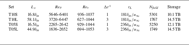
 Lx
 Reθ
 θ
 Reτ
 Δt+
 Reτ≈1000
 tL
 δin
 u∞
 Nfield
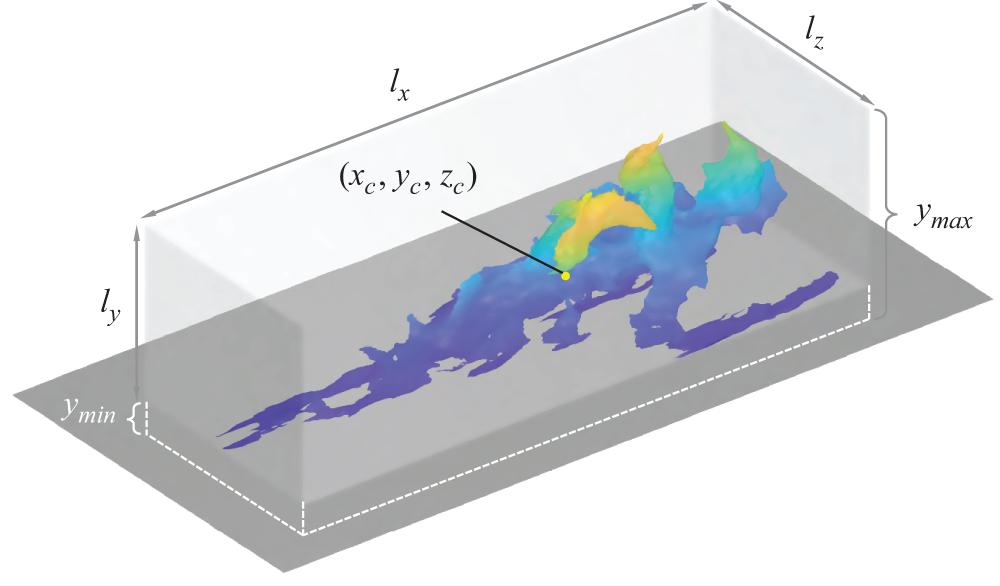
 u′
 lx
 ly
 lz
 (xc,yc,zc)
 ymax
 ymin
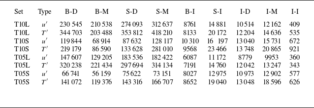
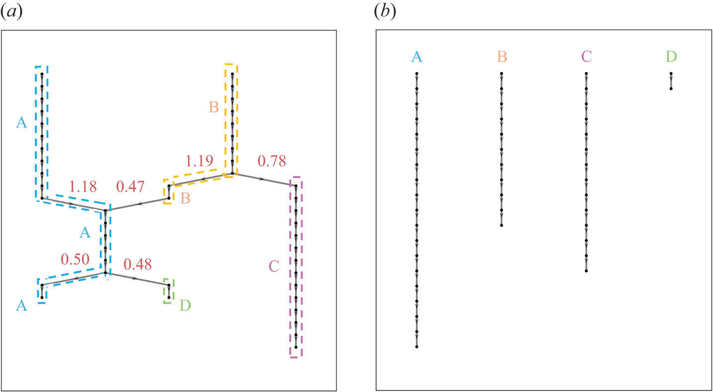
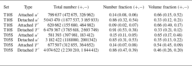
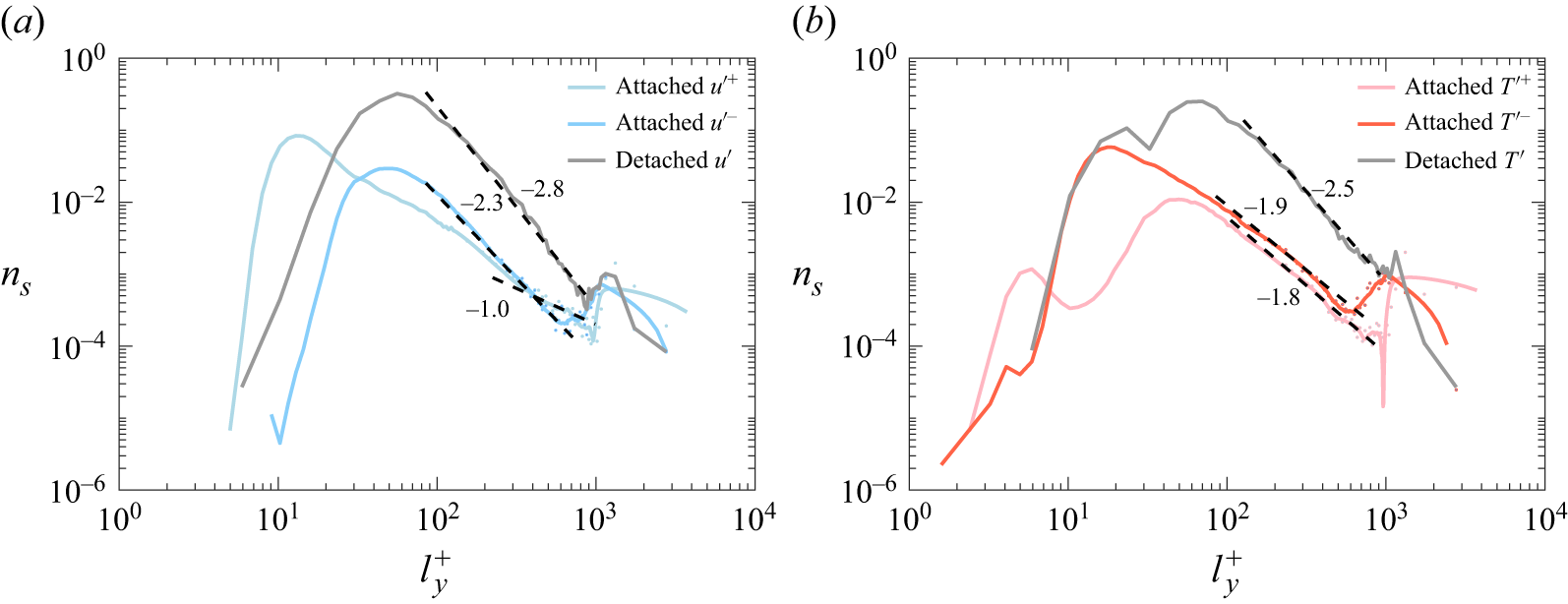
 u′
 T′
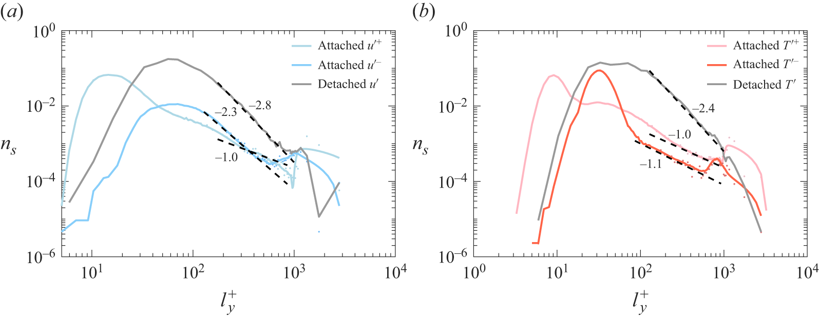
 u′
 T′
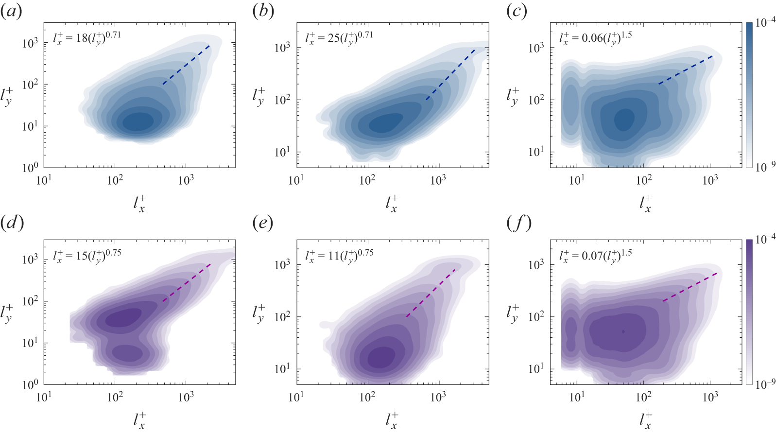
 u′
 T′
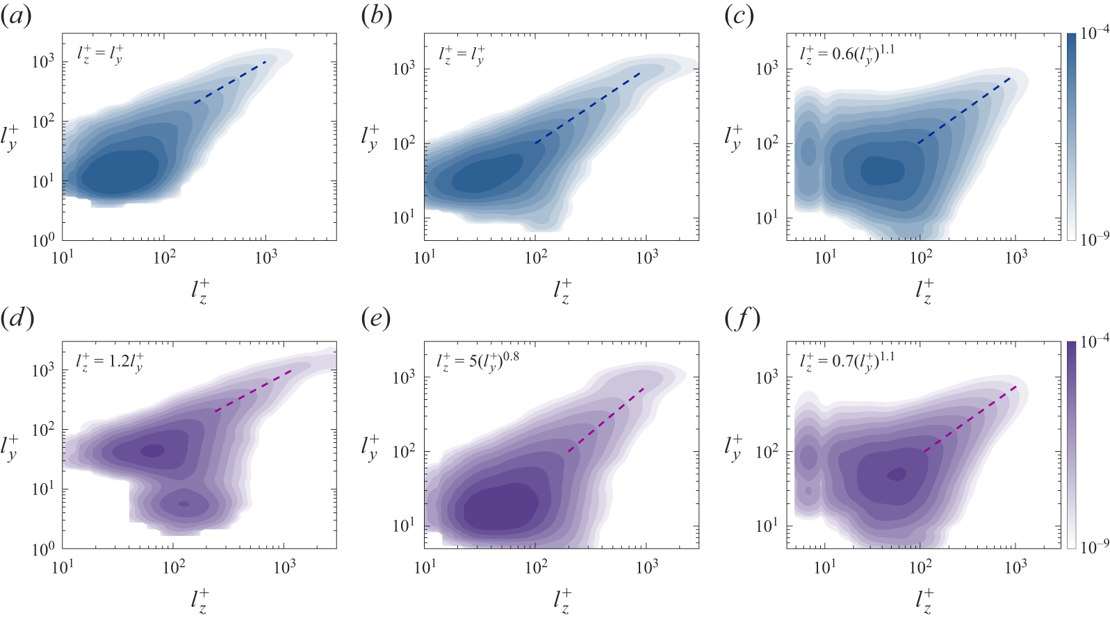
 u′
 T′
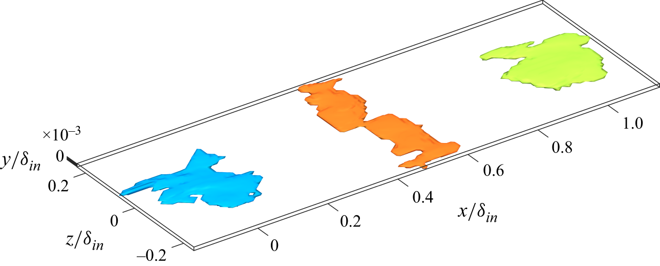
 T′+
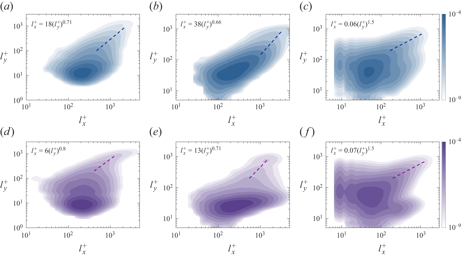
 u′
 T′
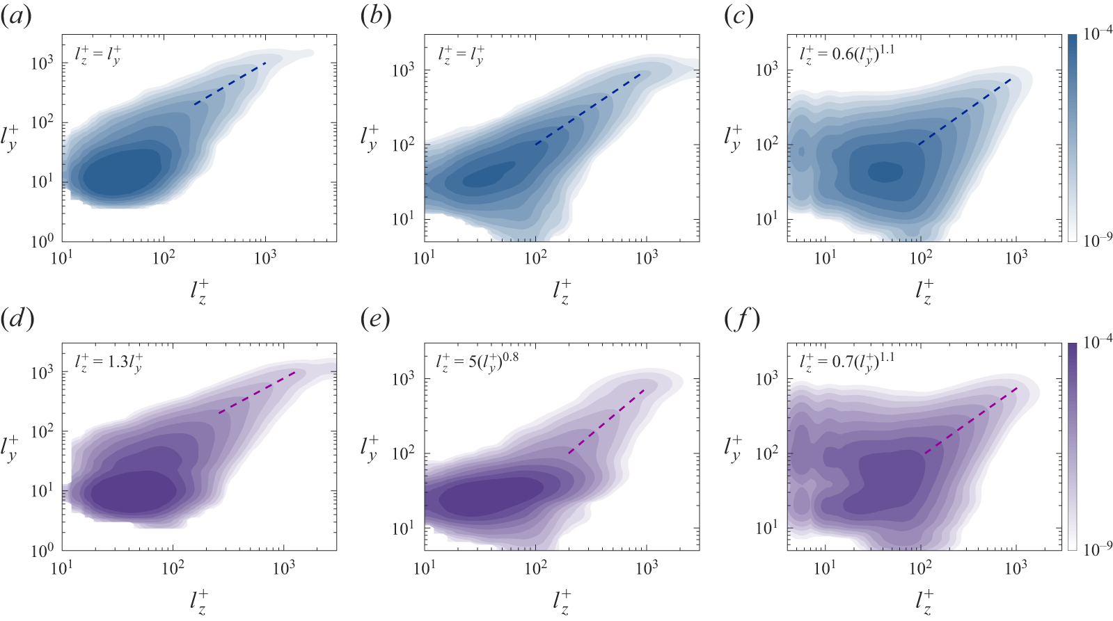
 u′
 T′

 u′−
 u′
 T′
 u′
 T′
 u′
 T′

 p(Uadv|yc)
 u′+
 u′−
 T′+
 T′−
 u¯
 Reτ=985

 p(Uadv|yc)
 u′+
 u′−
 T′+
 T′−
 u¯
 Reτ=985
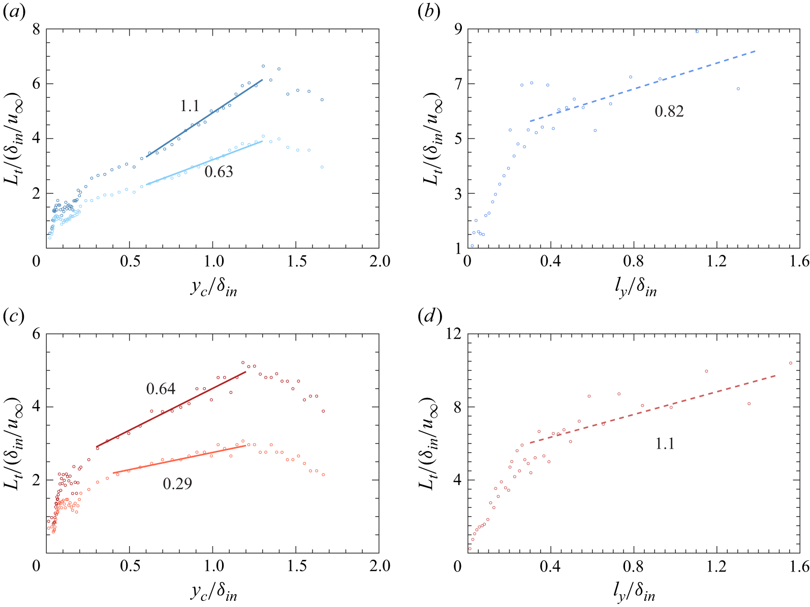
 Lt
 u′
 u′
 T′
 T′
 yc/δin<0.2
 yc/δin>0.2
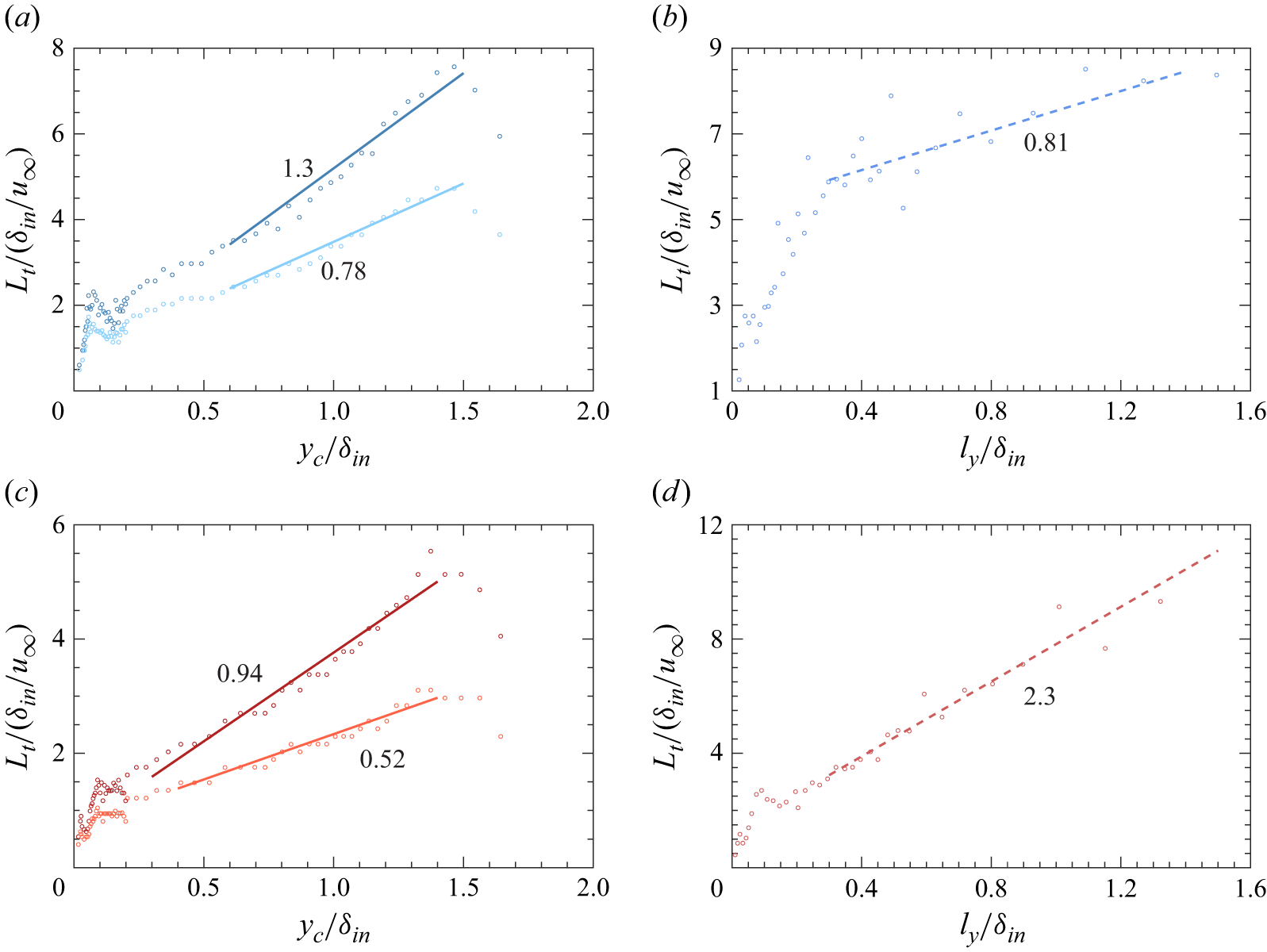
 Lt
 u′
 u′
 T′
 T′
 yc/δin<0.2
 yc/δin>0.2
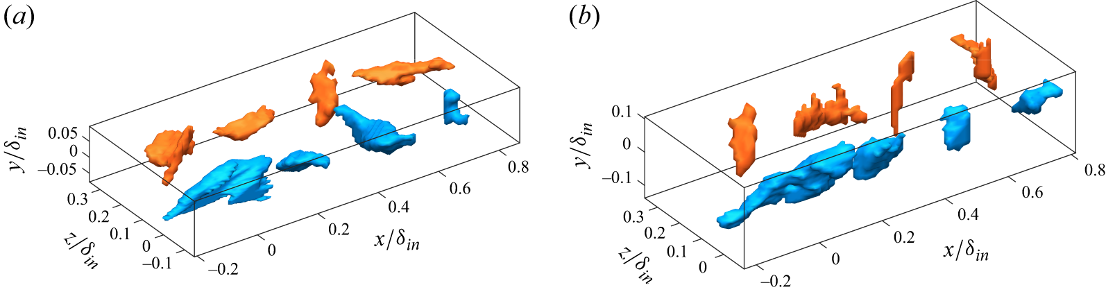
 u′
 T′
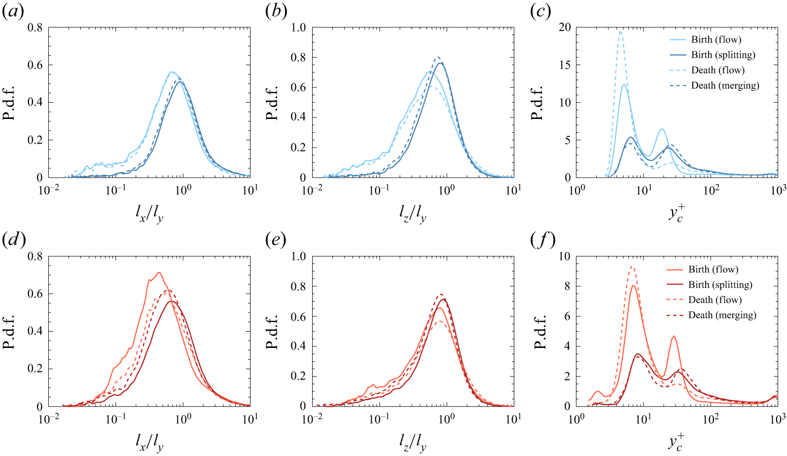
 u′
 T′
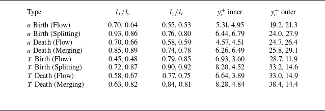
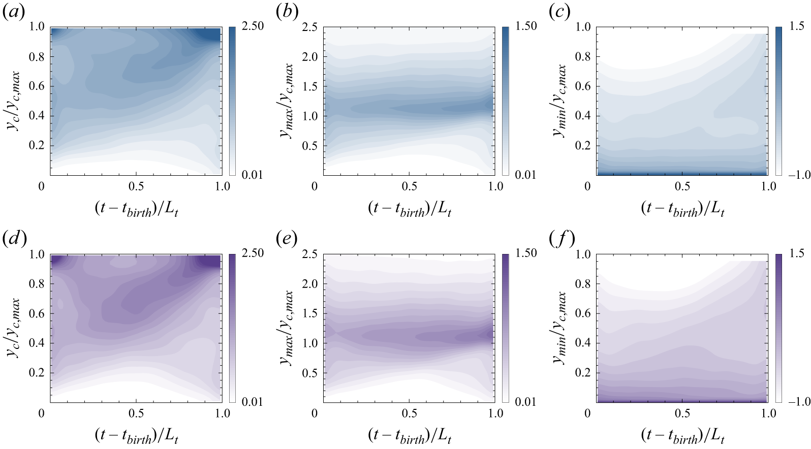
 u′
 T′
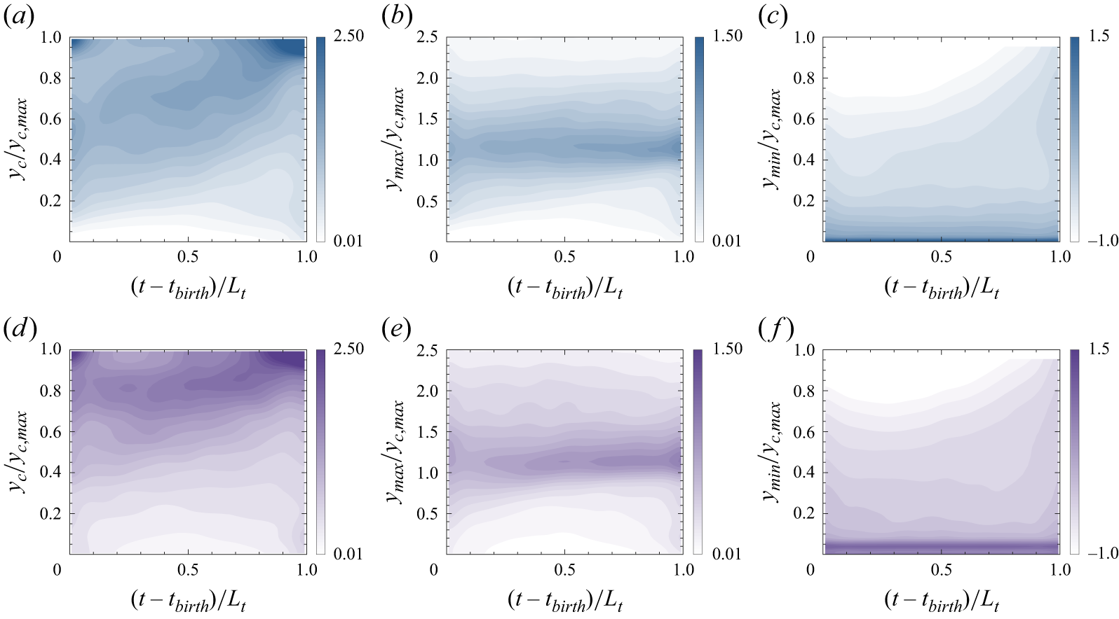
 u′
 T′

 u′
 T′

 u′
 T′
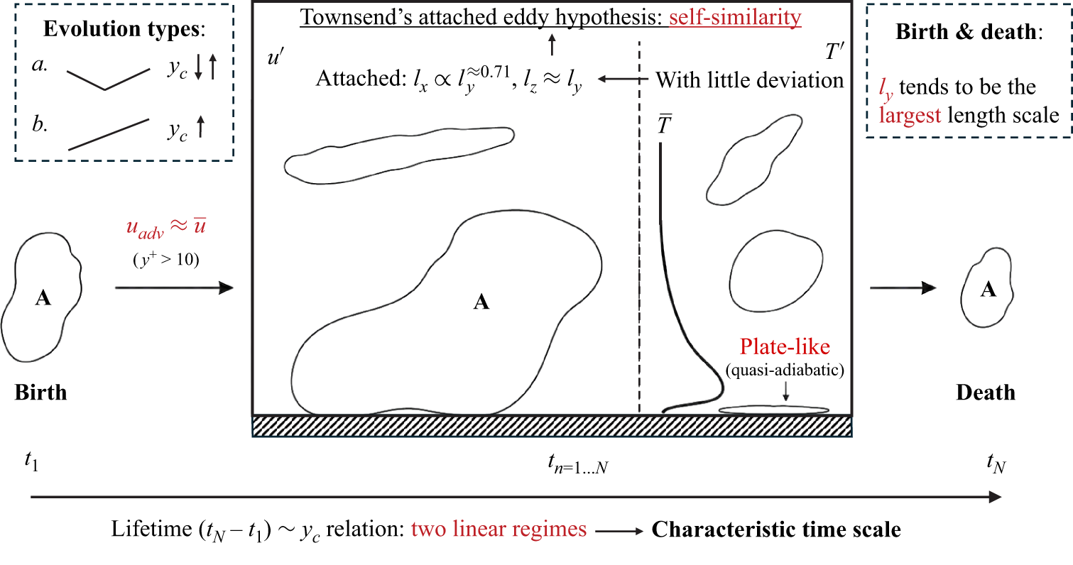
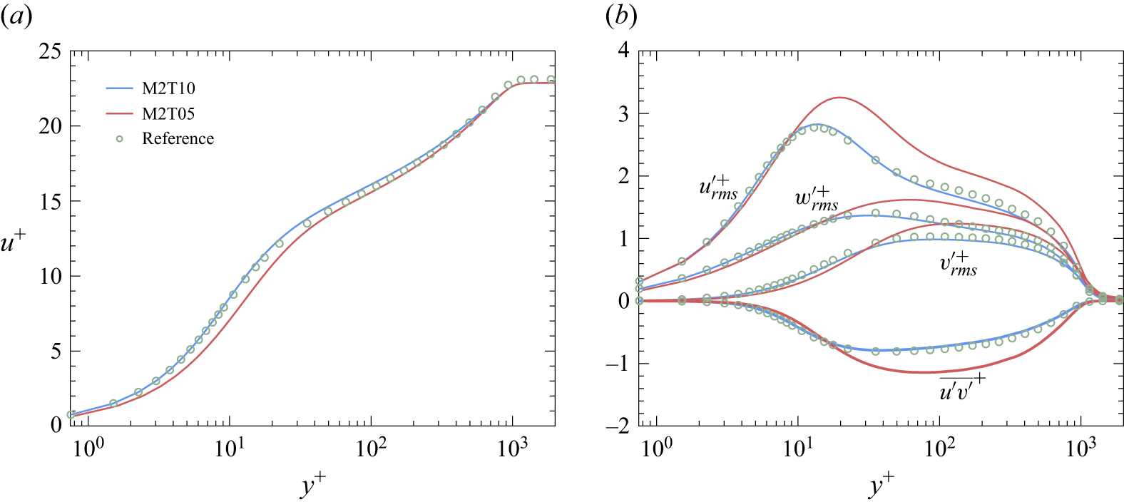
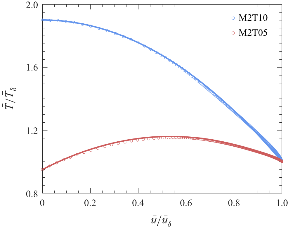

 δ99
 k¯
 ϕ¯
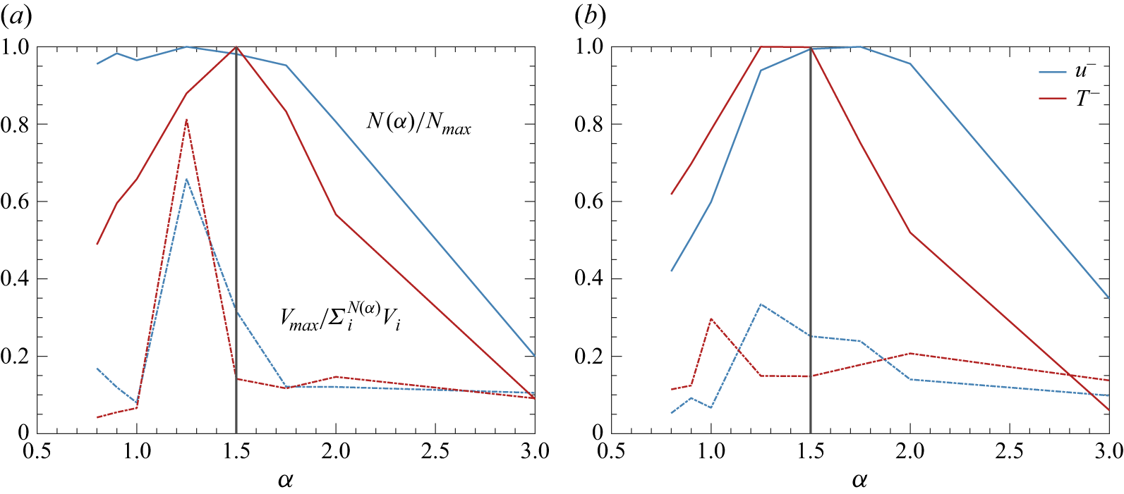
 N(α)
 α
 Nmax
 α
 V
 Vmax
 α


