II. GROUND-BASED MEASUREMENT OF SCATTERING COEFFICIENT

The radar backscattered ground return is measured with a scattering coefficient σ⁰, which is the ground cross-section per surface unit area. The parameter is by definition independent of the measurement system, but varies with the used electromagnetic wave features such as wavelength, polarization, incidence angle as well as with the reflecting surface type.

In the simplest case, it can be assumed that the coefficient is constant within the antenna footprint. Indeed, it is true if the beamwidth is small and observed surface is homogeneous. The expression for its value can be derived from radar equation [Reference Moore5] it takes form of (1), where P _r and P _t are the received and transmitted powers, respectively, λ is the wavelength, G _Tx and G _Rx are the transmitting and receiving antenna gains, R is the distance in sounding direction and A is the illuminated ground surface element.

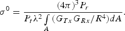(1)$$\sigma ^0={\lpar 4\pi \rpar ^3 P_r \over {P_t \lambda ^2 \vint\limits_A \, \lpar G_{Tx} G_{Rx} /R^4 \rpar dA}}.$$

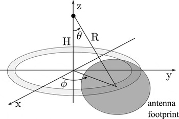
A small footprint in the L-band that would cover uniform surface and small extent of incidence angle requires large aperture dimensions. Such antennas could not be mounted on a transportable and easily-set mast. On the other hand, the result of radiometric measurement conducted with wide-beam antennas integrates different incidence angles and surface types. This would not provide the desired information about the surface characteristics. The solution, however, is to use a radar system that associates the incoming echo power level with its delay and thereby the range. In such a case, each cell of a range profile covers backscattered ground echo from a ring of the land (Fig. 1). Moreover, the range compression that is performed in a radar system may improve the dynamics and add statistically independent profile samples.

Fig. 1.

Scene geometry.

Now, equation (1) can be transformed to that case. The area element in integration for geometry depicted in Fig. 1 can be expressed as:

(2)$$dA=R^2 \sin\!\lpar \theta \rpar \cos\!\lpar \theta \rpar d\theta d\phi .$$

After simple transformations, the exact expression for the scattering coefficient of a ring of the examined surface takes the following form:

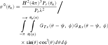(3)$$\eqalign{\sigma ^0 \lpar \theta _n \rpar &={H^2 \lpar 4\pi \rpar ^3 P_r \lpar \theta _n \rpar \over P_t \lambda ^2} \bigg{/} \cr & \quad \vint\limits_{ - \pi }^{ - \pi } \, \vint\limits_{\theta _l \lpar n\rpar }^{\theta _u \lpar n\rpar } \, G_{Tx} \lpar \theta - \psi\comma \; \phi \rpar G_{Rx} \lpar \theta - \psi\comma \; \phi \rpar \cr & \quad \times \sin\! \lpar \theta \rpar \cos ^3\! \lpar \theta \rpar d\theta d\phi }$$

where H is the antenna mast height, P _r(θ_n) is the power return for the nth range profile's cell, ψ is the antenna pointing direction, θ_n is the incidence angle for the middle of the nth range cell projected onto the ground, while the integration limits θ_u(n) and θ_l(n) determine the ring corresponding to the cell. The integration is done over a much smaller area than in the full-beam approach and it is more likely that the land cover within it will be uniform, which makes the interpretation of the result much easier.

As can be deduced from equation (3), in order to calculate the σ⁰ coefficient not only the profile value but also two other factors are needed – antennas radiation patterns and the transmitted power level value including all signal losses and gains of the system. The issues of calibration will be described in Section IV of the paper.

III. RADAR SYSTEM SETUP AND SIGNAL PROCESSING

A) Hardware setup

Development of a full radar system dedicated to a purely scientific, specific purpose can hardly find an economical justification. Owing to that a concept of a software-defined radar demonstrator built from commercial-off-the-shelf (COTS) elements was utilized [Reference Maslikowski, Contartese, Malanowski and Kulpa6]. As the sounding waveform a pseudo-noise signal was chosen.

The bases of the system are a three-channel vector signal analyzer (NI PXIe-5663) working as the receiver, and an arbitrary waveform generator (AWG) (Agilent MXG N5182A), which was used as the source of the illuminating signal. The AWG synthesizes a baseband signal according to digital samples from its memory and upconverts it to the desired frequency band. The analyzer conditions, downconverts and digitizes the waveform. All of the three channels are synchronized and phase coherent.

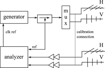
Since the radar system is required to acquire polarimetric range profiles of the ground surface, two transmitting and two receiving log-periodic antennas of each polarization (H and V) were used. In the paper, vertical polarization V is assumed to be the one acquired with antenna dipoles directed vertically. The antennas were mounted on a 12 m high mast. During the first part of the signal acquisition, the transmitting antenna with horizontally directed dipoles was active and two receiving ones with both polarizations collected the scene echoes. The signals were recorded on two channels of the analyzer, while the third was employed to capture the reference waveform needed for range compression. After that, the second transmitting antenna was activated using an RF multiplexer and the recording was repeated for vertically polarized excitation. The diagram of the system is presented in Fig. 2. The power transmitted from the generator was equal to 26 dBm but due to the cable losses, RF low-noise amplifiers had to be used on the receive site in order to maintain high signal-to-noise ratio (SNR).

Fig. 2.

The radar demonstrator system setup.

The analyzer's bandwidth is limited to 50 MHz which gives approximately 3 m of range resolution. To cover a wider bandwidth, stepped-frequency operation mode was utilized. The observations were performed at seven neighboring sub-bands, starting with 1.05 GHz of centre frequency, which makes up 350 MHz of bandwidth centered around 1.2 GHz. This enables wideband signal spectrum synthesis and generation of a high resolution range profile [Reference Maslikowski and Malanowski7]. Here, unlike in the case of imaging radars, it was not necessary and additional data from sub-bands were used in incoherent averaging. Owing to the fact that profiles from different bands are statistically independent, it decreased the variance of the resultant standard-resolution profile.

B) Noise radar signal processing

A range profile in a software-defined noise radar is the cross-correlation between the reference and surveillance signals, which correspond to the matched filtering in a classical radar [Reference Lukin8]. Like in a classical linear frequency modulation (LFM)-based radar, any distortion in the channel frequency response results in significant sidelobes in the compressed profile domain. To deal with that, an inverse filter based on digital waveform from AWG (Arbitrary waveform Generator) memory and a measurement in the calibration setup (with cable connections instead of antennas – see Fig. 2) was developed. Based on that, the equalization of the measurement system frequency characteristics was applied to the measured cross-spectra. In such a case, a reference oscillator relative drift drastically degrades the performance. To mitigate that effect the synchronization between the analyzer and the generator was locked and drifts did not affect the equalization quality.

Another significant problem in a continuous wave (CW) radar is the direct path signal between the Tx and Rx antennas as well as the strong echo from nearby ground surface. The interference not only consumes the vertical range of the measurement system but also introduces correlation sidelobes and residual fluctuations [Reference Axelsson9] that mask weaker echoes, and in the case of scatterometry, may deform the shape of a ground profile. In order to be sure that the measured profile is not the sidelobe of the correlation peak but real value of the backscattered power, the profile was merged from two parts. One, covering the direct leakage and strong echoes from small distance, was computed conventionally as a cross-correlation between the reference and unfiltered surveillance signal. The second, covering weak echoes from distant range cells, was calculated using a lattice filter that removed strong echoes with all their artifacts from the surveillance signal [Reference Kulpa and Czekala10].

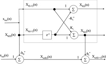
The filter structure is presented in Fig. 3, where K _i and h _i coefficients are described with:

Fig. 3.

A diagram of the lattice filter for clutter removal.

(4)$$K_i=\displaystyle{{2\sum\nolimits_{n=i+1}^N \, x_{b\lpar i - 1\rpar } \lpar n - 1\rpar x_{f\lpar i - 1\rpar }^ {\ast} \lpar n\rpar } \over {\sum\nolimits_{n=i+1}^N \, \vert x_{b\lpar i - 1\rpar } \lpar n - 1\rpar \vert ^2+\vert x_{f\lpar i - 1\rpar }^ {\ast} \lpar n\rpar \vert ^2 }}$$

and

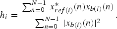(5)$$h_i=\displaystyle{{\sum\nolimits_{n=0}^{N - 1} \, x_{ref\lpar i\rpar }^ {\ast} \lpar n\rpar x_{b\lpar i\rpar } \lpar n\rpar } \over {\sum\nolimits_{n=0}^{N - 1} \, \vert x_{b\lpar i\rpar } \lpar n\rpar \vert ^2 }}.$$

The idea behind is that the received signal can be decomposed into two subspaces: clutter subspace and useful echoes subspace. The clutter subspace bases on delayed copies of the reference signal. Unfortunately, they do not constitute a fully orthogonal base so that projection of the received signal onto the clutter subspace needs prior orthogonalization. A widely known method is for example the Gram–Schmidt algorithm, but it is computationally expensive. A much more effective algorithm is based on a lattice prediction filter [Reference Friedlander11, Reference Haykin12] that produces a set of orthogonal vectors at its output (Fig. 3).

With orthogonal base vectors of the clutter subspace the projection of the received signal on that set can be easily done. Then, by subtracting the projection from the received signal one can obtain its clutter-free version.

As can be observed in Fig. 4, between the beginning of the filtered profile and the range of 200 m the profiles are convergent. Also, significant decrease (10 dB) in the residual fluctuations level can be seen. However, since the mast height is 12 m, it corresponds to a nearly horizontal incidence angle so that the filtering is not necessary in the measurement of the scattering coefficient as a function of the incidence angle. The main advantage of filtering here is that it proves that the profiles are not distorted by the system's dynamic range.

Fig. 4.

The result of strong echoes cancellation on measured range profiles.

IV. CALIBRATION ISSUES

As was mentioned in Section II, the antenna gain patterns and power balance must be known in order to calculate the value of the scattering coefficient σ⁰. A common practice is to use a standard target of known radar cross-section (RCS), such as a corner reflector [Reference Chet, Kuan and Teik13, Reference Strozzi, Matzler and Weise14]. In this study, however, another approach was chosen due to the fact that the authors did not use the antenna rotator.

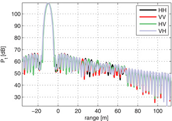
In order to measure the transmitted power P _t, a calibration setup was chosen with a connection between Tx and Rx cable ends instead of the antennas. The measurement takes into account the transmitted power level, cable losses, and amplifiers gains. What is necessary is to use an attenuator in order not to saturate the receiver. In the described case, as much as 30 dB of attenuation and decrease in the transmitted power level of 25 dB was needed. The calibration profiles that in fact represent the point spread function of the radar system (without the antenna influence) are depicted in Fig. 5. Since the range compression is performed for regular scene sounding, the result is automatically scaled in the same way as the scene ground profile. The maximum of the calibration profile is the searched value of P _t. The absolute value of the transmitted power does not have to be known. What is important is the ratio between P _r(θ_n) and P _t. Of course, the method is prone to any mechanical changes that may occur during cable switching.

Fig. 5.

Calibration profiles.

The antennas gain pattern can be naturally measured in an anechoic chamber, however for the L-band it would require large size of the absorbing elements and the chamber itself. Another solution is to use an electromagnetic simulator to determine the shape of the beam. Since those are not the concerns of the current paper, a simpler approach was chosen that will provide some approximate solution. When a log-periodic antenna operates in an appropriately narrow band, it can be assumed that only three elements are in the active region of the antenna. Simplifying the matter more, the antenna was treated as a three-element Yagi-Uda array. Expression and scripts for the antenna gain and radiation pattern for such a case can be found in [Reference Orfanidis15].

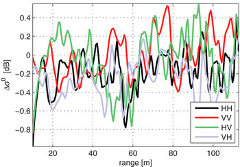
For antennas with horizontally directed dipoles, the variables θ and ϕ in expressions for patterns were swapped in comparison with a vertically directed dipole since the same antennas were used for both polarizations. Then, the scattering coefficient was calculated for six different antenna inclinations angles between 45° and 80°. The error between σ⁰ for extreme inclinations was plotted in Fig. 6. As can be seen, a small bias and minor trend caused by miscalibration lies within the profile fluctuations and can be neglected. Measurements carried out for different antenna inclination angles give one more advantage. Since the antenna phase center changes its position, the results obtained for different antenna slants are statistically independent and can be effectively used for averaging.

Fig. 6.

Antenna gain calibration error between measurements with θ₀ = 45° and θ₀ = 80°

V. MEASUREMENT CAMPAIGN AND ITS RESULTS

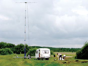
The latest outdoor measurement campaign was carried out in July 2012 at three points in the Biebrza river valley: meadow and reeds in Kopytkowo village (53°35′17″N, 22°53′39″E), area of marshy sedge meadows in the Biebrzanski National Park near Ciszewo village (53°37′14″N, 22°42′07″E), and cultivated meadows near Biebrza village (53°39′42″N, 22°37′05″E). Each point was characterized by different vegetation structure and soil moisture. The measurement hardware was situated in a camping trailer and the 12 meter-high antenna mast was directed toward the observed meadow surface. The points were chosen so that the beam illuminated possibly homogeneous plant communities. The trailer and the mast situated on a measurement site are presented in Fig. 7.

Fig. 7.

Antenna mast and the trailer on a measurement site.

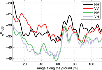
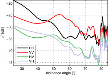
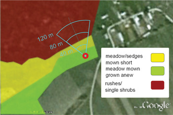
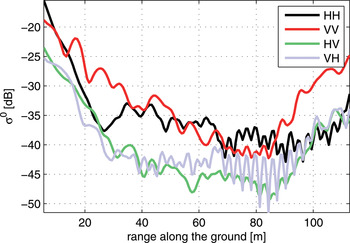
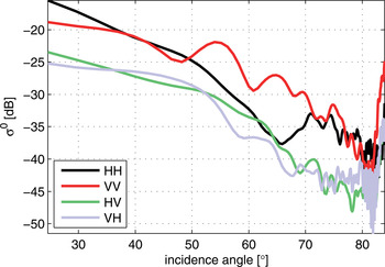
For each antenna position the measurement was repeated five times on all seven sub-bands. The results were then averaged over sub-bands and oversampled by a factor of 5 to smoothen the plots. An exemplary result of the measured scattering coefficient in Kopytkowo village σ⁰ is presented in the Fig. 8 as a function of the distance along the ground, and in Fig. 9 as a function of the incidence angle θ. At a distance of 60 m a sudden growth in the coefficient values can be observed. Indeed, a field of rushes and single shrubs began there. A schematic map presenting land cover and 60° antenna footprint can be seen in Fig. 10.

Fig. 8.

Ground scattering coefficient σ⁰ measured in Kopytkowo as a function of the distance along the ground.

Fig. 9.

Ground scattering coefficient σ⁰ measured in Kopytkowo as a function of the wave incidence angle θ.

Fig. 10.

Schematic map of the observed plant communities in Kopytkowo.

On the other measurement spot, in the marshy meadows area near Ciszewo, the radar system was directed towardnearly uniform meadow limited with an edge of a forest. It can be seen that the reflectivity reaches the threshold of system sensitivity near the 80th meter (Fig. 11). Owing to a more uniform land cover, the descent in the incidence angle domain, especially for VV polarization, is much more monotonous than on the previous spot (Fig. 12). Over the 80th meter the verge of the antenna beam spans over the forest and the measured coefficient rapidly grows. Although the results seem reasonable, they cannot be treated as reliable as long as they are not verified with measured antenna pattern.

Fig. 11.

Ground scattering coefficient σ⁰ measured on the Ciszewo site as a function of the distance along the ground.

Fig. 12.

Ground scattering coefficient σ⁰ measured on the Ciszewo site as a function of the wave incidence angle θ.