Introduction
Centile charts for body weight (BW) and height are routinely used to track the normal growth and development of children alongside their birth percentile, allowing their health and progress to be monitored. Poor weight gain and slow growth have been linked to cot death (Sinclair-Smith et al., Reference Sinclair-Smith, Dinsdale and Emery1976), developmental delay (Dowdney et al., Reference Dowdney, Skuse, Heptinstall, Puckering and Zur-Szpiro1987), ischaemic heart disease (Barker et al., Reference Barker, Osmond, Winter, Margetts and Simmonds1989), non-insulin-dependent diabetes and hypercholesterolaemia (Barker, Reference Barker1995a and Reference Barker1995b). The Developmental Origins of Adult Disease (DOAD) hypothesis proposes that pre- and postnatal growth and development influence health in later life (Barker, Reference Barker2004).
For many years children have been measured and compared with standard height and weight curves. Whilst these may give some indication of growth and development, they are a poor predictor of body shape. The power function of weight/heightn is a good measure of whether a person is overweight (Wright et al., Reference Wright, Matthews, Waterston and Aynsley-Green1994); n is usually a whole number, n = 2 gives a measure called the body mass index (BMI) (Cole, Reference Cole1995) and n = 3 ponderal index (PI) (Eriksson et al., Reference Eriksson, Forsen, Tuomilehto, Osmond and Barker2001). BMI is a measurement of a combination of height, weight, body fat and muscle, which, although a less straightforward measure of growth than height, is a far better indicator (Wright et al., Reference Wright, Matthews, Waterston and Aynsley-Green1994). PI is somewhat comparable to BMI, but gives a fairer comparison between individuals of different stature. PI in newborn infants has been used as an indicator of foetal growth status, especially to assess asymmetrical intrauterine growth restriction. More recently, PI (weight/height3), a three-dimensional measurement accounting for BW and shape, has been shown to be an important indicator of future health (Barker, Reference Barker1998). For example, death from coronary heart disease was associated more strongly with a low PI than low birth weight at birth (Forsen et al., Reference Forsen, Eriksson, Tuomilehto, Teramo, Osmond and Barker1997). Low weight and thinness at birth (i.e. low PI) may also increase the risk of developing insulin resistance in later life (Phillips et al., Reference Phillips, Barker, Hales, Hirst and Osmond1994).
Many children deviate from their early percentile, but it is still not clear as to when the point at which they deviate becomes of pathological importance (Wright et al., Reference Wright, Matthews, Waterston and Aynsley-Green1994). There is a growing body of evidence to suggest that postnatal ‘catch-up’ or ‘catch-down’ growth may also be a contributory factor to predisposition to adulthood diseases (Roolan-Cachera et al., Reference Roolan-Cachera, Deheeger, Akrout and Bellisle1995; Ong et al., Reference Ong, Ahmed, Emmett, Preece and Dunger2000, Reference Ong, Preece, Emmett, Ahmed and Dunger2002 and Reference Ong, Petry, Emmett, Sandhu, Kiess, Hales, Ness and Dunger2004; Koletzko, 2006). Such children had greater BMI, % body fat, total fat mass and central fat distribution, which are variables of childhood size linked to metabolic markers for risk of disease in adulthood (Vanhala et al., Reference Vanhala, Vanhala, Kumpusalo, Hadonen and Takala1998) and are predictive for adulthood obesity (Simmons and Breier, Reference Simmons and Breier2002). To more accurately monitor growth, BW can be transformed to standard deviation (s.d.; or Z) scores, which allow the latest s.d. score to be compared with the baseline (birth) s.d. score (Wright et al., Reference Wright, Matthews, Waterston and Aynsley-Green1994). A gain in s.d. score for weight over a given time frame that was greater than 0.67 s.d. scores is taken to indicate clinically significant catch-up growth, as 0.67 s.d. scores represent the width of each percentile band on standard growth charts that is, second to ninth percentile, ninth to 25th, 25th to 50th, and so on. Similarly, a decrease in s.d. scores for weight by more than 0.67 s.d. scores indicated catch-down growth.
Whilst percentile curves for growth and development are useful for identifying infants at risk, ethical considerations mean that it is not possible to manipulate environmental and physiological factors in an attempt to mitigate the risk. Consequently, various animal models have been used to study the DOAD hypothesis. The pig is a species that is considered to be biologically similar to humans in terms of metabolism (Cooper, Reference Cooper1975), and is widely used in biomedical research, particularly in the fields of cardiovascular disease and diabetes. The natural variation in BW and shape at birth make it an ideal model for studying the underlying mechanisms for foetal programming, and the subsequent relationships with postnatal growth and predisposition to adulthood diseases.
In the past, piglet weights have been plotted against a cumulative sample proportion on a normal probability scale (Walker and Lev, Reference Walker and Lev1969). The construction of percentile curves for pigs, similar to those used for human studies, would allow an efficient method of following an individual pig’s growth, particularly during experimental manipulations. For example, both nutrition and the environment have extensively been shown to have a pronounced influence on porcine growth curves (Widdowson and McCance, Reference Widdowson and McCance1975). Such curves could be used to distinguish if a pig deviates from its early percentile curve, and identify when, or if, the point at which they deviate becomes of pathological importance. Whilst it is noted that humans were measured using height, crown-to-rump length (CRL) is the most appropriate representation of height in the pig. The aim of the study was to construct percentile growth charts for BW (from birth to 160 days) and PI (from birth to 1 month of age) to enable the monitoring of the growth of individuals used in biomedical research.
Materials and method
Animals and nutrition
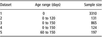
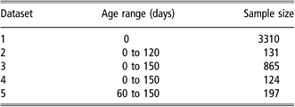
Data comprise five data sets (Table 1) collected from a commercial (Landrace × Large White) herd maintained at the Pig Research and Development Unit, Imperial College London, between 2000 and 2004. As with the human growth data sets used by Cole (Reference Cole1995), data were collected over several years, and at different time of the year, to give a true representation of the whole population growth and development. The floor space for pigs, at all stages of life, was in excess of the current codes of recommendations for the welfare of pigs published by the Department for Environment, Food and Rural Affairs (DEFRA). Ambient temperature was maintained within the recommended range (DEFRA, 2003) by altering the ventilation rate. Heat lamps were provided in the creep area for piglets to reduce the risk of hypothermia.
Summary of age range and sample size of piglets in each dataset
Sows were housed in straw yards and offered 3 kg/day of standard diet (ABN HE sow pellets; 13.1 MJ/kg; 1.7% protein; 4.5% fat; ABN, Peterborough, UK). Sows were placed in specialised farrowing accommodation prior to natural farrowing at term and were offered 6 to 9 kg/day lactation pellets (ABN Supreme lactation pellets; 14.1 MJ/kg; 18% protein; 7.2% fat; ABN) during lactation. Male piglets were not castrated and all piglets were sow reared until weaning occurred at 26 and 28 days, providing they weighed >6 kg. Any piglet not reaching this BW was crossed-fostered onto another sow until they reached the desired weight. As weaning is a stressful process, only a small subset of pigs on the longitudinal studies was weighed on day 30. After weaning, piglets were housed in single-sex groups and offered ad libitum a commercially available diet, appropriate for BW and stage of development (ABN), until they were humanely slaughtered for meat purposes.
Piglet BW, CRL and limb length were recorded within 24 h of birth and weekly thereafter until weaning occurred. After weaning, BW was recorded at 60, 90, 120 and 150 days of age. PI was calculated from measurements taken at 0, 7, 14 and 21 days of age using the formula PI = weight/CRL3. It is noteworthy that piglet mortality rates on the commercial unit were typically between 3% and 8%, and so not all piglets recruited onto the study survived to day 150. Similarly, for human studies not all data would have been collected for each infant due to mortality, morbidity or failure to record measurements for other reasons.
Data set 1 is cross-sectional, with measurements being recorded within the first 24 h of life (Table 1), whereas the other data sets (2–5) are longitudinal; piglets were followed and measurements were taken at different stages of the pig’s life from 0 to 150 days of age. Data set 2 only follows pigs to 120 days as these met the criteria for the bacon market, but during the time course of data collection, there was a change in market forces and animals were sent for slaughter at a heavier weight, and hence age.
Initially these data were separated by sex and all analyses were carried out for each of the sexes separately. Both groups were subsequently subdivided into the following age categories: birth, 7, 14, 21, 30, 60, 90, 120 and 150 days for BW, and birth, 7, 14 and 21 days of age for PI. Data were analysed using Cole’s lambda-mu-sigma (LMS) method (Freeman et al., Reference Freeman, Cole, Chinn, Jones, White and Preece1995). As the physical measurements taken were non-normal in distribution (as is the case for most physical measurements (Wei and He, Reference Wei and He2006)), the data at each age and for each sex were transformed to normality using a Box–Cox power transformation. The Box–Cox transformation is the most widely used method in this respect, and the LMS method is the most sophisticated (Wei and He, Reference Wei and He2006). The centiles for each age and sex were summarised in terms of the Box–Cox power needed to make the distribution normal. This fitting process ensured that the values of L, M and S changed smoothly with age so that they could be represented as smooth curves plotted against age. These three parameters provided the required centiles using the following equation (Cole, Reference Cole1995):

where C 100α(t) is the centile curve plotted against age t, L(t) is the best-fitting Box–Cox power for the transformed variable Y(t), M is the median of Y(t), S(t) is the scale of Y(t) and zα is the normal equivalent deviate for the centile. For example, when α = 0.97 corresponding to the 97th centile, zα = 1.88; likewise, when α = 0.9, 0.75, 0.5, 0.25, 0.1 or 0.03, then zα = 1.28, 0.67, 0, −0.67, −1.28 or −1.88, respectively. As quoted by Freeman et al. (Reference Freeman, Cole, Chinn, Jones, White and Preece1995), the main advantages of this approach are as follows: (i) it estimates the extreme centiles more efficiently than the simpler sort and count procedure, while accounting for skewness in the distribution; (ii) it can generate any required centiles, not just the conventional ones; and (iii) centiles constructed by the LMS method assumes that at a given time point t, the measurement Y(t) can be transformed to be approximately standard normal by the data to be transformed directly to s.d. or Z scores (Z(t)) using the following equation:

where Y is the pig’s measurement (weight or PI), and L(t), M(t) and S(t) are values read from the smooth curves for the pigs’ age and sex.
Results
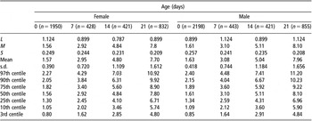
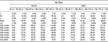
Tables 2 and 3 show the weight centile curves, using seven centiles (3, 10, 25, 50, 75, 90 and 97), for female and male pigs from birth to 21 days of age, and from day 30 to day 150 of life, respectively.
Body weight percentile data for female and male pigs during the neonatal period

L = lambda, for the skew; M = mu for the median; and S = sigma for the generalised coefficient of variation.
Body weight percentile data for female and male pigs during the post-weaning phase (30 to 150 days of age)

L = lambda, for the skew; M = mu for the median; and S = sigma for the generalised coefficient of variation.
During the neonatal period, weight centile curve patterns are similar between both female and male animals; all the centiles are close together and rising. Around weaning, a fall in weight can be seen in both the male and female groups. After a post-weaning adaptation period, all the female centile curves continue in a similar pattern until the final measurement at 150 days of age. In contrast, the male centile curves only follow a similar pattern of growth to 120 days of age, after which those in the lower centiles (3rd and 10th, and to a lesser degree 25th) lose weight; this is the age at which most contemporary breeds reach puberty (Bazer et al., Reference Bazer, Ford and Kensinger2001). By the time the final recording is taken at 150 days of age, growth rate appears to have ‘re-stabilised’. It is of interest to note that the BW of male and female pigs for each percentile is comparable during the neonatal period and the post-weaning phase, with the exception of the 3rd centile at 150 days when female pigs are approximately 6 kg lighter than their male counterparts.
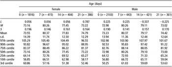
Table 4 shows the PI curves over the neonatal period from birth to 21 days (i.e. prior to weaning) of age using the same seven centiles as described above for BW. As previously mentioned, PI is a measure of body conformation; piglets with a low PI are long and thin, whereas piglets with a high PI are short and fat. Percentile curves for female piglets showed an increase in PI between day 0 and day 7 in all but the fattest pigs (90th and 97th centiles). After day 7, PI declined gradually at all subsequent time points. In the male pigs, those with a PI lower than the 50th centile (i.e. the longer, thinner pigs) followed the same pattern as the female pigs with PI increasing until day 7 and declining thereafter. Pigs in the upper percentiles continued to get fatter until day 14, after which the PI began to decline.
Ponderal index (kg/m3) percentile data for female and male pigs from birth to 21 days of age

L = lambda, for the skew; M = mu for the median; and S = sigma for the generalised coefficient of variation.
Discussion
Growth charts or reference centile charts for humans have been widely used to determine the growth of an individual within the context of population values; we have for the first time constructed BW and PI reference centiles for pigs, a valued biomedical model for human medicine. It is clear from the percentile charts constructed for pigs that, as in humans, growth charts are an acceptable way of monitoring growth and development of individuals. Weight percentile curve patterns are similar between both females and males; all the centiles are close together and continue to rise during the neonatal period. In the human, weight-for-age continues to increase from birth until after puberty; similarly in the pig, weight-for-age increases until slaughter at around 4 to 5 months of age.
The differences between the pig and human curves can be explained by management practices. The dip in the percentile weight curve of the pig at day 30 occurs as a result of weaning. Naturally, in sows, as in other mammals, milk yield is dependent on the stage of lactation. Milk yield is generally low during the first week of lactation, it rises until it reaches it peak at approximately 3 weeks and remains fairly constant until the 6th week of lactation, after which it begins to decline (Allen and Lasley, Reference Allen and Lasley1960). In the commercial situation, piglets are weaned by removing them from the sow at about 24 to 28 days of age. Weaning is a stressful time for the piglet because of a sudden change in diet from milk to creep feed and the necessity to establish a new dominance hierarchy. The increased stress and reduced energy intake at this time cause a growth check or period of weight loss (Whittemore, Reference Whittemore1993). Allowing the sow to wean the piglets naturally would minimise or remove the dip, causing the curve to be more similar to that of the human.
The change in weight gain of male pigs between day 120 and 150 can be explained by the attainment of puberty, which occurs around this time (Lunstra et al., 1986). At puberty, the increased secretion of androgens and oestrogens acts to stimulate growth of the accessory sex glands and activate sexual and aggressive behaviours (Bazer et al., Reference Bazer, Ford and Kensinger2001). Since the pigs were housed in groups, the reduction in growth rate among pigs in the lower percentiles (which are likely to still be prepubertal) may be partly due to their failure to compete for food against the heavier, post-pubertal males. Similar alterations are not seen in the female percentile weight curves as females reach puberty at a later age, around 175 to 210 days (Cede and Bilkei, Reference Cede and Bilkei2004) and because aggressive behaviour does not increase as a result of puberty in the female.
Although PI charts have not been developed for the human neonate, it is used as a cross-sectional growth measurement to assess whether intrauterine growth retardation has occurred. The PI chart for the piglet shows a rise in PI during the first week of life, and a gradual decline thereafter until day 21. The piglet is born with very little fat; in the first week of life the piglet grows very rapidly, and fat deposition increases dramatically. The rate of fat deposition exceeds that of other components (Mitchell et al., Reference Mitchell, Scholz and Mersmann2001) and by the end of the first week of life the piglet may have up to 20 times as much fat as at birth. Consequently, the increase in PI during the first week of life is likely due to the rapid deposition of fat during this period. Likewise, the human neonate grows rapidly and builds up its fat reserves, resulting in a sharp rise in BMI between the 1st and 6th months of life (van’t Hof and Haschke, Reference van’t Hof and Haschke2000). We used PI rather than BMI as it gives a fairer comparison between individuals of different stature, and one advantage of using the pig as a model for studying the DOAD hypothesis is the natural variation in BW and shape. One drawback is that we were only able to construct these charts during the neonatal period, and so further work is required to continue these curves throughout the post-weaning period.
Use of the porcine centile reference curves
Increasing birth weight and ensuring optimal growth in the first year of life can reduce the risk of coronary heart disease (Barker, Reference Barker2004). Similarly, thinness at birth and at 1 year of age are associated with early adiposity rebound (when BMI decreases in early childhood before increasing again between 3 and 8 or more years of age), which is associated with impaired glucose tolerance (Bhargava et al., Reference Bhargava, Sachdev, Fall, Osmond, Lakshmy, Barker, Biswas, Ramji, Prabhakaran and Reddy2004). Nutritional and hormonal manipulation of the pre- and postnatal environment both directly (to the neonate) and indirectly (through the mother) to increase birth weight and optimise growth in the first year of life would help to mitigate the risk of disease in later life.
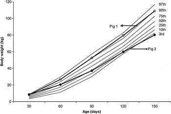
Over the last five decades, pigs have been used extensively in human biomedical research. Using the percentile charts that we have developed in the pig, the identification and the monitoring growth of individuals at increased risk of disease in later life will allow intervention strategies to be explored in more detail. An example of how the weight percentile charts can be used is given in Figure 1. The two animals were reared under normal commercial conditions. An interpretation of the chart shows that at 30 days of age, both pigs weighed ~8 kg and were around the 90th centile. Whilst one pig continued to follow the 90th centile and achieved a weight of 108 kg at 150 days of age, thus demonstrating an ideal pattern of growth, the other pig had fallen through two centiles to the 50th centile by 60 days of age. This pig continued to exhibit poor growth and consequently by day 120 it was on the 10th centile, and by 150 days it was below the 3rd centile, weighing just 80 kg. As this pig failed to maintain its original growth trajectory by dropping through three centiles, it would be considered to be at risk of adulthood disease (Poore et al., Reference Poore, Forhead, Gardner, Giussani and Fowden2002; Poore and Fowden, Reference Poore and Fowden2002, Reference Poore and Fowden2003 and Reference Poore and Fowden2004).
Tracking the growth of two individual pigs from 30 to 150 days of age using the percentile curves for body weight.

Limitations of the LMS model
A variety of methods are available for developing smoothed curves of growth, and produce fairly similar results; however, at present there appears to be no single method that is best in all situations and for all purposes (Flegal, Reference Flegal1999). It should be noted from the outset that any estimates of overweight and underweight may be sensitive to the methods chosen, and so data should be interpreted with care. The LMS method was used in the current study, and it models the whole distribution of the data set and smoothes out any skewness, allowing any desired percentile or Z score to be calculated from the smoothed L, M and S parameters. One of the main benefits of using the growth curves derived from the LMS parameters is that population sampling and measurement errors have less effect on the generated percentiles (Healy, Reference Healy1992). As discussed by Cole and Green (Reference Cole and Green1992), the fitting of smooth centiles curves is subjective as the difficulty lies in deciding whether a bump or dip observed on a centiles curve at a certain age is a real feature of the data, or whether an error has occurred in the measurement itself. One example of this would be the dip in the porcine curve in the immediate post-weaning period, which we know to be a true occurrence rather than an artefact. However, a limitation of the current data set is that we were only able to take monthly measurements post-weaning to avoid causing repeated stress to the animals, which would have resulted in impaired carcass quality. Consequently, our porcine growth charts may be misleading in the short period after weaning because they make no allowance for the initial weight loss observed after weaning nor do they take into account the compensatory growth that is usually seen after the dip in post-weaning weight. In addition, as mentioned above, the changes around puberty would have also caused alterations in growth patterns, and so these curves may not give a true representation of growth patterns around this time frame.
As discussed by Flegal (Reference Flegal1999), an accurate estimation of percentiles from the LMS method relies on the assumption that after transformation and smoothing, the variables (e.g. BW) are normally distributed. These authors examined the validity of this assumption by comparing the distribution of Z scores calculated using smoothed values of L, M and S with a normal distribution curve. They showed that there was a deviation of almost half a s.d. at the upper end of the distribution for one age group, as well as a systematic departure from normality for BW and BMI, highlighting the need for some further transformation. Consequently, it seems feasible to suggest that further transformations may be required to give a more accurate account of pig growth.
Another perceived problem with the LMS method is that the outer tails of the distribution can be influenced by outliers in the data set. In this instance, a restricted application of the LMS method could be used to limit the Box–Cox normal distribution to the interval corresponding to Z scores where empirical data were available. This methodology would prevent assumptions being made about the distribution of data beyond the limits of the observed values (WHO Multicentre Growth Reference Study Group, 2006).
Apart from using these percentile curves, when individuals are weighed and measured at regular intervals, a Z score can be calculated for each measurement allowing for an accurate method of determining if the subject is failing to thrive or exhibiting accelerated growth, thus allowing the opportunity for intervention. Z scores are superior to percentiles, particularly for infants whose size is outside of the normal range of a growth chart, that is, beyond the 3rd and 97th percentiles. Z scores refer to the number of s.d. greater (positive value) or smaller (negative value) than the median (Fenton and Sauve, Reference Fenton and Sauve2007). The changes in Z scores between 30 and 150 days of age were calculated for BW for the two pigs shown in Figure 1. As pig 2 showed a decrease in Z scores for weight by more than 0.67 s.d. scores, this indicates catch-down growth, and thus confirms that the pig is failing to thrive.
In conclusion, as in humans, percentile curves are a useful tool for monitoring the growth of an individual pig. Ultimately, the construction of percentile charts for pigs, similar to those in the present study, will allow a more detailed and precise tracking of growth and development of individual pigs under experimental conditions. Additional data are required to improve the growth curves over the post-weaning period as the time points used were broad and so may miss important features of pig growth and development. There are limitations to the LMS method for smoothing the centile curves and hence further exploration of alternative methods for the construction of smoothed curves is warranted.