2. General perspective on the bifurcation due to the domain size: the role of boundary conditions, shape and dimension

Let us begin with a general question regarding pattern formation: is there a critical domain size below which spatial self-organisation cannot occur? In other words, is there always a bifurcation point if the domain size is considered as a bifurcation parameter? In one dimension, the situation is straightforward and has already been addressed in a general context [Reference Klika, Kozák and Gaffney25]. However, in higher dimensions, the answer is not so clear cut and depends on the dimension, geometry, boundary conditions and what we mean by ‘size’. We first consider an infinite domain and then incorporate boundary conditions through a class of Robin boundary conditions, of which the usual Dirichlet and Neumann conditions are special cases.

Consider two morphogens, $\phi$ and $\psi$ , that diffuse and interact in an infinite $n$ -dimensional space. The dynamics of $\phi$ and $\psi$ are defined by a pair of coupled reaction-diffusion equations,

(1) \begin{align} & \frac {\partial \phi }{\partial t}= \nabla ^2\phi +f(\phi ,\psi ),\\[-10pt]\nonumber \end{align}

(2) \begin{align} & \frac {\partial \psi }{\partial t}=D\nabla ^2\psi +g(\phi ,\psi ), \end{align}

where $\nabla ^2$ is the $n$ -dimensional Laplacian. We implicitly assume that the space has been rescaled so that the diffusion rate of $\phi$ is one. This assumption is not essential and the following results still hold without it, but it allows us to reduce the number of parameters. On the infinite domain, we do not need to specify boundary conditions beyond requiring that the solutions remain bounded everywhere.

Since we seek Turing instabilities, we assume that there is a stable homogeneous stationary solution (HSS), which can be driven unstable in the presence of diffusion [Reference Murray44]. The standard Turing analysis proceeds by linearising around this steady state and using spatial trigonometric perturbations that satisfy the boundary conditions [Reference Maini, Woolley, Bianchi, Hillen, Lewis and Yi36]. This leads to the conclusion that only a bounded interval of wave modes can destabilise.

It should be noted that Turing’s stability condition for a HSS in the absence of diffusion is equivalent to the requirement of a critical domain size below which no instability occurs, but this equivalence holds only under Neumann boundary conditions [Reference Klika, Kozák and Gaffney25]. For Dirichlet and Robin boundary conditions, the stability of the HSS must be imposed as an additional condition, since the zero eigenvalue is fixed, does not vary with the domain size and is not part of the spectrum.

As we are first considering the case of no boundary conditions, we perturb the steady state using a general complex Fourier mode of the form

(3) \begin{equation} \exp (\lambda t + i\mu \boldsymbol{x}), \end{equation}

where $i$ is the imaginary unit. This leads to a continuous spectrum of wave modes $\mu$ that satisfies the dispersion relation [Reference Maini, Woolley, Bianchi, Hillen, Lewis and Yi36]

(4) \begin{equation} 0=\det \left (\lambda \boldsymbol{I}+\mu ^2 \boldsymbol{D}-\boldsymbol{J}\right )\!, \end{equation}

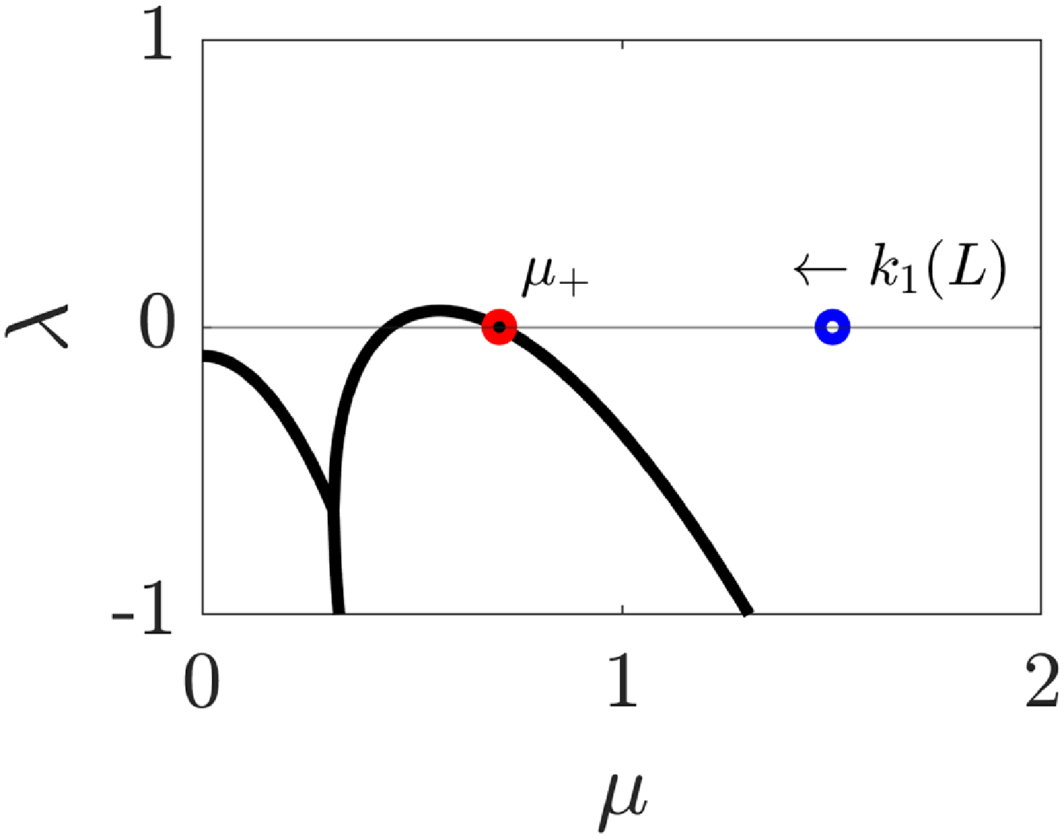
where $\boldsymbol{J}$ is the Jacobian matrix of first-order derivatives of $f$ and $g$ , evaluated at the steady state and $\boldsymbol{D}$ is the diffusion matrix with $1$ and $D$ on the diagonal. A generic form of this dispersion curve is shown in Figure 1, and a full derivation can be found in Section 6.

Figure 1.

The dispersion curve of reaction-diffusion system equations (1) and (2) with Schnakenberg kinetics (18) and (19) and $D=10$ in one spatial dimension. The first non-trivial eigenvalue $k_1(L)$ of the transport operator for the finite one-dimensional domain of length $L$ is highlighted as a blue circle and is calculated explicitly for $L=1$ , resulting in no pattern formation despite the reaction-diffusion parameter values being well within Turing space. The red circle represents $\mu _+=1/\sqrt {2}\approx 0.7071$ , which is the larger solution of equation (4), which assumes an infinite spatial domain. As domain size is increased, $k_1(L)$ decreases as $k_1(L)\propto L^{-2}$ and hence there is a critical domain size for which $k_1(L)=\mu _+$ , the spatial patterning bifurcation point when the domain size, $L$ , is treated as a bifurcation parameter.

From this perspective, the dispersion relation (ignoring transient effects due to nonnormality [Reference Klika24]) links the temporal evolution, through the growth rate $\lambda$ , with the chosen spatial wave mode, treated as a positive parameter $\mu$ . In particular, the dispersion curve, $\Re (\lambda (\mu ))$ , is independent of the spatial dimension considered and boundary information. Critically, only values of $\mu \in [\mu _-,\mu _+]$ for which $\Re (\lambda (\mu ))\gt 0$ correspond to unstable wave modes (see Figure 1).

Suppose we now consider a finite domain $\Omega$ with boundary $\partial \Omega$ on which we define Robin boundary conditions. The spectrum becomes (for a sufficiently regular domain) a discrete set of wave modes $k_i$ , which satisfy

(5) \begin{equation} -\nabla ^2 \gamma = k_i^2 \gamma \mbox{ in }\Omega , \qquad \alpha \gamma + \frac {\partial \gamma }{\partial n} = 0 \mbox{ at } \partial \Omega . \end{equation}

Let us first focus on a one-dimensional problem, hence without loss of generality $\Omega =(0,L)$ . The spectrum for Robin boundary conditions can be calculated directly, and in one dimension, one can observe that the eigenvalues of the Laplacian decrease monotonically with the domain size for both boundary conditions. In particular, as the domain size increases, the lowest eigenvalue decreases as $k_1(L)\propto L^{-2}$ [Reference Klika, Kozák and Gaffney25], and, thus, there is a critical domain size at which the lowest eigenvalue reaches the critical value $k_1=\mu _+$ . For larger values of $L$ , a spatial pattern in $(\phi ,\psi )$ can form [Reference Woolley68]. Therefore, if we consider Turing’s diffusion-driven instability, the existence of a critical size $L_{c}$ follows.

This viewpoint allows the infinite space dispersion curve (which depends only on the reaction kinetics and diffusion coefficients) to be fixed. Information about the pure point spectrum of the Laplacian (which varies due to having a finite domain and boundary conditions) and the transport operator can then be compared with the infinite space dispersion curve. In higher dimensions, the situation is more complex.

2.1. Dirichlet Laplacian

For Dirichlet boundary conditions, the existence of a critical domain size in arbitrary dimension can still be established using geometric spectral theory. For the Dirichlet Laplacian, the spectrum is monotone with respect to domain inclusion [Reference Davies13]. In particular, if $\Omega _1$ , $\Omega _2\subset \mathbb{R}^d$ are arbitrary open sets then

\begin{equation*} \Omega _1 \subset \Omega _2 \quad \Rightarrow \quad k_n^D(\Omega _1)\geq k_n^D(\Omega _2) \quad \forall n\in \mathbb{N}, \end{equation*}

where $k_n^D$ denotes the $n$ th discrete eigenvalue of the Dirichlet Laplacian.

In addition, the isoperimetric (isochoric) Rayleigh–Faber–Krahn inequality [Reference Benguria, Linde and Loewe8] states that for a given ball domain, $B$ , with volume $|B|$

(6) \begin{equation} \min _{|\Omega |=|B|} k_1^D(\Omega ) = k_1^D(B). \end{equation}

Combining these observations with the dispersion relation in Figure 1, we conclude that for Dirichlet boundary conditions, there is a critical domain size (volume) below which no pattern can occur due to Turing’s instability. Moreover, among all domains of a given volume, the ball is the first to exhibit a pattern.

2.2. Neumann Laplacian

The situation is very different for Neumann boundary conditions. First, consider a rectangle $[0,a]\times [0,b]$ with corresponding spectrum $\left ( k_{n,m}^N\right )^2=\left ({n\pi }/{a}\right )^2+\left ({m\pi }/{b}\right )^2$ for $m,\,n\in \mathbb{N}$ [Reference Murray43]. For a given area, the first non-zero eigenvalue has no positive lower bound, since $k_1^N=\min \{k_{10}^N,k_{01}^N\}$ can be made arbitrarily small. Even among convex domains, we therefore cannot expect a critical domain size (volume) to exist.

Monotonicity also fails even among convex domains. This can be seen by comparing the spectra of an inscribed thin rectangle and a larger rectangle circumscribed around it, oriented along their diagonals. As an illustrative example, consider the case in Figure 1, where the critical square side length for patterns to occur is $L_{\text{square}}=\sqrt {2}\pi$ . Patterns can occur on rectangles with one side length greater than $L_{\text{square}}$ , but not on rectangles where both side lengths are less than $L_{\text{square}}$ . In Figure 2, we consider two squares of side length $L_{\text{square}}+0.1$ (blue square) and $L_{\text{square}}-0.1$ (red square). The red square lies entirely within the blue square, and we expect Turing patterns to appear on the blue square, but not on the red square, which is confirmed by the simulation results in the lower panel of Figure 2. However, inside the red square, we can fit a rotated rectangle of side length $L_{\text{square}}+0.1$ (black rectangle), and we observe that the black rectangle can also support patterns even though it is smaller than the red square, which cannot pattern.

Figure 2.

Illustration of the non-monotonicity of Turing patterns on two-dimensional domains with Neumann boundary conditions. In the top panel, we compare the domain geometries and see that the black rectangle is a subdomain of the red square, which is a subdomain of the blue square. In the bottom panel, we visualise $\phi$ as simulated from equations (1) and (2) on these domains with Schnakenberg kinetics (18) and (19) and $D=10$ , patterns appear on the blue square and black rectangle only.

An isoperimetric (isochoric) inequality is available in this setting, the Szegö–Weinberger inequality [Reference Benguria, Linde and Loewe8],

(7) \begin{equation} \max _{|\Omega |=|B|} k_1^N(\Omega ) = k_1^N(B), \end{equation}

which provides an upper bound for the first non-zero Neumann eigenvalue (in contrast with the lack of a positive lower bound, noted earlier). Thus, for Neumann boundary conditions, the ball is the last geometry to support a pattern for a given volume.

Therefore, neither of the two key properties used for Dirichlet conditions, namely monotonicity and a positive lower bound on the first eigenvalue in terms of volume, is available for Neumann boundary conditions. Moreover, the spectrum of the Neumann Laplacian can be highly sensitive to changes in geometry [Reference Arcuri and Murray5, Reference Benguria, Linde and Loewe8, Reference Davies13, Reference Hale18]. It is possible to alter the spectrum by an arbitrary amount through changes in an arbitrarily small neighbourhood of a single point. If the boundary is not sufficiently smooth, the Laplacian may even have an essential spectrum. A sufficient condition for the spectrum of the Neumann Laplacian to be purely discrete is that the domain is bounded with a Lipschitz boundary [Reference Davies13]. Under suitable regularity conditions, two domains that are close in shape will have spectra that are close in an appropriate sense [Reference Burenkov and Davies10]. Nevertheless, this result is given in a precise mathematical sense (as an estimate with an undetermined constant) and hence cannot be used for practical applications to estimate how large the difference in spectra is for two given domains.

We can therefore conclude that a critical domain size (measured using its volume) does not exist in general for Neumann boundary conditions, even if the domains are sufficiently regular. There are, however, two notable classes of domains for which a bifurcation point appears as the size of the domain changes. The first consists of isotropically scaled domains of the form $\Omega =l \Omega _0$ for a fixed $\Omega _0$ , where the spectrum of the Neumann Laplacian scales as $k_n^N(l \Omega _0)=k_n^N(\Omega _0)/{l^2}$ . The existence of a critical domain size in one-dimensional domains is a special case of this, since any change in the domain is a simple scaling. The second class is that of convex domains, which have a critical size measured by the diameter rather than by volume or surface area.

For convex domains, Payne and Weinberger [Reference Payne and Weinberger49] showed that the infimum of the spectrum for domains with a given diameter is strictly positive. In particular, for convex domains $\Omega$ with diameter $d=\sup _{\boldsymbol{x},\boldsymbol{y}\in \Omega }\{|\boldsymbol{x}-\boldsymbol{y}|\}$ , the following inequality holds:

(8) \begin{equation} k_1^N(\Omega ) \geq \frac {\pi ^2}{d^2}. \end{equation}

This gives a lower bound on the first non-trivial eigenvalue in terms of a one-dimensional measure of the size of the convex domain, namely the length of the longest line segment that can be contained in $\Omega$ . A similar inequality holds for symmetric domains, for which the intersection of the domain with any line in a coordinate direction is simply connected [Reference Payne and Weinberger48]. For non-convex domains, this property does not hold in general.

2.3. Robin Laplacian

As we have seen, one needs a combination of two properties of the spectrum to have the existence of the critical domain size: (i) monotonicity and (ii) a lower bound for the spectrum (via isochoric or isoperimetric inequality). For Dirichlet Laplacian both were available, while for Neumann we lack both (there is no monotonicity in general and neither is there a lower bound on the spectrum).

For a general Robin boundary condition with $\alpha \gt 0$ , the spectral lower bound is available (for regular enough domains to have a pure point spectrum) due to the following Bossel–Daners isochoric inequality [Reference Benguria, Linde and Loewe8]:

(9) \begin{equation} \min _{|\Omega |=|B|} k_1^R(\Omega ) = k_1^R(B), \end{equation}

where $B$ is a ball, noting that for $\alpha \lt 0$ a similar statement is still an open problem in spectral theory [Reference Krejčiřík and Lotoreichik31]. However, the second necessary property, the monotonicity of spectrum with respect to domain size, does not hold for the Robin Laplacian and hence we cannot combine them to show the existence of a critical domain size.

3. Parallelogram geometry

Due to the issues raised in Section 2.2, we focus on the convex domain of a parallelogram. Explicitly, a parallelogram is a quadrilateral where opposite sides have equal length, but, generally, the length of each pair of sides will be different. As such, a parallelogram can be parametrised by its two side lengths, $L_1$ and $L_2$ , and its interior angle, $\theta$ . 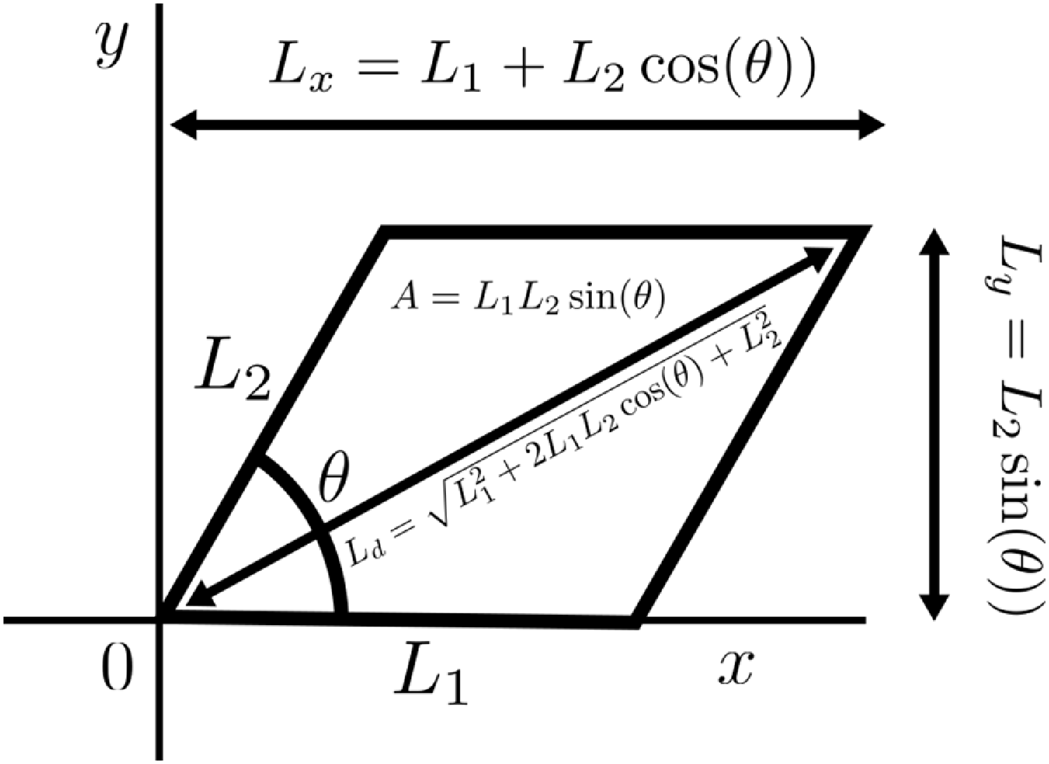From this parametrisation, we can define the height of the parallelogram, $L_y$ ; its total width, $L_x$ ; its longest diagonal, $L_d$ ; and its area, $A$ (see Figure 3).

Figure 3.

Defining the geometry of the parallelogram using: its side lengths, $(L_1,L_2)$ , and interior angle $\theta$ ; the derived lengths, $(L_x,L_y,L_d)$ ; and its area, $A$ .

Before dealing with Turing bifurcations on parallelograms in their full complexity, we are going to consider two subcases (see Figure 4). First, we are going to consider the case of the rhombus, where the lengths of the parallelogram’s sides are all equal, $L_1=L_2=L$ . As mentioned in Section 1, we will seek to link how the Turing patterning bifurcation side length, $L_{rhombus}$ , depends on $\theta$ .

Second, we are going to consider the case of creating a parallelogram from shearing a square (denoted the sheared parallelogram case). Here, we start with a square of side length $L_1(\pi /2)=L_2(\pi /2)=L$ . This square is then sheared such that the base length, $L_1$ , and height, $L_y$ , are fixed, meaning that $L_2=L/\sin (\theta )$ . We look to extract the relationship between the Turing patterning bifurcation side length and the shearing angle, $L_{sheared}(\theta )$ . Since all sheared parallelograms have the same area as the initial square, $A=L^2$ , this will inform us of how sheared an area has to be before a Turing pattern can be formed.

Finally, we consider the case of a completely arbitrary parallelogram, where the parameters $(L_1,L_2,\theta )$ are not geometrically coupled. Rather, we seek to extract the relationship between critical lengths $(L_{1c}(\theta )$ and $L_{2c}(\theta ))$ that specifies how big the sides of a parallelogram have to be to induce a Turing instability.

In all cases, we will be specifically interested in the limit of $\theta \rightarrow 0$ since in this limit the parallelograms will be tending to one-dimensional domains of length $L_x=L_1+L_2$ , where $\lim _{\theta \rightarrow 0} L_d=L_x$ . Thus, we will be able to see how the Turing patterning bifurcation domain size compares across the one-dimensional parallelogram limits, as well as with a simple one-dimensional Turing analysis, where the critical length, $L_{square}$ , can be defined algebraically (see Section 6).

4. Equation mapping

To analyse and simulate Turing bifurcations on parallelograms, we need to define the Laplacian on the domain. Either we can work directly on the parallelogram, using the standard Euclidean Laplacian,

(10) \begin{equation} \nabla ^2_{(x,y)}=\frac {\partial ^2 }{\partial {x}^2}+\frac {\partial ^2 }{\partial {y}^2}, \end{equation}

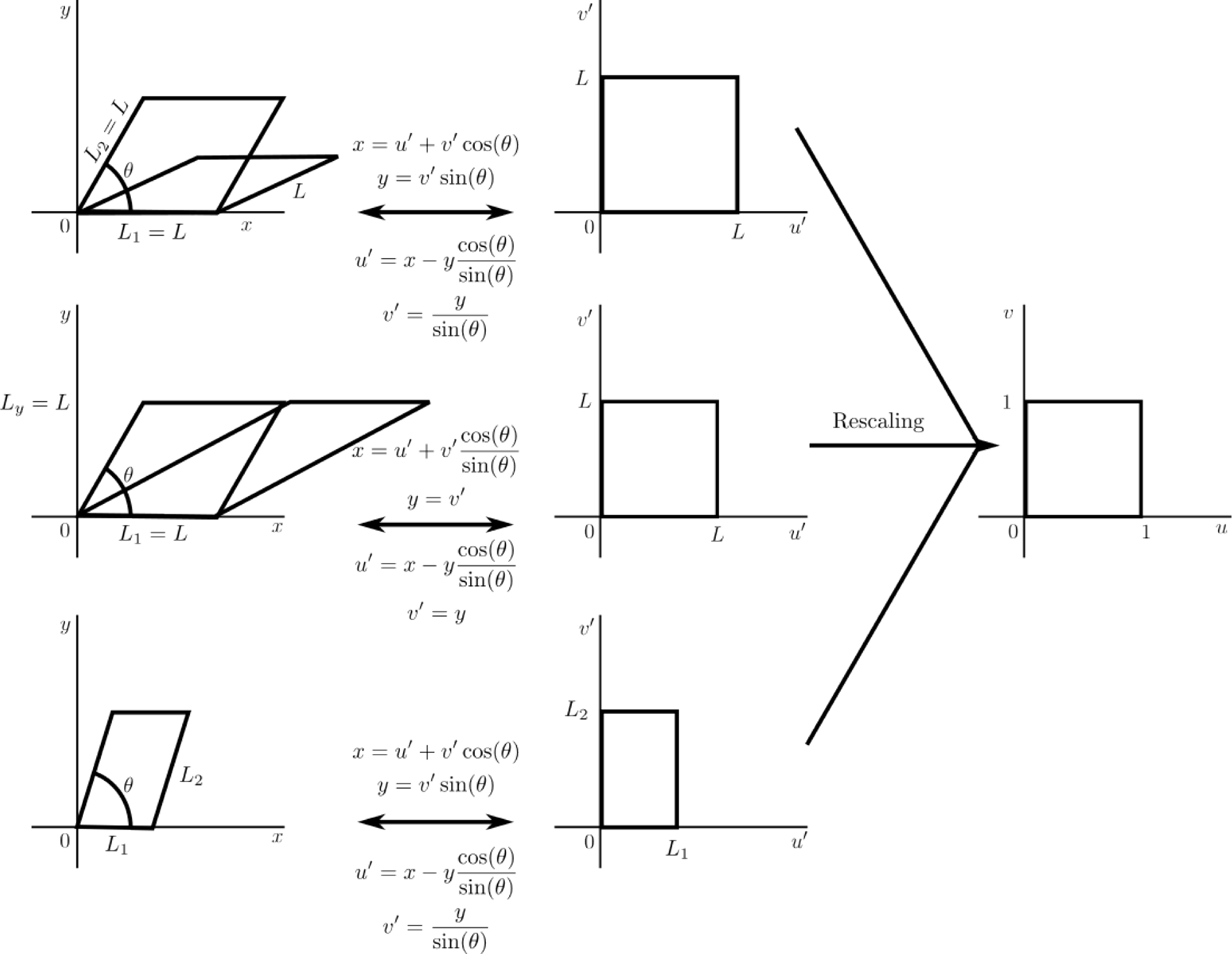
or we can map the shape to a regular square [Reference Kuttler and Sigillito32, Reference Lewin and Stjernstoft34] (see Figure 4).

In the case of the rhombus, all side lengths are the same constant, which is independent of $\theta$ . Thus, finding the bifurcation length becomes a case of scaling the whole space, which does not change the parallelogram’s aspect ratio, $L_2/L_1$ . Thus, we can work with both the original and mapped domains, providing evidence that mapping does not influence the Turing bifurcation structure.

In the sheared and general cases, however, the side lengths $L_1$ and $L_2$ depend on $\theta$ . Thus, as we iterate over $\theta$ , the aspect ratio of the parallelogram will change meaning that it is easier to simulate and track bifurcations on the mapped square space, rather than continuously remeshing the changing geometry.

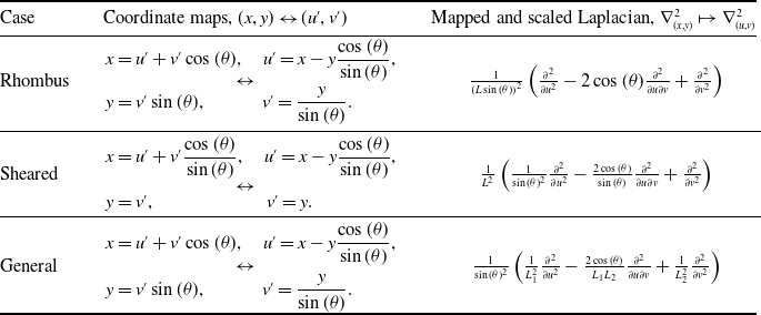
Table 1 provides the coordinate maps and scaled and mapped Laplacians in all three parallelogram cases. Although the rhombus and sheared parallelogram cases are subcases of the full general case, their geometric restrictions produce simpler Laplacians, which are useful to highlight, due to a previously recorded error [Reference Lewin and Stjernstoft34].

Table 1.

Coordinate mappings and Laplacians for the three parallelogram cases. Compare with Figure 4.

Table 1. Long description

Panel A: Rhombus. The coordinate maps are given by x equals u prime plus v prime times the cosine of theta, u prime equals x minus y times the cosine of theta divided by the sine of theta, y equals v prime times the sine of theta, and v prime equals y divided by the sine of theta. The mapped and scaled Laplacian is one divided by the product of L and the sine of theta, times the second derivative of u prime squared plus the second derivative of v prime squared minus two times the cosine of theta times the mixed derivative of u prime and v prime. Panel B: Sheared. The coordinate maps are given by x equals u prime plus v prime times the cosine of theta divided by the sine of theta, u prime equals x minus y times the cosine of theta divided by the sine of theta, y equals v prime, and v prime equals y. The mapped and scaled Laplacian is one divided by L squared, times the second derivative of u prime squared plus the second derivative of v prime squared minus two times the cosine of theta divided by the sine of theta times the mixed derivative of u prime and v prime. Panel C: General. The coordinate maps are given by x equals u prime plus v prime times the cosine of theta, u prime equals x minus y times the cosine of theta divided by the sine of theta, y equals v prime times the sine of theta, and v prime equals y divided by the sine of theta. The mapped and scaled Laplacian is one divided by the product of the sine of theta and L1 squared, times the second derivative of u prime squared plus one divided by the product of the sine of theta and L2 squared, times the second derivative of v prime squared plus two times the cosine of theta divided by the product of L1, L2, and the sine of theta, times the mixed derivative of u prime and v prime.

Figure 4.

Mapping parallelograms to the unit square. Top: rhombus. The lengths of each side are the same. Middle: sheared parallelogram. The parallelogram maintains the same area as it is sheared since its height, $L_y=L$ remains fixed as $\theta$ changes. Bottom: general parallelogram.

5. Eigenvalue bounds

To apply Turing analysis to reaction-diffusion equations on parallelogram spaces, we need to be able to solve

(11) \begin{equation} \nabla ^2 \gamma =-k^2\gamma \end{equation}

with zero-flux boundary conditions on either the original parallelogram or mapped space. Unfortunately, explicit solutions to equation (11) are known in very few cases [Reference McCartin40–Reference McCartin42, Reference Woolley65, Reference Woolley66]. However, much work has been done on bounding the eigenvalues, $k$ , of general shapes [Reference Bandle6, Reference Laugesen and Siudeja33, Reference Szegö58, Reference Weidl, Benguria, Ashbaugh and Laugesen64].

It is known [Reference Laugesen and Siudeja33, Reference Szegö58] that for closed, bounded domains with Lipschitz continuous boundaries equation (11) has an infinite sequence of eigenvalues, $\{k_i\}^\infty _{i=1}$ , such that

(12) \begin{equation} 0=k_0^2(\Omega )\lt k_1^2(\Omega )\lt \dots , \end{equation}

where we know that the lowest eigenvalue is $k_0=0$ since a constant $\gamma$ is a solution to equation (11) with Neumann boundary conditions for any constant value.

Critically, the main result of Léna and Rohleder [Reference Léna and Rohleder35] focuses on bounding $k_1$ for parallelograms using inequalities involving $(L_1,L_2,\theta )$ . If we define

(13) \begin{gather} C_1(L_1,L_2,\theta )=\frac {\pi ^2}{2A^2}\left ( L_1^2+L_2^2-\sqrt {(L_1^2-L_2^2)^2+\frac {256}{\pi ^4}L_1^2L_2^2\cos (\theta )^2}\right )\!, \end{gather}

(14) \begin{gather} C_2(L_1,L_2,\theta )=\frac {6}{A^2}\left ( L_1^2+L_2^2-\sqrt {(L_1^2-L_2^2)^2+4L_1^2L_2^2\cos (\theta )^2}\right )\!, \end{gather}

where $A=L_1L_2\sin (\theta )$ is the area of the parallelogram then [Reference Léna and Rohleder35]

(15) \begin{align} k_1^2\leq \min \left \{ C_1(L_1,L_2,\theta ), C_2(L_1,L_2,\theta ) \right \}\!. \end{align}

In the case of a rhombus, $L_1=L_2=L$ , the result simplifies to

(16) \begin{equation} k_1^2\leq \min \left \{ \frac {\pi ^2}{L^2\sin (\theta )^2}\left (1-\frac {8}{\pi ^2}|\cos (\theta )|\right ),\frac {12}{L^2\sin (\theta )^2}\left (1-|\cos (\theta )|\right ) \right \}\!, \end{equation}

where inequality (16) becomes an equality, $k_1^2=\pi ^2/L^2$ , in the specific case that $\theta =\pi /2$ and the rhombus is a square. In the case of the sheared parallelogram, $(L_1,L_2)=(L,L/\sin (\theta ))$ , the result becomes

(17) \begin{align} k_1^2 & \leq \min \left \{ \frac {\pi ^2}{2L^2\sin (\theta )^2}\left ( 2-\cos (\theta )^2\left ( 1+\sqrt {1+\frac {256}{\pi ^4}\tan (\theta )^2}\right )\right )\!,\right.\nonumber\\[5pt]& \quad \frac {6}{L^2\sin (\theta )^2}\left ( 2-\cos (\theta )^2\left ( 1+\sqrt {1+4\tan (\theta )^2}\right )\right ) \Bigg\}\!. \end{align}

Critically, inequalities (16) and (17) can be rearranged to form inequalities of the form $L\leq L_{C}(k_1,\theta )$ , where $L_C$ will be an upper bound for the Turing patterning bifurcation size. In the general parallelogram case, we need to vary our simulations not just over $\theta$ , but over aspect ratios, $a=L_2/L_1$ , as well. Inequality (15) can then be written in the form $L_1\leq L_{C}(a,k_1,\theta )$ , from which we get an upper bound on the Turing patterning bifurcation size of $L_1$ , and $L_2=aL_1$ .

6. Turing kinetics

When dealing with theory and analysis, we will keep the parameters and kinetics general. However, we will demonstrate the results using a specific form of the Schnakenberg kinetics [Reference Schnakenberg53],

(18) \begin{align} &f(\phi ,\psi )=\frac {1}{10}-\phi +\phi ^2\psi ,\\[-8pt]\nonumber \end{align}

(19) \begin{align} &g(\phi ,\psi )=\frac {9}{10}-\phi ^2\psi , \end{align}

with $D=10$ .

Since we are assuming a Turing instability occurs then, $f(\phi ,\psi )$ and $g(\phi ,\psi )$ , permit a stable steady state, $(\phi _s,\psi _s)$ , in the absence of diffusion that can be driven unstable when diffusion is included. Deriving stability conditions for steady states in the diffusion-free case is a fairly simple linearisation argument about the steady state, where the perturbation only depends on time [Reference Murray45]; thus, this stability argument does not include any information regarding the spatial aspects of the problem.

As mentioned in Section 2, we first consider the infinite space case by extending the perturbation to include a spatial component of the form (3), which provides a range of wave modes, $[\mu _-,\mu _+]$ , that will be unstable [Reference Woolley66, Reference Woolley69],

(20) \begin{equation} \mu ^2_\pm =\frac {g_\psi + Df_\phi \pm \sqrt {(g_\psi + Df_\phi )^2 - 4D(f_\phi g_\psi - g_\phi f_\psi )}}{2D}. \end{equation}

Substituting equations (18) and (19) into equations (20) and (24), we find that $\mu _+=1/\sqrt {2}$ in the specific case of the Schnakenberg kinetics.

Having derived the infinite space solution, we now consider reaction-diffusion system (1) and (2) occurring on the parallelogram domain, $\Omega (L_1,L_2,\theta )$ with zero-flux boundary conditions,

(21) \begin{equation} {\left .\kern -1pt {\frac {\partial \phi }{\partial \boldsymbol{n}}} \vphantom {\big |} \right |_{\partial \Omega } }=0= {\left .\kern -1pt {\frac {\partial \psi }{\partial \boldsymbol{n}}} \vphantom {\big |} \right |_{\partial \Omega }}, \end{equation}

where $\partial /\partial \boldsymbol{n}$ is the derivative along the outward pointing normal, $\boldsymbol{n}$ , on the boundary. Although non-trivial to explicitly define for the general parallelogram case in the $(x,y)$ shape space, the normal derivatives simplify to the horizontal and vertical derivatives in the mapped $(u,v)$ coordinates.

We consider zero-flux boundary conditions due to their simplicity and generality in that they are often used in biological scenarios as a means of modelling boundaries that do not influence the internal kinetics [Reference Murray44]. This work could be repeated in the case of Dirichlet, or mixed Dirichlet-Neumann, boundary conditions as similar results bounding the first non-zero eigenvalue of the Laplacian exist in these cases [Reference Aldeghi and Rohleder1, Reference Antunes and Henrot2, Reference Henrot20].

In the simple case of the one-dimensional line, or two-dimensional square, we can analytically solve equation (11) in terms of trigonometric functions, providing a dispersion relation between the domain’s size, $L$ , and the spatial frequencies, $k_n=n\pi /L$ (in 1D) and $k_{n,m}=\sqrt {(n\pi /L)^2+(m\pi /L)^2}$ (in 2D), which will be unstable [Reference Woolley, Krause and Gaffney74]. In the case of the square, the derivation of the smallest bifurcation length decouples into the perpendicular Cartesian directions, meaning that it is effectively a one-dimensional derivation [Reference Woolley67]. Thus, the bifurcation length of the line will be the same as the critical side length of the square. Since the eigenvalue and the domain size are related through $L=\pi /k$ , the critical length of the line, or square ( $n=1$ , $m=0$ case), is $L_{square}=\sqrt {2}\pi \approx 4.44$ .

In the case of the rhombus and the sheared parallelogram, we have removed one of the degrees of freedom from the full general parallelogram case. Thus, we only need to consider one length scale, $L$ , and its relation to the internal angle. Since as $L$ grows $k_1$ decreases, then the first bifurcation will occur when $k_1=\mu _+$ (see Figure 1). Thus, substituting $k_1=\mu _+$ in the bounds derived in Section 5 allows us to evaluate the upper bounds on the critical size of a parallelogram on which a Turing pattern will begin to appear.

7. Rhombus

To numerically derive the relationship between the parallelogram’s side lengths and the internal angle that will produce a Turing instability for each $\theta$ , we will use pseudo-arc length continuation with a predictor-corrector method as built into the numerical bifurcation package, pde2path, version 3.0 [Reference Dohnal, Rademacher, Uecker, Wetzel, Ecker, Steindl and Jakubek14, Reference Engelnkemper, Gurevich, Uecker, Wetzel and Thiele15, Reference Uecker61, Reference Uecker, Wetzel and Rademacher62]. The numerically extracted bifurcation lengths are then tested with COMSOL Multiphysics 6.1 [11], as we simulate the full non-linear spatio-temporal equations with parameters that correspond to before and after the critical bifurcation values. All of the following simulation scripts and files can be found at https://github.com/ThomasEWoolley/Turing_parallelogram.

In the case of the rhombus, we want to extract the bifurcation relationship between the side length, $L$ , and the internal angle, $\theta$ , and we define this relationship to be $L_{rhombus}(\theta )$ . Although we vary $\theta$ between 0 and $\pi /2$ , each simulation is run with fixed $\theta$ . The critical size is then extracted using pde2path, which finds the first point at which an instability occurs as $L$ is increased. Since varying $L$ rescales space, the parallelograms will still be congruent and similar in the geometric sense. Thus, we can simulate on the original parallelogram space using the rescaled Laplacian $(x,y)\mapsto (Lx',Ly')$ ,

(22) \begin{equation} \nabla ^2_{(x,y)}=\frac {1}{L^2}\nabla ^2_{(x',y')}, \end{equation}

as well as the mapped square space (see Table 1)

(23) \begin{equation} \nabla ^2_{(x,y)}=\frac {1}{L^2\sin (\theta )^2}\left ( \frac {\partial ^2 }{\partial {u}^2}{} -2\cos (\theta )\frac {\partial ^2}{\partial u \partial v} +\frac {\partial ^2 }{\partial {v}^2}{}\right )\!. \end{equation}

The benefit of scaling the Laplacian as in equation (22) is that the size becomes a parameter within the simulation, and the geometry is fixed.

As mentioned in Section 5, we can rearrange inequality (16) to generate

(24) \begin{equation} L_{rhombus}(\theta )\leq \min \left \{ L_{C1}(\mu _+,\theta ),L_{C2}(\mu _+,\theta ) \right \}=L_{C}(\mu _+,\theta ), \end{equation}

where

(25) \begin{align} &L_{C1}(\mu _+,\theta )=\sqrt {\frac {\pi ^2}{\mu _+^2\sin (\theta )^2}\left (1-\frac {8}{\pi ^2}|\cos (\theta )|\right )},\\[-7pt]\nonumber \end{align}

(26) \begin{align} &L_{C2}(\mu _+,\theta )=\sqrt {\frac {12}{\mu _+^2\sin (\theta )^2}\left (1-|\cos (\theta )|\right )}. \end{align}

Note that $L_{C1}(\mu _+,\theta )=L_{C2}(\mu _+,\theta )$ when

\begin{equation*} \theta =\theta _T=\arctan \left (\frac {\sqrt {(\pi +4)(4-\pi )(\pi ^2-8)}}{12-\pi ^2}\right )\approx 1.01 \end{equation*}

whence we can define the piecewise bound

\begin{equation*} L_{C}(\mu _+,\theta )=\left \{ \begin{array}{ll} L_{C1}(\mu _+,\theta ), & \theta \geq \theta _T, \\[3pt] L_{C2}(\mu _+,\theta ), & \theta \lt \theta _T, \end{array} \right . \end{equation*}

and we will compare this bound to numerically derived data.

Figure 5 illustrates $L_{rhombus}(\theta )$ as numerically derived from the unmapped and mapped spaces, as well as the bounds $L_{C1}$ and $L_{C2}$ . First, we note the excellent comparison of the numerically extracted critical lengths in both the mapped and unmapped simulations (see Figure 5a). Equally, we observe that these numerically extracted values of $L_{rhombus}(\theta )$ are tight bounds because patterns only appear when $L\gt L_{rhombus}$ for a given fixed $\theta$ (see Figure 5e).

We note that $\min _\theta L_{rhombus}(\theta )=L_{rhombus}(0)\approx 3.41\leq L_{rhombus}(\theta )\leq L_{square}$ ; thus, the bifurcating rhombus will always have a smaller side length than the square. However, it makes more sense to compare $L_{square}$ with $L_x$ (see Figure 5b), which is the horizontal width of the rhombus (see Figure 3). Critically, we may expect $L_x(\theta )=L_{square}$ when $\theta =\pi /2$ and 0 because in both cases we reduce to a separable, or literal, one-dimensional analysis, respectively. We observe that when $\theta =\pi /2$ , the rhombus becomes a square and the bifurcation results and theory exactly match the square case, namely, $L_{rhombus}(\pi /2)=L_{square}=\sqrt {2}\pi$ [Reference Woolley66]. However, as $\theta \rightarrow 0$ , we see that $L_x$ converges to a higher value than expected and is bounded by $3L_{square}/2\approx 6.66\lt 2L_{rhombus}(0) \lt 2L_{C2}(\mu _+,0)=2\sqrt {6}/\mu _+=2\sqrt {12}\approx 6.93$ (see Figure 5b). Thus, we observe that the one-dimensional limit of the bifurcation width of the rhombus is larger than the one-dimensional line.

Figure 5.

(a) Numerically derived critical lengths, $L_{rhombus}$ , using mapped and unmapped geometries, compared against the bounds $L_{C1}$ and $L_{C2}$ from equations (25) and (26), respectively (see legend). The upper and lower dashed lines represent $L_{square}=\sqrt {2}\pi$ and $L_{square}/2$ , respectively. (b) Critical total horizontal widths, $L_x=L(1+\cos (\theta ))$ , where $L$ is $L_{rhombus}$ (as derived from the mapped and unmapped geometries), $L_{C1}$ and $L_{C2}$ . The upper and lower dashed lines represent $2L_{square}$ and $L_{square}$ , respectively. (c) Critical diagonal lengths, $L_d=\sqrt {2}L\sqrt {1+\cos (\theta )}$ , where $L$ is $L_{rhombus}$ (as derived from the mapped and unmapped geometries), $L_{C1}$ and $L_{C2}$ . The dashed line represents $\sqrt {2}L_{square}$ . (d) Critical areas, $A=L^2\sin (\theta )$ , where $L$ is $L_{rhombus}$ (as derived from the mapped and unmapped geometries), $L_{C1}$ and $L_{C2}$ . The line colours across (a)-(d) are consistent and defined in the legend of (a). (e) Simulating Turing patterns on the rhombuses of angle $\theta =\pi /2$ (trivial square) and 0.1 before the critical bifurcation length (left) and after (right). $L=4.4$ and $4.5$ for the square in the left and right graphs, respectively. $L=3.3$ and $3.5$ for the $\theta =0.1$ rhombus in the left and right graphs, respectively.

Figure 5. Long description

Panel A: A line graph compares numerically derived critical lengths using mapped and unmapped geometries against bounds from equations. The x-axis represents theta, and the y-axis represents L. The upper and lower dashed lines represent specific bounds. Panel B: A line graph shows critical total horizontal widths against theta. The upper and lower dashed lines represent specific bounds. Panel C: A line graph displays critical diagonal lengths against theta. The dashed line represents a specific bound. Panel D: A line graph illustrates critical areas against theta. Panel E: Two color gradient plots simulate Turing patterns on rhombuses of different angles before and after the critical bifurcation length.

As an alternative metric, in Figure 5c, we consider the longest diagonal of the rhombus, $L_d$ . We observe that $L_d$ is always between the dashed line, which represents the diagonal of the square $\sqrt {2}L_{square}$ (and they are equal when $\theta =\pi /2$ ) and the value of $L_d$ that uses the $L_{C2}$ bound, which we note is constant, $L_d(L_{C2})=4\sqrt {3}\approx 6.93$ for all $\theta$ . Comparing Figure 5b and c shows that $L_x$ and $L_d$ have similar curve shapes and indeed $\lim _{\theta \rightarrow 0} L_d(\theta )=\lim _{\theta \rightarrow 0} L_x(\theta )$ because the diagonal and total horizontal widths collapse onto one another in the pseudo-one-dimensional case.

Although we see that the limits $L_{C1}$ and $L_{C2}$ act as good approximations to $L_{rhombus}$ , we note that the actual form of $L_{rhombus}(\theta )$ is not known. However, Figure 5d suggests that the area of the rhombus decreases approximately linearly as $\theta \rightarrow 0$ . Since the area must go through $A(0)=0$ and $A(\pi /2)=L_{square}^2=2\pi ^2$ , the straight line connecting these two points is $f(\theta )=4\pi \theta$ , further the area is just below this line for all $\theta$ , so $A\lesssim 4\pi \theta$ , or $L_{rhombus}(\theta )\lt \sqrt {4\pi \theta /\sin (\theta )}=L_{C3}(\theta )$ , which is a new uniform smooth bound, which can be compared against piecewise $L_C$ .

We find the maximum error between $L_{rhombus}$ and $L_{C3}$ is smaller than the maximum error between $L_{rhombus}$ and $L_{C}$ , which occurs at $\theta _T$ ,

\begin{equation*} \max _\theta \left ( L_{C3}(\theta )-L_{rhombus}(\theta )\right )\approx 0.15\lt 0.20\approx \max _\theta \left ( L_{C}(\theta )-L_{rhombus}(\theta )\right )\!. \end{equation*}

However, the average error across the $\theta$ interval is still smaller for the piecewise form,

\begin{equation*} \frac {2}{\pi }\int ^{\pi /2}_0 L_{C}(\theta )-L_{rhombus}(\theta )\text{ d} \theta \approx 0.09\lt 0.11 \approx \frac {2}{\pi }\int ^{\pi /2}_0 L_{C3}(\theta )-L_{rhombus}(\theta )\text{ d} \theta . \end{equation*}

8. Sheared parallelogram

Following the approach in Section 7, we numerically extract the critical relationship between the length scale, $L$ , and the internal angle, $\theta$ , at which the parallelogram will first bifurcate into patterns (see Figure 6a). Specifically, if we fix $L\lt L_{square}$ and we shear the subsequent square into a parallelogram, then all of the shapes will have the same area $A=L^2$ (see Figure 3); however, as the shape is sheared with decreasing $\theta$ , its horizontal length, $L_x$ (Figure 6b), and longest diagonal, $L_d$ (Figure 6c), become larger; thus, the space will eventually pattern. Indeed, from equation (17), we find that

(27) \begin{equation} L_{sheared}(\theta )\leq \min \{L_{C1}(\mu _+,\theta ),L_{C2}(\mu _+,\theta )\} \end{equation}

where, in this case,

(28) \begin{gather} L_{C1}(\mu _+,\theta ) = \sqrt {\frac {\pi ^2}{2\mu _+^2\sin (\theta )^2}\left ( 2-\cos (\theta )^2\left ( 1+\sqrt {1+\frac {256}{\pi ^4}\tan (\theta )^2}\right )\right )}, \end{gather}

(29) \begin{gather} L_{C2}(\mu _+,\theta ) = \sqrt {\frac {6}{\mu _+^2\sin (\theta )^2}\left ( 2-\cos (\theta )^2\left ( 1+\sqrt {1+4\tan (\theta )^2}\right )\right )} . \end{gather}

Similar to Figure 5, we observe in Figure 6 that $L_{C1}$ and $L_{C2}$ provide excellent bounds separating the $(L,\theta )$ parameter region that will pattern from the region that does not (compare Figures 5a and 6a). However, there are distinct differences between the critical size of the rhombus and the sheared parallelogram. For example, as $\theta \rightarrow 0$ the side length of the rhombus tends to a finite non-zero limit, $L_{rhombus}(0)\approx 3.41$ , whereas the side length of the sheared parallelogram tends to $L_{sheared}(0)=0$ .

Figure 6.

(a) Numerically derived critical lengths, $L_{sheared}(\theta )$ , compared against the bounds $L_{C1}$ and $L_{C2}$ from equations (28) and (29), respectively. The dashed line represent $L_{square}=\sqrt {2}\pi$ . (b) Critical total lengths, $L_x=L(1+\cos (\theta )/\sin (\theta ))$ , where $L$ is $L_{sheared}$ , $L_{C1}$ or $L_{C2}$ . The dashed line represents $L_{square}$ . (c) Critical diagonal lengths, $L_d=L\sqrt {1+(1+1/\tan (\theta ))^2}$ , where $L$ is $L_{sheared}$ , $L_{C1}$ or $L_{C2}$ . The upper and lower dashed lines represent $\sqrt {2}L_{square}$ and $L_{square}$ , respectively. (d) Critical areas, $A=L^2$ , where $L$ is $L_{sheared}$ , $L_{C1}$ or $L_{C2}$ . The line colours across (a)–(d) are consistent and defined in the legend of (a). (e) Simulating Turing patterns forming on sheared parallelograms with $L=2.4$ , $\theta =0.7$ (left) and 0.6 (right).

Thus, rhombuses can be too small to pattern. Specifically, if we have a rhombus with side lengths $L\lt 3.4$ then the space will not pattern, regardless of how we vary $\theta$ . This contrasts with the observation that no matter how small a square’s sides are it can always be sheared to the point at which patterns exist, a point which is illustrated in Figure 6e, where we consider a square of side length $L=2.4$ being sheared. For all angles $\theta \geq 0.7$ patterns are not available, however, when $\theta =0.6$ or smaller, a pattern can appear (see Figure 6a).

We also note that the horizontal width of the sheared parallelogram tends to $L_x=L_{sheared}(1+\cos (\theta )/\sin (\theta ))\approx L_{C2}(\mu _+,0)=2\sqrt {6}\approx 4.90$ , which is smaller than the horizontal width of the rhombus, $L_x=2L_{rhombus}(0) \approx 6.81$ , and, although the horizontal width of the sheared parallelogram is closer, it is still larger than the one-dimensional limit of $L_{square}=4.44$ . Moreover, by comparing Figures 5b and 6b, we see that the sheared parallelogram has a smaller total width than the rhombus for all values of $\theta$ .

Considering Figures 6b and c, we see non-monotonicity in the critical lengths $L_x$ and $L_d$ , respectively. Specifically, in the case of $L_d$ , we observe equality when in the case of the square, $\theta =\pi /2$ , but for a range of $\theta$ less than $\pi /2$ , we have that $L_d\gt \sqrt {2}L$ , meaning that these patterned parallelograms could not be inscribed inside the critical square. However, for $\theta \lesssim 0.6$ , the critical diagonal is less than that of the square, so these patterned parallelograms could be inscribed inside the critical square.

Unlike the rhombus case, none of the geometric measures we have considered have a simple relationship with $\theta$ . In particular, although we see that the relationship between area and $\theta$ is approximately linear for $\theta \approx \pi /2$ (see Figure 5d), the nonlinearities near $\theta =0$ make it difficult to specify a uniform approximation across $[0,\pi /2]$ .

9. General parallelogram bifurcations

Turning to understand the bifurcation size of a general parallelogram, we need to contend with three degrees of freedom, $(L_1,L_2,\theta )$ . Figure 7a illustrates the relationship between the bifurcation length values $(L_{1c}(\theta ),L_{2c}(\theta ))$ for different values of $\theta$ . Thus, for a given value of $\theta$ , the corresponding curve in Figure 7a separates the $(L_1,L_2)$ parameter values that will, and will not, lead to patterns (the region annotated as ‘No patterns’ and ‘Patterns’, respectively). As expected, the lengths within the ‘No patterns’ region produce parallelograms that are ‘too small’ to pattern. We also observe the obvious symmetry in the system; we can swap $L_1$ and $L_2$ and obtain the same shape; thus, the bifurcation structure should be symmetric about $L_1=L_2$ .

Figure 7.

(a) Numerically derived critical lengths, $(L_{1c}(\theta ),L_{2c}(\theta ))$ , for different values of $\theta$ , see legend. (b) Theoretical critical lengths derived using $C_1$ and $C_2$ from equations (13) and (14), respectively. (c) and (d) Comparing the numerically derived critical lengths from (a) (solid line), with the results obtained from the theoretical bounds from (b) (dashed line) with $\theta =0.1$ and $1.4$ , respectively. The diagonal dashed line in (a)–(d) is $L_1=L_2$ , thus, points along this line represent rhombuses. The thin black lines highlight $L_1=L_{square}$ and $L_2=L_{square}$ , which the critical lengths converge to as $\theta \rightarrow \pi /2$ . (e) The range of horizontal widths that can be generated at the bifurcation points for the $\theta$ values highlighted in (a). (f) The range of critical diagonals that can be generated at the bifurcation points for the $\theta$ values highlighted in (a). (g) The range of areas that can be generated at the bifurcation points for the $\theta$ values highlighted in (a).

Figure 7. Long description

Panel A: A line graph showing numerically derived critical lengths (L2) for different values of theta (θ), with L1 on the horizontal axis and L2 on the vertical axis. The legend indicates various theta values. Panel B: A line graph displaying theoretical critical lengths derived using equations (13) and (14), with L1 on the horizontal axis and L2 on the vertical axis. Panel C: A line graph comparing numerically derived critical lengths from Panel A (solid line) with theoretical bounds from Panel B (dashed line) for a specific parameter. Panel D: A line graph comparing numerically derived critical lengths from Panel A (solid line) with theoretical bounds from Panel B (dashed line) for another parameter. The diagonal dashed line in Panels A-D represents L1 equals L2. Thin black lines highlight specific values that the critical lengths converge to as theta approaches infinity. Panel E: A bar graph showing the range of horizontal widths that can be generated at the bifurcation points for the values highlighted in Panel A, with theta on the horizontal axis and L1 plus L2 times cosine of theta on the vertical axis. Panel F: A bar graph displaying the range of critical diagonals that can be generated at the bifurcation points for the values highlighted in Panel A, with theta on the horizontal axis and the square root of L1 squared plus L2 squared plus 2 times L1 times L2 times cosine of theta on the vertical axis. Panel G: A bar graph showing the range of areas that can be generated at the bifurcation points for the values highlighted in Panel A, with theta on the horizontal axis and L1 times L2 times sine of theta on the vertical axis.

As expected, when $\theta \rightarrow \pi /2$ , the parallelogram tends to a rectangle, and we observe that the curves tend to the straight lines $L_1$ , or $L_2=L_{square}$ . Alternatively, as $\theta \rightarrow 0$ the relationship between $L_{1c}$ and $L_{2c}$ appears to form the arc of a circle. This is surprising because when $\theta =0$ the parallelogram becomes a one-dimensional line of length $L_1+L_2$ , which we would presume to be constant as there should be only one patterning bifurcation point for a one-dimensional line. However, Figure 7a shows that the relationship is closer to $L_{1c}^2+L_{2c}^2 \approx$ constant, and Figure 7e shows that there is a range of bifurcation lengths as $\theta \rightarrow 0$ .

Figure 7a can be compared with Figure 7b (specific comparisons occur in Figure 7c and d), which are the bounds on $(L_{1c},L_{2c})$ derived using $C_1$ and $C_2$ from equations (13) and (14). Overall, we see that the theoretical bounds capture the main features of the numerically derived bounds. Specifically, as $\theta \rightarrow \pi /2$ , we observe that the bounding curve tends to $L_{1c}=L_{square}$ for all $L_2$ , or $L_{2c}=L_{square}$ for all $L_1$ and as $\theta \rightarrow 0$ the one-dimensional limits of the bounds form a range of values. However, comparing the curves directly between Figure 7c and d, we note that the bounds are not uniformly good for all $(L_1,L_2,\theta )$ . Namely, the approximations are good when $\theta \rightarrow \pi /2$ ; $L_1$ , or $L_2\ll 1$ ; or when $L_1=L_2$ . However, between these three shape categories, the over estimation of the $(L_{1c},L_{2c})$ relationship becomes worse.

In Figures 7e–g, we consider the range of total horizontal widths, diagonal lengths and possible areas that occur along the $(L_{1c}(\theta ),L_{2c}(\theta ))$ bifurcation parameter curves. Considering the $\theta =\pi /2$ case of a rectangle, then since the initial patterning modes decouple the $L_2$ bifurcation length is a constant, $L_{2c}=L_{square}$ , for all $L_1\lt L_{square}$ (by symmetry $L_1$ and $L_2$ can be swapped and the result is still true). Thus, the horizontal width of a rectangle at its initial patterning bifurcation point can be any value $0\leq L_1\leq L_{square}$ , accordingly, the area of the bifurcating rectangle can have any value $0\leq A\leq L_{square}^2$ .

Comparing these observations across the chosen angles, we see that as $\theta$ decreases so do the lengths of the intervals in Figure 7e and g. However, whereas the maximum parallelogram area only ever decreases, with $A=0$ being the lower bound for all angles (see Figure 7g), we observe that the minimum and maximum horizontal widths both increase as $\theta$ decreases. Thus, as $\theta$ decreases, although the range of possible total widths decreases, the average value would increase (see Figure 7e).

Further, although $L_x$ and $A$ can take arbitrarily small values for appropriate $\theta$ , we see in Figure 7f that the $L_d$ interval is much more consistent across $\theta$ . Thus, calculating the maximum and minimum values of the diagonal at which the bifurcations can occur may be more useful in applications because it will be easier to check whether experimental values are within appropriate parameter regions of the theory.

In addition to marking the possible values, each interval has a colour gradient that denotes the difference between $L_1$ and $L_2$ that gives rise to the value. We observe that the parallelograms that are closer to rhombuses (regions coloured blue) produce the widest shapes (in terms of both $L_x$ and $L_d$ ) and the largest areas (compare with Section 7). In contrast, the shapes with the greatest disparity between the two lengths (regions coloured yellow) lead to parallelograms with comparatively smaller total widths and smaller areas.