Introduction
The explosive increase of mobile users and the ever-growing demand for video quality require further development in wireless technologies. For paving the way for future mobile communication technologies, e.g., 5G and beyond, higher data rates and bandwidth are required [Reference Petosa and Ittipiboon1]. Multiple-input multiple-output (MIMO) antennas are attractive to satisfy the above demands owing to the capacity to enhance data rate without increasing power consumption and better use of spectral efficiency [Reference Keyrouz and Caratelli2–Reference Upadhyaya, Park, Pandey, Patel, Pandya, Desai, Pabari, Byun and Kosta5]. MIMO, which can provide enhanced data throughput and system reliability [Reference Singhwal, Matekovits, Kanaujia, Kishor, Fakhte and Kumar3–Reference Et. Al7], is used in both current wireless standards, like Long Term Evolution (LTE), and Wi-Fi 6 and 5G. Pattern diversity is achieved by using antennas that radiate in different directions or patterns [Reference Krishnamoorthy, Kumar, Swathi, Begum, Nancharaiah and Sagar8,Reference Ding, Zhao, Nie and Liu9]. This diversity makes the channel robust with respect to obstacles and reflections so that even if one path degrades, some other paths are maintained constant, resulting in a better communication link [Reference Das, Sahu, Sharma, Gangwar and Sharawi10]. Pattern diversity with a frequency-selective surface (FSS) is a new development in the area of pattern diversity [Reference Xu, Wang, Tao and Cui11,Reference Zhai, Chen and Qing12]. FSSs are periodic array structures of conducting or dielectric cells, which act as spatial filters that selectively allow or block electromagnetic waves at specific frequencies. These structures can be integrated into antenna designs to enhance pattern diversity and beamforming capabilities [Reference Upadhyaya, Park, Pandey, Patel, Pandya, Desai, Pabari, Byun and Kosta5, Reference Sethi, Kiani, Munir, Sehrai, Savci and Awan6].
In [Reference Akbari, Oraizi, Mirmozafari and Farahani13], Akbari et al. demonstrated a gain improvement of approximately 8.5 dB at millimeter-wave frequencies through the integration of a circularly polarized dielectric resonator antenna (DRA) with an FSS superstrate, thus forming a Fabry–Pérot cavity. Karimian et al. introduced a 60-GHz DRA-based MIMO antenna in [Reference Karimian, Shen and Zheng14], incorporating an FSS wall to mitigate mutual coupling, resulting in an isolation level of around −30 dB. Kesavan et al. integrated a cylindrical DRA (CDRA) radiator with reconfigurable cantilever-based FSS panels to develop a dual-plane beam-sweeping antenna capable of directing beams in both elevation and azimuth planes [Reference Kesavan, Narayanan and Srivastava15]. DRAs have been widely studied for their high radiation efficiency, wide impedance bandwidth, and low conductor losses [Reference Patel, Upadhyaya, Girjashankar, Swati and Kumar16]. FSS based on split-ring resonators have been extensively explored as unit structures, owing to their band-stop/band-pass filtering characteristics and angular stability [Reference Bhope and Harish17]. Studies that adopt FSS panels as corner reflectors to achieve gain enhancement have also been reported previously [Reference Das, Sahu, Sharma, Gangwar and Sharawi10]. To the best of the authors’ knowledge, no prior research has integrated a 90° FSS corner reflector constructed from Split Ring Resonator (SRR) units with a four-port DRA system. The primary novelty of this work, realized through this integrated structure, is gain enhancement, inter-port isolation exceeding 20 dB, and multidirectional pattern diversity.
In this paper, we propose a novel approach for enhancing the characteristics of a CDRA using an FSS corner at a 5.1 GHz reflector. The reflector has been constructed from two patch-shaped FSS screens at a 90° angle. Theoretical investigation of the antenna’s far-field performance reveals that the FSS greatly enhances electric field (E-field) distribution at the desired frequency. The concept is expanded to a four-port MIMO setup, where FSS-based reflectors are used to enhance isolation, directivity, and pattern diversity. The model of the proposed MIMO CDRA radiates in four independent directions, leading to strong isolation and low pattern correlation that are necessary to achieve meaningful MIMO performance.
Design evaluation of the corner reflector
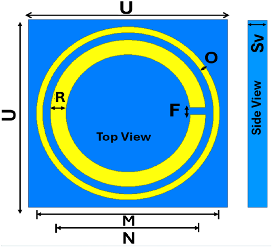
An analysis of the proposed FSS was conducted using Ansoft High Frequency Structure Simulator (HFSS). The unit cell, constructed on an Flame Retardant (FR-4) substrate, is illustrated in Figure 1.
Unit cell analysis of the proposed FSS corner reflector. Dimensions are U = 12, Sv = 1.20, O = 0.4, R = 1, M = 11.8, N = 10, and F = 0.5. All are in mm.

A patch-type FSS structure is adopted as a band-stop filter at the operating frequency range. Its operation was studied using the master–slave boundary analysis. The proposed unit cell consists of a circular ring and a slot ring having a slot-gap “F.” The electromagnetic behavior of metal split-ring electromagnetic structures is dominated by LC resonance: the metal ring provides inductance, while the gap introduces capacitance. Therefore, the resonance frequency of the unit cell can be approximated by:
 \begin{equation*}{f_r} = \frac{1}{{2\pi \sqrt {LC} }}\end{equation*}
where (L) and (C) represent the equivalent inductance and capacitance of the resonator, respectively. The FSS-based corner reflector unit independently developed in this study has geometric parameters that can significantly regulate its resonance response. The gap “F” modulates capacitance to shift the resonance band, the strip width “R” affects current distribution, the loop diameter “N” alters the inductance path and resonance frequency, and the parameter “M” acts on periodic coupling. These characteristics enable the unit to realize the preset target reflection response.
Figure 2(a) depicts the transmission characteristics and phase response of the proposed unit cell. It is demonstrated that the unit cell structure can achieve a deep transmission suppression with S21 < −28 dB together with a seamless 360° phase shift. This ensures that the phase difference is at a desirable value, with improved reflection characteristics. Thus, the proposed FSS at 5.1 GHz shows a good reflector, due to the robustness of the comparison capability plot and its noteworthy phase response.
(a) Transmission characteristics and reflection phase of the unit cell; and (b) transmission characteristics for different incident angles.

Figure 2 Long description
Two overlaid line plots sharing the same horizontal axis. The horizontal axis is labeled, Frequency (GHz), with tick labels at 4.0, 4.5 and 5.0. The left vertical axis is labeled, Transmission Coefficient (dB), ranging from 0 at the top down to minus 30 at the bottom, with tick labels at 0, minus 5, minus 10, minus 15, minus 20, minus 25 and minus 30. The right vertical axis is labeled, Reflection Phase (deg), ranging from minus 200 at the bottom to 200 at the top, with tick labels at minus 200, minus 150, minus 100, minus 50, 0, 50, 100, 150 and 200. One solid curve on the transmission axis decreases from about minus 10 decibel near 4.0 gigahertz to about minus 20 decibel near 4.5 gigahertz, then reaches about minus 30 decibel at about 5.0 gigahertz. A dashed curve on the reflection phase axis stays near about 100 degree around 4.0 gigahertz, then curves downward and reaches about minus 200 degree at about 5.0 gigahertz. A second solid curve on the reflection phase axis rises steeply just after 5.0 gigahertz, reaching about 200 degree, then slopes slightly downward toward about 150 degree by the right edge. The image B showing a line graph with multiple transmission curves. The horizontal axis is labeled, Frequency (GHz), with tick labels at 3, 4, 5, 6 and 7. The vertical axis is labeled, Transmission Coefficient (dB), ranging from 0 at the top down to minus 30 at the bottom, with tick labels at 0, minus 5, minus 10, minus 15, minus 20, minus 25 and minus 30. A legend lists four series: Theta 0 deg, Theta 30 deg, Theta 45 deg and Theta 60 deg. All four curves show a deep notch near 5 gigahertz. The Theta 0 deg curve is near about minus 2 decibel at 3 gigahertz, decreases to about minus 5 decibel near 4.5 gigahertz, drops to about minus 28 decibel near 5.0 gigahertz, then rises to about minus 3 decibel near 5.6 gigahertz and trends to about minus 6 decibel by 7 gigahertz. The Theta 30 deg curve follows a similar shape, reaching about minus 28 decibel near 5.0 gigahertz and then rising to around minus 4 decibel near 5.6 gigahertz before trending downward toward about minus 7 decibel by 7 gigahertz. The Theta 45 deg curve drops to about minus 28 decibel near 5.0 gigahertz and rises to around minus 5 decibel near 5.6 gigahertz, then trends to about minus 8 decibel by 7 gigahertz. The Theta 60 deg curve is lower than the others before the notch, reaching about minus 15 decibel near 4.5 gigahertz, drops to about minus 28 decibel near 5.0 gigahertz, then rises to around minus 6 decibel near 5.6 gigahertz and trends to about minus 10 decibel by 7 gigahertz.
Figure 2(b) presents the simulated S21 for different θ of the incident plane waves, indicating the excellent angular stability of the proposed FSS configuration. This angular stability is necessary for consistent reflection and different wave propagation characteristics, thus maintaining the reliable and reflective performance of the system in real-world applications.
The FSS array is formed utilizing the aforementioned unit cell as shown in Figure 3. These FSS screens serve as band-stop filters; they are of a concentric 4 × 4 disk unit cell, which is printed above an FR-4 substrate, as illustrated in Figure 3(a). Two arrays are employed to form a corner reflector placed over the ground, as shown in Figure 3(b). Moreover, the corner reflector has been shaped to maintain an angle of 90° between the two FSS planes for efficient reflection and radiation shaping.
Schematic diagram of the (a) FSS screens and (b) corner reflector (Lf = 48 mm).

Figure 3 Long description
Rectangular FSS screen drawn as a four by four array of repeated cells, where each cell contains one elliptical ring shape. A dimension line with arrowheads runs along the top edge and is labeled, Lf. A second dimension line with arrowheads runs along the left edge and is labeled, Lf. The subfigure label, left parenthesis a right parenthesis, appears near the upper right of this subfigure. Two rectangular FSS screens meeting along a vertical edge to form a corner shape. Each screen face shows the same repeated elliptical ring pattern across its surface. Dimension lines with arrowheads are drawn along the top edges and outer side edges of the two screens, each labeled, Lf. Near the bottom at the inside corner, the angle annotation reads, 90 degree. The subfigure label, left parenthesis b right parenthesis, appears near the lower right of this subfigure. The two subfigures present the same screen pattern as a single flat array in left parenthesis a right parenthesis and as two arrays joined at a right angle in left parenthesis b right parenthesis, with only the symbol Lf shown for dimensions and no numeric value or unit displayed.
E-field of antenna with corner reflector
This section examines the E-field distribution of the corner reflector with radiating elements. The role of the reflector in augmenting the directivity of antenna elements (CDRA) is clarified using image theory. Additionally, the ideal distance between the antenna configuration and the corner reflector is examined to attain optimal constructive interference and enhanced radiation efficacy.
Figure 4 illustrates the corner reflector integrated with the CDRA feed, accompanied by the corresponding E-field distribution. The E-field plot distinctly illustrates strong field confinement and reflection from the FSS surfaces, confirming the efficacy of the corner reflector in enhancing directivity.
3D structure of the antenna and its Cartesian coordinates.

Figure 4 Long description
A corner reflector integrated with a CDRA feed, showing the E-field distribution. At the top center is the observation point labeled L, connected by lines to various points on the structure. Two FSS reflectors are positioned at the bottom, labeled FSS Reflector1 on the right and FSS Reflector2 on the left. Between these reflectors, the CDRA Feed1 is located at the center bottom, marked with a label. Lines extend from the observation point to four points labeled s1, s2, s3 and s4, forming a triangular structure. The points s1 and s2 are connected to FSS Reflector1 and FSS Reflector2, respectively. The points s3 and s4 are connected to the CDRA Feed1. The diagram includes angles labeled theta and phi, with theta positioned near the top right and phi near the bottom right. Cartesian coordinates are marked with x, y and z axes, with x at the bottom left, y at the bottom right and z extending vertically from the observation point. The labels image2, image3 and image4 are positioned near s2, s3 and s4, respectively. The structure demonstrates strong field confinement and reflection from the FSS surfaces, enhancing directivity.
The resultant E-field (from the antenna [E 1] and its images [E 2–E 4]) at point P is plotted in Figure 4:
 \begin{align}{\text{ }}E\left( {s,\theta ,\varphi } \right) & = {E_1}\left( {{s_1},\theta ,\varphi } \right) + {\text{ }}{E_2}\left( {{s_2},{\text{ }}\theta ,\varphi } \right) + {\text{ }}{E_3}\left( {{s_3},\theta ,\varphi } \right) \\ \nonumber
& + {\text{ }}{E_4}\left( {{s_4},{\text{ }}\theta ,\varphi } \right)\end{align}
\noindent On the conducting surface of the FSS, which behaves as an equipotential surface, the tangential components of the incident and reflected E-fields must add up to zero:
 \begin{equation}{E_i} + {\text{ }}{E_r} = 0{\text{ }}or{\text{ }}{E_i} = - {E_r}\end{equation}
\noindent In the far-field zone, any radial spacing s 1 is defined as s 1 = s (for magnitude) and s 1 = s − mcosδ 1 (for phase). By applying the same principle to s 2–s 4, Equation (2) can be rewrite as
 \begin{align}E\left( {s,\theta ,\varphi } \right) &= \left[ {{{\text{e}}^{ - jmn\cos {\delta _1} - {\text{ }}}}{{\text{e}}^{ - jmn\cos {\delta _2} - {\text{ }}}}{{\text{e}}^{ - jmn\cos {\delta _3} - {\text{ }}}}{{\text{e}}^{ - jmn\cos {\delta _4} - {\text{ }}}}} \right] \nonumber\\
&\quad{}\times f\left( {\theta ,\varphi } \right)(\frac{{{e^{ - jns}}}}{s})\end{align}
\noindent Considering an isolated antenna element located at the origin Q that generates an E-field of magnitude E 0 at an arbitrary observation point L, the field relationship is formulated as follows:
 \begin{equation}\frac{E}{{{E_0}}} = 2[\cos \left( {nm\sin \theta \cos \varphi } \right) - {\text{cos}}(nm{\text{ }}sin\theta {\text{ }}sin\varphi )]\end{equation}
\noindent For the condition θ = 90° in the xy-plane and ϕ = 0° along the principal radiation direction, the expression can be reformulated in terms of the indices n and m as:
 \begin{equation}\frac{E}{{{E_0}}} = 2\left[ {\cos \left( {nm} \right) - 1} \right]\end{equation}
\noindent Now it is clear that any antenna with omnidirectional emission will have a gain increase in a particular direction when an FSS reflector is used. It is also evident from Equation (4) that the gain in the E-field changes as the space distance (m) changes and achieves its maximum for m = λ/2, 3λ/2, 5λ/2, 7λ/2, and so on. In the suggested design, the distance from the center of CDRA to the corner of the reflector should be kept at 25 mm for a half-wavelength perpendicular gap between the antenna and the FSS at 5.1 GHz.
Antenna with corner reflector
First, the single DRA structure without the FSS is examined, followed by the DRA integrated with the corner reflector. Figure 5 shows the geometry and dimensions of the proposed antenna. The dielectric resonator (DR-1), consisting of alumina ceramic material (ε DRA = 9.8), is positioned on the circular metallic plate. A coaxial probe is inserted at the center position of the resonator to excite it. Figure 5(b) shows the three-dimensional (3D) radiation pattern that demonstrates the TM01δ mode is excited in the DRA. This mode generates a monopole-like radiation pattern, which has omnidirectional properties in one plane. However, one significant disadvantage of these monopole-type antennas is their inherently low gain. Because modern wireless communication systems require high strength and directed radiation beams, further improvements are required.
Antenna geometry and 3D polar plot characteristics: (a) 3D view of the antenna with single DR elements; (b) 3D radiation pattern; and (c) radiation pattern in 2D (XY-plane).

Figure 5 Long description
A three-dimensional antenna geometry diagram. A circular plate is labeled, Ground. A cylindrical element on the plate is labeled, DR-1. A horizontal dimension across the cylinder is labeled, 30 millimeter, r. A vertical dimension on the cylinder is labeled, h 10 millimeter. A thickness label at the left reads, gt 1.6 millimeter. A horizontal dimension under the circular plate reads, Dg 72 millimeter. A small axis triad at upper left is labeled x, y, z. The image B showing a three-dimensional polar radiation plot with a vertical color scale bar beside it. The color scale bar is labeled from Max 2.0 at the top to Min minus 40.9 at the bottom, with tick labels 10, 0, minus 10, minus 20, minus 30, minus 40, minus 50. The plot is a rounded lobe centered in a spherical angle grid with degree markings around the perimeter. The image C showing a two-dimensional polar line plot with two traces and a legend. The legend lists Cross-Pol and Co-Pol. The radial axis label reads, Normalized Power, with unit, decibel. Radial tick labels shown are 0, minus 10, minus 20, minus 30, minus 40, minus 50, minus 60. Angle labels around the circle are 0, 30, 60, 90, 120, 150, 180, 210, 240, 270, 300, 330. The Co-Pol trace forms a near-circular ring close to the outer radius. The Cross-Pol trace forms a smaller multi-lobed shape nearer the center.
The structure of the DRA elements with a corner reflector is presented in Figure 6; it also shows the antenna’s reflection coefficient with and without the corner reflector. It reveals that the designed antenna resonates at 5.1 GHz.
(a) 3D image of the antenna and its Cartesian coordinates. (b) Simulated graph of reflection coefficients for the antenna with and without an FSS reflector. Dimensions are r = 30 mm, h = 10 mm, Dg = 72 mm, gt = 1.6 mm, Lf = 48 mm, and Wf = 1.2 mm.

Figure 6 Long description
A three dimensional antenna schematic. A patterned top surface shows repeated circular openings. A central cylindrical element is labeled DRA 1. A base is labeled Ground. Dimension arrows label r across the cylinder, h as the cylinder height, gt as a small vertical thickness at the base edge, Dg as a bottom width, Lf as a vertical side length and Wf as a top edge width. A Cartesian axis marker shows x, y and z. The image B showing a line graph with two curves and a legend. The x-axis label is Frequency, gigahertz, with tick labels 4.0, 4.2, 4.4, 4.6, 4.8, 5.0, 5.2 and 5.4. The y-axis label is S Parameters, decibel, with tick labels 0, minus 5, minus 10, minus 15, minus 20, minus 25 and minus 30. The legend lists without FSS and with FSS. The without FSS curve forms a broad dip, reaching about minus 17 decibel near 4.4 gigahertz, then rises toward about minus 2 decibel by 5.4 gigahertz. The with FSS curve stays near about minus 2 to minus 4 decibel from 4.0 to about 4.9 gigahertz, then drops to a narrow minimum near minus 30 decibel around 5.1 gigahertz and rises back to about minus 2 decibel by 5.4 gigahertz.
The 3D radiation pattern is depicted in Figure 7, showing the transformation of the radiation beam from an omnidirectional monopole-type pattern to a highly directed beam when the reflector is used. Without the corner reflector, the antenna has a gain of about 3 dB. The integration of the FSS-based corner reflector yields a significantly enhanced directional radiation pattern, achieving a peak gain exceeding 10 dB in the desired direction. This results in an overall gain improvement of roughly 209%. These findings clearly indicate the efficacy of the suggested reflector in improving directivity and radiation performance.
3D polar plot along with antenna structure: (a) 3D view and (b) front view.

Figure 7 Long description
A three-dimensional view of an antenna structure with a corner reflector. The reflector is depicted with a grid of circular elements on two perpendicular planes forming a corner. In front of the reflector, a large red spherical shape represents the radiation pattern, indicating high intensity. The base is green, suggesting lower intensity areas. The image B showing a front view of the same antenna structure. The corner reflector is visible with circular elements and the radiation pattern is again represented by a red spherical shape. An arrow extends from the center of the pattern, indicating the direction of the radiation beam. The base is green, similar to the previous view, indicating lower intensity areas. Both images include a color scale on the left, ranging from maximum 8.3 to minimum minus 24.4, representing the intensity levels.
Proposed four-port MIMO antenna: (a) 3D view and (b) side view.

Figure 8 Long description
The image consists of two parts. The first part, labeled as (a), shows a 3D view of a four-port MIMO antenna. It features four cylindrical dielectric resonator antennas (DRAs) labeled DRA-1, DRA-2, DRA-3 and DRA-4, positioned symmetrically on a circular green substrate. Two blue corner reflectors intersect at the center, forming an X shape. The second part, labeled as (b), presents a side view of the same antenna. It highlights the DRA-1 and DRA-2 on the green substrate, with a blue corner reflector featuring circular patterns. A legend on the right identifies the colors: orange for DRA, blue for substrate, green for ground and yellow for patch. The coordinate axes X, Y and Z are shown in the top left corner of the first part.
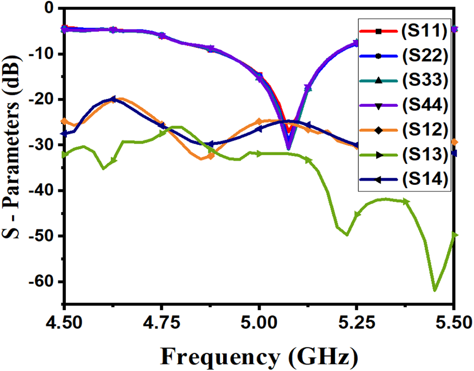
S-parameters of the presented four-port antennas.

Figure 9 Long description
S- Parameters (dB) The x-axis is labeled, Frequency (GHz), ranging from 4.50 to 5.50 with tick labels at 4.50, 4.75, 5.00, 5.25 and 5.50. The y-axis is labeled, S- Parameters (dB), ranging from 0 to minus 60 with tick labels at 0, minus 10, minus 20, minus 30, minus 40, minus 50 and minus 60. A legend lists seven series: (S11), (S22), (S33), (S44), (S12), (S13) and (S14). (S11) starts near minus 10 decibel at 4.50 gigahertz, rises to about minus 20 decibel near 4.65 gigahertz, then drops to about minus 30 decibel near 4.90 gigahertz. It rises to about minus 20 decibel near 5.05 gigahertz, then drops to about minus 30 decibel near 5.20 gigahertz and ends near minus 25 decibel at 5.50 gigahertz. (S22) starts near minus 10 decibel at 4.50 gigahertz, rises to about minus 20 decibel near 4.65 gigahertz, then drops to about minus 30 decibel near 4.90 gigahertz. It rises to about minus 20 decibel near 5.05 gigahertz, then drops to about minus 30 decibel near 5.20 gigahertz and ends near minus 25 decibel at 5.50 gigahertz. (S33) starts near minus 10 decibel at 4.50 gigahertz, rises to about minus 20 decibel near 4.65 gigahertz, then drops to about minus 30 decibel near 4.90 gigahertz. It rises to about minus 20 decibel near 5.05 gigahertz, then drops to about minus 30 decibel near 5.20 gigahertz and ends near minus 25 decibel at 5.50 gigahertz. (S44) starts near minus 10 decibel at 4.50 gigahertz, rises to about minus 20 decibel near 4.65 gigahertz, then drops to about minus 30 decibel near 4.90 gigahertz. It rises to about minus 20 decibel near 5.05 gigahertz, then drops to about minus 30 decibel near 5.20 gigahertz and ends near minus 25 decibel at 5.50 gigahertz. (S12) is near 0 decibel at 4.50 gigahertz, stays close to 0 decibel until about 4.80 gigahertz, then slopes downward to about minus 10 decibel near 5.00 gigahertz. It reaches about minus 30 decibel near 5.20 gigahertz, then rises slightly and ends near minus 20 decibel at 5.50 gigahertz. (S13) is near minus 25 decibel at 4.50 gigahertz, rises to about minus 20 decibel near 4.65 gigahertz, then drops to about minus 30 decibel near 4.85 gigahertz. It stays near minus 30 decibel until about 5.15 gigahertz, then drops to about minus 50 decibel near 5.25 gigahertz, rises to about minus 40 decibel near 5.35 gigahertz and ends near minus 55 decibel at 5.50 gigahertz. (S14) is near minus 30 decibel at 4.50 gigahertz, rises to about minus 25 decibel near 4.70 gigahertz, then drops to about minus 30 decibel near 4.90 gigahertz. It stays near minus 30 decibel until about 5.15 gigahertz, then drops to about minus 45 decibel near 5.25 gigahertz, rises to about minus 35 decibel near 5.35 gigahertz and ends near minus 50 decibel at 5.50 gigahertz.
3D polar plot of the proposed antenna for different ports.

Figure 10 Long description
The plot displays radiation patterns for four DRA elements labeled DRA-1, DRA-2, DRA-3 and DRA-4. Each pattern is shown in a circular plot surrounding a central diagram. The color scale on the left indicates gain in decibels, ranging from minus 35 to 10. The central diagram shows the arrangement of the DRA elements. Each polar plot represents the radiation pattern for one element, with main lobes oriented in different directions. DRA-1 shows a main lobe directed toward the bottom, DRA-2 toward the right, DRA-3 toward the top and DRA-4 toward the left. The plots illustrate multidirectional radiation, contributing to pattern diversity and reduced mutual coupling. The color scale provides a visual representation of gain, with red indicating higher gain and blue indicating lower gain.
After attaining satisfactory results with the single-port DRA element, the design was expanded to include four ports. To do this, an additional corner reflector was added, resulting in four unique corner segments. CDRAs were carefully located λ/2 away from each corner of the reflector. This configuration forms a four-port MIMO antenna system in accordance with the one that effectively utilizes the reflector for improved radiation performance. The orientation of the designed antenna is illustrated in Figure 8, in which four CDRAs are unified with the FSS-based corner reflector. The S-parameters of the proposed MIMO antenna are shown in Figure 9. Due to symmetric orientation, the reflection coefficient for all the ports is almost the same. Figure 9 additionally illustrates the isolation characteristics of the proposed antenna, revealing values over 20 dB for all port combinations. The cause of the significant isolation is apparent from the 3D polar plot presented in Figure 10. The four DR elements radiate in four unique directions, hence creating multidirectional pattern diversity. This pattern diversity significantly reduces mutual coupling among the antenna elements, leading to high isolation performance.
Experimental results
The suggested quad-port MIMO antenna was successfully constructed and experimentally evaluated. This study designs measurement workflows for two categories of core radio frequency (RF) parameters. For S-parameters including reflection coefficient and port isolation, the Rohde & Schwarz ZNB20 vector network analyzer is adopted; a full SOLT calibration is completed prior to measurement, and all idle ports are connected to 50 Ω matching loads. For measurements of biplanar far-field radiation patterns, a standard-gain horn and a power meter fitted with a power sensor are used to receive signals, while the same ZNB20 unit serves as the continuous-wave source. Figure 11 illustrates the top and side perspectives of the constructed prototype, whilst the recorded S-parameters and gain plot are depicted in Figure 12. It also shows that a strong correlation between simulated and measured results is evident, confirming the design’s correctness. Without the presence of the reflector, the antenna demonstrates a gain of roughly 3 dB. The inclusion of the corner reflector results in a gain of around 9.9 dB, signifying an enhancement of nearly 209%, as depicted in Figure 12(b).
Pictures of the proposed antenna from the (a) side and (b) top.

Experimental outcome of the proposed antenna: (a) S-parameters; and (b) gain plot.

Figure 12 Long description
A line graph with the y axis labeled, S parameters in decibel, ranging from negative 60 to 0 and the x axis labeled, Frequency in gigahertz, ranging from 4.50 to 5.50. A legend lists S11, S22, S33, S44, S12, S13 and S14. The plotted lines show multiple dips between about 4.70 and 5.35 on the frequency axis, with the lowest dip reaching about negative 40 on the S parameters axis. The image B showing a line graph with the y axis labeled, Peak Gain in decibel, ranging from 0 to 10 and the x axis labeled, Frequency in gigahertz, ranging from 4.50 to 5.50. A legend lists with FSS s, with FSS m and without FSS. The with FSS s series has points near 7 at 4.50, near 9 at 4.90, near 9 at 5.00, near 10 at 5.20 and near 10 at 5.30. The with FSS m series has points near 9 at 5.00, near 9 at 5.10, near 9 at 5.20 and near 9 at 5.30. The without FSS series has points near 4 at 4.50, near 4 at 4.70, near 4.5 at 4.90, near 5 at 5.10, near 5 at 5.20 and near 5 at 5.30.
Figure 13 displays the proposed quad-port MIMO antenna’s 2D radiation pattern in the XY-plane. The DR element radiates in a different direction, as can be shown in Figure 13. Without a reflector, the DR elements create an omnidirectional radiation pattern in the XY-plane, as shown in Figure 5(c). But, to ensure directed radiation from each port, DRA-1 to DRA-4 is specifically excited along ϕ = 135°, 225°, 315°, and 45°, respectively. This behavior is confirmed by the 3D polar plot presented in Figure 10, which substantiates the antenna’s multidirectional radiation and pattern diversity.
Simulated (S) and measured (M) 2D radiation pattern at 5.1 GHz in the XY-plane.

Figure 13 Long description
Four polar plots arranged in a two by two grid, labeled DRA 1, DRA 2, DRA 3 and DRA 4. Each plot has a circular angle scale marked 0, 30, 60, 90, 120, 150, 180, 210, 240, 270, 300 and 330. Each plot has a radial axis labeled, Normalised Power, with unit, decibel and radial tick labels 0, minus 10, minus 20 and minus 30. Each plot includes a legend with four entries: Co Pol (S), Co Pol (M), X Pol (S) and X Pol (M). Top left plot labeled DRA 1. The Co Pol (S) trace forms a broad lobe with its largest radius around angles near 120 to 150 and smaller lobes around other angles. The Co Pol (M) trace forms a broad lobe with its largest radius around angles near 120 to 150. The X Pol (S) trace forms multiple smaller lobes around the circle, with the largest radii around angles near 0 to 60 and near 300 to 330. The X Pol (M) trace forms multiple smaller lobes, with larger radii around angles near 0 to 60 and near 300 to 330. Top right plot labeled DRA 2. The Co Pol (S) trace has a broad lobe with the largest radius around angles near 210 to 270 and a smaller lobe around angles near 30 to 90. The Co Pol (M) trace has a broad lobe with the largest radius around angles near 210 to 270. The X Pol (S) trace shows multiple smaller lobes, with larger radii around angles near 0 to 60 and near 300 to 330. The X Pol (M) trace shows multiple smaller lobes, with larger radii around angles near 0 to 60 and near 300 to 330. Bottom left plot labeled DRA 3. The Co Pol (S) trace has a broad lobe with the largest radius around angles near 300 to 30 and another broad lobe around angles near 180 to 240. The Co Pol (M) trace has a broad lobe with the largest radius around angles near 300 to 30. The X Pol (S) trace forms multiple smaller lobes, with larger radii around angles near 0 to 60 and near 240 to 300. The X Pol (M) trace forms multiple smaller lobes, with larger radii around angles near 0 to 60 and near 240 to 300. Bottom right plot labeled DRA 4. The Co Pol (S) trace has a broad lobe with the largest radius around angles near 90 to 150 and another broad lobe around angles near 240 to 300. The Co Pol (M) trace has a broad lobe with the largest radius around angles near 90 to 150. The X Pol (S) trace shows multiple smaller lobes, with larger radii around angles near 0 to 60 and near 300 to 330. The X Pol (M) trace shows multiple smaller lobes, with larger radii around angles near 0 to 60 and near 300 to 330.
Table 1 in this paper lists the simulation performance of four DRA configurations, covering three performance metrics: gain (dBi), half-power beamwidth (HPBW), and front-to-back ratio (F/B). For all metrics, control scenarios were set up to compare cases with a reflector plate added against cases without a reflector plate. Test results show that across all four designs, adding a reflector plate can significantly improve gain and F/B, while substantially narrowing the beamwidth.
Comparison results of simulated and measured parameters with and without reflector

Table 1 Long description
Simulated and measured values are listed for gain in dBi, HPBW in degrees, and F over B ratio in dB for DRA 1 through DRA 4, each reported without reflector and with reflector. For DRA 1, without reflector gives gain 3.2 simulated and 3.05 measured, HPBW 89.3 simulated and 89.11 measured, and F over B ratio 12.3 simulated and 12.15 measured; with reflector gives gain 9.72 simulated and 8.73 measured, HPBW 38.58 simulated and 38.45 measured, and F over B ratio 15.4 simulated and 15.32 measured. For DRA 2, without reflector gives gain 3.58 simulated and 3.41 measured, HPBW 92.72 simulated and 91.87 measured, and F over B ratio 10.62 simulated and 9.98 measured; with reflector gives gain 9.85 simulated and 8.61 measured, HPBW 56.12 simulated and 55.78 measured, and F over B ratio 13.03 simulated and 12.87 measured. For DRA 3, without reflector gives gain 3.4 simulated and 3.31 measured, HPBW 91.38 simulated and 90.89 measured, and F over B ratio 10.89 simulated and 10.56 measured; with reflector gives gain 9.9 simulated and 8.97 measured, HPBW 55.89 simulated and 55.81 measured, and F over B ratio 13.72 simulated and 12.61 measured. For DRA 4, without reflector gives gain 3.58 simulated and 3.53 measured, HPBW 88.14 simulated and 87.89 measured, and F over B ratio 11.27 simulated and 11.14 measured; with reflector gives gain 9.85 simulated and 8.61 measured, HPBW 34.75 simulated and 34.56 measured, and F over B ratio 14.31 simulated and 13.98 measured. Across all four DRAs, the with reflector rows show higher gain and higher F over B ratio than the without reflector rows, while HPBW is lower with reflector than without reflector in both simulation and measurement.
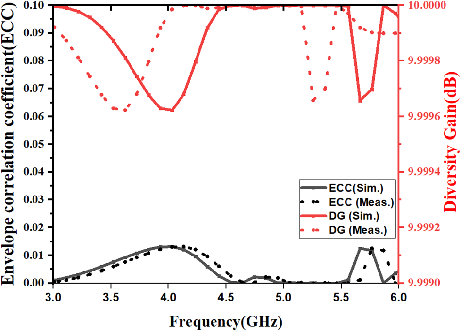
The simulated/measured Envelop Corellation Coefficient (ECC) and Diversity Gain (DG) within the operating frequency band are presented in Figure 14. It is observed that ECC remains well below 0.1 throughout the entire frequency range, with a minimum value approaching zero, indicating excellent isolation and low correlation between the antenna ports. In addition, the antenna maintains a stable directivity gain of approximately 10 dBi across the operating band. The close agreement between the simulated and measured results further validates the effectiveness and reliability of the proposed antenna design.
Simulated and measured ECC and diversity gain.

Figure 14 Long description
Envelope correlation coefficient and diversity gain. The x-axis is labeled, Frequency gigahertz, ranging from 3.0 to 6.0 in increments of 0.5. The left y-axis is labeled, Envelope correlation coefficient, ranging from 0.00 to 0.10 in increments of 0.01. The right y-axis is labeled, Diversity gain decibel, ranging from 9.9900 to 10.0000 in increments of 0.0020. A legend inside the plot lists four series: ECC sim, ECC meas, DG sim and DG meas. Two black curves plot envelope correlation coefficient. The solid black curve starts near 0.01 at 3.0, rises to about 0.02 around 4.0, then declines toward about 0.01 by about 5.0. It then rises to a small peak near about 0.03 around 5.6, drops back near about 0.01 around 5.8 and ends near about 0.02 at 6.0. The dashed black curve follows a similar shape, staying close to the solid black curve, with a small peak near about 0.03 around 5.6. Two red curves plot diversity gain. The solid red curve is near 10.0000 at 3.0, dips to about 9.996 around 3.8 to 4.0, then rises back near 10.0000 by about 4.6 and stays near 10.0000 until about 5.5. It then drops sharply to about 9.992 around 5.7 and rises again toward about 10.0000 by about 5.9 to 6.0. The dashed red curve stays close to 10.0000 for most of the range, with a dip near about 9.996 around 3.8 to 4.0 and a sharp dip near about 9.992 around 5.7.
Comparative performance of the proposed antenna with existing MIMO antennas

Table 2 Long description
Columns list Ref., No. of ports, Isolation Level, Isolation Techniques, and Multi Directional Pattern. Four entries are compared, and each has 4 ports. Ref. [8] lists isolation level 20 dB with metamaterial and multi directional pattern, No. Ref. [12] lists 22 dB with FSS and multi directional pattern, Yes. Ref. [19] lists 20 dB with spatial placement and multi directional pattern, Yes. This Work lists 26 dB with corner reflector and multi directional pattern, Yes.
Table 2 shows a comparative analysis of the performance between the proposed antenna and other relevant published studies. The comparative analysis has been conducted regarding the number of ports, isolation level, mutual coupling reduction approaches, and pattern diversity capability. Table 2 demonstrates that the suggested design attains high isolation and increased pattern variety while supporting a greater number of ports than the referred antennas.
Conclusion
A quad-port MIMO CDRA using FSS corner reflectors has been designed and experimentally demonstrated. A four-port arrangement was developed, achieving isolation exceeding 20 dB, improved directivity, and multidirectional pattern diversity. The proposed concept is highly appropriate for higher-generation MIMO wireless communication systems.
Funding statement
This research received no specific grant from any funding agency, commercial, or not-for-profit sectors.
Competing interests
The authors report no conflict of interest.

Ankit Mayur obtained the Bachelor of Technology degree from Veer Bahadur Singh Purvanchal University, Jaunpur, Uttar Pradesh, India, in 2012, and the Master of Technology degree from Sam Higginbottom University of Agriculture, Technology and Sciences (SHUATS), Prayagraj, Uttar Pradesh, India, in 2014. He is currently pursuing the Ph.D. degree in RF and Microwave Engineering with the Department of Electronics and Communication Engineering, Motilal Nehru National Institute of Technology (MNNIT) Allahabad, Prayagraj, India. His current research interests include DRAs, FSS, beam-tilt featured antennas, beam-steering antennas, reconfigurable antennas, MIMO antennas, circularly polarized antennas, and antennas for IoT applications.

Abhimanyu Yadav received the B.Tech. degree in Electronics and Communication Engineering in 2016, the M.Tech. degree in Digital Systems from MNNIT Allahabad, India, in 2019, and the Ph.D. degree from MNNIT Allahabad in 2025. His doctoral research focused on the design and development of dielectric-resonator-based filtering antennas for wireless applications. He is currently associated with Galgotias University, Greater Noida, India. His research interests include RF and microwave engineering, DRAs, MIMO antennas, metasurfaces, filtering antennas, electromagnetic wave propagation, and analog and digital circuit design. He has authored and co-authored several research articles in international journals and conferences.

Gourab Das was born in Radhamohanpur (West Bengal), India, in 1990. He completed his B.Tech. in Electronics and Communication Engineering from West Bengal University of Technology, Kolkata, India, in 2012 and M.Tech. in ECE from Indian Institute of Technology (Indian School of Mines), Dhanbad, India. He completed his Ph.D. from Indian Institute of Technology (Indian School of Mines), Dhanbad, India in 2020. Currently, Dr Das is working as an Assistant Professor in the Department of Electronics & Communication Engineering at Punjab Engineering College (Deemed to be University) Chandigarh. Prior to joining PEC Chandigarh, he worked as a Postdoctoral Fellow at IIT Kanpur. He has authored or co-authored over 50 research papers in international/national journals/conference proceedings. He has received the Best Research Publication Award – 2019 organized by Electronics Engineering Department of IIT (ISM) Dhanbad. His research interests include DRA, antenna array, and MIMO antenna.

Anand Sharma obtained a Bachelor of Technology from Uttar Pradesh Technical University Lucknow, in 2012, a Master of Technology from Jaypee University of Engineering and Technology Guna, in 2014, and a Ph.D. in RF and Microwave from Indian Institute of Technology (ISM), Dhanbad, in 2018. After that, he joined Government Engineering College Sonbhadra, Uttar Pradesh, as an Assistant Professor in the Electronics Engineering Department and left the college in June 2019. Currently, he holds the position of Assistant Professor in the Department of Electronics and Communication Engineering, Motilal Nehru National Institute of Technology Allahabad, Prayagraj, Uttar Pradesh, India. He has published more than 60 articles in international journals (SCI-Indexed) and has also presented more than 40 articles at national/international conferences. His area of research includes MIMO antennas, antennas for IoT applications, circularly polarized DRAs, ultra-wideband and super-wideband antennas, wearable antennas, and antenna optimization using machine learning.