1 INTRODUCTION
The vast majority of the empirical asset pricing literature works with standard time-series linear factor models in which the dependent variable represents the excess return of a stock or a portfolio and the independent variables represent spreads of certain factor portfolios (Fama and French, Reference Fama and French1992, Reference Fama and French2015, Reference Fama and French2020; Carhart, Reference Carhart1997). There is a large strand of literature on identification of factors (Harvey, Liu, and Zhu, Reference Harvey, Liu and Zhu2016; Hou, Xue, and Zhang, Reference Hou, Xue and Zhang2020) and the econometric problem of estimation and testing of linear factor models (Jagannathan and Wang, Reference Jagannathan and Wang1996; Feng, Giglio, and Xiu, Reference Feng, Giglio and Xiu2020). Even though the linear time-series regression model is typically not tested for adequacy in this strand of literature, it has become a de facto standard and is widely regarded as a useful framework.
In this article, an asymptotic probabilistic argument is developed which can explain why linear models can be adequate in time-series regressions of variables that represent financial returns. The argument is based on the idea that lower frequency logarithmic returns can be viewed as temporally aggregated higher frequency returns. In particular, we prove that if the data generating process belongs to the class of Lévy processes—a fundamental building block in the field of finance (Rachev and Mittnik, Reference Rachev and Mittnik2000; Cont and Tankov, Reference Cont and Tankov2003)—the corresponding conditional expectation converges to a linear function as the return frequency declines. Furthermore, the rate of convergence is proved to be bounded by a power law with an exponent determined by certain joint moment conditions with econometric content.
The main result is presented first assuming bounded second moments justified by the theoretical and practical significance of this assumption. We demonstrate that the moment conditions determining the exponent of the power law are related to the first-order conditions of a specific least-squares problem. In addition, we show that when the dependent variable is a portfolio return, the rate of convergence can benefit from the cross-sectional aggregation of the individual stock returns. That is, linear models can be more adequate on a relative basis for portfolios rather than individual stocks for a given return frequency under the assumptions in the article. This is an important insight of both theoretical and practical significance for applications in finance.
Relaxing the assumptions of finite second moments leads to a number of difficulties mainly because the conditional expectation of the aggregated process may converge to a nonlinear function. We develop two rate-of-convergence results in this setting. First, the finite variance result is extended assuming conditions that guarantee linearity of the conditional expectation of the corresponding limiting stable law. In this formulation, the stable law appears explicitly in the new moment conditions and its tail index affects the rate of convergence in the limit theorem. Second, these assumptions are relaxed and the rate of convergence to the corresponding nonlinear function is derived. In this general situation, the associated moment conditions are very similar to the ones behind modern rate-of-convergence results in the generalized central limit theorem (GCLT).
The approach developed in the article connects two unrelated fields. On the one hand, it is related to model adequacy testing in the econometric literature because we take advantage of some aspects of the fundamental work by Bierens (Reference Bierens1982, Reference Bierens2016). Even though constructing an adequacy test is not a focus of this work, effectively new functionals measuring neglected nonlinearity are developed, which are also suitable for studying a rate-of-convergence problem. Separately, the results in this article can be viewed as an analytic confirmation of the observation made by Granger and Lee (Reference Granger and Lee1999) in a Monte Carlo study that linear models can become more adequate on a relative basis for aggregated data.
On the other hand, our approach is related to the probability metrics literature. From the point of view of probability theory, determining the rate of convergence in a limit theorem is best handled by functionals with certain metric properties. The metric approach has been used to address such questions in the central limit theorem (CLT) and the GCLT (Zolotarev, Reference Zolotarev2011; Rachev et al., Reference Rachev, Klebanov, Stoyanov and Fabozzi2013). The functionals constructed in this article borrow from that theory to establish the general stability of linear models and their domain of attraction in the context of Lévy processes. More generally, the main results can be restated without modification for the classical GCLT scheme of sums of independent and identically distributed (i.i.d.) random vectors.
An unexpected result in the article is that the moment conditions determining the rate of convergence do not include the marginals of the joint multivariate process. This is in contrast to similar moment conditions in the GCLT setting. An explanation for the weaker form of these conditions is that the research problem involves distances between conditional expectations rather than probability laws. As a consequence of the weaker conditions, the rate of convergence to a linear conditional mean can be faster than the rate of convergence in the associated GCLT indicating that the results in this article can be viewed as a separate class of limit theorems specialized for conditional means.
Even though the intended application is finance, the results in the article can be relevant for other domains where temporal and cross-sectional data aggregation are natural. For instance, important variables in macroeconomics, such as production, profits, employment, or consumption, are measured as sums of quantities observed for firms or families, which is an example of cross-sectional aggregation (Granger, Reference Granger1987). Some variables in economics are sums of flows over time and are sampled systematically at lower time frequencies leading to temporal aggregation. Examples include stock variables such as wealth and flow variables such as sales or production (Granger and Lee, Reference Granger and Lee1999). Apart from the field of finance, linear models play a fundamental role in economics as well (Stock and Watson, Reference Stock, Watson, Clements and Hendry2011) and their adequacy may be affected by the degree of data aggregation.
The article is organized in the following way. Section 2 defines the problem, clarifies the connection with model adequacy testing in the econometric literature, and develops a motivating example. Section 3 establishes a rate-of-convergence result assuming the existence of second moments and discusses the combination of cross-sectional and temporal aggregation. Section 4 develops the infinite variance case and comments on the connection with the classical rate-of-convergence results in the GCLT setting. Section 5 provides numerical examples and discusses further extensions of the theory. Finally, Section 6 concludes. The proofs of all lemmas and theorems are provided in the Appendix.
2 MEASURING NEGLECTED NONLINEARITY
In the empirical asset pricing literature, it is common to estimate and test asset pricing models using a linear time-series regression in which the dependent variable
 $Y_t \in \mathbb {R}$
is represented by the return of a portfolio of risky assets and the independent variables
 $X_t \in \mathbb {R}^d$
represent returns of factor replicating portfolios. It is common to use monthly returns for model estimation.
Logarithmic returns have a temporal aggregation property. Monthly log-returns can be computed as a sum of daily log-returns and, in this sense, they can be viewed as temporally aggregated daily returns. More generally, log-returns at any frequency can be represented as temporally aggregated higher frequency returns at some fixed frequency of observation. Even though not formally analyzed in this way, a decision to work with lower frequencies can be regarded as a decision to take advantage of temporal aggregation. In this article, we argue that the functional form of the conditional expectation
 $\mathbb {E}[Y_t|X_t]$
can become asymptotically linear as the degree of temporal aggregation increases and we study the rate of convergence in the limit problem.
In a broader non-financial context, Granger and Lee (Reference Granger and Lee1999) argue that many series in economics may be generated at one time interval but observed at another, greater time interval. For example, many variables are systematically sampled quarterly and each quarterly data point is a sum of the observations generated within the quarter. This process leads to temporally aggregated data at the quarterly frequency. In a Monte Carlo simulation, the authors conclude that temporal aggregation can simplify nonlinearity.
To address questions about the asymptotic behavior of
 $\mathbb {E}[Y_t|X_t]$
, we need a functional that meets the next two general conditions:
-
(a) The functional has the capacity to measure model misspecification.
-
(b) The functional is suitable to study rate-of-convergence problems.
Concerning the first condition, measuring neglected nonlinearity is a special case of the more general problem of measuring the degree of misspecification in nonlinear models. Fundamental results due to Bierens (Reference Bierens1982) establish necessary and sufficient conditions for a model to be correctly specified. Consider the following specification:
 $$ \begin{align} Y_t = m(X_t, \theta) + \epsilon_t, \end{align} $$
where
 $\theta $
is a vector of parameters,
 $m(x, \theta )$
is a nonlinear function, and
 $\epsilon _t$
is a residual. The model in (1) is said to be correctly specified if
 $\mathbb {E}[\epsilon _t|X_t] = 0$
almost surely, which guarantees that
 $\mathbb {E}[Y_t|X_t] = m(X_t,\theta )$
in the almost sure sense. The necessary and sufficient conditions are given by
 $$ \begin{align} \mathbb{E}\epsilon_t e^{i u^{\mathsf{T}} X_t} = 0,\quad \forall u \in \mathbb{R}^d, \end{align} $$
where
 $i = \sqrt {-1}$
denotes the imaginary unit.
In the econometric literature, moment conditions of the type presented in equation (2) are the foundation of integrated conditional moment tests employed to test for model adequacy. Bierens and Ploberger (Reference Bierens and Ploberger1997) develop asymptotic theory for tests based on the following functional:
 $$ \begin{align} \eta(\theta) = \int_{K}\left|\mathbb{E}\epsilon_tw(u^{\mathsf{T}} \Phi(X_t))\right|^2d\mu(u), \end{align} $$
where
 $\epsilon _t$
is the residual in (1),
 $w(z)\colon \mathbb {C}\rightarrow \mathbb {C}$
is a weighting function assumed to be analytic,
 $\Phi $
is a bounded one-to-one mapping, and
 $\mu (u)$
is a probability measure absolutely continuous with respect to the Lebesgue measure on a compact
 $K \subset \mathbb {R}^d$
. A test for model adequacy is based on the result that if
 $\mathbb {E}[\epsilon _tw(u^{\mathsf {T}} \Phi (X_t))] = 0$
for some
 $\theta _0 \in \Theta $
and all
 $u \in \mathbb {R}^d$
, or equivalently if
 $\eta (\theta _0) = 0$
, then
 $\mathbb {E}[\epsilon _t|X_t] = 0$
almost surely. The conditions in (2) arise with the exponential weights
 $w(z) = e^{iz}$
.
Other weighting functions have also been considered. If we generalize the notation to
 $w(X_t, u)$
, then notable alternatives to the exponential function include the indicator function
 $w(X_t,u) = 1_{\{X_t \leq u\}}$
proposed by Stute (Reference Stute1997) and other alternatives, such as
 $w(X_t,u) = \sin (u^{\mathsf {T}} X_t)$
or
 $w(X_t,u) = 1/(1+\exp (c-u^{\mathsf {T}} X_t))$
suggested by Stinchcombe and White (Reference Stinchcombe and White1998), and
 $w(X_t,u) = 1_{\{\beta ^{\mathsf {T}} X_t \leq u\}}$
suggested by Escanciano (Reference Escanciano2006) in which
 $\beta $
is assumed to be on the unit sphere in
 $\mathbb {R}^d$
and the integration in equation (3) is extended appropriately. It is worth noting that different weighting function families lead to a different power of the test, as emphasized in the literature.
Regarding the two properties mentioned earlier, any member of the family in equation (3), possibly extended with a more general weighting function, meets the criterion in (a). Unfortunately, no member of the extended family appears suitable as far as the criterion in (b) is concerned, which we illustrate further below.
Since our research question involves aggregation across time, we need an assumption about the underlying stochastic process. We assume that the vector of the dependent and the independent variables
 $\{V_t = (Y_t, X_t), t> 0\}$
follows a Lévy process, which represents a common assumption in mathematical finance (Rachev and Mittnik, Reference Rachev and Mittnik2000; Cont and Tankov, Reference Cont and Tankov2003). More formally,
 $V_t$
is a multivariate Lévy process if (Sato, Reference Sato1999):
-
1.
 $V_0 = 0$
almost surely.
-
2.
$V_t$
has independent increments; that is, for any choice of n and
$0 \leq t_0 < t_1 < \cdots < t_n$
, the random vectors
$V_{t_0}, V_{t_1} - V_{t_0},\ldots , V_{t_n} - V_{t_{n-1}}$
are independent. -
3. The distribution of
$V_{s+t} - V_s$
does not depend on s. -
4. The process is stochastically continuous and its sample paths are right-continuous with left limits.





Consider n intervals of equal fixed length
 $\Delta t$
and calculate the increments of the process
 $\Delta V_k = V_{t_k} - V_{t_{k-1}}$
,
 $k = 1,\ldots , n$
, where
 $t_{k} - t_{k-1} = \Delta t$
. From the standpoint of applications,
 $n\Delta t$
can be interpreted as the sampling frequency while the fixed
 $\Delta t$
stands for the frequency at which the series is generated. The process at time
 $n\Delta t$
can be represented as a sum of increments
 $$\begin{align*}V_{n\Delta t} = (Y_{n\Delta t}, X_{n\Delta t}) = \left(\sum_{k = 1}^n\Delta Y_{k}, \sum_{k = 1}^n\Delta X_{k}\right), \end{align*}$$
which are i.i.d. Even though the conditional mean
 $\mathbb {E}[Y_{\Delta t}|X_{\Delta t}]$
can be arbitrary, in this article, we show that the conditional mean
 $\mathbb {E}[Y_{n\Delta t}| X_{n\Delta t}]$
is approximately linear for large n.Footnote
1
Next, we demonstrate that the expectation in equation (2) indeed decays for the aggregated process where, without loss of generality, we assume that
 $\mathbb {E}(V_t) = 0$
. We note that the question for the asymptotic behavior of the conditional mean of
 $V_{n\Delta t}$
makes sense only if the limiting distribution of the random vector is non-degenerate, and to this end, the corresponding sums need to be normalized. For this demonstration, we assume that all second-order moments of
 $V_t$
are bounded. The needed normalization is then provided by
 $n^{-1/2}$
. Additionally, the least-squares estimator denoted by
 $$ \begin{align} \theta^* = (\mathbb{E}[X_{\Delta t}X_{\Delta t}^{\mathsf{T}}])^{-1}\mathbb{E}[Y_{\Delta t}X_{\Delta t}] \end{align} $$
is assumed to exist, and the expectation in equation (2) corresponding to a linear specification
 $m(X_{n\Delta t}, \theta ) = X_{n\Delta t}^{\mathsf {T}}\theta $
as a function of n is denoted by
 $$ \begin{align*} \varpi_n(u) = \mathbb{E}\left(n^{-1/2}(Y_{n\Delta t} - X_{n\Delta t}^{\mathsf{T}}\theta)e^{iu^{\mathsf{T}} n^{-1/2}X_{n\Delta t}}\right) \end{align*} $$
after normalizing
 $V_{n\Delta t}$
by
 $n^{-1/2}$
. If the linear specification is asymptotically correct, then
 $\varpi _n(u)$
with
 $\theta = \theta ^*$
must decay for all u.
By the independence of the increments,
 $\theta ^*$
is the same for each individual increment and also for their sum. The expectation in
 $\varpi _n(u)$
can be decomposed in the following manner:
 $$ \begin{align}\nonumber \varpi_n(u) &= \mathbb{E}\left(n^{-1/2}(Y_{n\Delta t} - X_{n\Delta t}^{\mathsf{T}} \theta^*)e^{iu^{\mathsf{T}} n^{-1/2}X_{n\Delta t}}\right)\\\nonumber &= n^{-1/2}\sum_{k = 1}^n\mathbb{E}\left[(\Delta Y_{k} - \Delta X_{k}^{\mathsf{T}} \theta^*)e^{i(n^{-1/2}u)^{\mathsf{T}} \sum_{j = 1}^n\Delta X_{j}}\right]\\\nonumber &= n^{-1/2}\sum_{k = 1}^n\mathbb{E}\left[(\Delta Y_{k} - \Delta X_{k}^{\mathsf{T}} \theta^*)e^{i(n^{-1/2}u)^{\mathsf{T}} \Delta X_{k}}\right]\mathbb{E}\left[e^{i(n^{-1/2}u)^{\mathsf{T}} \sum_{j \not = k}\Delta X_{j}}\right]\\ &= n^{1/2}\varpi_1(n^{-1/2}u)\left[\phi_{X_{\Delta t}}(n^{-1/2}u)\right]^{n-1}, \end{align} $$
where
 $\phi _{X_{\Delta t}}(u)$
is the characteristic function (ch.f.) of
 $X_{\Delta t}$
. Equation (5) indicates that the rate of decay of the left side for a fixed u is essentially determined by the rate of decay of
 $\sqrt {n}\varpi _1(u/\sqrt {n})$
because under the assumption of finite variance
 $$\begin{align*}\left[\phi_{X_{\Delta t}}(n^{-1/2}u)\right]^{n-1} \rightarrow e^{-\frac{1}{2}u^{\mathsf{T}} \mathbf{C} u}, \end{align*}$$
where
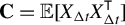 $\mathbf {C} = \mathbb {E}[X_{\Delta t}X_{\Delta t}^{\mathsf {T}}]$
. Thus, to understand the behavior of the right side of (5), we employ the Taylor series expansion at
 $u = 0$
,
 $$ \begin{align} n^{1/2}\varpi_1(n^{-1/2}u) &= n^{1/2}\varpi_1(0) + \sum_{j = 1}^d\frac{\partial \varpi_1({0})}{\partial u_{j}}u_{j} + \mathrm{o}(n^{-1/2}\left\lVert u\right\rVert_2)\\\nonumber &= n^{1/2}\mathbb{E}[\epsilon_{\Delta t}] + i u^{\mathsf{T}} \mathbb{E}[\epsilon_{\Delta t} X_{\Delta t}] + \mathrm{o}(n^{-1/2}\left\lVert u\right\rVert_2) \\\nonumber &= \mathrm{o}(n^{-1/2}\left\lVert u\right\rVert_2), \end{align} $$
where the last equality holds because
 $\mathbb {E}[\epsilon _{\Delta t}] = 0$
and
 $\mathbb {E}[\epsilon _{\Delta t} X_{\Delta t}] = 0$
from the first-order conditions of the least-squares problem. The required smoothness of
 $\varpi _1(u)$
follows from the assumed existence of the second moment of the process
 $V_t$
.
Indeed,
 $\varpi _n(u)$
converges to zero asymptotically for any fixed
 $u \in \mathbb {R}^d$
by a classical CLT argument and, as a result,
 $\mathbb {E}[Y_{n\Delta t}| X_{n\Delta t}]$
converges almost surely to a linear function. That is, the specification
 $$ \begin{align*} Y_t = X_t^{\mathsf{T}}\theta + \epsilon_t \end{align*} $$
with
 $\theta = \theta ^*$
becomes asymptotically correct for large t. Concerning the choice of functional mentioned earlier, consider again
 $\eta (\theta )$
in equation (3). In view of the steps needed to derive (5), clearly the only possible choice of weighting function is the exponential function because the factorization property used in the derivation identifies it uniquely.
The approach developed in this article is based on functionals incorporating the moment conditions in (2) while at the same time staying close to the structure of ideal probability metrics developed exclusively for the study of rate-of-convergence problems in CLT-type theorems (Zolotarev, Reference Zolotarev2011; Rachev et al., Reference Rachev, Klebanov, Stoyanov and Fabozzi2013). The rate of decay is established for the following functional:
 $$ \begin{align} \boldsymbol{\varsigma}(V_t) = \inf_{\theta}\sup_{u\in\mathbb{R}^d}\psi(u)\left|\mathbb{E}(Y_t - X_t^{\mathsf{T}}\theta)e^{iu^{\mathsf{T}} X_t}\right|, \end{align} $$
in which
 $\psi (u)$
is a ch.f. of a symmetric random vector with a sufficiently smooth density. It is straightforward to show that
 $\boldsymbol {\varsigma }(V_t) = 0$
implies
 $\mathbb {E}(Y_t|X_t) $
is linear almost surely and vice versa.Footnote
2
The role of the function
 $\psi $
is to emphasize the behavior of the expectation at the origin and help establish upper bounds instrumental in the proofs. The structure of
 $\boldsymbol {\varsigma }$
bears similarity to the so-called smoothed metrics in probability theory.
The finite-variance case, which is consistent with the setup behind (5) and (6), is presented in Section 3. Effectively, our strategy is to establish an upper bound of
 $\boldsymbol {\varsigma }$
in terms of another functional which meets the condition in (b). A suitable choice turns out to be
 $$ \begin{align} \boldsymbol{b}_r(V_t) = \sup_{u\in \mathbb{R}^{d}}\left\lVert u\right\rVert_1^{-r}\left|\mathbb{E}(Y_t - X_t^{\mathsf{T}}\theta^*)e^{iu^{\mathsf{T}} X_t}\right|, \end{align} $$
where
 $r \geq 1$
. Similar to
 $\boldsymbol {\varsigma }$
in equation (7),
 $\boldsymbol {b}_r$
measures neglected nonlinearity.Footnote
3
The same technique is applied to portfolios in Section 3.2, where the rate of convergence can benefit from the cross-sectional aggregation behind portfolio construction.
The additional properties of the functional
 $\boldsymbol {b}_r$
, which make it suitable for the study of a rate-of-convergence problem in the current setup, can be summarized in the following way. If we take two increments of the process
 $V_t$
,
 $\Delta V_1$
and
 $\Delta V_2$
, over two non-overlapping time intervals, then
 $$ \begin{align} \boldsymbol{b}_r(c\Delta V_1) &= |c|^{r+1}\boldsymbol{b}_r(\Delta V_1) \end{align} $$
 $$ \begin{align} \boldsymbol{b}_r(\Delta V_1 + \Delta V_2) &\leq \boldsymbol{b}_r(\Delta V_1) + \boldsymbol{b}_r(\Delta V_2), \end{align} $$
where c is a nonzero constant. These two conditions represent a partial answer to what properties one may look for in order to meet condition (b).Footnote 4
Even though of limited practical importance for financial returns, relaxing the assumption of finite variance creates a number of challenges. A discussion is provided in Section 4. The most significant ones are: (i) the least-squares estimator in (4) is no longer meaningful and (ii) the functional in (8) is no longer bounded. The first challenge is overcome by considering directly the structure of the limit law which, in contrast to the finite-variance case, may not have a linear conditional mean. The second challenge is resolved by an appropriate modification of the functional in (8) drawing inspiration from the probability metrics literature. Even though Section 3 arises as a special case of Section 4, a separate treatment is justified first by its practical significance and, second, by the transparency of the arguments for finite variance.
Some of the results in the article are presented in a more compact form with the help of multi-indices. A multi-index
 $\nu $
is a vector of nonnegative integers
 $\nu = (\nu _1, \ldots , \nu _d) \in \mathbb {N}^{d}_0$
, where
 $\mathbb {N}_0 = \{0, 1, \ldots \}$
. Traditional notation involving multi-indices includes
 $$ \begin{align*} |\nu| &= \sum_{i=1}^d \nu_i, & \nu! &= \nu_1!\ldots \nu_d!,\\ x^{\nu} &= x_1^{\nu_1}x_2^{\nu_2}\ldots x_d^{\nu_d}, & \partial^{\nu}f(x) &= \frac{\partial^{\nu_1 + \cdots + \nu_d}}{\partial x_1^{\nu_1}\ldots \partial x_d^{\nu_d}}f(x_1, \ldots, x_d). \end{align*} $$
Finally, we take advantage of the standard norm notation
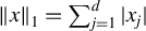 $\left \lVert x\right \rVert _1 = \sum _{j = 1}^d|x_j|$
,
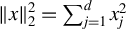 $\left \lVert x\right \rVert _2^2 = \sum _{j = 1}^d x_j^2$
, and
 $\left \lVert x\right \rVert _\infty = \max _{1\leq j \leq d}|x_j|$
.
3 LINEAR MODEL STABILITY ASSUMING BOUNDED SECOND MOMENTS
In this section, we assume that the returns process
 $V_t = (Y_t, X_t) \in \mathbb {R}\times \mathbb {R}^d$
is a Lévy process whose increments have a finite second moment,
 $\mathbb {E}\left \lVert V_{\Delta t}\right \rVert _2^2 < \infty $
, and that the least-squares estimator
 $\theta ^*$
is well-defined. The main assumptions are stated explicitly then followed by interpretations. The main result is provided next with a number of corollaries summarizing special cases. From an application point of view, these results reflect a single risky asset driven by a set of d factors.
In the second part of this section, we consider
 $V_t = (Y_t, X_t) \in \mathbb {R}^m\times \mathbb {R}^d$
which concerns m risky assets driven by a set of d common factors. In this setup, we consider how the rate of convergence results may change for portfolios constructed from the basic risky assets. From an econometric viewpoint, this analysis covers the combination of cross-sectional and temporal aggregation.
3.1 Aggregation across Time
Before we begin with the formal discussion, we show that linear conditional means have a simple stability property. In essence, if a Lévy process has an increment with a linear conditional mean then the conditional mean of any other increment is linear as well. This property does not require bounded second moments. It suffices to assume existence of the mean only.
Theorem 1. Suppose that
 $V_t = (Y_t, X_t)$
is a zero-mean Lévy process. If for some
 $t = \tau ,$
the conditional mean
 $\mathbb {E}(Y_{\tau } | X_{\tau })$
is linear with a vector of parameters
 $\theta $
, then the conditional mean
 $\mathbb {E}(Y_{t} | X_{t})$
is linear with the same vector of parameters for any
 $t \geq 0$
.
In the remaining part of this section, we show that, under certain assumptions, the conditional mean
 $\mathbb {E}(Y_{t} | X_{t})$
of the process
 $V_t$
becomes asymptotically linear if
 $t/\tau $
is sufficiently large regardless of the functional form of
 $\mathbb {E}(Y_{\tau } | X_{\tau })$
and we estimate the rate of convergence. The main assumptions are listed below.
Assumption 1. The random vector
 $V_{\Delta t} = (Y_{\Delta t}, X_{\Delta t}) \in \mathbb {R}\times \mathbb {R}^d$
is an increment of a Lévy process with
 $\mathbb {E}(V_{\Delta t}) = 0$
and
 $\mathbb {E}\left \lVert V_{\Delta t}\right \rVert _2^2 < \infty $
. The matrix
 $\mathbb {E}[X_{\Delta t}X_{\Delta t}^{\mathsf {T}}]$
is assumed invertible.
Assumption 2. The following moment conditions hold:
 $$ \begin{align} \mathbb{E}\left((Y_{\Delta t} - X_{\Delta t}^{\mathsf{T}} \theta^*)X^{\nu}_{\Delta t}\right) &= 0, \quad \forall \nu\colon |\nu| \leq k \end{align} $$
 $$ \begin{align} \mathbb{E}\left(|Y_{\Delta t} - X_{\Delta t}^{\mathsf{T}}\theta^*|\left\lVert X_{\Delta t}\right\rVert_1^{r}\right) &< \infty, \end{align} $$
where
 $k \geq 1$
is an integer,
 $\theta ^*$
is provided in equation (4),
 $\nu $
denotes a multi-index, and
 $r = k + \delta $
with
 $\delta \in (0, 1]$
.
The role of the assumptions can be explained in the following way. Assumption 1 defines the process and guarantees existence of
 $\theta ^*$
while Assumption 2 ensures boundedness of the functional
 $\boldsymbol {b}_r$
defined in equation (8).Footnote
5
Concerning the moment conditions in equation (11), note that
 $V_{\Delta t}$
is assumed to have a mean of zero in Assumption 1, which guarantees equation (11) holds for
 $k = 0$
. From the definition of
 $\theta ^*$
in equation (4), it follows directly that
 $\mathbb {E}[(Y_{\Delta t} - X_{\Delta t}^{\mathsf {T}}\theta ^*)X_{\Delta t}] = 0$
and, therefore, equation (11) holds automatically for
 $k = 1$
as well. Thus, the moment conditions are needed only for
 $k \geq 2$
.
The condition in equation (12) looks complicated but a simpler upper bound is easy to obtain. Indeed, the next inequality holds
 $$ \begin{align} \mathbb{E}\left(|Y_{\Delta t} - X_{\Delta t}^{\mathsf{T}}\theta^*|\left\lVert X_{\Delta t}\right\rVert_1^{r}\right) \leq \max(1, \left\lVert\theta^*\right\rVert_{\infty})\mathbb{E}\left\lVert V_{\Delta t}\right\rVert_1^{r+1}. \end{align} $$
An advantage is that we can isolate a simple moment condition involving the vector
 $V_{\Delta t}$
separately from
 $\theta ^*$
.
The main result is provided in the following theorem.
Theorem 2. Under Assumptions 1 and 2,
 $$ \begin{align} \boldsymbol{\varsigma}(n^{-1/2}V_{n\Delta t}) \leq C_{r}n^{1-\frac{r + 1}{2}}\boldsymbol{b}_{r}(V_{\Delta t}), \end{align} $$
where
 $r \geq 1$
,
 $C_r = \sup _u\left \lVert u\right \rVert _1^r\psi (u)$
. Finally,
 $\boldsymbol {b}_{r}(V_{\Delta t})$
can be bounded in the following way:
 $$ \begin{align} \boldsymbol{b}_{r}(V_{\Delta t}) \leq A_\delta \frac{\Gamma(\delta + 1)}{\Gamma(r + 1)}\mathbb{E}\left(|Y_{\Delta t} - X_{\Delta t}^{\mathsf{T}}\theta^*|\left\lVert X_{\Delta t}\right\rVert_1^{r}\right), \end{align} $$
in which
 $r = k + \delta $
,
 $k \geq 1$
is an integer, and
 $\delta \in (0, 1]$
,
 $A_{\delta } = \sup _{y \in \mathbb {R}}|y|^{-\delta }|e^{iy} - 1|$
is an absolute constant, and
 $\Gamma (x) = \int _0^\infty u^{x-1}e^{-u}du$
,
 $\operatorname {Re}(x)> 0$
, denotes the gamma function.
The constant
 $C_r$
depends entirely on the choice of the function
 $\psi $
and can be computed explicitly in some instances. For example, we prove in Lemma A.4 that if
 $\psi $
is chosen to be the ch.f. of a d-dimensional Gaussian distribution with standardized independent components,
 $\psi (u) = \exp (-u^{\mathsf {T}} u/2)$
, then
 $C_r = e^{-\frac {r}{2}}(rd)^{\frac {r}{2}}$
. It is important to emphasize that the rate of convergence does not depend on the choice of
 $\psi $
.
Next, we consider an important special case. If we set
 $r = 1 + \delta $
with
 $\delta \in (0, 1]$
, then, as explained previously, the moment conditions in equation (11) are satisfied automatically. We obtain the following corollary.
Corollary 1. If Assumption 1 holds together with the moment condition in equation (12) with
 $r = 1 + \delta $
,
 $\delta \in (0, 1]$
, then
 $$ \begin{align*} \boldsymbol{\varsigma}(n^{-1/2} V_{n\Delta t}) &\leq n^{-\delta/2}C_{1+\delta}\boldsymbol{b}_{1+\delta}(V_{\Delta t}). \end{align*} $$
The corollary illustrates that the conditions in Assumption 2 determine the rate of decay in Theorem 2. Clearly, the rate of decay increases with r. At the limit, if
 $\mathbb {E}\left \lVert V_{\Delta t}\right \rVert ^{r} < \infty $
for all r, then, by (13), the condition in equation (12) holds for all r. In addition, if the conditions in equation (11) hold for all k, then for any analytic function
 $h\colon \mathbb {R}^d \rightarrow \mathbb {C,}$
we have
 $$ \begin{align*} \mathbb{E}[(Y_{\Delta t} - X_{\Delta t}^{\mathsf{T}}\theta^*)h(X_{\Delta t})] &= \mathbb{E}\left[(Y_{\Delta t} - X_{\Delta t}^{\mathsf{T}}\theta^*)\sum_{|\nu| = 0}^{\infty}\frac{\partial^\nu h(0)}{\nu!}X_{\Delta t}^{\nu}\right]\\ &= \sum_{|\nu| = 0}^{\infty}\frac{\partial^\nu h(0)}{\nu!}\mathbb{E}\left[(Y_{\Delta t} - X_{\Delta t}^{\mathsf{T}}\theta^*)X_{\Delta t}^{\nu}\right] \\ &= 0. \end{align*} $$
The family of functions
 $\{h_u(x) = e^{iu^{\mathsf {T}} x}, u\in \mathbb {R}^d\}$
belongs to that class and, therefore,
 $\mathbb {E}[(Y_{\Delta t} - X_{\Delta t}^{\mathsf {T}}\theta ^*)h_u(X_{\Delta t})] = \mathbb {E}[(Y_{\Delta t} - X_{\Delta t}^{\mathsf {T}}\theta ^*)e^{iu^{\mathsf {T}} X_{\Delta t}}] = 0$
for all
 $u\in \mathbb {R}^d$
, which means that
 $\mathbb {E}[Y_{\Delta t}|X_{\Delta t}] = X_{\Delta t}^{\mathsf {T}}\theta ^*$
almost surely. By Lemma A.5,
 $\boldsymbol {b}_r(V_{n\Delta t}) = 0$
and the upper bound in equation (14) equals zero for any n.
The moment conditions in equation (11) permit an econometric interpretation. It is straightforward to notice that they represent first-order conditions of a least-squares problem. Consider, for example, the case
 $k = 2$
. If we add the components of
 $X_{\Delta t}$
raised to the second power and all mixed products linearly, we obtain the following least-squares problem:
 $$\begin{align*}(\tilde{\theta}, \tilde{\beta}) = \arg\min_{(\theta, \beta)} \mathbb{E}\left(Y_{\Delta t} - X_{\Delta t}^{\mathsf{T}}\theta - \sum_{|\nu|=2}X_{\Delta t}^{\nu}\beta_{\nu}\right)^2, \end{align*}$$
where
 $\beta $
is a vector containing all the
 $\beta _\nu $
parameters. If the optimal solution is
 $(\tilde {\theta }, \tilde {\beta }) = (\theta ^*, 0)$
, then the moment conditions in equation (11) hold with
 $k = 2$
. Clearly,
 $\tilde {\beta } = 0$
does not necessarily imply a linear conditional mean but according to Theorem 2 it does imply a faster rate of convergence if the corresponding condition in equation (12) holds as well. The same analysis can be repeated when
 $k> 2$
.
The rate of decay in Theorem 2 is also affected by the choice of
 $\delta $
. The conditions in equations (12) and (13) indicate that
 $\delta $
is determined by the tail behavior of
 $V_{\Delta t}$
. For instance, suppose that the conditions in equation (11) hold for some fixed value of k and
 $\mathbb {E}\|V_{\Delta t}\|_{1}^{k + \delta + 1} < \infty $
for all
 $0 < \delta < \delta ^* \leq 1$
but
 $\mathbb {E}\|V_{\Delta t}\|_{1}^{k + \delta ^* + 1}$
is unbounded. This is possible for distributions with a Pareto-type tail, see Section 5.1.2 for an example. In this case,
 $\delta $
can be chosen to be close but below
 $\delta ^*$
bearing in mind a potential trade-off—as
 $\delta $
approaches
 $\delta ^*$
the rate of decay improves but the value of the scaling constant
 $\boldsymbol {b}_r(V_{\Delta t})$
may deteriorate. If the moment
 $\mathbb {E}\|V_{\Delta t}\|_{1}^{k + 2}$
exists, then we can set
 $\delta = 1$
. For example, if
 $\mathbb {E}\|V_{\Delta t}\|_{1}^{3} < \infty ,$
then Corollary 1 holds with
 $\delta = 1$
.
Another special case can be constructed by imposing additional properties on the random vector
 $V_{\Delta t}$
. Suppose that
 $V_{\Delta t}$
is symmetric,
 $V_{\Delta t} \overset {\scriptscriptstyle d}{=} -V_{\Delta t}$
. It is easy to see that the conditions in equation (11) hold for any even value of
 $|\nu |$
. As a result, the conditional mean converges to a linear function faster for symmetric distributions.
Corollary 2. If
 $V_{\Delta t} \overset {\scriptscriptstyle d}{=} -V_{\Delta t}$
and Assumption 1 holds together with the moment condition in equation (12) with
 $r = 2 + \delta $
,
 $\delta \in (0, 1]$
, then
 $$\begin{align*}\boldsymbol{\varsigma}(n^{-1/2} V_{n\Delta t}) \leq n^{-\frac{1 + \delta}{2}}C_{2+\delta}\boldsymbol{b}_{2+\delta}(V_{\Delta t}). \end{align*}$$
Modern CLT rate-of-convergence results for metrics with uniform structure include moment conditions similar to the ones in Assumption 2, see, for example, Rachev et al. (Reference Rachev, Klebanov, Stoyanov and Fabozzi2013, Thms 15.4.2 and 15.4.3 and Remark 15.4.4) and Section 4.1 for a more detailed discussion. In terms of our notation, these moment conditions take the following form:
 $$ \begin{align} \mathbb{E}(V_{\Delta t}^\gamma - Z^\gamma) &= 0,\quad \forall \gamma\colon |\gamma| \leq k \end{align} $$
 $$ \begin{align} {\boldsymbol{v}}_{r+1}(V_{\Delta t}, Z) &= \int_{\mathbb{R}^{d+1}}\left\lVert\xi\right\rVert_1^{r+1}|F - \Phi|(d\xi) < \infty, \end{align} $$
where
 $r = k + \delta $
,
 $\delta \in (0, 1]$
,
 $\gamma $
is a multi-index, Z denotes a
 $(d+1)$
-dimensional Gaussian vector, and F and
 $\Phi $
denote the distribution functions of
 $V_{\Delta t}$
and Z, respectively. The functional
 ${\boldsymbol {v}}_{s}$
is known as an absolute pseudomoment of order s and its role is illustrated in Section 4.1. Even though the left side of equation (11) for any fixed
 $\nu $
is a linear combination of some of the moments
 $\mathbb {E} [V_{\Delta t}^{\nu + 1}]$
, one key difference from equation (16) is that the conditions in Assumption 2 do not involve moments of the marginals of
 $V_{\Delta t}$
on a stand-alone basis. For this reason, the conditions in Assumption 2 are weaker than those in equation (16) and the rate of decay in Theorem 2 can be faster than the corresponding rate of convergence in the CLT implied by the conditions in equations (16) and (17).
A somewhat trivial illustration of this observation can be constructed in the following way. If we choose any multivariate law for
 $V_{\Delta t}$
with linear conditional expectations, then, by Theorem 1 and Lemma A.1, we have
 $\boldsymbol {\varsigma }(V_{n\Delta t}) = 0$
for all
 $n\geq 1$
regardless of the marginal distributions of
 $V_{\Delta t}$
. At the same time, the conditions in equation (16) may not hold for any
 $k \geq 3$
and the rate of convergence in the CLT for the chosen multivariate law may be as slow as the classical rate of
 $n^{-1/2}$
. Section 5.2 provides a non-trivial numerical example of this phenomenon.
3.2 Cross-Sectional Aggregation Combined with Temporal Aggregation
The simulation study by Granger and Lee (Reference Granger and Lee1999) concludes that if there are prominent factors with a nonlinear impact at micro-level, the nonlinear effects may persist in cross-sectionally aggregated data. In some applications, however, the aggregation process is applied jointly cross-sectionally and in the time dimension. In this section, we focus on the joint impact.
In finance, for example, portfolios are formed from individual stocks and portfolio returns can be viewed as cross-sectional weighted averages of stock returns while return frequency reflects temporal aggregation. In fact, factor models are commonly applied to portfolios rather than individual basic risky assets. In this section, we change the setting to accommodate linear combinations of Y variables interpreted as portfolios. We demonstrate that under fairly general conditions linear models can become more adequate for portfolios faster with n than for individual stocks when the data are temporally aggregated.
Consider a multivariate process
 $V_t = (Y_t, X_t) \in \mathbb {R}^m\times \mathbb {R}^d$
, where m denotes the number of basic risky assets and d denotes the number of factors. The linear combination
 $Y_{p,t} = \sum _{i = 1}^mw_iY_{i,t}$
denotes a portfolio of the basic risky assets, where
 $w_i \geq 0$
stand for portfolio weights. Even though we focus on long-only portfolios, a similar analysis holds in the general case. Finally, denote by
 ${\mathbf {T}}_jV_t = (Y_{j,t}, X_t)$
an operator that selects the j-th component of
 $Y_t$
together with all factors and let
 ${\mathbf {T}}_pV_t = (Y_{p,t}, X_t)$
be an operator that constructs the portfolio and selects all factors.
The two assumptions can be adapted in the following way. Assumption 1 holds for the whole vector
 $V_t$
while Assumption 2 is modified to hold only for a specific portfolio.
Assumption 2*. The following moment conditions hold for
 ${\mathbf {T}}_pV_{\Delta t} = (Y_{p,\Delta t}, X_{\Delta t})$
:
 $$ \begin{align} \mathbb{E}\left((Y_{p,\Delta t} - X_{\Delta t}^{\mathsf{T}} \theta^*_p)X^{\nu}_{\Delta t}\right) &= 0, \quad \forall \nu\colon |\nu| \leq k_p \end{align} $$
 $$ \begin{align} \mathbb{E}\left(|Y_{p,\Delta t} - X_{\Delta t}^{\mathsf{T}}\theta^*_p|\left\lVert X_{\Delta t}\right\rVert_1^{r_p}\right) &< \infty, \end{align} $$
where
 $Y_{p,t} = \sum _{i = 1}^mw_iY_{i,t}$
,
 $k_p \geq 1$
is an integer,
 $\nu $
denotes a multi-index,
 $r_p = k_p + \delta $
with
 $\delta \in (0, 1]$
, and
 $\theta ^*_p$
is provided by
 $$ \begin{align*} \theta^*_p = (\mathbb{E}[X_{\Delta t}X_{\Delta t}^{\mathsf{T}}])^{-1}\mathbb{E}[Y_{p,\Delta t}X_{\Delta t}]. \end{align*} $$
The next corollary follows directly from Theorem 2.
Corollary 3. Under Assumptions 1 and 2*,
 $$ \begin{align} \boldsymbol{\varsigma}(n^{-1/2}{\mathbf{T}}_pV_{n\Delta t}) \leq C_{r_p}n^{1-\frac{r_p + 1}{2}}\boldsymbol{b}_{r_p}({\mathbf{T}}_pV_{\Delta t}), \end{align} $$
where
 $r_p \geq 1$
.
Cross-sectional aggregation can improve the upper bound in (20) relative to the upper bounds of the individual assets when Corollary 3 is applied independently to
 ${\mathbf {T}}_jV_t$
. For example, let us assume the worst-case scenario. If
 $\mathbb {E}\left \lVert V_{\Delta t}\right \rVert _1^{2+\delta } < \infty $
, then (19) holds for any portfolio and any individual risky asset, respectively. As illustrated previously, the condition in (18) holds automatically for
 $k_p = 1$
for any portfolio as well. Therefore, the inequality in (20) takes the form
 $$ \begin{align*} \boldsymbol{\varsigma}(n^{-1/2}{\mathbf{T}}_pV_{n\Delta t}) &\leq C_{1+\delta}n^{-\frac{\delta}{2}}\boldsymbol{b}_{1+\delta}({\mathbf{T}}_pV_{\Delta t})\\ &\leq C_{1+\delta}n^{-\frac{\delta}{2}}\sum_{j = 1}^mw_j\boldsymbol{b}_{1+\delta}({\mathbf{T}}_jV_{\Delta t}), \end{align*} $$
where the second inequality follows easily from
 $\theta _p = \sum _{i = 1}^mw_i\theta _i^*$
and the definition of
 $\boldsymbol {b}_r$
. Even though in this case the rate of convergence is the same regardless of the weights, the corresponding upper bound for the portfolio is smaller than the average of the individual risky assets’ upper bounds.
Next, suppose
 $\mathbb {E}\left \lVert V_{\Delta t}\right \rVert _1^{3+\delta } < \infty $
. Also, assume the condition in equation (18) does not hold for
 $\nu \colon |\nu |> 1$
for any of the individual assets. The condition in (18) for any portfolio can be expressed through the weights and the individual assets in the following way:
 $$ \begin{align*} \mathbb{E}\left((Y_{p,\Delta t} - X_{\Delta t}^{\mathsf{T}} \theta^*_p)X^{\nu}_{\Delta t}\right) &= \mathbb{E}\left[\left(\sum_{j = 1}^mw_jY_{j,\Delta t} - X_{\Delta t}^{\mathsf{T}} \left(\sum_{j = 1}^mw_j\theta^*_j\right)\right)X^{\nu}_{\Delta t}\right]\\ &= \sum_{j = 1}^mw_j\mathbb{E}\left((Y_{j,\Delta t} - X_{\Delta t}^{\mathsf{T}} \theta^*_j)X^{\nu}_{\Delta t}\right). \end{align*} $$
Thus, the condition in (18) for
 $k_p = 2$
can be written as
 $$ \begin{align} \sum_{j = 1}^mw_j\mathbb{E}\left((Y_{j,\Delta t} - X_{\Delta t}^{\mathsf{T}} \theta^*_j)X^{\nu}_{\Delta t}\right) = 0,\qquad \forall \nu\colon |\nu| = 2, \end{align} $$
because it holds for
 $\nu \colon |\nu | = 1$
by assumption. The number of equations in (21) equals
 $d + d(d-1)/2$
and this number depends only on the dimension d of the vector X. All of the equations are linear with respect to the portfolio weights. Therefore, if
 $$ \begin{align} d + \frac{d(d - 1)}{2}< m, \end{align} $$
then there exists a portfolio (possibly a long-short one) for which (21) holds. As a consequence, for that portfolio
 $r_p = 2+\delta $
and the inequality in (20) becomes
 $$\begin{align*}\boldsymbol{\varsigma}(n^{-1/2}{\mathbf{T}}_pV_{n\Delta t}) \leq C_{2+\delta}n^{-\frac{\delta + 1}{2}}\boldsymbol{b}_{2+\delta}({\mathbf{T}}_pV_{\Delta t}). \end{align*}$$
As a result, the rate of decay
 $(\delta + 1)/2$
is strictly faster than the rate
 $\delta /2$
of the individual risky assets. Section 5.1.3 includes a simple illustration with the hyperbolic skewed-t distribution.
In the practice of finance, factor models are usually of low dimension while the cross section, depending on which universe is considered, typically contains a large number of stocks. Thus, the left side of the inequality in equation (22) is in practice much smaller than m. For example,
 $m = 1,000$
for the large cap Russell 1,000 universe, while for a ten-factor model, the left side equals 55.Footnote
6
In the academic literature, very popular factor models include the three-factor model of Fama and French (Reference Fama and French1992), the four-factor model of Carhart (Reference Carhart1997), and the five-factor model of Fama and French (Reference Fama and French2015). Even though there is a debate about the dimension of the factor space, it is generally believed to be low (Feng et al., Reference Feng, Giglio and Xiu2020).
4 THE CASE OF INFINITE VARIANCE
Dropping the assumption of finite second moment for the process
 $\{V_t, t> 0\}$
leads to a number of difficulties with the approach developed in Section 3. First, the normalization by
 $n^{-1/2}$
is no longer correct and, second, the least-squares solution in equation (4) is irrelevant as it involves diverging quantities. Finally and perhaps most importantly, all moments involved in the conditions in Assumption 2 are unbounded. As a result, the functional
 $\boldsymbol {b}_r(V_{\Delta t})$
is unbounded as well for any
 $r \geq 1$
and the upper bound in Theorem 2 becomes impractical.
These observations indicate that the infinite variance case requires a different treatment. We adopt a strategy similar to that behind the rate-of-convergence theorems for the GCLT. In essence, we need new assumptions involving moment conditions defined on the difference of
 $V_t$
and another process which appears as the corresponding limit under the GCLT. In this section, we take advantage of this approach and we generalize Theorem 2.
Denote by
 $Z_t = (Z_{y,t}, Z_{x,t}) \in \mathbb {R}\times \mathbb {R}^d$
a strictly
 $\alpha $
-stable Lévy process independent of
 $V_t$
. The ch.f. of the increment
 $Z_1 - Z_0 = Z_1$
takes the form (Sato, Reference Sato1999, Thm. 14.10)
 $$ \begin{align} \varphi(u) = \exp\left\{-\int_{\mathbb{S}}|u^{\mathsf{T}}\xi|^\alpha\left(1 - i\,\mathrm{sign}(u^{\mathsf{T}}\xi)\tan\frac{\pi\alpha}{2}\right)\Lambda_1(d\xi)\right\}, \end{align} $$
where
 $\alpha \in (0, 2]$
is the tail parameter,
 $\mathbb {S} = \{z\in \mathbb {R}\times \mathbb {R}^d\colon \|z\|_2 = 1\}$
denotes the unit sphere in
 $\mathbb {R}^{d+1}$
, and
 $\Lambda _1$
denotes a finite nonzero measure defined on the Borel subsets of
 $\mathbb {S}$
, also known as the spectral measure. We assume that
 $\mathbb {E}|Z_1| < \infty $
which implies that
 $1 < \alpha \leq 2$
. Finally, strict stability in this case means
 $\mathbb {E}(Z_1) = 0$
.
In the finite-variance case, the vector of parameters
 $\theta $
is determined by the least-squares solution. In the infinite variance case, if
 $V_{\Delta t}$
is in the domain of attraction of a stable law whose corresponding conditional mean is linear, then, by Theorem 1, the vector
 $\theta $
is determined by the spectral measure
 $\Lambda _1$
. In Lemma A.6, we prove that if
 $\theta _\alpha ^{*}$
solves
 $$ \begin{align} &\int_{\mathbb{S}}(y - x^{\mathsf{T}}\theta_\alpha^{*})\,\mathrm{sign}(u^{\mathsf{T}} x)|u^{\mathsf{T}} x|^{\alpha - 1}\Lambda_1 (d\xi) = 0,\quad \forall u \in \mathbb{R}^d \end{align} $$
 $$ \begin{align} &\int_{\mathbb{S}}(y - x^{\mathsf{T}}\theta_\alpha^{*})|u^{\mathsf{T}} x|^{\alpha - 1}\Lambda_1(d\xi) = 0,\quad \forall u \in \mathbb{R}^d, \end{align} $$
where
 $\xi = (y,x)$
, then
 $\mathbb {E}(Z_{y,1}|Z_{x,1}) = Z_{x,1}^{\mathsf {T}}\theta _\alpha ^*$
almost surely and vice versa. By Theorem 1, if
 $\theta _\alpha ^{*}$
solves the equations above, then
 $\mathbb {E}(Z_{y,t}|Z_{x,t}) = Z_{x,t}^{\mathsf {T}}\theta _\alpha ^*$
almost surely for any t.
These conditions appear complicated and the following special cases provide some clarification. If
 $Z_1$
is symmetric, then
 $\Lambda _1$
is symmetric and the condition in equation (25) is satisfied automatically. The necessary and sufficient condition in equation (24) for the symmetric case is derived in Miller (Reference Miller1978). Even in the symmetric case,
 $\theta _\alpha ^{*}$
may not be determined uniquely, which is a clear difference from the finite-variance case. If
 $\alpha = 2$
, then
 $Z_1$
follows a Gaussian distribution and we are in the finite-variance case. In this situation, equation (24) reduces to the least-squares case, that is,
 $\theta _2^* = \theta ^*$
.
We replace Assumptions 1 and 2 with the following ones.
Assumption 1†. The random vector
 $V_{\Delta t} = (Y_{\Delta t}, X_{\Delta t}) \in \mathbb {R}\times \mathbb {R}^d$
is an increment of a Lévy process with
 $\mathbb {E}(V_{\Delta t}) = 0$
. The random vector
 $Z_{\Delta t} = (Z_{y,\Delta t}, Z_{x,\Delta t}) \in \mathbb {R}\times \mathbb {R}^d$
is an increment of a strictly
 $\alpha $
-stable process with
 $\alpha \in (1, 2]$
and there exists a vector of parameters
 $\theta _\alpha ^*$
satisfying equations (24) and (25).
Assumption 2†. The following moment conditions hold:
 $$ \begin{align} \int_{\mathbb{R}^{d+1}}(y - x^{\mathsf{T}}\theta^*_\alpha)x^\nu d(F - G) &= 0, \quad \forall \nu\colon |\nu| \leq k \end{align} $$
 $$ \begin{align} \int_{\mathbb{R}^{d+1}}|y - x^{\mathsf{T}}\theta^*_\alpha|\left\lVert x\right\rVert_1^r|F - G|(d\xi) &< \infty, \end{align} $$
where
 $\xi = (y,x) \in \mathbb {R}\times \mathbb {R}^d$
, F is the distribution function of
 $V_{\Delta t}$
, G is the distribution function of
 $Z_{\Delta t}$
,
 $k \geq 1$
is an integer,
 $\theta ^*_\alpha $
satisfies equations (24) and (25),
 $\nu $
denotes a multi-index, and
 $r = k + \delta $
with
 $\delta \in (0, 1]$
.
Finally, we need a version of
 $\boldsymbol {b}_r(V_{t})$
defined in equation (8), which is well behaved in the infinite variance case. Consider
 $$ \begin{align} \boldsymbol{b}_r^\theta(V_t, Z_t) = \sup_u\left\lVert u\right\rVert_1^{-r}\left|\int_{\mathbb{R}^{d+1}}(y - x^{\mathsf{T}}\theta)e^{i u^{\mathsf{T}} x}d(F_{V_t}-G_{Z_t}) \right|, \end{align} $$
where
 $F_{V_t}$
and
 $G_{Z_t}$
are the distribution functions of
 $V_t$
and
 $G_t$
, respectively. The important difference from
 $\boldsymbol {b}_r(V_{t})$
is that the limit law is subtracted, which regularizes the behavior of the integral at
 $u = 0$
. Lemma A.8 shows that if the conditions in Assumption 2†
are satisfied for some
 $\theta $
and arbitrary
 $V_{\Delta t}$
and
 $Z_{\Delta t}$
, then
 $\boldsymbol {b}_r^\theta (V_{\Delta t}, Z_{\Delta t}) < \infty $
.
Similarly to the finite-variance case, we can find a simpler bound for equation (27). The same approach leads to
 $$ \begin{align} \int_{\mathbb{R}^{d+1}}|y - x^{\mathsf{T}}\theta^*_\alpha|\left\lVert x\right\rVert_1^r|F - G|(d\xi) &\leq K\int_{\mathbb{R}^{d+1}}\left\lVert\xi\right\rVert_1^{r+1}|F - G|(d\xi)\\ &= K{\boldsymbol{v}}_{r+1}(V_{\Delta t}, Z_{\Delta t}),\nonumber \end{align} $$
where
 $K = \max (1, \left \lVert \theta ^*_\alpha \right \rVert _{\infty })$
. The inequality in (29) can be combined with Lemma A.8 to conclude that existence of the absolute pseudomoment of order
 $r+1$
between the increments
 $V_{\Delta t}$
and
 $Z_{\Delta t}$
, together with the conditions in (26), guarantees boundedness of
 $\boldsymbol {b}_r^\theta (V_{\Delta t}, Z_{\Delta t})$
.
A generalization of Theorem 2 is provided below.
Theorem 3. Under Assumptions 1† and 2† ,
 $$ \begin{align} \boldsymbol{\varsigma}\left(n^{-1/\alpha}V_{n\Delta t}\right) \leq C_r n^{1 - \frac{r+1}{\alpha}}\boldsymbol{b}_r^{\theta^*_\alpha}(V_{\Delta t}, Z_{\Delta t}), \end{align} $$
where
 $r = k + \delta $
,
 $k \geq 1$
is an integer,
 $\delta \in (0, 1]$
, and
 $C_r = \sup _u\left \lVert u\right \rVert _1^r\psi (u)$
. Finally, the next bound holds
 $$\begin{align*}\boldsymbol{b}_r^{\theta^*_\alpha}(V_{\Delta t}, Z_{\Delta t}) \leq A_\delta\frac{\Gamma(\delta + 1)}{\Gamma(r + 1)}\int_{\mathbb{R}^{d+1}}|y - x^{\mathsf{T}}\theta^*_\alpha|\left\lVert x\right\rVert_1^r|F - G|(d\xi), \end{align*}$$
in which
 $\xi = (y,x)$
,
 $A_{\delta } = \sup _{y \in \mathbb {R}}|y|^{-\delta }|e^{iy} - 1|$
is an absolute constant, and
 $\Gamma (x)$
denotes the gamma function.
Theorem 2 arises as a special case when
 $\alpha = 2$
in the following way. First, as noted earlier, the distribution of
 $Z_{\Delta t}$
in this case is Gaussian and the ch.f. in (23) turns into the Gaussian ch.f. In fact,
 $\Lambda _1$
is no longer unique and there are many symmetric choices for
 $\Lambda _1$
converting the ch.f. in equation (23) into the Gaussian ch.f. (Samorodnitsky and Taqqu, Reference Samorodnitsky and Taqqu1994, Sect. 2.4). As a consequence, the condition in (25) is satisfied due to symmetry considerations and
 $\theta _2^* = {\mathbf {C}}_{xx}^{-1}{\mathbf {C}}_{yx}$
is the unique solution of (24), where
 ${\mathbf {C}}$
is the covariance matrix of
 $Z_{\Delta t}$
and the indices indicate the blocks corresponding to the y and x components of the vector
 $(Z_{y,\Delta t}, Z_{x,\Delta t})$
.
Second, the condition in equation (26) holds with
 $|\nu | = 1$
if
 $\mathbb {E}[Z_{\Delta t}] = 0$
. It holds with
 $|\nu | = 2$
only if
 ${\mathbf {C}}$
coincides with the covariance matrix of the vector
 $V_{\Delta t}$
. As a consequence,
 $\theta _2^* = \theta ^*$
, where
 $\theta ^*$
is provided in equation (4). Separately, the vector
 $Z_{\Delta t}$
has linear conditional means and, therefore,
 $\mathbb {E}[(Z_{y,\Delta t} - Z_{x,\Delta t}^{\mathsf {T}}\theta ^*)f(Z_{x,\Delta t})] = 0$
for any measurable function f for which the moment is defined. This shows that
 $\mathbb {E}[(Z_{y,\Delta t} - Z_{x,\Delta t}^{\mathsf {T}}\theta ^*)Z_{x,\Delta t}^\nu ] = 0$
,
 $\forall \nu \colon |\nu | \leq k$
and the condition in equation (26) turns into that in equation (11) after writing the integral as a difference of two expectations.
In a similar way, for the left side of (27), we obtain
 $$\begin{align*}|I_V - I_Z| \leq \int_{\mathbb{R}^{d+1}}|y - x^{\mathsf{T}}\theta^*_\alpha|\left\lVert x\right\rVert_1^r|F - \Phi|(d\xi) \leq I_V + I_Z, \end{align*}$$
where
 $I_V = \mathbb {E}(|Y_{\Delta t} - X_{\Delta t}^{\mathsf {T}}\theta ^*|\left \lVert X_{\Delta t}\right \rVert _1^{r})$
,
 $I_Z = \mathbb {E}(|Z_{y, \Delta t} - Z_{x, \Delta t}^{\mathsf {T}}\theta ^*|\left \lVert Z_{x, \Delta t}\right \rVert _1^{r})$
, and
 $\Phi $
denotes the distribution function of the increment
 $Z_{\Delta t}$
. As a consequence, the condition in equation (27) becomes effectively the same as that in equation (12) because the term
 $I_Z$
involving
 $Z_{\Delta t}$
is always bounded.
As a result of this analysis, Assumptions 1†
and 2†
become essentially the same as Assumptions 1 and 2 when
 $\alpha = 2$
. It remains to demonstrate how the functional in the upper bound in equation (30) reduces to the one in equation (14). Given that the distribution of
 $Z_{\Delta t}$
is Gaussian, the conditional means of
 $Z_{\Delta t}$
are linear and
 $\boldsymbol {b}_r(Z_{\Delta t}) = 0$
. Furthermore, from the conditions in Assumption 2, we conclude that
 $\boldsymbol {b}_r(V_{\Delta t})$
is bounded. Thus, we can represent the integral in the definition of
 $\boldsymbol {b}_r^{\theta ^*}(V_{\Delta t}, Z_{\Delta t})$
in equation (28) as a difference of two well-defined integrals
 $$ \begin{align} \begin{aligned} &\left\lVert u\right\rVert_1^{-r}\int_{R^{d+1}}(y - x^{\mathsf{T}}\theta^*)e^{i u^{\mathsf{T}} x}d(F-\Phi) \\ &\qquad\qquad =\left\lVert u\right\rVert_1^{-r}\int_{R^{d+1}}(y - x^{\mathsf{T}}\theta^*)e^{i u^{\mathsf{T}} x}dF - \left\lVert u\right\rVert_1^{-r}\int_{R^{d+1}}(y - x^{\mathsf{T}}\theta^*)e^{i u^{\mathsf{T}} x}d\Phi\\ &\qquad\qquad =\left\lVert u\right\rVert_1^{-r}\int_{R^{d+1}}(y - x^{\mathsf{T}}\theta^*)e^{i u^{\mathsf{T}} x}dF. \end{aligned} \end{align} $$
As a consequence,
 $$\begin{align*}\boldsymbol{b}_r^{\theta^*}(V_{\Delta t}, Z_{\Delta t}) = \boldsymbol{b}_r(V_{\Delta t}) \end{align*}$$
and the upper bound in Theorem 3 is indeed the same as the upper bound in Theorem 2.
Finally, we note that under Assumption 1†
, when
 $\alpha < 2,$
the calculation in (31) is not possible because the two quantities on the right side are not finite on a stand-alone basis even though the left side can be, as shown in Lemma A.8.
4.1 A Connection with the Generalized CLT
It is important to note that in the infinite variance case, the limit law may have nonlinear conditional means, see Samorodnitsky and Taqqu (Reference Samorodnitsky and Taqqu1994, Chap. 5) for a complete characterization of the bivariate case. Therefore, if no vector of parameters solves equations (24) and (25), then
 $\boldsymbol {\varsigma }(n^{-1/\alpha }V_{n\Delta t})$
does not decay. Next, we discuss this situation in more detail and we clarify a connection with a classical rate-of-convergence result in the GCLT setting. To simplify the expressions, we denote the expectation appearing in
 $\boldsymbol {\varsigma }(n^{-1/\alpha }V_{n\Delta t})$
and the corresponding expectation of the limit by
 $$ \begin{align*} \varpi_{\alpha, n}^\theta(u) &= \mathbb{E}\left[\frac{1}{n^{1/\alpha}}(Y_{n\Delta t} - X_{n\Delta t}^{\mathsf{T}}\theta)e^{iu^{\mathsf{T}} \frac{1}{n^{1/\alpha}}X_{n\Delta t}}\right]\\ \varpi_{\alpha}^\theta(u) &= \mathbb{E}(Z_{y,\Delta t} - Z_{x,\Delta t}^{\mathsf{T}}\theta)e^{iu^{\mathsf{T}} Z_{x,\Delta t}}, \end{align*} $$
where
 $\theta $
is the same in both expressions.
The result in this section involves the following weighted metric between the ch.f. of two random vectors U and W,
 $$ \begin{align} {\boldsymbol{\chi}}_s(U,W) = \sup_u\left\lVert u\right\rVert_1^{-s}|\mathbb{E} e^{iu^{\mathsf{T}} U} - \mathbb{E} e^{iu^{\mathsf{T}} W}|, \end{align} $$
where
 $s \geq 0$
. A classical result in the rate-of-convergence problem for GCLT restated in our notation shows that if the next moment conditions hold,
 $$ \begin{align} \int_{\mathbb{R}^{d+1}}z^\gamma d(F - G) = 0, \ \forall \gamma\colon |\gamma| \leq \ell \quad \mathrm{and}\quad {\boldsymbol{v}}_{s}(V_{\Delta t}, Z_{\Delta t})< \infty, \end{align} $$
where
 $s = \ell + \delta $
,
 $\ell \geq 1$
is an integer,
 $\delta \in (0, 1]$
, the absolute pseudomoment
 ${\boldsymbol {v}}_s$
is provided in equation (17),
 $Z_{\Delta t}$
has an
 $\alpha $
-stable distribution, and
 $\gamma $
is a multi-index, then
 $$ \begin{align} {\boldsymbol{\chi}}_s\left(n^{-1/\alpha}V_{n\Delta t},\,n^{-1/\alpha}Z_{n\Delta t}\right) \leq n^{1 - s/\alpha}{\boldsymbol{\chi}}_s(V_{\Delta t}, Z_{\Delta t}), \end{align} $$
in which
 $s> \alpha $
and the right side is finite (Rachev et al., Reference Rachev, Klebanov, Stoyanov and Fabozzi2013, Chap. 15). The metric
 ${\boldsymbol {\chi }}_s$
satisfies a set of properties which define it as an ideal probability metric of order s and the inequality in equation (34) is a direct consequence of them.Footnote
7
The conditions in equations (16) and (17) are the same as the ones in equation (33) when
 $Z_{\Delta t}$
has a multivariate Gaussian distribution and the upper bound in equation (34) holds for the CLT with
 $\alpha = 2$
.
The connection between the GCLT and Theorem 3 is provided below. Basically, the moment conditions in equation (33) replace Assumption 2†
and the limiting distribution is not assumed to have a linear conditional mean; that is, the part of Assumption 1†
involving the existence of
 $\theta _\alpha ^*$
is ignored.
Theorem 4. Suppose the random vector
 $V_{\Delta t} = (Y_{\Delta t}, X_{\Delta t}) \in \mathbb {R}\times \mathbb {R}^d$
is an increment of a Lévy process with
 $\mathbb {E}(V_{\Delta t}) = 0$
with distribution function F and
 $Z_{\Delta t} = (Z_{y,\Delta t}, Z_{x,\Delta t}) \in \mathbb {R}\times \mathbb {R}^d$
is an increment of a strictly
 $\alpha $
-stable process,
 $1 < \alpha \leq 2$
, with distribution function G. Also, suppose that the moment conditions in equation (33) hold with
 $s = k + \delta $
,
 $k \geq 2$
,
 $\delta \in (0, 1]$
. Then, the next inequality holds for any bounded
 $\theta $
,
 $$ \begin{align} \begin{aligned} \sup_u\left\{\psi(u)\left|\varpi_{\alpha, n}^\theta(u) - \varpi_{\alpha}^\theta(u)\right|\right\}&\leq C_{s-1}n^{1 - \frac{s}{\alpha}}\boldsymbol{b}_{s-1}^\theta(V_{\Delta t}, Z_{\Delta t}) \\ &\quad + \alpha C_{s - 1 +\alpha}D_\alpha n^{1 - \frac{s}{\alpha}}{\boldsymbol{\chi}}_s(X_{\Delta t}, Z_{x,\Delta t}), \end{aligned} \end{align} $$
where
 $\psi (u)> 0$
is the ch.f. of a symmetric random vector with a sufficiently smooth density,
 $C_p = \sup _u\left \lVert u\right \rVert _1^p\psi (u)$
,
 $D_\alpha = \sup _{t\in B}\left |\omega _{\alpha ,\Lambda }(t)\right |$
, in which
 $B = \{z\in \mathbb {R}^d\colon \left \lVert z\right \rVert _1=1\}$
and
 $\omega _{\alpha ,\Lambda }(t)$
is provided in Lemma A.9.
To illustrate the connection with Theorem 3, represent
 $z = (y, x_1, \ldots , x_d)$
and suppose that the conditions in equation (33) hold for some
 $\ell $
. Then, we have
 $$ \begin{align} \begin{aligned} \int_{\mathbb{R}^{d+1}}yx^\nu d(F - G) = 0\quad \text{and}\quad \int_{\mathbb{R}^{d+1}}x_jx^\nu d(F - G) = 0 \end{aligned} \end{align} $$
for all multi-indices
 $\nu \colon |\nu | = \ell -1$
and
 $j = 1,\ldots , d$
. It is easy to see that any linear combination of the integrals on the left side of (36) also vanishes and, therefore, the condition in equation (26) in Assumption 2†
holds for any choice of
 $\theta $
when
 $k = \ell - 1$
. Finally, the boundedness of the absolute pseudomoment
 ${\boldsymbol {v}}_s$
assumed in (33) combined with the inequality in (29) ensures that the moment condition in (27) in Assumption 2†
holds with
 $r = s - 1$
as well. As a consequence, Lemma A.8 shows that under these assumptions the functional
 $\boldsymbol {b}_r^\theta (V_{\Delta t}, Z_{\Delta t})$
exists for any bounded
 $\theta $
.Footnote
8
Since all quantities in the upper bound in (35) are finite, its right side provides a rate of convergence of
 $\varpi _{\alpha , n}^\theta $
to
 $\varpi _{\alpha }^\theta $
under the weighted uniform distance and, clearly,
 $\varpi _{\alpha }^\theta $
may not vanish for all values of u. However, if the corresponding conditional mean of the limit law is linear, then
 $\varpi _{\alpha }^{\theta }(u) = 0$
for all
 $u\in \mathbb {R}^d$
for some
 $\theta = \theta _\alpha ^*$
. In this situation, the constant
 $D_\alpha $
vanishes as well because in this case there exists
 $\theta _\alpha ^*$
satisfying equations (24) and (25) which, in turn, ensure
 $\omega _{\alpha ,\Lambda }(t) = 0$
for all
 $t \in \mathbb {R}^d$
.Footnote
9
As a result, the left side of (35) turns into
 $\boldsymbol {\varsigma }(n^{-1/\alpha }V_{n\Delta t})$
and the second term on the right side vanishes, which makes the right side of (35) the same as the upper bound in equation (30) in Theorem 3. Even though (30) can be viewed as a special case of equation (35), in practice, Theorem 3 is proved under weaker conditions.
5 NUMERICAL EXAMPLES AND FURTHER COMMENTS
This section includes numerical examples illustrating the behavior of the conditional mean of the normalized sum as a function of n, where we arbitrarily set
 ${\Delta t = 1}$
. Also, we provide additional comments concerning extensions of the theoretical setup. To simplify the notation further, we denote the properly normalized sum of increments by
 $$ \begin{align} \widetilde{V}_n = (\widetilde{Y}_n, \widetilde{X}_n) = \frac{1}{n^{1/\alpha}}\left(\sum_{k = 1}^n \Delta Y_k, \sum_{k = 1}^n \Delta X_k \right), \end{align} $$
where
 $\alpha \in (1, 2]$
.
The examples are constructed with flexible parametric classes illustrating both the finite and the infinite variance cases discussed in the article. It is convenient if the ch.f. of the increment enjoys a closed-form expression because of the next connection with the conditional mean (Samorodnitsky and Taqqu, Reference Samorodnitsky and Taqqu1994, Sect. 5.1). Suppose that the random vector
 $(Y, X) \in \mathbb {R}\times \mathbb {R}^d$
has a finite expectation and denote its ch.f. by
 $\phi (v,u) = \mathbb {E} e^{i(vY + u^{\mathsf {T}} X)}$
. The following expression holds:
 $$ \begin{align} \mathbb{E}[Y|X = x] = \frac{1}{2\pi f_{X}(x)}\int_{\mathbb{R}^d}\frac{\phi_v'(0,u)}{i}e^{-ix^{\mathsf{T}} u}du, \end{align} $$
where
 $\phi _v'(0,u) = \frac {\partial }{\partial v}\phi (v,u)|_{v = 0} = i\mathbb {E}(Ye^{iu^{\mathsf {T}} X})$
.
As a consequence, the conditional mean can be computed numerically with the fast Fourier transform (FFT) applied to the function
 $\frac {1}{i}\phi _v'(0,u)$
. In a similar vein, if the density
 $f_X(x)$
is not available in closed form, it can also be approximated with the FFT method applied to the marginal ch.f.
 $\phi _X(u) = \phi (0, u)$
.
5.1 Hyperbolic Skewed-t Examples
The hyperbolic skewed-t process is a special case of the generalized hyperbolic process which has received a lot of attention in the finance literature (Eberlein, Reference Eberlein, Barndorff-Nielsen, Mikosch and Resnick2001; McNeil, Frey, and Embrechts, Reference McNeil, Frey and Embrechts2005; Bianchi et al., Reference Bianchi, Stoyanov, Tassinari, Fabozzi and Focardi2019). Suppose that the vector
 $V_1 \in \mathbb {R}^{m + d}$
has a hyperbolic skewed-t distribution denoted by
 $V_1 \in \mathrm {HSt}_{\lambda }(\mu , \beta , \Sigma , \chi )$
and defined by the following ch.f.:
 $$ \begin{align*} \phi_1(z) = \frac{2^{1 + \lambda}e^{iz^{\mathsf{T}}\mu}}{\Gamma(-\lambda)}\left(-2\chi\left(iz^{\mathsf{T}}\beta - \frac{1}{2}z^{\mathsf{T}}\Sigma z\right)\right)^{-\lambda/2}K_\lambda\left(\sqrt{-2\chi\left(iz^{\mathsf{T}}\beta - \frac{1}{2}z^{\mathsf{T}}\Sigma z\right)}\right), \end{align*} $$
in which we set
 $z = (v, u) \in \mathbb {R}^{m + d}$
and
 $K_\lambda (x) = \frac {1}{2}\int _{0}^{\infty }t^{\lambda - 1}e^{-x(t+t^{-1})/2}dt$
,
 $x> 0, $
denotes the Bessel function of the second kind. The parameters have the following interpretations:
 $\mu \in \mathbb {R}^{m + d}$
is a location parameter,
 $\beta \in \mathbb {R}^{m + d}$
is a skewness parameter,
 $\Sigma $
is an
 $(m + d)\times (m + d)$
symmetric matrix,
 $\chi> 0$
acts like a scaling parameter, and
 $\lambda < 0$
is a shape parameter.
Most of the intuition behind the interpretation of the parameters follows from the normal location-scale mixture representation:
 $$ \begin{align} V_1 = \mu + \beta W + \sqrt{W}Z, \end{align} $$
where W has an inverse gamma distribution
 $\mathrm {IG}(-\lambda , \chi /2)$
and
 $Z \in \mathcal {N}(0, \Sigma )$
has a multivariate Gaussian distribution with covariance matrix
 $\Sigma $
. From this representation, it is easy to see that linear transformations belong to the same class. Suppose that
 $\mathbf {A}$
is a
 $q\times (m + d)$
matrix. Then,
 $\mathbf {A} V_1 \in \mathrm {HSt}_\lambda (\mathbf {A}\mu , \mathbf {A}\beta , \mathbf {A}\Sigma \mathbf {A}^{\mathsf {T}}, \chi )$
.
Following Section 3.2, partition the random vector
 $V_1$
in the following manner
 $V_1 = (Y_1, X_1) \in \mathbb {R}^m\times \mathbb {R}^d$
. The parameters of the distribution are partitioned accordingly
 $$ \begin{align*} \mu = \begin{pmatrix} \mu_Y \\ \mu_X \end{pmatrix},\qquad \beta = \begin{pmatrix} \beta_Y \\ \beta_X \end{pmatrix},\qquad \Sigma = \begin{pmatrix} \Sigma_{YY} & \Sigma_{YX} \\ \Sigma_{XY} & \Sigma_{XX} \end{pmatrix}. \end{align*} $$
Jamalizadeh and Balakrishnan (Reference Jamalizadeh and Balakrishnan2019) provide an expression for the conditional mean of a general normal location-scale mixture which takes the following form:
 $$ \begin{align} \mathbb{E}(Y_1 | X_1 = x) = \mu_Y + \Sigma_{YX}\Sigma_{XX}^{-1}(x - \mu_X) + (\beta_{Y} - \Sigma_{YX}\Sigma_{XX}^{-1}\beta_{X})\mathbb{E} W_x, \end{align} $$
where
 $W_x$
denotes the conditional distribution
 $W|(X_1 = x)$
. As a consequence, the conditional mean is linear if and only if
 $\beta _{Y} = \Sigma _{YX}\Sigma _{XX}^{-1}\beta _{X}$
. Even though the expectation
 $\mathbb {E} W_x$
can be computed explicitly for the hyperbolic skewed-t distribution, we do not work with these expressions because the class is not closed with respect to the convolution operation. However, the ch.f. of the normalized sum
 $\widetilde {V}_n$
is easy to write down and the conditional mean can be computed numerically using equation (38).
The hyperbolic skewed-t has both finite and infinite variance representatives. The tail behavior of the distribution can be summarized in the following way. If we take a linear combination
 $w^{\mathsf {T}} V_1$
with
 $w^{\mathsf {T}} \beta> 0$
, then the asymptotic decay of the density is given by
 $$ \begin{align*} f_{w^{\mathsf{T}} V_1}(y) &\sim |y|^{\lambda - 1}e^{-2w^{\mathsf{T}} \beta y},\qquad y\rightarrow\infty\\ f_{w^{\mathsf{T}} V_1}(y) &\sim |y|^{\lambda - 1},\qquad y\rightarrow -\infty. \end{align*} $$
As a consequence,
 $V_1$
has a finite expectation if
 $\lambda < -1$
and a finite variance if
 $\lambda < -2$
. The asymptotic property of the tail also suggests the correct exponent
 $\alpha $
in the normalization in (37) is
 $\alpha = \min (-\lambda , 2)$
.
5.1.1 Convergence to a Linear Function
Our first example is an illustration of the convergence result in Section 3. We assume
 $m = 1$
,
 $d = 1$
and that
 $V_1$
has a finite variance and a nonlinear conditional mean. In terms of parameters, we pick
 $\lambda = -5$
,
 $\chi = 1$
,
 $$\begin{align*}\beta = \begin{pmatrix} -2 \\ 2 \end{pmatrix},\qquad \mu = \frac{\chi}{2(\lambda + 1)}\beta, \qquad \text{and}\qquad \Sigma = \begin{pmatrix} 1 & 0.5 \\ 0.5 & 1 \end{pmatrix}. \end{align*}$$
The value for
 $\mu $
ensures that the distribution has a mean of zero, the remaining values are chosen for convenience. The shape of the conditional mean as function of the number of summands n is provided in Figure 1. The x-axis covers the range from the 1%-quantile to the 99%-quantile of the distribution of
 $X_1$
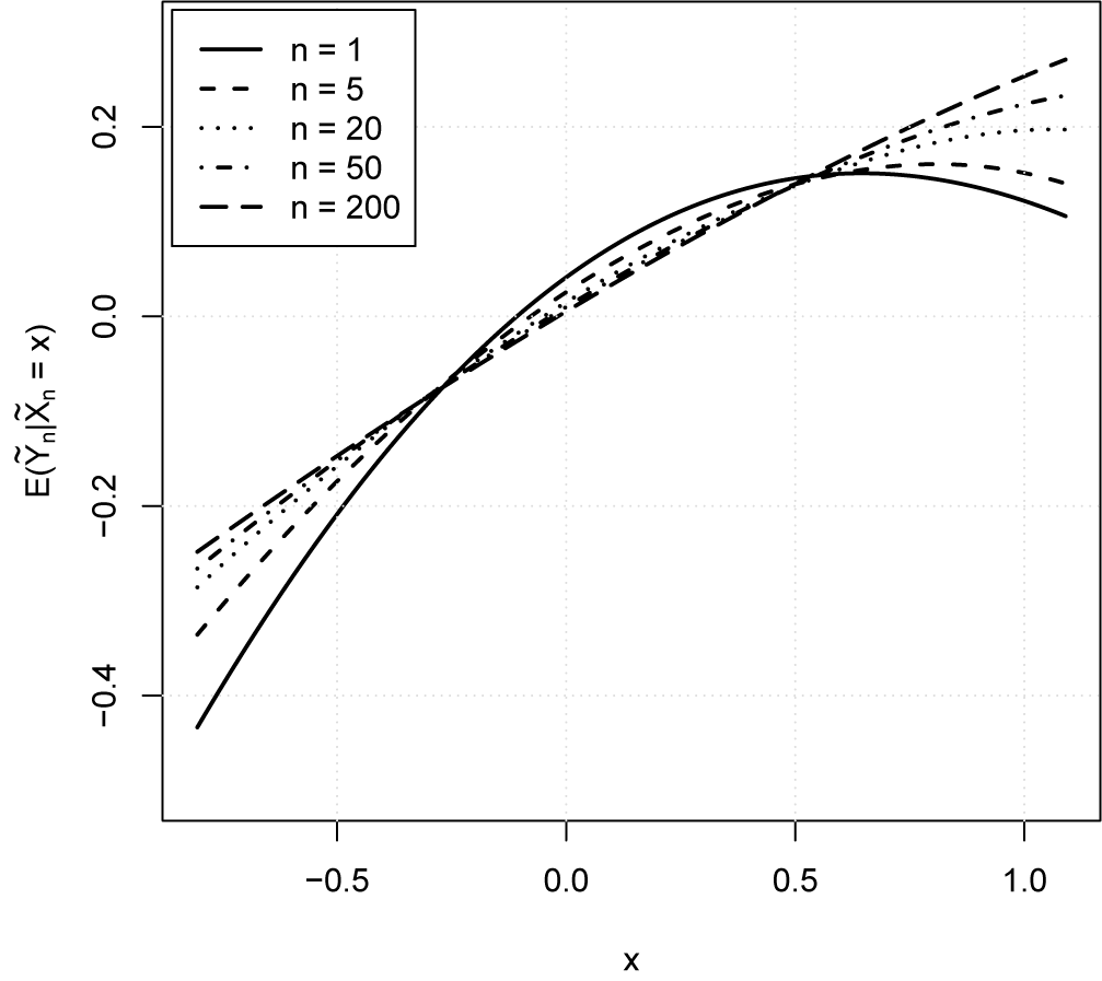
. In line with the developed theory, the conditional mean converges to a linear function.
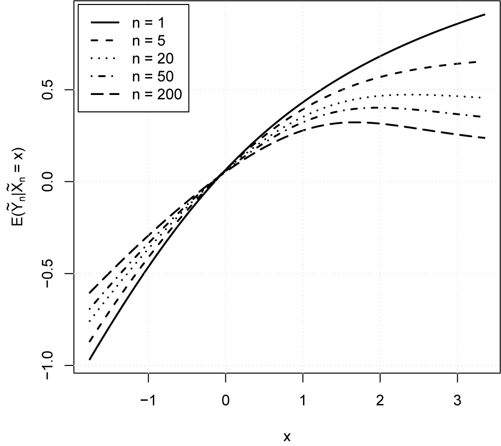
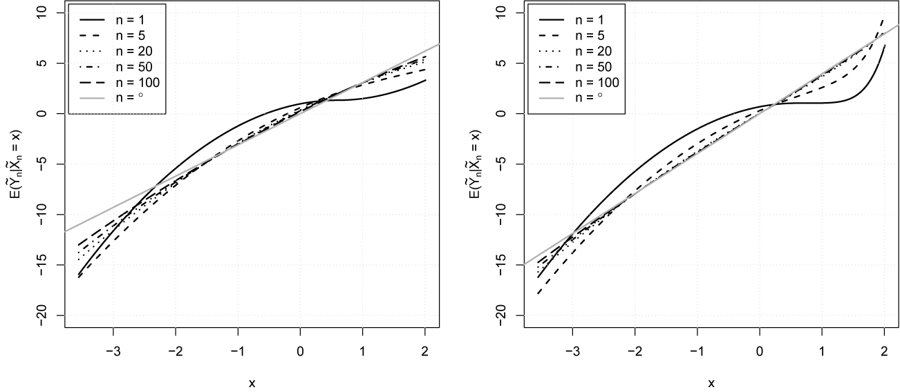
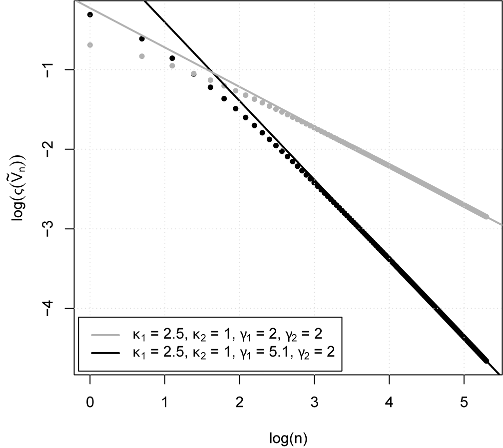
The conditional mean of the normalized sum as a function of the number of summands n when
 $V_1$
has a finite variance and a nonlinear conditional mean.
 $V_1 = (Y_1, X_1)$
follows a hyperbolic skewed-t with parameters
 $\lambda = -5$
and
 $\beta = (-2, 2)$
. The conditional mean converges to a linear function.

5.1.2 Rate of Convergence for Mixture Models
An interesting question is if there exist parameter values such that the conditions in equation (11) hold with
 $k \geq 2$
. Consider again the case
 $m = 1$
,
 $d = 1$
and assume that all parameters are fixed except for
 $\beta _Y$
. Given that
 $\mathbb {E}(V_1) = 0$
, the stochastic representation in (39) can be restated equivalently as
 $$ \begin{align} \begin{aligned} Y_1 &= \beta_Y(W - \mathbb{E} W) + \sqrt{W}Z_Y \\ X_1 &= \beta_X(W - \mathbb{E} W) + \sqrt{W}Z_X. \end{aligned} \end{align} $$
The third-order condition in equation (11) corresponding to
 $k = 2$
takes the form
 $\mathbb {E}(Y_1X_1^2) - \theta ^*\mathbb {E} X_1^3 = 0$
. This is a linear equation in
 $\beta _Y$
because
 $\theta ^* = \mathbb {E}(Y_1X_1)/\mathbb {E}(X_1^2)$
is also linear in
 $\beta _Y$
and the only solution is
 $\beta _Y = \sigma _{YX}\beta _X/\sigma _{XX}$
found by direct verification. According to equation (40), however, this choice of
 $\beta _Y$
turns the conditional mean into a linear function. As a consequence, in this case, the third-order moment condition in equation (11) guarantees linearity of the conditional mean.
The argument presented above is general and the same conclusion holds for any normal location-scale mixture for which the corresponding moments exist. Corollary 1, therefore, captures the rate of convergence for location-scale mixtures with finite variance. As far as
 $\delta $
is concerned, if the third moments of the marginals are finite,
 $\lambda < -3$
, then
 $\delta = 1$
can be used. If the third moments are unbounded, then the upper limit on
 $\delta $
is determined by the tail behavior of the marginals. For instance, in the case of the hyperbolic skewed-t, if we require
 $-3 \leq \lambda < -2$
to guarantee existence of second moments when the third moments are unbounded, the corresponding rate of decay is provided in Corollary 1 with
 $0 < \delta < \min (-\lambda - 2, 1)$
.
A way to engineer a model more flexible than the classical normal location-scale mixture is to change the tail behavior of the components in equation (41). Consider the next modification,
 $$ \begin{align} \begin{aligned} Y_1 &= \beta_Y(h(W) - \mathbb{E} h(W)) + \sqrt{h(W)}Z_Y \\ X_1 &= \beta_X(W - \mathbb{E} W) + \sqrt{W}Z_X, \end{aligned} \end{align} $$
where
 $h(x) = G^{-1}(F(x))$
in which F is the c.d.f. of W and G is the c.d.f. of a positive random variable. This construction is similar to the meta-Student-t distribution featuring different degrees of freedom for the marginals and the meta-elliptical distribution (Fang, Fang, and Kotz, Reference Fang, Fang and Kotz2002; Demarta and McNeil, Reference Demarta and McNeil2005). It is easy to see from the definition in (42) that the conditional mean is nonlinear even when
 $\beta _X = \beta _Y = 0$
,
 $$ \begin{align} \mathbb{E}(Y_1|X_1 = x) = x\frac{\sigma_{YX}}{\sigma_{XX}}\mathbb{E}\left(\frac{h(W_x)}{W_x}\right)^{1/2}, \end{align} $$
where
 $W_x$
denotes the conditional distribution
 $W|(X_1 = x)$
. At the same time, the multivariate law is symmetric when
 $\beta _X = \beta _Y = 0$
and the faster rate of convergence in Corollary 2 holds.
In a similar fashion, the equation
 $\mathbb {E}(Y_1X_1^2) - \theta ^*\mathbb {E} X_1^3 = 0$
is linear in
 $\beta _Y$
and can be used to determine
 $\beta _Y$
as a function of
 $\beta _X$
. The different tail behavior of the components provides more flexibility and, unlike the classical normal location-scale mixture, the moment condition for
 $k = 2$
can hold when the distribution is asymmetric and the conditional mean
 $\mathbb {E}(Y_1|X_1 = x)$
is nonlinear.
A similar argument is used in the construction in Section 5.2 in which the conditional mean is specified explicitly. A difficulty with the meta-mixture model in (43) is that the expectation on the right hand-side is not available in closed form.
5.1.3 Cross-Sectional Aggregation
The argument developed in Section 3.2 concerning portfolios can be illustrated in the following manner. Suppose
 $V_1 = (Y_1, X_1) \in \mathbb {R}^m\times \mathbb {R}^d$
in which the first m components are interpreted as basic assets and the last d components are interpreted as factors. The operator
 ${\mathbf {T}}_p$
takes the form
 $$\begin{align*}{\mathbf{T}}_p = \begin{pmatrix} {\mathbf{w}}^{\mathsf{T}} & \mathbf{0}_{1\times d}\\ \mathbf{0}_{d\times m} & \mathbf{I}_{d\times d} \\ \end{pmatrix}, \end{align*}$$
where
 ${\mathbf {w}} = (w_1, \ldots , w_m)$
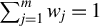
,
 $\sum _{j = 1}^m w_j = 1$
, denote portfolio weights. From the properties of the hyperbolic skewed-t distribution, it follows that the random vector
 ${\mathbf {T}}_p V_1$
has the same distribution with parameters
 ${\mathbf {T}}_p V_1 \in \mathrm {HSt}_\lambda ({\mathbf {T}}_p\mu , {\mathbf {T}}_p\beta , {\mathbf {T}}_p\Sigma {\mathbf {T}}_p^{\mathsf {T}}, \chi )$
 $$ \begin{align*} {\mathbf{T}}_p\mu = \begin{pmatrix} {\mathbf{w}}^{\mathsf{T}}\mu_Y \\ \mu_X \end{pmatrix},\qquad \beta = \begin{pmatrix} {\mathbf{w}}^{\mathsf{T}}\beta_Y \\ \beta_X \end{pmatrix},\qquad \Sigma = \begin{pmatrix} {\mathbf{w}}^{\mathsf{T}}\Sigma_{YY}{\mathbf{w}} & {\mathbf{w}}^{\mathsf{T}}\Sigma_{YX} \\ \Sigma_{XY}{\mathbf{w}} & \Sigma_{XX} \end{pmatrix}. \end{align*} $$
The relationship between the skewness parameters that results in a linear conditional mean can be readily expressed in terms of the weights and the parameters of the distribution of
 $V_1$
 $$\begin{align*}{\mathbf{w}}^{\mathsf{T}}(\beta_Y - \Sigma_{YX}\Sigma_{XX}^{-1}\beta_X) = 0. \end{align*}$$
Since this is a linear equation, clearly there are many portfolios with a linear conditional mean to the set of factors in
 $X_1$
even though all of the individual assets may have a nonlinear conditional mean to the same factor set.
5.1.4 Convergence to a Nonlinear Function
The next example concerns the case of a nonlinear limiting conditional mean in the case of infinite variance. Consider
 $(Y_1, X_1) \in \mathbb {R}\times \mathbb {R}$
and choose
 $\lambda = -1.75$
and
 $\beta = (0.001, 0.5)$
, which implies
 $\alpha = 1.75$
in equation (37). Both marginals have an infinite second moment and their limiting distribution is in the
 $\alpha $
-stable class. As noted in Theorem 4, in this situation, the limiting conditional mean may not be linear. Indeed, as illustrated in Figure 2, the conditional mean does not converge to a linear function.
The conditional mean of the normalized sum as a function of the number of summands n when
 $V_1$
has a nonlinear conditional mean and infinite variance.
 $V_1 = (Y_1, X_1)$
follows a hyperbolic skewed-t with parameters
 $\lambda = -1.75$
,
 $\beta = (0.001, 0.5)$
. The conditional mean does not converge to a linear function.

5.2 Examples of Different Rates of Convergence
Equation (11) provides the moment conditions that guarantee a given order of the convergence rate when the second moment is finite. In this section, our objective is to develop a bivariate example featuring a degree of analytic tractability in which the distribution of
 $X_1$
is asymmetric and remains fixed, the conditional mean is specified in closed form and its parameters can be chosen so that the moment conditions in equation (11) hold with
 $k \leq 2$
. Such an example is interesting also to illustrate that the moment conditions in (11) are not a trivial consequence of the CLT and the rate of convergence can be faster than the corresponding CLT rate for the same law.
Let
 $(Y, X) \in \mathbb {R}\times \mathbb {R}$
and assume X follows an asymmetric Laplace distribution with density
 $$\begin{align*}f_{X}(x) = \begin{cases} \dfrac{\kappa_1\kappa_2}{\kappa_1 + \kappa_2}\exp\{-\kappa_1(x - \mu)\}, & x \geq \mu \\[1em] \dfrac{\kappa_1\kappa_2}{\kappa_1 + \kappa_2}\exp\{-\kappa_2(\mu - x)\}, & x < \mu, \end{cases} \end{align*}$$
where
 $\kappa _1,\kappa _2> 0$
. Define Y by means of the stochastic representation
 $$ \begin{align} Y = g(X) + \epsilon, \end{align} $$
where
 $\epsilon $
and X are independent,
 $\epsilon $
is assumed to have finite variance, and the conditional mean is defined explicitly in the following way:
 $$ \begin{align} g(x) = \begin{cases} (x - \mu)^{\gamma_1}, & x \geq \mu \\ -(\mu - x)^{\gamma_2}, & x < \mu, \end{cases} \end{align} $$
where
 $\gamma _1,\gamma _2> 0$
.
The utility of this construction is that the expectations behind
 $\boldsymbol {\varsigma }$
and the corresponding moment conditions can be calculated analytically in closed form. The disadvantage is that although the distribution of X is infinitely divisible, that of Y may not be and in such a case
 $(Y, X)$
cannot be used to construct a Lévy process. Nevertheless, all results in the article can be restated without modification for the classical CLT scheme of sums of i.i.d. random vectors and the example is relevant (see Section 5.3).
Equation (45) and the relationship
 $\mathbb {E}(Ye^{iuX}) = \mathbb {E}(\mathbb {E}(Y|X)e^{iuX})$
are used to arrive at the next expressions for the ch.f. of X and all relevant moments
 $$ \begin{align} \phi_X(u) = \mathbb{E}(e^{iuX}) &= \frac{\kappa_1\kappa_2 e^{iu\mu}}{(\kappa_1 - iu)(\kappa_2 + iu)} \end{align} $$
 $$ \begin{align} \mathbb{E} (Ye^{iuX}) &= \frac{\kappa_1\kappa_2e^{iu\mu}}{\kappa_1 + \kappa_2}\left[\frac{\Gamma(\gamma_1 + 1)}{(\kappa_1 - iu)^{\gamma_1 + 1}} - \frac{\Gamma(\gamma_2 + 1)}{(\kappa_2 + iu)^{\gamma_2 + 1}}\right] \end{align} $$
 $$ \begin{align} \mathbb{E}(Xe^{iuX}) &= \frac{\kappa_1\kappa_2e^{iu\mu}}{\kappa_1 + \kappa_2}\left[\frac{1}{(\kappa_1 - iu)^{2}} - \frac{1}{(\kappa_2 + iu)^{2}}\right] + \mu\phi_X(u). \end{align} $$
The remaining moments together with
 $\theta ^*$
defined in equation (4) needed to compute
 $\boldsymbol {\varsigma }$
and the conditions in (11) are calculated by evaluating derivatives of (46)–(48) at
 $u = 0$
. Both X and Y need to be centered and, therefore, the location parameter is set to
 $\mu = -\mathbb {E} X = -(\kappa _2 - \kappa _1)/\kappa _1\kappa _2$
. The mean of Y needs to be subtracted as well inside the expectation in (47), which will result in a new term on the right side.
We note that the actual distribution of the residual in (44) is irrelevant in these calculations. The skewed Laplace distribution has exponential tails and the variance of
 $g(X)$
exists. The requirement for finite variance of
 $\epsilon $
is needed only to make sure the variance of Y is finite.
The conditional mean
 $\mathbb {E}(\widetilde {Y}_n | \widetilde {X}_n = x)$
is computed in two steps. First, repeating the steps behind the derivation of (5) we find that
 $$\begin{align*}\mathbb{E} (\widetilde{Y}_ne^{iu\widetilde{X}_n}) = n^{1/2}\mathbb{E} (Y e^{in^{-1/2}u X})\left[\phi_X(n^{-1/2}u)\right]^{n-1}. \end{align*}$$
Second, we use equation (38) and apply the FFT to the function
 $\mathbb {E} (\widetilde {Y}_ne^{iu\widetilde {X}_n})$
to evaluate numerically the conditional mean. The left plot in Figure 3 shows how the conditional mean changes as a function of n with parameter values
 $\kappa _1 = 2.5$
,
 $\kappa _2 = 1$
, and
 $\gamma _1 = \gamma _2 = 2$
. The distribution of X is skewed to the left and the grid for x ranges from the 1% quantile to the 99% quantile of X. With these parameter values, the third-order moment condition in (11) does not hold. The rate of convergence in Corollary 1 is expected to hold for this situation.
The conditional mean of the normalized sum as a function of the number of summands n with parameters
 $\kappa _1 = 2.5$
,
 $\kappa _2 = 1$
, and
 $\gamma _1 = \gamma _2 = 2$
(left) and
 $\kappa _1 = 2.5$
,
 $\kappa _2 = 1$
,
 $\gamma _1 = 5.1$
, and
 $\gamma _2 = 2$
(right). The plot on the right illustrates a faster rate of convergence because the choice of parameters ensures that the third-order moment condition in (11) is satisfied. The grid on the horizontal axis starts at the 1% quantile and ends at the 99% quantile of the distribution of X.

Next, we find a new value for
 $\gamma _1$
by numerically solving the third-order condition in (11),
 $\mathbb {E}[(Y - \theta ^*X)X^2] = 0$
. Conditional on the other parameters, the solution is
 $\gamma _1^* = 5.1> \gamma _1 = 2$
which is intuitive given that g needs to steepen to compensate for the lighter right tail of X in order for the moment condition to hold. The right plot in Figure 3 illustrates this case. Even though the conditional mean g is now more curved, the rate of convergence to the asymptotic linear case is visually faster as expected based on Theorem 2.
The actual rate of convergence in these two cases is estimated formally in the following way. The log-transform applied to both sides of (14) leads to the next asymptotic relationship for large n
 $$ \begin{align} \log\left(\boldsymbol{\varsigma}(\widetilde{V}_n)\right) = a + \frac{1 - r}{2}\log(n) + \varepsilon, \end{align} $$
where
 $r = k + \delta $
in which k denotes the corresponding moment order. The left side is calculated numerically from the definition in (7) with
 $\psi (u) = \exp (-u^2/2)$
in which we set
 $\theta = \theta ^*$
. The quantity in the absolute value is calculated using (5) and the explicit representations in (47) and (48). Finally, the maximization of the absolute value is conducted numerically over a grid whose size is dictated by the fast decay of
 $\psi (u)$
.
Both sides of (49) are evaluated for
 $n = 1,2,\dots , 200$
but the coefficients are estimated from the data with
 $n \geq 100$
because the relationship is asymptotic in theory. For the first set of parameters, we find that
 $\hat {r}_{\mathrm {slow}} = 1.99$
with
 $\hat {k}_{\mathrm {slow}} = 1$
and for the second set of parameters,
 $\hat {r}_{\mathrm {fast}} = 2.98$
with
 $\hat {k}_{\mathrm {fast}} = 2$
, which is exactly as expected. The estimated relationships together with the data are presented in Figure 4.
Estimated rates of convergence for a distribution that meets the third-order moment condition in (11) (in black) and for one that does not (in gray). In line with theory, the estimated rates of convergence are
 $\hat {r}_{\mathrm {fast}} = 2.98$
with
 $\hat {k}_{\mathrm {fast}} = 2$
for the data in black and
 $\hat {r}_{\mathrm {slow}} = 1.99$
with
 $\hat {k}_{\mathrm {slow}} = 1$
for the data in gray.

Finally, we compare the rate of convergence in the CLT to the rates above. It is important to note that the rate of convergence in the classical CLT depends on some additional properties of the distribution of
 $\epsilon $
in (44), while the rates computed above do not depend on
 $\epsilon $
. For example, in line with the conditions in (33), to reach the faster rate
 $\hat {r}_{\mathrm {fast}}$
one would need to require,
 $$\begin{align*}\mathbb{E}(Y^{\ell}X^m) = \mathbb{E}(Z_y^{\ell}Z_x^m), \end{align*}$$
where
 $\ell ,m$
are positive integers or zero such that
 $\ell + m = 1,2,3$
and
 $(Z_y, Z_x)$
has a bivariate Gaussian distribution.Footnote
10
Clearly, these conditions imply symmetry for the marginals
 $\mathbb {E} Y^3 = \mathbb {E} X^3 = 0$
and X is asymmetric by construction while the symmetry of Y depends on the properties of
 $\epsilon $
. In this particular example, the rate behind
 $\hat {r}_{\mathrm {fast}}$
is not attainable for the vector
 $(Y, X)$
in the CLT, for example, in the Berry–Esseen setup, but even if
 $X \overset {\scriptscriptstyle d}{=} -X$
, then the CLT rate would depend on the properties of
 $\epsilon $
. As a result, the limit theorems for the conditional mean developed in this article are not a simple consequence of the CLT. Rather, they can be viewed as a separate class of results specialized for conditional means.
5.3 Beyond Lévy Processes
The focus of the article is the assumption that the data generating process follows a multivariate Lévy process. We take advantage of the property that its increments over time intervals of the equal length are i.i.d. random vectors. The proofs do not rely on the infinite divisibility of the increments and the rates of decay in Theorems 2–4 hold for sequences of i.i.d. random vectors as well.
From the standpoint of applications of discrete time processes, a more appealing setup is that of independent non-identically distributed random vectors. The framework developed in this article can handle this extension. Next, we provide a pair of assumptions similar to Assumptions 1 and 2.
Assumption 1‡. The sequence
 $V_1, V_2,\dots $
consists of independent non-identically distributed random vectors,
 $V_{j} = (Y_{j}, X_{j}) \in \mathbb {R}\times \mathbb {R}^d$
with
 $\mathbb {E}(V_{j}) = 0$
,
 $\mathbb {E}\|V_j\|_2^2 < \infty $
, and
 $\mathbb {E}[V_jV_j^{\mathsf {T}}] = {\mathbf {C}}$
for all j.
Assumption 2‡. The following moment conditions hold for all
 $j:$
 $$ \begin{align} \mathbb{E}\left((Y_{j} - X_{j}^{\mathsf{T}} \theta^*)X^{\nu}_{j}\right) &= 0, \quad \forall \nu\colon |\nu| \leq k \end{align} $$
 $$ \begin{align} \mathbb{E}\left(|Y_{j} - X_{j}^{\mathsf{T}}\theta^*|\|X_{j}\|_1^{r}\right) &\leq D < \infty, \end{align} $$
where
 $k \geq 1$
is an integer,
 $\nu $
denotes a multi-index,
 $r = k + \delta $
with
 $\delta \in (0, 1]$
, and
 $\theta ^* = {\mathbf {C}}_{XX}^{-1}{\mathbf {C}}_{YX}$
exists in which the index notation identifies the corresponding blocks in
 ${\mathbf {C}}$
.
Both assumptions include moment conditions holding across all members of the sequence in the same way. Such a degree of uniformity is not required in the proof but simplifies the notation and makes the connection with the i.i.d. case easier to understand. The rate of decay is provided in the following theorem.
Theorem 5. Under Assumptions 1‡ and 2‡ ,
 $$ \begin{align} \boldsymbol{\varsigma}\left(n^{-1/2}\sum_{j = 1}^nV_{j}\right) \leq C_{r}n^{-\frac{r + 1}{2}}\sum_{j = 1}^n\boldsymbol{b}_{r}(V_{j}), \end{align} $$
where
 $r \geq 1$
,
 $C_r = \sup _u\left \lVert u\right \rVert _1^r\psi (u)$
. Furthermore, the next bound holds
 $$ \begin{align} \sum_{j = 1}^n\boldsymbol{b}_{r}(V_{j}) \leq nA_\delta \frac{\Gamma(\delta + 1)}{\Gamma(r + 1)}D, \end{align} $$
where the notation is as in Theorem 2.
If the elements of the sequence are i.i.d., then
 $\boldsymbol {b}_r(V_1) = \boldsymbol {b}_r(V_j)$
for all j and it is easy to see how equations (52) and (53) turn into equations (14) and (15). Combining both inequalities in Theorem 5 indicates the rate of decay is similar to the one in Theorem 2. The main difference is the increase in the scaling constant. The similarity in the rate of decay in the two theorems follows from the conditions in equation (50) holding uniformly for all j.
Relaxing the assumption of independence is a lot more challenging and is beyond the scope of this article but it is important for applications in economics and finance (Rachev and Mittnik, Reference Rachev and Mittnik2000; Cont and Tankov, Reference Cont and Tankov2003; Stock and Watson, Reference Stock, Watson, Clements and Hendry2011). From the viewpoint of both theory and practice, one important general relaxation includes
 $V_1, V_2, \dots $
forming a multivariate martingale difference sequence. The CLT holds in this case subject to certain regularity conditions and rate-of-convergence results in terms of the uniform metric in discrete and continuous time can be found in Butzer, Hahn, and Roeckerath (Reference Butzer, Hahn and Roeckerath1983), Haeusler (Reference Haeusler1988), Račkauskas (Reference Račkauskas1991), and Mourrat (Reference Mourrat2013).
Another important relaxation is weak dependence which implies the correlation between the elements of the sequence decreases as the time lag increases. Rate-of-convergence results in the CLT setting for weakly dependent random variables are available, for example, in Tikhomirov (Reference Tikhomirov1991, Reference Tikhomirov1994).
Given that subject to certain regularity conditions there is a CLT result in both settings, the conditional expectations of a properly normalized sum converge to a linear function. It is a future topic of research to study the rate-of-convergence problem for conditional means in these settings and to understand how the rates compare to the corresponding CLT rates available in the academic literature.
6 CONCLUSION
Linear models have a central place in empirical asset pricing in the field of finance and are widely considered a successful framework. From an econometric perspective, however, the assumption of linearity is not commonly tested for adequacy. In this article, we propose an asymptotic probabilistic argument which indicates that the model error may decline for lower frequency return data due to temporal aggregation. Apart from the field of finance, the results in the article may be useful in other domains in which temporal aggregation plays a role.
If the return process of the joint vector of the dependent and the independent variables follows a multivariate Lévy process with finite second moments, we prove that the conditional expectation of the dependent variable converges to a linear function as the return frequency declines and the rate of convergence is bounded by a power law. The rate of convergence is determined by a set of moment conditions with an econometric interpretation. If the dependent variable is a return of a portfolio, the additional cross-sectional aggregation can improve the rate of convergence, which indicates that the model error of the linear framework can be smaller for portfolios than individual stocks.
Relaxing the assumptions of finite second moments leads to a non-trivial extension of the asymptotic results. Even though this case is of limited practical significance for the field of finance, it is of theoretical interest. As expected from general limit theory, the index of stability of the increments of the Lévy process appears in the exponent of the power law. Also, the limiting stable law appears explicitly in the scaling constant and in the moment conditions that play a role in the rate of convergence.
Finally, from a probabilistic perspective, the developed theory and the numerical examples indicate that the results presented in the article are not a simple consequence of the CLT and the GCLT. Rather, they can be viewed as a separate class of limit theorems specialized for conditional expectations.
A APPENDIX
Proof of Theorem 1
Set
 $\Delta t = \tau $
and assume
 $\mathbb {E}(Y_{\tau }|X_{\tau }) \overset {\scriptscriptstyle \mathit {a.s.}}{=} X_{\tau }^{\mathsf {T}}\theta $
for some fixed
 $\theta $
. We repeat the arguments behind equation (5)
 $$ \begin{align*} \Bigl|\mathbb{E}(Y_{n\tau} - X_{n\tau}^{\mathsf{T}} \theta)e^{iu^{\mathsf{T}} X_{n\tau}} \Bigr| &= \left| \sum_{k = 1}^n\mathbb{E}\left[(\Delta Y_{k} - \Delta X_{k}^{\mathsf{T}} \theta)e^{i u^{\mathsf{T}} \Delta X_{k}}\right]\mathbb{E} e^{iu^{\mathsf{T}} \sum_{j \not = k}\Delta X_{j}}\right| \\ &\leq \sum_{k = 1}^n\left|\mathbb{E}(\Delta Y_{k} - \Delta X_{k}^{\mathsf{T}} \theta)e^{i u^{\mathsf{T}} \Delta X_{k}}\right|\Bigl|\mathbb{E} e^{iu^{\mathsf{T}} \sum_{j \not = k}\Delta X_{j}}\Bigr|\\ &\leq \sum_{k = 1}^n\left|\mathbb{E}(\Delta Y_{k} - \Delta X_{k}^{\mathsf{T}} \theta)e^{i u^{\mathsf{T}} \Delta X_{k}}\right|\\ &= n\left|\mathbb{E}(Y_{\tau} - X_{\tau}^{\mathsf{T}} \theta)e^{i u^{\mathsf{T}} X_{\tau}}\right|. \end{align*} $$
If
 $\mathbb {E}(Y_{\tau } - X_{\tau }^{\mathsf {T}} \theta )e^{i u^{\mathsf {T}} X_{\tau }} = 0$
for all
 $u \in \mathbb {R}^d$
, then the left side vanishes for all u. As a result,
 $\mathbb {E}(Y_{n\tau }|X_{n\tau }) \overset {\scriptscriptstyle \mathit {a.s.}}{=} X_{n\tau }^{\mathsf {T}}\theta $
for any integer
 $n \geq 1$
.
By Miller (Reference Miller1978, Thm. 3.1), the conditional mean
 $\mathbb {E}[Y_\tau |X_\tau ]$
is linear if and only if the following relationship holds for the derivatives of the ch.f. of
 $V_\tau $
denoted by
 $\phi _{V_\tau }(z, u) = \mathbb {E} e^{izY_\tau + iu^{\mathsf {T}} X_\tau }$
:
 $$ \begin{align} \partial_z\phi_{V_\tau}(0, u) = \sum_{i = 1}^d\theta_i\partial_{u_i}\phi_{V_\tau}(0, u), \end{align} $$
in which
 $\partial _x$
denotes the first derivative with respect to the variable x. By assumption, equation (A.1) holds for some fixed
 $\theta $
.
Next, from the definition of a Lévy process, the ch.f. equals
 $\phi _{V_\tau }(z, u) = (\phi _{V_{\tau /k}}(z, u))^k$
, where
 $k \geq 1$
is an integer. Computing the derivatives on both sides of (A.1) results in
 $$ \begin{align*} k(\phi_{V_{\tau/k}}(0, u))^{k-1}\partial_z\phi_{V_{\tau/k}}(0, u) = \sum_{i = 1}^d\theta_ik(\phi_{V_{\tau/k}}(0, u))^{k-1}\partial_{u_i}\phi_{V_{\tau/k}}(0, u). \end{align*} $$
The term
 $k(\phi _{V_{\tau /k}}(0, u))^{k-1}$
is common on both sides and, therefore, (A.1) holds for
 $V_{\tau /k}$
with the same
 $\theta $
. From here, we conclude that
 $\mathbb {E}(Y_{\tau /k}|X_{\tau /k}) \overset {\scriptscriptstyle \mathit {a.s.}}{=} X_{\tau /k}^{\mathsf {T}}\theta $
for any integer
 $k \geq 1$
.
Combining both statements, we conclude that
 $\mathbb {E}(Y_{n\tau /k}|X_{n\tau /k}) \overset {\scriptscriptstyle \mathit {a.s.}}{=} X_{n\tau /k}^{\mathsf {T}}\theta $
, where n and k are positive integers. As a final step, choose an arbitrary
 $t \geq 0$
. Then,
 $t/\tau $
can be approximated arbitrarily well by a rational number of the form
 $n/k$
, where n and k are positive integers. Thus, t can be represented in the form
 $t = n\tau /k$
and the result follows from the convergence
 $V_{n\tau /k} \to V_t$
in distribution.
Lemma A.1. Suppose that
 $V = (Y,X) \in \mathbb {R}\times \mathbb {R}^d$
is a zero-mean random vector with
 $\mathbb {E}\left \lVert V\right \rVert _1 < \infty $
. Define
 $$ \begin{align*}\nonumber \boldsymbol{\varsigma}(V) &= \inf_{\theta}\boldsymbol{\varsigma}^\theta(V) \\\nonumber \boldsymbol{\varsigma}^\theta(V) &= \sup_{u\in \mathbb{R}^{d}}\psi(u)\left|\mathbb{E}(Y - X^{\mathsf{T}}\theta)e^{iu^{\mathsf{T}} X}\right|, \end{align*} $$
where
 $\psi (u)> 0$
is a ch.f. of a symmetric random vector. The functional
 $\boldsymbol {\varsigma }(V)$
is nonnegative and equals zero if and only if
 $\mathbb {E}(Y|X) = X^{\mathsf {T}}\theta $
almost surely for some
 $\theta $
.
Proof. For any fixed
 $\theta $
and any
 $u \in \mathbb {R}^d$
,
 $$ \begin{align*} \psi(u)\left|\mathbb{E}(Y - X^{\mathsf{T}}\theta)e^{iu^{\mathsf{T}} X}\right| \leq \max(1, \|\theta\|_\infty)\mathbb{E}\left\lVert V\right\rVert_1 < \infty. \end{align*} $$
Therefore, under the assumptions in the lemma,
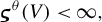 $\boldsymbol {\varsigma }^\theta (V) < \infty ,$
and, as a consequence,
 $\boldsymbol {\varsigma }(V)$
is bounded as well.
If
 $\mathbb {E}(Y|X) = X^{\mathsf {T}}\theta $
almost surely for some
 $\theta $
, then by Bierens (Reference Bierens1982, Thm. 1), it follows that
 $\mathbb {E}(Y - X^{\mathsf {T}}\theta )e^{iu^{\mathsf {T}} X} = 0$
for all
 $u \in \mathbb {R}^d$
. As a result,
 $\boldsymbol {\varsigma }(V) = 0$
.
In the opposite direction, if
 $\boldsymbol {\varsigma }^\theta (V) = 0$
for some
 $\theta $
, then
 $\mathbb {E}(Y - X^{\mathsf {T}}\theta )e^{iu^{\mathsf {T}} X} = 0$
for all
 $u \in \mathbb {R}^d$
because
 $\psi (u)> 0$
. This is necessary and sufficient for
 $\mathbb {E}(Y|X) = X^{\mathsf {T}}\theta $
almost surely by Bierens (Reference Bierens1982, Thm. 1).
Lemma A.2. Suppose that
 $V = (Y,X) \in \mathbb {R}\times \mathbb {R}^d$
is a zero-mean random vector such that
 $\mathbb {E}|Y - X^{\mathsf {T}}\theta ^*|\left \lVert X\right \rVert _1^r < \infty $
, where
 $r = k + \delta $
,
 $k\geq 1$
is an integer,
 $0 < \delta \leq 1$
, and
 $\theta ^* = (\mathbb {E}[XX^{\mathsf {T}}])^{-1}\mathbb {E}[XY]$
. Suppose also that the moment conditions
 $\mathbb {E}(Y - X^{\mathsf {T}}\theta ^*)X^{\nu } = 0, \forall \nu \colon |\nu | \leq k$
hold, where
 $\nu $
is a multi-index. Define
 $$ \begin{align*} \boldsymbol{\zeta}_r(V) = \sup_{g \in \mathcal{G}}\left|\mathbb{E}(Y - X^{\mathsf{T}}\theta^*)g(X)\right|, \end{align*} $$
where
 $$ \begin{align} \mathcal{G} = \left\{g\colon\mathbb{R}^{d} \rightarrow \mathbb{C}, \left|\partial^\nu g(u) - \partial^{\nu} g(v)\right| \leq \left\lVert u - v\right\rVert_1^\delta, \delta \in (0,1], \forall \nu\colon |\nu| = k\right\}. \end{align} $$
The following bound holds:
 $$ \begin{align*} \boldsymbol{\zeta}_r(V) \leq \frac{\Gamma(\delta + 1)}{\Gamma(r + 1)}\mathbb{E}\left(|Y - X^{\mathsf{T}}\theta^*|\left\lVert X\right\rVert_1^{r}\right). \end{align*} $$
Proof. The construction is similar to the construction of zeta distances in the theory of probability metrics (see Rachev et al., Reference Rachev, Klebanov, Stoyanov and Fabozzi2013, Chap. 4.4, Lemma 15.3.6, and Remark 15.4.2). The functions from the class
 $\mathcal {G}$
can be written in terms of their Taylor expansion at
 $x = 0$
(see, e.g., Cartan, Reference Cartan1971)
 $$ \begin{align*} \begin{aligned} g(x) &= \sum_{|\nu| \leq k - 1}\frac{\partial^{\nu}g(0)}{\nu!}x^{\nu} + k\sum_{|\nu| = k}\frac{x^{\nu}}{\nu!}\int_{0}^{1}(1 - \tau)^{k-1}\partial^{\nu}g(\tau x)d\tau \\ &= \sum_{|\nu| \leq k}\frac{\partial^{\nu}g(0)}{\nu!}x^{\nu} + k\sum_{|\nu| = k}\frac{x^{\nu}}{\nu!}\int_{0}^{1}(1 - \tau)^{k-1}(\partial^{\nu}g(\tau x) - \partial^{\nu}g(0))d\tau, \end{aligned} \end{align*} $$
where
 $\nu ! = \nu _1!\nu _2!\ldots \nu _d!$
. For the expectation, we find
 $$ \begin{align*} \begin{aligned} \mathbb{E}(Y - X^{\mathsf{T}}\theta)g(X) &= \mathbb{E}\left[(Y - X^{\mathsf{T}}\theta)\left(\sum_{|\nu| \leq k}\frac{\partial^{\nu}g(0)}{\nu!}X^{\nu} + R_{k}(X)\right)\right]. \end{aligned} \end{align*} $$
The moment conditions
 $\mathbb {E}(Y - X^{\mathsf {T}}\theta )X^{\nu } = 0, \forall \nu \colon |\nu | \leq k$
for some fixed
 $\theta $
are necessary for the existence of
 $\sup _{g \in \mathcal {G}}\left |\mathbb {E}(Y - X^{\mathsf {T}}\theta )g(X)\right |$
. To see why, assume the contrary. If
 $\mathbb {E}(Y - X^{\mathsf {T}}\theta )X^{\nu } \not = 0$
for some
 $\nu \colon |\nu | \leq k$
, then it is possible to find a function in the class
 $\mathcal {G}$
with a sufficiently large derivative
 $\partial ^{\nu }g(0)$
in absolute value so that the corresponding term in the expansion becomes arbitrarily large in absolute value.
Consider the first two terms. If
 $k = 0$
, then
 $\mathbb {E}(Y - X^{\mathsf {T}}\theta ) = 0$
is satisfied for any
 $\theta $
because by assumption
 $V = (Y,X)$
is zero-mean. If
 $k = 1$
, the moment condition becomes
 $\mathbb {E}(Y - X^{\mathsf {T}}\theta )X = 0$
and it is satisfied at
 $\theta = \theta ^*$
by design. For
 $k> 1$
, the corresponding moment condition must hold at
 $\theta = \theta ^*$
. Thus, the necessary conditions for boundedness become
 $\mathbb {E}(Y - X^{\mathsf {T}}\theta ^*)X^{\nu } = 0, \forall \nu \colon |\nu | \leq k$
.
Denote the term which does not vanish by I,
 $$ \begin{align*} I = \mathbb{E}\left(\left(Y - X^{\mathsf{T}}\theta^*\right)k\sum_{|\nu| = k}\frac{X^{\nu}}{\nu!}\int_{0}^{1}(1 - \tau)^{k-1}(\partial^{\nu}g(\tau X) - \partial^{\nu}g(0))d\tau\right). \end{align*} $$
The following inequalities hold:
 $$ \begin{align*} |I| &\leq \mathbb{E}\left(\left|Y - X^{\mathsf{T}}\theta^*\right|\sum_{|\nu| = k}k\frac{|X|^{\nu}}{\nu!}\int_{0}^{1}(1 - \tau)^{k-1}\left|\partial^{\nu}g(\tau X) - \partial^{\nu}g(0)\right|d\tau\right)\\ &\leq \mathbb{E}\left(\left|Y - X^{\mathsf{T}}\theta^*\right|\sum_{|\nu| = k}k\frac{|X|^{\nu}}{\nu!}\int_{0}^{1}(1 - \tau)^{k-1}\left\lVert\tau X\right\rVert_1^{\delta}d\tau\right)\\ &= \mathbb{E}\left(\left|Y - X^{\mathsf{T}}\theta^*\right|\sum_{|\nu| = k}k\frac{|X|^{\nu}}{\nu!}\left\lVert X\right\rVert_1^{\delta}\frac{\Gamma(k)\Gamma(\delta + 1)}{\Gamma(k + \delta + 1)}\right)\\ &= \mathbb{E}\left(\left|Y - X^{\mathsf{T}}\theta^*\right|\sum_{|\nu| = k}k!\frac{|X|^{\nu}}{\nu!}\left\lVert X\right\rVert_1^{\delta}\frac{\Gamma(\delta + 1)}{\Gamma(k + \delta + 1)}\right) \\ &= \frac{\Gamma(\delta + 1)}{\Gamma(k + \delta + 1)}\mathbb{E}\left(\left|Y - X^{\mathsf{T}}\theta^*\right|\left(\sum_{j = 1}^{d}|X_{j}|\right)^{k}\left\lVert X\right\rVert_1^{\delta}\right)\\ &=\frac{\Gamma(\delta + 1)}{\Gamma(k + \delta + 1)}\mathbb{E}\left(|Y - X^{\mathsf{T}}\theta^*|\left\lVert X\right\rVert_1^{k + \delta}\right), \end{align*} $$
in which we take advantage of the multinomial theorem,
 $\sum _{|\nu | = k}\frac {k!}{\nu !}|X|^{\nu } = (\sum _{j=1}^d|X_j|)^k$
.
As a result, for any
 $g\in \mathcal {G}$
,
 $$ \begin{align*}\left|\mathbb{E}(Y - X^{\mathsf{T}}\theta^*)g(X_t)\right| = |I| \leq \frac{\Gamma(\delta + 1)}{\Gamma(k + \delta + 1)}\mathbb{E}\left(|Y - X^{\mathsf{T}}\theta^*|\left\lVert X\right\rVert_1^{k + \delta}\right),\end{align*} $$
and the proof is completed after taking the supremum over all
 $g \in \mathcal {G}$
.
Lemma A.3. Suppose that
 $V = (Y,X) \in \mathbb {R}\times \mathbb {R}^d$
is a zero-mean random vector and that the moment conditions in Lemma A.2 hold. Define
 $$ \begin{align*}\nonumber \boldsymbol{b}_r(V) = \sup_{u\in \mathbb{R}^{d}}\left\lVert u\right\rVert_1^{-r}\left|\mathbb{E}(Y - X^{\mathsf{T}}\theta)e^{iu^{\mathsf{T}} X}\right|,\quad r \geq 1. \end{align*} $$
The functional is unbounded if
 $\theta \not = \theta ^*$
. The next upper bound holds
 $$ \begin{align} \boldsymbol{b}_r(V) \leq A_\delta\boldsymbol{\zeta}_r(V), \end{align} $$
where
 $r = k + \delta $
,
 $k\geq 1$
is an integer,
 $0 < \delta \leq 1,$
and
 $A_\delta = \sup _{y \in \mathbb {R}} |y|^{-\delta }|e^{iy} - 1|$
. Finally, the following scaling property holds:
 $$ \begin{align*} \boldsymbol{b}_r(aV) = |a|^{r + 1}\boldsymbol{b}_{r}(V), \end{align*} $$
where
 $a \in \mathbb {R}$
is a constant.
Proof. We show that
 $\boldsymbol {b}_{r}(V)$
can be represented as a special case of the
 $\boldsymbol {\zeta }_{r}(V)$
functional in which we consider a sub-class of
 $\mathcal {G}$
. Choose
 $h_u(x) = \exp (iu^{\mathsf {T}} x)/\left \lVert u\right \rVert _1^{k + \delta }$
, where
 $u\in \mathbb {R}^d$
, and a multi-index
 $\nu $
such that
 $|\nu | = k$
. A direct calculation shows that
 $$ \begin{align*} \begin{aligned} \left|\partial^{\nu} h_u(x) - \partial^{\nu} h_u(y)\right| &\leq \frac{|u|^{\nu}|e^{iu^{\mathsf{T}} x} - e^{iu^{\mathsf{T}} y}|}{\left\lVert u\right\rVert_1^{k+\delta}}\\ &\leq \frac{|u|^{\nu}|e^{iu^{\mathsf{T}}(x-y)} - 1|}{\left\lVert u\right\rVert_1^{k+\delta}}, \end{aligned} \end{align*} $$
where
 $|u|^\nu = \prod _{j=1}^d|u_j|^{\nu _j}$
. We divide both sides by
 $\left \lVert x - y\right \rVert _1^{\delta }$
and we obtain
 $$ \begin{align*} \frac{1}{\left\lVert x - y\right\rVert_1^{\delta}}\left|\partial^{\nu} h_u(x) - \partial^{\nu} h_u(y)\right| &\leq\frac{|u|^{\nu}|e^{iu^{\mathsf{T}}(x-y)} - 1|}{\left\lVert u\right\rVert_1^{k+\delta}\left\lVert x - y\right\rVert_1^{\delta}}\\ &\leq \frac{\left\lVert u\right\rVert_1^k|e^{iu^{\mathsf{T}} (x-y)} - 1|}{\left\lVert u\right\rVert_1^{k+\delta}\left\lVert x - y\right\rVert_1^{\delta}}\\ &= \frac{|e^{iu^{\mathsf{T}}(x-y)} - 1|}{\left\lVert u\right\rVert_1^{\delta}\left\lVert x - y\right\rVert_1^{\delta}}, \end{align*} $$
which uses the fact that
 $\prod _j|u_j|^{\nu _j}\leq (\sum _j|u_j|)^k$
following from the multinomial theorem. The right hand-side can be increased further using
 $$ \begin{align*} \left|\sum_{i = 1}^d u_i(x_i - y_i)\right| \leq \sum_{i = 1}^d |u_i||x_i - y_i| \leq \left(\sum_{i = 1}^d|u_i|\right) \left(\sum_{j = 1}^d|x_j - y_j|\right). \end{align*} $$
We obtain
 $$ \begin{align*} \frac{1}{\left\lVert x-y\right\rVert_1^{\delta}}\left|\partial^{\nu} h_u(x) - \partial^{\nu} h_u(y)\right| \leq \frac{|e^{iu^{\mathsf{T}}(x-y)} - 1|}{|u^{\mathsf{T}}(x-y)|^\delta} \leq \sup_{z \in \mathbb{R}}\frac{|e^{iz} - 1|}{|z|^{\delta}} = A_\delta. \end{align*} $$
It is easy to see that
 $A_\delta < \infty $
. As a result, we have proved the following inclusion:
 $$ \begin{align*}\mathcal{H}=\left\{h\colon \mathbb{R}^{d} \rightarrow \mathbb{C}, h(x) = \frac{1}{A_\delta} \frac{e^{iu^{\mathsf{T}} x}}{\left\lVert u\right\rVert_1^{k + \delta}}\right\} \subset \mathcal{G}\end{align*} $$
and, as a consequence, the next inequality holds with
 $\theta = \theta ^*$
 $$ \begin{align*} \frac{1}{A_\delta} \sup_{u\in \mathbb{R}^{d}}\left\lVert u\right\rVert_1^{-k-\delta}\left|\mathbb{E}(Y - X^{\mathsf{T}}\theta^*)e^{iu^{\mathsf{T}} X}\right| &= \sup_{h \in \mathcal{H}}\left|\mathbb{E}(Y - X^{\mathsf{T}}\theta^*)h(X)\right| \\ &\leq \sup_{g \in \mathcal{G}}\left|\mathbb{E}(Y - X^{\mathsf{T}}\theta^*)g(X)\right|, \end{align*} $$
which completes the proof of the inequality in equation (A.3).
If
 $\theta \not = \theta ^*$
, then
 $\boldsymbol {b}_r(V)$
is unbounded. The argument is the same as the one in the proof of Lemma A.2. For any
 $\theta \not = \theta ^*$
, the moment
 $\mathbb {E}(Y - X^{\mathsf {T}}\theta )X \not = 0$
. The corresponding term in the Taylor expansion of
 $h_u(x)$
then becomes unbounded when
 $\left \lVert u\right \rVert _1 \rightarrow 0$
.
The scaling property follows easily from the definition. Let
 $\theta = \theta ^*$
, then
 $$ \begin{align*} \sup_{u\in \mathbb{R}^{d}}\left\lVert u\right\rVert_1^{-r}\left|\mathbb{E}(aY - aX^{\mathsf{T}}\theta)e^{iu^{\mathsf{T}} aX}\right| &= |a|\sup_{u\in \mathbb{R}^{d}}\left\lVert u\right\rVert_1^{-r}\left|\mathbb{E}(Y - X^{\mathsf{T}}\theta)e^{iau^{\mathsf{T}} X}\right|\\ & = |a|\sup_{au\in \mathbb{R}^{d}}|a|^r\left\lVert au\right\rVert_1^{-r}\left|\mathbb{E}(Y - X^{\mathsf{T}}\theta)e^{iau^{\mathsf{T}} X}\right|\\ & = |a|^{r+1}\sup_{v\in \mathbb{R}^{d}}\left\lVert v\right\rVert_1^{-r}\left|\mathbb{E}(Y - X^{\mathsf{T}}\theta)e^{iv^{\mathsf{T}} X}\right|. \end{align*} $$
Lemma A.4. Suppose
 $V_1, V_2, \ldots , V_n$
are independent copies of
 $V = (Y, X)$
. Then,
 $$ \begin{align*} \boldsymbol{\varsigma}(V_1 + \cdots + V_n) \leq \boldsymbol{\varsigma}^\theta(V_1 + \cdots + V_n) \leq nC_r\boldsymbol{b}_r(V), \end{align*} $$
where
 $C_r = \sup _{u \in \mathbb {R}^d}\left \lVert u\right \rVert _1^{r}\psi (u)$
. If
 $\psi (u) = e^{-\frac {1}{2}u^{\mathsf {T}} u}$
, then
 $C_{r} = e^{-\frac {r}{2}}(rd)^{\frac {r}{2}}$
.
Proof. We start from the definition,
 $$ \begin{align*} &\sup_{u}\left\{\psi(u)\left|\mathbb{E}\left(\sum_{l=1}^n\left(Y_l - X_l^{\mathsf{T}}\theta\right)\right)e^{i u^{\mathsf{T}} \left(\sum_{m=1}^{n}X_m\right)}\right|\right\} \leq \sum_{l=1}^n\sup_{u}\left\{\psi(u)\left|\mathbb{E}\left(Y_l - X_l^{\mathsf{T}}\theta\right)e^{iu^{\mathsf{T}} X_l}\right|\right\}\\ &\qquad\qquad\qquad\leq \sum_{l=1}^n\sup_{u}\left\{\left\lVert u\right\rVert_1^{-r}\left|\mathbb{E}\left(Y_l - X_l^{\mathsf{T}}\theta\right)e^{iu^{\mathsf{T}} X_l}\right|\right\}\sup_{u}\left\{\psi(u)\left\lVert u\right\rVert^{r}_1\right\}\\ &\qquad\qquad\qquad= n C_r\sup_{u}\left\{\left\lVert u\right\rVert_1^{-r}\left|\mathbb{E}\left(Y - X^{\mathsf{T}}\theta\right)e^{iu^{\mathsf{T}} X}\right|\right\}, \end{align*} $$
where
 $$\begin{align*}C_r = \sup_{u \in \mathbb{R}^d}\left\lVert u\right\rVert_1^{r}\psi(u). \end{align*}$$
It remains to calculate the value of the constant with
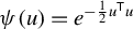 $\psi (u) = e^{-\frac {1}{2}u^{\mathsf {T}} u}$
. The first-order conditions are given by
 $$\begin{align*}u_j\left(\sum_{l = 1}^du_l\right) = r,\qquad j = 1,\ldots, d, \end{align*}$$
and we find that at the optimal solution
 $u_1 = \cdots = u_d = \sqrt {r/d}$
. Thus,
 $\left \lVert u\right \rVert _1 = \sqrt {rd}$
and
 $u^{\mathsf {T}} u = r$
, which completes the proof.
Lemma A.5. Suppose that
 $V = (Y,X) \in \mathbb {R}\times \mathbb {R}^d$
is a zero-mean random vector and that the moment conditions in Lemma A.2 hold. The functionals
 $\boldsymbol {b}_r(V)$
and
 $\boldsymbol {\zeta }_r(V)$
,
 $r \geq 1$
, are nonnegative and equal zero if and only if
 $\mathbb {E}(Y|X) = X^{\mathsf {T}}\theta ^*$
almost surely.
Proof. Lemma A.3 shows that
 $\theta = \theta ^*$
is necessary for boundedness of both
 $\boldsymbol {b}_r(V)$
and
 $\boldsymbol {\zeta }_r(V)$
,
 $r \geq 1$
. The next inequalities follow from Lemmas A.3 and A.4
 $$ \begin{align} \boldsymbol{\varsigma}(V)\leq C_r\boldsymbol{b}_r(V) \leq C_rA_\delta\boldsymbol{\zeta}_r(V), \end{align} $$
where
 $C_r$
and
 $A_\delta $
are positive constants.
Using the inequalities in equation (A.4) and Lemma A.1, we conclude that
 $\boldsymbol {\zeta }_r(V) = 0$
leads to
 $\mathbb {E}(Y|X) = X^{\mathsf {T}}\theta ^*$
almost surely. In the opposite direction, if
 $\mathbb {E}(Y|X) = X^{\mathsf {T}}\theta ^*$
almost surely, then
 $\mathbb {E}[(Y - X^{\mathsf {T}}\theta ^*)f(X)] = 0$
for any measurable function f for which the moment is defined and, therefore,
 $\boldsymbol {\zeta }_r(V) = 0$
. The same statements hold for
 $\boldsymbol {b}_r(V)$
.
Proof of Theorem 2
 $$ \begin{align*} \boldsymbol{\varsigma}(n^{-1/2}(\Delta V_{1} + \cdots + \Delta V_{n})) &\leq \boldsymbol{\varsigma}^{\theta^*}(n^{-1/2}(\Delta V_{1} + \cdots + \Delta V_{n}))\\ &\leq nC_{r}\boldsymbol{b}_{r}(n^{-1/2}V_{\Delta t})\\ & = n^{1 - \frac{r+1}{2}}C_{r}\boldsymbol{b}_{r}(V_{\Delta t}), \end{align*} $$
where
 $C_r = \sup _{u \in \mathbb {R}^d}\left \lVert u\right \rVert _1^{r}\psi (u)$
. The upper bound in equation (15) follows from Lemmas A.2 and A.3.
Lemma A.6. Suppose
 $Z = (Z_y,Z_x) \in \mathbb {R}\times \mathbb {R}^{d}$
is a strictly
 $\alpha $
-stable random vector with tail parameter
 $1 < \alpha \leq 2$
and a spectral measure
 $\Lambda $
. Denote by
 $\xi = (y,x)\in \mathbb {R}\times \mathbb {R}^{d}$
and let
 $\mathbb {S} = \{z\in \mathbb {R}^{d+1}\colon \left \lVert z\right \rVert _2 = 1\}$
be the unit sphere in
 $\mathbb {R}^{d+1}$
. If
 $\theta $
is a fixed vector of parameters, then the conditions
 $$ \begin{align*} &\int_{\mathbb{S}}(y - x^{\mathsf{T}}\theta)\,\mathrm{sign}(u^{\mathsf{T}} x)|u^{\mathsf{T}} x|^{\alpha - 1}\Lambda (d\xi) = 0,\quad \forall u \in \mathbb{R}^d\\ &\int_{\mathbb{S}}(y - x^{\mathsf{T}}\theta)|u^{\mathsf{T}} x|^{\alpha - 1}\Lambda(d\xi) = 0,\quad \forall u \in \mathbb{R}^d, \end{align*} $$
are identical with
 $\mathbb {E}[Z_y|Z_x] \overset {\scriptscriptstyle \mathit {a.s.}}{=} Z_x^{\mathsf {T}}\theta $
.
Proof. The plan is to calculate the expectation
 $\mathbb {E}(Z_y - Z_x^{\mathsf {T}}\theta )e^{iu^{\mathsf {T}} Z_x}$
and then show that the conditions in equations (24) and (25) are equivalent to requiring that the expectation vanishes for all
 $u \in \mathbb {R}^d$
.
Denote the ch.f. of
 $Z = (Z_y, Z_x)$
by
 $\varphi _Z(v,u) = \mathbb {E} e^{i(vZ_y + u^{\mathsf {T}} Z_x)}$
. The expectation can be expressed in terms of certain derivatives of the ch.f. and the vector of parameters
 $\theta $
 $$ \begin{align*} \mathbb{E}(Z_y - Z_x^{\mathsf{T}}\theta)e^{iu^{\mathsf{T}} Z_x} = \frac{\partial}{\partial v}\varphi_Z(0, u) - \sum_{k = 1}^d\theta_k\frac{\partial}{\partial u_{k}}\varphi_Z(0, u). \end{align*} $$
We express the right side as a function of the spectral measure using the explicit form of the ch.f. of stable laws (see Samorodnitsky and Taqqu, Reference Samorodnitsky and Taqqu1994, Chap. 2).
Adopt the notation
 $t = (v,u)$
. It is straightforward to calculate the derivative
 $$ \begin{align*} \frac{\partial}{\partial t_k}\varphi_Z(t) &= \frac{\partial}{\partial t_k}\exp\left\{-\int_{\mathbb{S}}|t^{\mathsf{T}} \xi|^{\alpha}\left(1 - i\,\mathrm{sign}(\xi^{\mathsf{T}} s)\tan\frac{\pi\alpha}{2}\right)\Lambda(d\xi)\right\}\\ &= \alpha\varphi_Z(t)\left(-\int_{\mathbb{S}}\xi_k\,\mathrm{sign}(t^{\mathsf{T}} \xi)|t^{\mathsf{T}} \xi|^{\alpha-1}\Lambda(d\xi) + i\int_{\mathbb{S}}\xi_k|t^{\mathsf{T}} \xi|^{\alpha-1}\tan\frac{\pi\alpha}{2}\Lambda(d\xi)\right). \end{align*} $$
Using this expression and
 $\varphi _Z(0, u) = \varphi _{Z_x}(u)$
, for the expectation, we obtain
 $$ \begin{align} \mathbb{E}(Z_y - Z_x^{\mathsf{T}}\theta)e^{iu^{\mathsf{T}} Z_x} &=\alpha\varphi_{Z_x}(u)\bigg(-\int_{\mathbb{S}}(y - x^{\mathsf{T}}\theta)\,\mathrm{sign}(u^{\mathsf{T}} x)|u^{\mathsf{T}} x|^{\alpha-1}\Lambda(d\xi) \nonumber\\ &\qquad + i\int_{\mathbb{S}}(y - x^{\mathsf{T}}\theta)|u^{\mathsf{T}} x|^{\alpha-1}\tan\frac{\pi\alpha}{2}\Lambda(d\xi)\bigg) \nonumber\\ &= -\alpha\varphi_{Z_x}(u)(\gamma(u) - i\eta(u)), \end{align} $$
where
 $\xi = (y, x)\in \mathbb {R}\times \mathbb {R}^d$
. As a result,
 $\mathbb {E}(Z_y - Z_x^{\mathsf {T}}\theta )e^{iu^{\mathsf {T}} Z_x} = 0$
for all
 $u \in \mathbb {R}^d$
if and only if
 $\gamma (u) = \eta (u) = 0$
for all
 $u \in \mathbb {R}^d$
because
 $\varphi _{Z_x}(u)$
is a complex exponential and does not vanish. The proof is now complete.
Lemma A.7. Denote by
 $V = (Y,X) \in \mathbb {R}\times \mathbb {R}^d$
and
 $Z = (Z_y,Z_x) \in \mathbb {R}\times \mathbb {R}^d$
two arbitrary random vectors and assume that for some
 $\theta ,$
the next conditions hold
 $$ \begin{align} \mathbb{E} \left[(Y - X^{\mathsf{T}}\theta)X^\nu - (Z_y - Z_x^{\mathsf{T}}\theta)Z_x^\nu\right] = 0,\quad \forall \nu\colon |\nu| \leq k. \end{align} $$
Define
 $$ \begin{align} \boldsymbol{\zeta}_r^\theta(V, Z) = \sup_{g\in\mathcal{G}}\left|\int_{\mathbb{R}^{d+1}}(y - x^{\mathsf{T}}\theta)g(x)d(F - G)\right|, \end{align} $$
where
 $\mathcal {G}$
is the class defined in equation (A.2). The following bound holds:
 $$ \begin{align*} \boldsymbol{\zeta}_{r}^\theta(V, Z) \leq \frac{\Gamma(\delta + 1)}{\Gamma(r + 1)}\int_{\mathbb{R}^{d+1}}|y - x^{\mathsf{T}}\theta|\left\lVert x\right\rVert_1^{r} \left|F - G\right|(d\xi), \end{align*} $$
where
 $\xi = (y ,x)$
,
 $r \geq 1$
,
 $r = k + \delta $
, where k is an integer,
 $\delta \in (0, 1]$
, and F and G are the distribution functions of V and Z, respectively.
Proof. The proof follows the same steps as that of Lemma A.2. The functions from the class
 $\mathcal {G}$
can be written in terms of their Taylor expansion at
 $x = 0$
 $$ \begin{align*} \begin{aligned} g(x) &= \sum_{|\nu| \leq k - 1}\frac{\partial^{\nu}g(0)}{\nu!}x^{\nu} + {k}\sum_{|\nu| = k}\frac{x^{\nu}}{\nu!}\int_{0}^{1}(1 - u)^{k-1}\partial^{\nu}g(ux)du. \end{aligned} \end{align*} $$
To simplify the notation, denote the two residuals by
 $\varepsilon = Y - X^{\mathsf {T}}\theta $
and
 $\eta = Z_y - Z_x^{\mathsf {T}}\theta $
. For the expectation in the definition of
 $\boldsymbol {\zeta }_r$
, we can write
 $$ \begin{align*} I &= \mathbb{E}\left(\varepsilon g(X) - \eta g(Z_x)\right) \\&= \sum_{|\nu| \leq k - 1}\frac{\partial^{\nu}g(0)}{\nu!}\mathbb{E} \left[\varepsilon X^\nu - \eta Z_x^\nu\right] \\ &\quad + k\sum_{ |\nu| = k}\int_{0}^{1}\frac{(1 - u)^{ k-1}}{\nu!}\mathbb{E}\left(\varepsilon X^{\nu}\partial^{\nu}g(uX) - \eta Z_x^{\nu}\partial^{\nu}g(uZ_x)\right)du. \end{align*} $$
The first sum vanishes due to the condition in equation (A.6). The expectations in the integral can be written in the following way:
 $$\begin{align*}\mathbb{E}\left(\varepsilon X^{\nu}\partial^{\nu}g(uX) - \eta Z_x^{\nu}\partial^{\nu}g(uZ_x)\right) = \int_{\mathbb{R}^{d+1}}(y - x^{\mathsf{T}}\theta)x^\nu \left[\partial^\nu g(ux) - \partial^\nu g(0)\right]d(F-G), \end{align*}$$
in which F and G are the distribution functions of V and Z and
 $$\begin{align*}\partial^\nu g(0)\int_{\mathbb{R}^{d+1}}(y - x^{\mathsf{T}}\theta) x^\nu d(F-G) = \partial^\nu g(0)\mathbb{E} \left(\varepsilon X^\nu - \eta Z_x^\nu\right) = 0 \end{align*}$$
follows from equation (A.6) with
 $|\nu | = k$
. As a result, we obtain
 $$\begin{align*}I = k\sum_{|\nu| = k}\int_{0}^{1}\frac{(1 - u)^{k-1}}{\nu!}\left[\int_{\mathbb{R}^{d+1}}(y - x^{\mathsf{T}}\theta )x^\nu \left(\partial^\nu g(ux) - \partial^\nu g(0)\right)d(F-G)\right]du. \end{align*}$$
The absolute value
 $|I|$
is bounded in the same way as in the proof of Lemma A.2. As a result, for any
 $g\in \mathcal {G,}$
we obtain
 $$\begin{align*}\left|\mathbb{E} \varepsilon g(X) - \mathbb{E}\eta g(Z_x)\right| = |I| \leq \frac{\Gamma(\delta + 1)}{\Gamma(r + 1)}\int_{\mathbb{R}^{d+1}}|y - x^{\mathsf{T}}\theta|\left\lVert x\right\rVert_1^{k+\delta} \left|F-G\right|(d\xi), \end{align*}$$
where
 $\xi = (y, x)$
and the proof is completed after taking the supremum over all
 $g \in \mathcal {G}$
.
Lemma A.8. Denote by
 $V = (Y,X) \in \mathbb {R}\times \mathbb {R}^d$
and
 $Z = (Z_y,Z_x) \in \mathbb {R}\times \mathbb {R}^d$
two arbitrary random vectors. The following inequality holds:
 $$ \begin{align*} \boldsymbol{b}_r^\theta(V, Z) \leq A_\delta\boldsymbol{\zeta}_r^\theta(V, Z), \end{align*} $$
where
 $r \geq 1$
,
 $r = k + \delta $
, in which k is an integer,
 $\delta \in (0, 1]$
, and
 $\theta $
is fixed. The next scaling property holds
 $$ \begin{align*} \boldsymbol{b}_r^\theta(aV, aZ) = |a|^{r+1}\boldsymbol{b}_r^\theta(V, Z), \end{align*} $$
where
 $a\in \mathbb {R}$
is a constant.
Proof. The proof is the same as that of Lemma A.3 and relies on the properties of the functional
 $\boldsymbol {\zeta }_r^\theta (V,Z)$
defined in equation (A.7), which are established in Lemma A.7.
Lemma A.9. Suppose
 $Z_j = (Z_{y,j}, Z_{x,j}) \in \mathbb {R}\times \mathbb {R}^d$
are independent copies of a strictly
 $\alpha $
-stable random vector
 $Z = (Z_y, Z_x)$
with
 $1 < \alpha \leq 2$
. Then,
 $$ \begin{align*} \mathbb{E}\left(\frac{1}{n^{1/\alpha}}\sum_{j = 1}^n\left(Z_{y,j} - Z_{x,j}^{\mathsf{T}} \theta\right)e^{iu^{\mathsf{T}}\frac{Z_{x,j}}{n^{1/\alpha}}}\right) = -\alpha\varphi_{Z_x}(n^{-1/\alpha}u) \omega_{\alpha,\Lambda}(u), \end{align*} $$
where
 $\varphi _{Z_x}(u) = \mathbb {E} e^{iu^{\mathsf {T}} Z_x}$
is the ch.f. of
 $Z_x$
,
 $$ \begin{align*} \omega_{\alpha,\Lambda}(u) = \int_{\mathbb{S}}(y - x^{\mathsf{T}}\theta)(u^{\mathsf{T}} x)^{\alpha-1}\Lambda(d\xi) - i\int_{\mathbb{S}}(y - x^{\mathsf{T}}\theta)|u^{\mathsf{T}} x|^{\alpha-1}\tan\frac{\pi\alpha}{2}\Lambda(d\xi), \end{align*} $$
in which
 $\xi = (y,x)\in \mathbb {R}\times \mathbb {R}^d$
,
 $(x)^\alpha = \,\mathrm {sign}(x)|x|^\alpha $
, and
 $\Lambda $
is the spectral measure of Z.
Proof. Using independence, it is easy to see that
 $$ \begin{align*} \mathbb{E}\left(\frac{1}{n^{1/\alpha}}\sum_{j = 1}^n\left(Z_{y,j} - Z_{x,j}^{\mathsf{T}} \theta\right)e^{iu^{\mathsf{T}}\frac{Z_{x,j}}{n^{1/\alpha}}}\right) = n^{\frac{\alpha - 1}{\alpha}}\mathbb{E}(Z_y - Z_x^{\mathsf{T}}\theta)e^{iu^{\mathsf{T}}\frac{Z_x}{n^{1/\alpha}}}. \end{align*} $$
The expectation on the right side is treated similarly as in the proof of Lemma A.6. Using equation (A.5), we obtain
 $$ \begin{align*} n^{\frac{\alpha - 1}{\alpha}}\mathbb{E}(Z_y - Z_x^{\mathsf{T}}\theta)e^{iu^{\mathsf{T}}\frac{Z_x}{n^{1/\alpha}}} &= -n^{\frac{\alpha - 1}{\alpha}}\alpha\varphi_{Z_x}\left(\frac{u}{n^{1/\alpha}}\right)\left[\gamma\left(\frac{u}{n^{1/\alpha}}\right) - i\eta\left(\frac{u}{n^{1/\alpha}}\right)\right]\\ &= -\alpha\varphi_{Z_x}\left(\frac{u}{n^{1/\alpha}}\right)(\gamma(u) - i\eta(u)), \end{align*} $$
which completes the proof.
Proof of Theorem 3
To simplify the expressions in the proof, we modify the notation in the following way. The two Lévy processes are denoted by
 $V(t) = (Y(t), X(t))$
and
 $Z(t) = (Z_y(t), Z_x(t))$
. We construct n intervals of equal fixed length
 $t_{i} - t_{i-1} = \Delta t$
, where
 $t_0 = 0$
and
 $i = 1, \ldots , n$
. From the definition of Lévy processes,
 $$\begin{align*}V(n\Delta t) = \sum_{i = 1}^n\Delta V(t_{i} - t_{i-1}) = \sum_{i = 1}^nV_i, \end{align*}$$
in which
 $V_1, \ldots , V_n$
are independent copies of a random vector
 $V_0$
with a distribution function F because the increments in the sum are considered over intervals of the same length. The notation for the process
 $Z(t)$
is analogous; that is,
 $Z_1, \ldots , Z_n$
is a sequence of independent copies of a random vector
 $Z_0$
with a distribution function G representing increments over intervals of the same length
 $\Delta t$
.
By assumption, the vector
 $Z_{0}$
has a strictly
 $\alpha $
-stable distribution and satisfies the stability property
 $Z_{0} \overset {\scriptscriptstyle d}{=} n^{-1/\alpha }\sum _{i = 1}^n Z_{i}$
. The stability property implies that
 $\mathbb {E} [g(Z_0)] = \mathbb {E} [g(n^{-1/\alpha }\sum _{i = 1}^nZ_i)$
], where g is a measurable function and the moment is assumed to exist.
Using Assumption 1†
, there exists
 $\theta _\alpha ^*$
which satisfies equations (24) and (25) and we set
 $\theta = \theta _\alpha ^*$
everywhere in the proof. With that choice of
 $\theta $
, by Theorem 1 and Lemma A.6, the conditional mean of
 $Z_0$
is linear and
 $\mathbb {E}(Z_{y,0} - Z_{x,0}^{\mathsf {T}}\theta )e^{iu^{\mathsf {T}} Z_{x,0}} = 0$
for all u. Consider the following difference:
 $$ \begin{align*} \Delta_n &{:=}q \mathbb{E}\left(\frac{1}{n^{1/\alpha}}\left(Y(n\Delta t) - X(n\Delta t)^{\mathsf{T}}\theta\right)e^{iu^{\mathsf{T}} \frac{1}{n^{1/\alpha}}X(n\Delta t)}\right) - \mathbb{E}(Z_{y,0} - Z_{x,0}^{\mathsf{T}}\theta)e^{iu^{\mathsf{T}} Z_{x,0}}\\ &= \mathbb{E}\left(\frac{1}{n^{1/\alpha}}\sum_{j = 1}^n(Y_j - X_j^{\mathsf{T}}\theta)e^{iu^{\mathsf{T}} \frac{1}{n^{1/\alpha}}\sum_{k = 1}^nX_k}\right) \\ &\quad- \mathbb{E}\left(\frac{1}{n^{1/\alpha}}\sum_{j = 1}^n(Z_{y,j} - Z_{x,j}^{\mathsf{T}}\theta)e^{iu^{\mathsf{T}} \frac{1}{n^{1/\alpha}}\sum_{k = 1}^nZ_{x,k}}\right), \end{align*} $$
where we also applied the stability property. In each summand, we isolate the j-th term in the sum in the exponent and use the independence property
 $$ \begin{align*} \Delta_n &= \mathbb{E}\left(\frac{1}{n^{1/\alpha}}\sum_{j = 1}^n(Y_j - X_j^{\mathsf{T}}\theta)e^{iu^{\mathsf{T}} \frac{1}{n^{1/\alpha}}X_j}\right)\mathbb{E} e^{iu^{\mathsf{T}} \frac{1}{n^{1/\alpha}}\sum_{k \not = j}X_k} \\ &\quad- \mathbb{E}\left(\frac{1}{n^{1/\alpha}}\sum_{j = 1}^n(Z_{y,j} - Z_{x,j}^{\mathsf{T}}\theta)e^{iu^{\mathsf{T}} \frac{1}{n^{1/\alpha}}Z_{x,j}}\right)\mathbb{E} e^{iu^{\mathsf{T}} \frac{1}{n^{1/\alpha}}\sum_{k \not = j}Z_{x,k}}\\ &= I_n\mathbb{E} e^{iu^{\mathsf{T}} \frac{1}{n^{1/\alpha}}\sum_{k \not = j}X_k} - J_n\mathbb{E} e^{iu^{\mathsf{T}} \frac{1}{n^{1/\alpha}}\sum_{k \not = j}Z_{x,k}}. \end{align*} $$
Next, we add and subtract
 $J_n$
to the term
 $I_n$
 $$ \begin{align*} \Delta_n &= (I_n - J_n)\mathbb{E} e^{iu^{\mathsf{T}} \frac{1}{n^{1/\alpha}}\sum_{k \not = j}X_k} - J_n\left(\mathbb{E} e^{iu^{\mathsf{T}} \frac{1}{n^{1/\alpha}}\sum_{k \not = j}Z_{x,k}} - \mathbb{E} e^{iu^{\mathsf{T}} \frac{1}{n^{1/\alpha}}\sum_{k \not = j}X_k}\right). \end{align*} $$
The second term is related to the distance between the ch.f. of the normalized sums, while the first term is handled separately. The absolute value of the left side is bounded by
 $$ \begin{align*} |\Delta_n| \leq |I_n - J_n|\left|\mathbb{E} e^{iu^{\mathsf{T}} \frac{1}{n^{1/\alpha}}\sum_{k \not = j}X_k}\right| + |J_n|\left|\mathbb{E} e^{iu^{\mathsf{T}} \frac{1}{n^{1/\alpha}}\sum_{k \not = j}Z_{x,k}} - \mathbb{E} e^{iu^{\mathsf{T}} \frac{1}{n^{1/\alpha}}\sum_{k \not = j}X_k}\right|. \end{align*} $$
Next, multiply both sides by
 $\psi (u)$
,
 $$ \begin{align} \nonumber \psi(u)|\Delta_n| &\leq \psi(u)|I_n - J_n|\left|\mathbb{E} e^{iu^{\mathsf{T}} \frac{1}{n^{1/\alpha}}\sum_{k \not = j}X_k}\right| \\ &\quad + \psi(u)|J_n|\left|\mathbb{E} e^{iu^{\mathsf{T}} \frac{1}{n^{1/\alpha}}\sum_{k \not = j}^nZ_{x,k}} - \mathbb{E} e^{iu^{\mathsf{T}} \frac{1}{n^{1/\alpha}}\sum_{k \not = j}X_k}\right| \end{align} $$
 $$ \begin{align}\hphantom{\psi(u)|\Delta_n|} &= \psi(u)\left\lVert u\right\rVert_1^{r}\left\lVert u\right\rVert_1^{-r}|I_n - J_n|\left|\mathbb{E} e^{iu^{\mathsf{T}} \frac{1}{n^{1/\alpha}}\sum_{k \not = j}X_k}\right| \nonumber\\ &\quad + \psi(u)\left\lVert u\right\rVert_1^{\alpha-1}\left\lVert u\right\rVert_1^{1-\alpha}|J_n| \nonumber\\ &\quad \times\left|\mathbb{E} e^{iu^{\mathsf{T}} \frac{1}{n^{1/\alpha}}\sum_{k \not = j}Z_{x,k}} - \mathbb{E} e^{iu^{\mathsf{T}} \frac{1}{n^{1/\alpha}}\sum_{k \not = j}X_k}\right|\nonumber\\ &\leq C_r\sup_u\left\lVert u\right\rVert_1^{-r}|I_n - J_n| + 2C_{\alpha -1}\left(\sup_u\left\lVert u\right\rVert_1^{1-\alpha}|J_n|\right), \end{align} $$
where
 $C_p = \sup _u\left \lVert u\right \rVert _1^{p}\psi (u)$
and we used the inequality
 $|e^{ix}| \leq 1$
.
It remains to show the rate of decay of the right side of (A.9). We begin with the last term. From the result in Lemma A.9, we obtain
 $$ \begin{align*} \left\lVert u\right\rVert_1^{1-\alpha}|J_n| &\leq \alpha\left\lVert u\right\rVert_1^{1-\alpha} |\omega_{\alpha,\Lambda}(u)|, \end{align*} $$
in which
 $\Lambda $
denotes the spectral measure. From Assumption 1†
,
 $\theta $
satisfies equations (24) and (25). The two equations guarantee
 $|\omega _{\alpha ,\Lambda }(u)| = 0$
and, as a consequence, the second term in equation (A.9) vanishes.
The first term in (A.9) contains the expression
 $I_n - J_n$
which we represent in the following manner:
 $$ \begin{align*} I_n - J_n &= \mathbb{E}\left(\frac{1}{n^{1/\alpha}}\sum_{j = 1}^n(Y_j - X_j^{\mathsf{T}}\theta)e^{iu^{\mathsf{T}} \frac{1}{n^{1/\alpha}}X_j}\right) - \mathbb{E}\left(\frac{1}{n^{1/\alpha}}\sum_{j = 1}^n(Z_{y_j} - Z_{x,j}^{\mathsf{T}}\theta)e^{iu^{\mathsf{T}} \frac{1}{n^{1/\alpha}}Z_{x,j}}\right) \\ &= \frac{1}{n^{1/\alpha}}\sum_{j = 1}^n\left(\mathbb{E}(Y_j - X_j^{\mathsf{T}}\theta)e^{iu^{\mathsf{T}} \frac{1}{n^{1/\alpha}}X_j} - \mathbb{E}(Z_{y_j} - Z_{x,j}^{\mathsf{T}}\theta)e^{iu^{\mathsf{T}} \frac{1}{n^{1/\alpha}}Z_{x,j}}\right)\\ &= n^{1-\frac{1}{\alpha}}\left(\mathbb{E}(Y_0 - X_0^{\mathsf{T}}\theta)e^{iu^{\mathsf{T}} \frac{1}{n^{1/\alpha}}X_0} - \mathbb{E}(Z_{y,0} - Z_{x,0}^{\mathsf{T}}\theta)e^{iu^{\mathsf{T}} \frac{1}{n^{1/\alpha}}Z_{x,0}}\right)\\ &= n^{1-\frac{1}{\alpha}}\int_{\mathbb{R}^{d+1}}(y - x^{\mathsf{T}}\theta)e^{iu^{\mathsf{T}} \frac{1}{n^{1/\alpha}}x}d(F - G). \end{align*} $$
Thus, for the first term in (A.9), we obtain
 $$ \begin{align*} \left\lVert u\right\rVert_1^{-r}|I_n - J_n| &= n^{1 - \frac{1}{\alpha}}\left\lVert u\right\rVert_1^{-r}\left|\int_{\mathbb{R}^{d+1}}(y - x^{\mathsf{T}}\theta)e^{iu^{\mathsf{T}} \frac{1}{n^{1/\alpha}}x}d(F - G)\right|\\ &= n^{1 - \frac{r+1}{\alpha}}\left\lVert v\right\rVert_1^{-r}\left|\int_{\mathbb{R}^{d+1}}(y - x^{\mathsf{T}}\theta)e^{iv^{\mathsf{T}} x}d(F - G)\right|, \end{align*} $$
where
 $v = u/n^{1/\alpha }$
. As a result,
 $$ \begin{align} \sup_u\left\lVert u\right\rVert_1^{-r}|I_n - J_n| &= n^{1 - \frac{r+1}{\alpha}}\sup_v\left\lVert v\right\rVert_1^{-r}\left|\int_{\mathbb{R}^{d+1}}(y - x^{\mathsf{T}}\theta)e^{iv^{\mathsf{T}} x}d(F - G)\right|\nonumber\\ &= n^{1 - \frac{r+1}{\alpha}}\boldsymbol{b}_r^\theta(V_0, Z_0). \end{align} $$
We need to provide conditions under which the right side in the equation above is finite. Applying Lemmas A.7 and A.8, we obtain
 $$ \begin{align*} \boldsymbol{b}_r^\theta(V_0, Z_0) \leq A_\delta\frac{\Gamma(\delta + 1)}{\Gamma(r + 1)}\int_{\mathbb{R}^{d+1}}|y - x^{\mathsf{T}}\theta|\left\lVert x\right\rVert_1^r|F - G|(d(y,x)), \end{align*} $$
where
 $r = k + \delta $
,
 $k \geq 1$
is an integer and
 $\delta \in (0,1]$
.
The final form of the upper bound in (35) is obtained by plugging the expressions in equation (A.10) into (A.9)
 $$\begin{align*}\psi(u)|\Delta_n| \leq C_rn^{1 - \frac{r+1}{\alpha}}\boldsymbol{b}_r^\theta(V_0, Z_0). \end{align*}$$
Proof of Theorem 4
The proof uses the notation adopted in the proof of Theorem 3. Starting from the expression for
 $\psi (u)|\Delta _n|$
provided in equation (A.8), we obtain
 $$ \begin{align} \psi(u)|\Delta_n| &\leq \psi(u)|I_n - J_n|\left|\mathbb{E} e^{iu^{\mathsf{T}} \frac{1}{n^{1/\alpha}}\sum_{k \not = j}X_k}\right| \nonumber\\&\quad + \psi(u)|J_n|\left|\mathbb{E} e^{iu^{\mathsf{T}} \frac{1}{n^{1/\alpha}}\sum_{k \not = j}^nZ_{x,k}} - \mathbb{E} e^{iu^{\mathsf{T}} \frac{1}{n^{1/\alpha}}\sum_{k \not = j}X_k}\right| \nonumber\\&= \psi(u)\left\lVert u\right\rVert_1^{r}\left\lVert u\right\rVert_1^{-r}|I_n - J_n|\left|\mathbb{E} e^{iu^{\mathsf{T}} \frac{1}{n^{1/\alpha}}\sum_{k \not = j}X_k}\right| \nonumber\\&\quad + \psi(u)\left\lVert u\right\rVert_1^{s+\alpha-1}\left\lVert u\right\rVert_1^{1-\alpha}|J_n| \nonumber\\&\quad \times\left\lVert u\right\rVert_1^{-s}\left|\mathbb{E} e^{iu^{\mathsf{T}} \frac{1}{n^{1/\alpha}}\sum_{k \not = j}Z_{x,k}} - \mathbb{E} e^{iu^{\mathsf{T}} \frac{1}{n^{1/\alpha}}\sum_{k \not = j}X_k}\right|\nonumber\\&\leq C_r\sup_u\left\lVert u\right\rVert_1^{-r}|I_n - J_n| \nonumber\\&\quad + C_{s+\alpha -1}\left(\sup_u\left\lVert u\right\rVert_1^{1-\alpha}|J_n|\right){\boldsymbol{\chi}}_s\left(\frac{1}{n^{1/\alpha}}\sum_{k = 1}^{n-1}X_k,\frac{1}{n^{1/\alpha}}\sum_{k = 1}^{n-1}Z_{x,k}\right), \end{align} $$
where
 $C_p = \sup _u\left \lVert u\right \rVert _1^{p}\psi (u)$
and
 ${\boldsymbol {\chi }}_s$
is defined in equation (32).
It remains to show the rate of decay of the right side of (A.11). From the result in Lemma A.9, we obtain
 $$ \begin{align} \left\lVert u\right\rVert_1^{1-\alpha}|J_n| \leq \alpha\left\lVert u\right\rVert_1^{1-\alpha} |\omega_{\alpha,\Lambda}(u)| &= \alpha \left|\omega_{\alpha,\Lambda}\left(\frac{u}{\left\lVert u\right\rVert_1}\right)\right| \nonumber\\ &\leq \alpha \sup_{v\in B}|\omega_{\alpha,\Lambda}(v)||\nonumber\\ &= \alpha D_{\alpha}, \end{align} $$
in which
 $B = \{z\in \mathbb {R}^d\colon \left \lVert z\right \rVert _1 = 1\}$
and
 $\Lambda $
denotes the spectral measure. For the first term in (A.11), we use the expression derived in equation (A.10). The final form of the upper bound in (35) is obtained by plugging in the expressions in equations (A.12) and (A.10) into (A.11). From the ideality properties of the
 ${\boldsymbol {\chi }}_s$
metric (Rachev et al., Reference Rachev, Klebanov, Stoyanov and Fabozzi2013, Chap. 15),
 $$ \begin{align*} {\boldsymbol{\chi}}_s\left(\frac{1}{n^{1/\alpha}}\sum_{k = 1}^{n-1}X_k,\frac{1}{n^{1/\alpha}}\sum_{k = 1}^{n-1}Z_{x,k}\right) &\leq (n-1)n^{-s/\alpha}{\boldsymbol{\chi}}_s(X_0, Z_{x,0}) \\ &\leq n^{1-s/\alpha}{\boldsymbol{\chi}}_s(X_0, Z_{x,0}), \end{align*} $$
which completes the proof.
The conditions in equation (33) guarantee boundedness of
 ${\boldsymbol {\chi }}_s$
. We now demonstrate that they also guarantee boundedness of
 $\boldsymbol {b}_{s-1}$
. If we represent
 $\xi = (y, x_1, \ldots , x_d) $
, then from the first condition in (33), we obtain
 $$\begin{align*}\int_{\mathbb{R}^{d+1}}yx^\nu d(F-G) = 0 \quad \text{and}\quad \int_{\mathbb{R}^{d+1}}x_jx^\nu d(F-G) = 0,\quad \forall \nu\colon |\nu| \leq k -1, \end{align*}$$
where
 $j = 1,\ldots ,d$
. Then, any linear combination of these integrals equals zero and, thus, the condition in equation (A.6) holds for all multi-indices
 $\nu $
such that
 $|\nu | \leq k -1$
. The absolute pseudomoment
 ${\boldsymbol {v}}_s(V_0, Z_0)$
is assumed bounded in (33). Combining this with the inequality in equation (29) and Lemma A.8 shows that
 $\boldsymbol {b}_{s-1}$
is bounded as well.
Proof of Theorem 5
Assumption 1‡
ensures that the least-squares estimator for the vector
 $\sum _{l = 1}^nV_l$
is
 $\theta ^*$
provided in Assumption 2‡
. Repeating the steps in Lemma A.4 while bearing in mind
 $V_1, V_2, \dots $
are non-identically distributed yields
 $$ \begin{align*} \boldsymbol{\zeta}^{\theta^*}\left(\sum_{l = 1}^nV_l\right) &= \sup_{u}\psi(u)\left|\mathbb{E}\left(\sum_{l=1}^n\left(Y_l - X_l^{\mathsf{T}}\theta^*\right)\right)e^{i u^{\mathsf{T}} \left(\sum_{m=1}^{n}X_m\right)}\right| \\ & \leq \sum_{l=1}^n\sup_{u}\psi(u)\left|\mathbb{E}\left(Y_l - X_l^{\mathsf{T}}\theta^*\right)e^{iu^{\mathsf{T}} X_l}\right|\\ &\leq \left(\sup_{u}\psi(u)\left\lVert u\right\rVert^{r}_1\right)\sum_{l=1}^n\sup_{u}\left\lVert u\right\rVert_1^{-r}\left|\mathbb{E}\left(Y_l - X_l^{\mathsf{T}}\theta^*\right)e^{iu^{\mathsf{T}} X_l}\right|\\ &= C_r\sum_{l = 1}^n\boldsymbol{b}_r(V_l). \end{align*} $$
Assumption 2‡
ensures that the quantities
 $\boldsymbol {b}_r(V_l)$
are finite. Combining this estimate with Lemma A.3, we obtain
 $$\begin{align*}\boldsymbol{\zeta}\left(n^{-1/2}\sum_{l = 1}^nV_l\right) \leq \boldsymbol{\zeta}^{\theta^*}\left(n^{-1/2}\sum_{l = 1}^nV_l\right) \leq C_r n^{-\frac{r+1}{2}}\sum_{l = 1}^n\boldsymbol{b}_r(V_l). \end{align*}$$
Applying Lemmas A.2 and A.3 to each term
 $\boldsymbol {b}_r(V_l)$
leads to an upper bound analogous to the one in equation (15). Summing up all terms and applying the inequality in equation (51) from Assumption 2‡
yields,
 $$\begin{align*}\sum_{l = 1}^n\boldsymbol{b}_{r}(V_{l}) \leq A_\delta \frac{\Gamma(\delta + 1)}{\Gamma(r + 1)}\sum_{l = 1}^n\mathbb{E}\left(|Y_{l} - X_{l}^{\mathsf{T}}\theta^*|\left\lVert X_{l}\right\rVert_1^{r}\right) \leq nA_\delta \frac{\Gamma(\delta + 1)}{\Gamma(r + 1)}D, \end{align*}$$
which completes the proof.
FUNDING STATEMENT
The author declares that no specific funding has been received for this article.
COMPETING INTEREST STATEMENT
The author declares that no competing interests exist.