I. INTRODUCTION
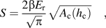
The Oliver–Pharr methodReference Oliver and Pharr1, Reference Oliver and Pharr2 provides a way to evaluate load–displacement data obtained by instrumented indentation, based on Sneddon’sReference Sneddon3 elastic contact theory. It is mainly based on two equations, the first of which relates the contact stiffness S to the contact area A c:
whereas the second provides an expression for the contact depth h c by predicting the magnitude of the elastic sink-in around the indenter:
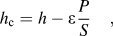
where ε is a geometrical constant that depends on the shape of the indenter. For a cone with an opening angle equivalent to the Berkovich indenter, a value of ε = 0.72 was calculated.Reference Oliver and Pharr1 However, Oliver and PharrReference Oliver and Pharr1 pointed out that plastic deformation modifies the contact shape from an early stage of the indentation onwards. They observed from load–displacement curves that most of the time the unloading segment rather corresponds to what is expected from a purely elastic deformation by an indenter with the shape of a paraboloid of revolution. Consequently, they retained a value of ε = 0.75.
Later, Bolshakov et al.Reference Bolshakov, Oliver, Pharr, Baker, Ross, Townsend, Volkert and Børgesen4 and Pharr and BolshakovReference Pharr and Bolshakov5 introduced the concept of the effective indenter to provide a general explanation for the discrepancy between the indenter geometry and the shape of the resulting unloading curve. More precisely, Pharr and BolshakovReference Pharr and Bolshakov5 demonstrated that the elastic contact of a real indenter with a residual indent is equivalent to the elastic contact of a so-called “effective indenter” with a flat surface. They assumed that the shape of the effective indenter can be described by a power-law relation:

and that the unloading segment of the real indentation curve can be fitted by the power-law function:

where A, h f, and m are the coefficients to be determined by fitting. They showed that those values fully characterize the effective indenter, owing to the relations:

and
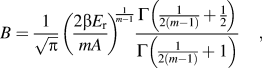
where Γ is the gamma function and E r is the reduced indentation modulus of the material. This model was validated by finite element simulations for elastic-plastic materials. In the work of Pharr and Bolshakov,Reference Pharr and Bolshakov5 Eq. (6) is expressed with the constant β set to one. Since this is not widely accepted yet, we prefer to use here the more general formulation with the β factor. The effective indenter shape strongly depends on the tested material and on the geometry of the used indenter. Based on the effective indenter analysis, ε can be more accurately calculated asReference Pharr and Bolshakov5, Reference Woirgard and Dargenton6:
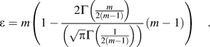
SchwarzerReference Schwarzer7 extended the scope of the effective indenter concept to the determination of the stress field under the indenter. Such an analysis was subsequently successfully applied to different systems.Reference Schwarzer8, Reference Herrmann and Richter9
II. THE EFFECTIVE INDENTER SHAPE REVEALED BY THE STIFFNESS DATA
The calibration procedure of the Oliver and PharrReference Oliver and Pharr1, Reference Oliver and Pharr2 method aims at determining the tip area function, which amounts to measuring the geometry of the indenter. For a known material, Eq. (1) provides from the current contact stiffness the size of the corresponding contact area, while Eq. (2) is used simultaneously to measure the contact depth. Once the relation between the indenter height and its cross-sectional area is known, it is possible, given a few theoretical assumptions, to reconstruct the geometry of the indenter. A commonly made approximation is the symmetry of revolution around the vertical axis of the indenter, which makes it sufficient to calculate the so-called contact radius a c. Equation (1) can thus be rewritten as:
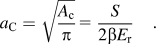
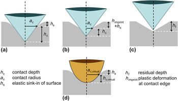
As illustrated in Fig. 1(a), the knowledge of the variation of a c and h c during the loading sequence allows a full reconstruction of the geometry of the tip.
Schematic of the indenter (a) at maximum load (b) during unloading, (c) after unloading, and (d) corresponding effective indenter. The deformations are exaggerated. The sink-in of the surface around the indenter is noted as h s= ε · P/S.

With the approximation proposed above, a three-sided pyramidal indenter would be represented by an equivalent cone with a somehow larger included angle. This equivalence might seem questionable at first but has nonetheless been successfully used in many simulations to predict the behavior of real pyramidal indenters.Reference Larsson, Giannakopoulos, Söderlund, Rowcliffe and Vestergaard10–Reference Backes, Durst and Göken13 The indenter shape reconstruction based on Eqs. (2) and (8) is especially meaningful for dynamic nanoindentation where the stiffness is continuously recorded during indentation.Reference Hay, Agee and Herbert14
In this study, this well-known procedure has been extended to derive the shape of the effective indenter. This is achieved by measuring the stiffness during the unloading of the indenter.
First, it is important to understand how the inherent differences between loading and unloading can affect the validity of the Oliver–Pharr equations. Pharr et al.Reference Pharr, Oliver and Brotzen15 have shown that Eqs. (1) and (8) are valid for all kinds of axisymmetric indenters so this remains in particular true during the unloading sequence. However, Eq. (2) no longer predicts the contact depth of the indenter. Indeed, during the course of the removal of the tip, the residual impression forms gradually at the outskirt of the contact, leading to the geometrical consequences shown in Fig. 1(b).
Consequently, Eq. (2) has to be modified for the unloading sequence into:
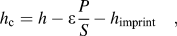
where h imprint varies from 0 at the beginning of the unloading process to h f at its end. It will be shown later what h imprint represents and how it can be measured. For the moment, it is sufficient to be aware that the real indenter does not follow the original Oliver–Pharr equations throughout the unloading process. However, even more importantly, the virtual effective indenter does, because of its definition.
As already mentioned in the introduction, the effective indenter is a punch of unknown shape acting elastically on a flat surface located at a different height than the original real surface. The difference between both heights corresponds to the residual plastic deformation at the center of the indent, i.e., h f, which can be obtained from the load–displacement data. The application of Eqs. (2) and (8) of the Oliver–Pharr method to this newly defined system directly reveals the shape of the effective indenter, as illustrated by Fig. 1(d).
More precisely, Eq. (8) is kept as:
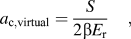
while Eq. (2) should now be expressed as:
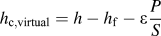
because of the new surface definition.
The present work was done within the framework of Sneddon’s theory.Reference Sneddon3 Since it has been revealed recently that his analytical solution does not take into consideration the radial displacements of the surface under the indenter,Reference Hay, Bolshakov and Pharr16 there is a risk of slightly overestimating the area of the residual imprint. This issue is, however, general and can be solved by selecting an appropriate valueReference Oliver and Pharr2 for β, possibly obtained from a corrective model.Reference Hay, Bolshakov and Pharr16, Reference Chudoba and Jennett17
III. EXPERIMENTAL
Nanoindentation measurements were performed with a Nanoindenter G200 (Agilent Technologies, Oak Ridge, TN) system equipped with a diamond Berkovich pyramid mounted into the standard XP measurement head. A new method was developed, which operated the device with the continuous stiffness measurement (CSM) module turned on until the very end of the unloading sequence. Moreover, the corrections suggested by Pharr et al.Reference Pharr, Strader and Oliver18 to minimize the effects of the dynamic unloading were applied. Typically, the CSM system was set to oscillate the tip at 69 Hz with 3-nm harmonic amplitude. The unloading was performed at a decreasing unloading rate, with the indentation strain rate  being held constant. This ensured a more reliable recording of the last part of the unloading, during which an increasingly fast change of the contact area occurs. Whenever achievable, indentation was performed with a maximal displacement into surface of 2000 nm. The loading sequence was followed by a 30-s holding segment, and unloading was finally performed according to the above description until 98% of the load was removed. For the determination of ε in fused silica, a series of 16 indentations were performed with nine partial unloading steps of 30% so that the value of ε could be calculated at different depths.
The materials used in this study were fused silica, sapphire, nanocrystalline nickel (nc-Ni), and ultrafine-grained aluminum (ufg-Al) samples. Fused silica and sapphire are the most commonly used reference materials because they exhibit a large elastic recovery and no pileup. The nc-Ni was produced by pulsed electrodeposition,Reference Natter and Hempelmann19–Reference Maier, Durst, Mueller, Backes, Höppel and Göken22 whereas the ufg-Al samples were obtained by means of accumulative roll-bondingReference Höppel, May and Göken23, Reference Böhner, Maier, Durst, Höppel and Göken24 of commercially pure aluminum (AA1050A). Because of the extremely small grain size, both materials can be considered to behave isotropically since the indentation depth of 2000 nm is much larger than the grain size. This is of great importance for the use of the contact stiffness for calculating contact radii.
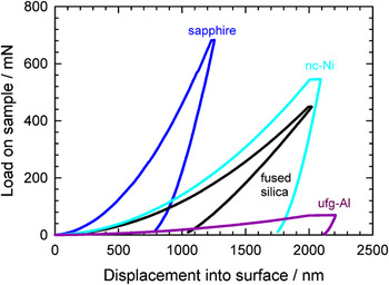
These different materials have been chosen to cover a broad range of mechanical properties, which is clearly visible from the load–displacement curves in Fig. 2. From the slopes of the unloading segments, it is obvious that a much larger part of the deformation is stored elastically in fused silica than in any other material. Lastly, it should be pointed out that only nc-Ni and ufg-Al experience significant creep during the 30-s hold segment.
Load–displacement curves of the tested materials.

The reduced elastic moduli E r needed for the calculations of the effective indenter shape were directly determined from the nanoindentation data of each material, following the standard Oliver–Pharr method, and are reported in Table I. As no supplementary pileup correction was applied, a slight underestimation of the contact area and overestimation of the elastic modulus cannot be ruled out, especially for the metals. This is, however, a general issue with the Oliver and Pharr method.Reference Bolshakov and Pharr25
Reduced elastic moduli E r as determined experimentally for all tested materials.

Nc-Ni, nanocrystalline nickel; ufg-Al, ultrafine-grained aluminum.
IV. RESULTS AND DISCUSSION
A. Measuring the indenter shape
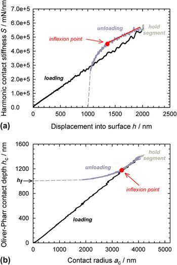
For the sake of clarity, only the results obtained on the fused silica reference material will be presented at first. The indentation with the new method delivers continuous contact stiffness data during the whole indentation test until the end of the unloading. The corresponding data are shown in Fig. 3(a). During loading, the stiffness increases linearly as a consequence of the continuously increasing contact area. The hold segment corresponds to a small increase of the stiffness at constant displacement. This means that the contact area slightly grows under constant load due to creep effects. Last, the unloading can clearly be divided into two steps: at first, the curve is linear as it was during loading. This corresponds to a removal process with a relatively slow change in contact area. The second nonlinear behavior, found after the inflexion point, corresponds to an accelerating reduction of the contact area and finally a total loss of contact. Data were collected only until 98% unloading. Since the residual depth h f is known, where final loss of contact occurs and therefore the stiffness is zero, it was possible to interpolate the missing data (dashed curve).

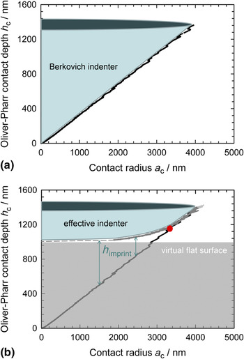
For the sake of interpretation, the contact stiffness S was transformed into the contact radius a c by Eq. (8) and the displacement into surface h was transformed into the Oliver–Pharr contact depth h c by Eq. (2). The corresponding plot is shown in Fig. 3(b). As previously explained, plotting h c versus a c during loading directly yields the shape of the Berkovich indenter, see Fig. 4(a). As expected, the included half-angle is about 70°.
h c versus a c for a Berkovich indenter in fused silica: (a) the loading segment gives access to the indenter shape and (b) the unloading (gray curve) reveals the effective indenter shape.

During unloading, the Oliver–Pharr equations are not valid for the real indenter any longer but still apply to the effective indenter. That is why plotting the knowingly invalid Oliver–Pharr contact height h c over the contact radius a c reveals the shape of the effective indenter, see Fig. 4(b). The top of the gray area corresponds to the virtual surface where the effective indenter is acting.
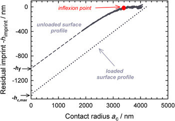
It can be seen in Fig. 3(b) that the loading segment and the initial part of the unloading segment overlap. The unloading obviously consists of two steps. At the beginning, the calculated Oliver–Pharr contact depth plotted over the contact radius lies perfectly on the loading curve. The outer part of the effective indenter has thus the same shape as the real indenter. But this also means that Eq. (9) is reduced to Eq. (2), i.e., h imprint is zero. Otherwise stated, at such distances from the center of the indent, the surface will reform to its original height after the indenter is fully removed. This implies that the red dot in Fig. 4(b) that marks the separation of both curves corresponds to the limit where a residual impression is formed. This enables the calculation of the residual contact area without any further need for imaging.
In the further progress of the unloading, the contact is described by Eq. (9), where h imprint is the vertical distance between the unloading and loading curves at each point. It corresponds to the residual plastic deformation at a certain distance away from the center; therefore, plotting −h imprint over the contact radius a c directly provides the shape of the residual impression. This is shown in Fig. 5 for fused silica and compared to the position of the rigid indenter at maximum load. It is obvious that beyond the inflexion point, the surface has not been modified, indicating the absence of plastic deformation. Further details about the shape of the residual indent will be discussed in the following paragraph.
Prediction of the shape of the residual indent from −h imprint for an indent in fused silica with a maximal displacement into surface of 2000 nm.

B. Extension to other materials
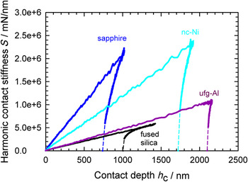
The same analysis was also conducted for the other materials. Figure 6 shows the dynamic measurements of the contact stiffness during indentation of all tested materials. Compared to fused silica, the increasingly fast decrease of the stiffness for sapphire, nc-Ni, and ufg-Al begins at a very early stage of unloading.
Contact stiffness S versus contact depth h c for all tested materials.

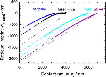
The predicted shapes of the residual impressions are plotted in Fig. 7. As expected from the load–displacement curves, the larger elastic recovery of fused silica leads to a shallower, but also narrower, imprint in the surface. The surface of nc-Ni, ufg-Al, and sapphire does not reform anywhere to its original height. In other words, the outer bound of the impression corresponds quite exactly to the edge of the indenter at the beginning of the unloading. For the metals, the residual impression is also much closer to the deformed shape of the surface at maximal load, compared to fused silica or sapphire. This explains why the contact is lost much earlier. Finally, it is observed for every material that the slope of the imprint is not purely linear, but curved outward, as expected from a higher plastic deformation under the center of the indenter than under its bounds.
Shape of the residual impression predicted from the CSM measurement. The dashed line is an extrapolation based on the knowledge of the final residual depth h f. The dotted line represents the maximal penetration of the indenter.

C. Comparison with other methods
To compare the CSM measurement with the effective indenter shape predicted by Pharr and Bolshakov,Reference Pharr and Bolshakov5 it is necessary to perform a fit of Eq. (4) to the measured unloading curve, corresponding in this study to the interval between 100 and 2% of the maximum load. This fit can also be used to calculate the values taken by the stiffness during the unloading independently from the CSM measurement. Oliver and Pharr previously showed thatReference Oliver and Pharr1:

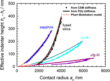
This calculated data can be used instead of the measured CSM stiffness to compute the shape of the effective indenter with Eqs. (10) and (11). This value of the stiffness derived from the load–displacement curve will be called “P(h) stiffness” in the following discussion. The results of the calculation from the CSM stiffness and the P(h) stiffness are plotted in Fig. 8 and compared with the prediction of Pharr and BolshakovReference Pharr and Bolshakov5 given by Eqs. (3), (5), and (6). For all materials, the model from Pharr and Bolshakov and the shape of the effective indenter calculated with the P(h) stiffness agree quite perfectly. This makes sense since both methods are using as input the same fit of the unloading segment of the load–displacement data.
Effective indenter shape calculated for each material by the three different methods: determination from CSM stiffness, from P(h) stiffness, and from Pharr–BolshakovReference Pharr and Bolshakov5 model. The P(h) stiffness method and Pharr–Bolshakov model yield perfectly overlapping curves.

In the case of fused silica and sapphire, the shape determined by CSM measurement is also extremely similar, albeit with a small shift. As for nc-Ni and ufg-Cu, it differs more clearly from the P(h) measurement and the Pharr and Bolshakov model.
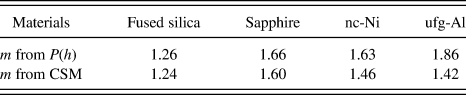
On the whole, the shapes of the effective indenters determined by the different methods appear very similar to the results of finite elements simulations already published in the literature.Reference Pharr and Bolshakov5, Reference Fischer-Cripps26 To enable further comparisons with existing data,Reference Oliver and Pharr1, Reference Fischer-Cripps26 Eq. (5) was fitted to the curves of Fig. 8, and the m exponent was calculated by Eq. (8). The results are shown in Table II. The curves obtained from the P(h) stiffness yield exactly the same m values as the fitting of Eq. (12) to the unloading segments of Fig. 2. As expected from Fig. 8, CSM- and P(h) stiffness-based methods yield very close values of m for fused silica and sapphire but more different ones for the metallic nc-Ni and ufg-Al.
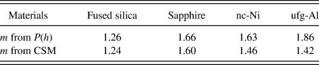
The reason is that the stiffness recorded by CSM during unloading in nc-Ni and ufg-Al is slightly higher than the calculated P(h) stiffness. An overestimation could have arisen from the CSM system experiencing technical difficulties because of the extremely fast contact area change during unloading, especially toward the end of the tip removal (see Fig. 6). To discard this potential issue, all reported experiments have been performed keeping the  ratio constant throughout the unloading ensuring an increasingly slow withdrawal.
A more likely cause for the discrepancy between CSM and P(h) stiffness originates from the different time scales associated with each method: a CSM oscillation is completed within about 15 ms, whereas the overall unloading lasts at least 1000 times longer. This implies that time-dependent processes such as plastic recovery or inverse creep are not affecting the CSM measurement but can significantly influence the shape of the unloading curve.Reference Hay, Agee and Herbert14, Reference Cheng and Cheng27 Since fused silica and sapphire did not show any significant creep during the holding segment, they should not be affected, and indeed, in both cases, a very good agreement is found between the shapes of the effective indenter determined from the CSM signal and from the P(h) stiffness data. This is why CSM seems to be a more appropriate method for testing the purely elastic response of a material and for determining the effective indenter shape without influences from the plastic recovery.
V. EXPERIMENTAL DETERMINATION OF ε FOR FUSED SILICA
The ideas developed in the first part can also be used to determine experimentally the value of ε for the Berkovich indenter, without the need for complicated calculations. Since ε should be at first considered as unknown, the reasoning has to start from the experimental observation that the residual indents left in fused silica are much smaller than the maximal contact area reached during loading. The consequence is that at the beginning of the withdrawal, the self-similarity of the indenter is preserved. Put differently, the slope of the effective indenter does not change at first, and the geometrical factor ε is the same at the beginning of the unloading than at the end of the loading. ε can thus be determined by a best-fitting procedure, using Eqs. (8) and (2) for recursively calculating the shapes of the indenter and the effective indenter. The part of the unloading that can be used for this analysis corresponds to the part before the inflexion point in Fig. 3. Indeed, SneddonReference Sneddon3 showed that S scales with h during the elastic indentation of a half-space by a conical punch so it is only the linear segment of the curve that can correspond to the full elastic recovery of the surface.
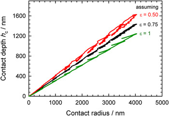
The analysis is graphically illustrated for an indentation with multiple unloadings in Fig. 9. ε is varied—which modifies the calculated contact depth h c—until the loading and unloading contact radius a c (alternatively stiffness S) coincide.
Effects of the variation of the value of ε during the fitting procedure. Note the shift of h c= h – ε · P/S that influences the agreement between loading and unloading curves.

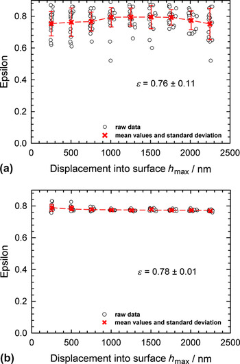
The results of the determination of ε are shown in Fig. 10(a). For comparison, the value of ε as predicted by Eq. (7) from Pharr and Bolshakov was calculated for the same set of indentations and plotted in Fig. 10(b).
Determination of ε (a) with the new fitting method and (b) using Eq. (7) from Pharr and Bolshakov model.Reference Pharr and Bolshakov5

For both methods, it appears that the value of ε does not depend on the indentation depth and is very close to the value of 0.75 initially proposed by Oliver and Pharr.Reference Oliver and Pharr1 The scattering appears to be much higher in the new method, which is likely to be caused by the use of the CSM signal. This scattering can be reduced by increasing the amplitude of the CSM oscillations, which stabilizes the signal. The clear advantage of the new method is that it relies on fewer theoretical assumptions and complicated equations. It is, however, of limited practical use since it could only be applied to fused silica. All the other materials that have been tested have indeed a too narrow band of surface that reforms totally so that a reliable fitting did not prove possible given the too limited precision of the CSM measurement.
VI. CONCLUSIONS
A new experimental method was developed to monitor the contact stiffness during nanoindentation unloading. It was shown that this new data allows a direct representation of the effective indenter introduced by Pharr and Bolshakov.Reference Pharr and Bolshakov5 Besides, it can be used to predict the shape of the residual impression and its area. This virtually removes the need for imaging for the calculation of the equivalent Vickers hardness, based on the residual area.
As an illustration of the new method, experiments were performed on different materials and an alternative procedure was introduced to measure the effective indenter shape without resorting to dynamic nanoindentation. A very close agreement with the prediction from the Pharr–Bolshakov theory was found. The results also suggest that dynamic measurement is the more accurate technique to measure contact stiffness without creep influence and should be favored for determining the effective indenter shape.
Lastly, the new theory was used to experimentally determine ε for an indentation in fused silica, leading to a value of 0.76, in very close agreement with the literature values for a rotation-symmetric paraboloid.
ACKNOWLEDGMENTS
The authors thank Dr. Erik G. Herbert from the University of Tennessee, Knoxville, for repeating some of the measurements on a different nanoindentation system. The authors also gratefully acknowledge the funding of the German Research Council, which, within the framework of its “Excellence Initiative”, supports the cluster of excellence “Engineering of Advanced Materials” at the University of Erlangen-Nürnberg.