1. Introduction
The encounter, pursuit and separation of supersonic vehicles induce a range of interference phenomena. Various types of motion between vehicles are illustrated in figure 1. Unlike the steady flow fields generated by a single vehicle in an undisturbed state, the interference flow fields resulting from multiple vehicles can impose additional aerodynamic loads on the vehicles. This may potentially lead to structural damage or cause deviations from their intended trajectories. Shock waves and shock wave interactions are common phenomena in supersonic flows. In scenarios involving multiple vehicles in relative motion, a new problem arises where the shocks of moving vehicles interfere with each other. Since the 1960s, attention has been drawn to investigating these issues of shock wave interactions.
Different types of shock wave interactions between supersonic vehicles: (a) encounter of two vehicles; (b) a high speed vehicle overtakes a low speed vehicle; (c) deployment of subvehicle; (d) a vehicle encounters a blast wave.

Research in the 1960s primarily focused on theoretical analysis and experimental measurements. Smyrl (Reference Smyrl1963) provided a closed-form solution for the flow field disturbance caused by an incident moving normal shock wave interacting with arbitrary thin airfoils and thin wedges in supersonic conditions under the small disturbance approximation (assuming the wedge or airfoil is infinitesimally thin). They also conducted experimental validation using water tunnel tests. Subsequently, the US Navy Ordnance Laboratory (Merritt & Aronson Reference Merritt and Aronson1966) carried out a series of theoretical analyses and wind tunnel experiments addressing the interference problems caused by impinging normal shock waves on various typical supersonic object shapes. The experiment produced flow field schlieren images and unsteady surface pressure curves of blunt-nosed bodies, flat-nosed cylinders,
 $60^{\circ}$
apex wedges and cones with a
 $9^{\circ}$
half-apex angle when subjected to an incident normal shock. This research also developed a theoretical approach to analyse the peak overpressure experienced at the stagnation point of blunt bodies and wedges surfaces under such conditions. Comparisons between theoretical, experimental and numerical simulation results provided by Gentry, Martin & Daly (Reference Gentry, Martin and Daly1966) demonstrated that the theoretical methods accurately predicted the peak overpressure in the disturbed region, while the numerical simulations precisely captured the surface pressure variations throughout the entire unsteady interaction process. During the same period, Nicholson (Reference Nicholson1967) extended the research scope from investigating normal incident shock waves to oblique incident shock waves and interference with sharp cones. They compared the experimental results with the theoretical outcomes for two-dimensional wedges. The findings revealed notable discrepancies between the flow field structure of three-dimensional sharp cones and the two-dimensional theoretical predictions, possibly due to pressure relief effects along the sides of the three-dimensional cones.
From the 1960s to the 1990s, several studies validated the effectiveness of computational fluid dynamics (CFD) in addressing this problem. Gentry et al. (Reference Gentry, Martin and Daly1966) employed finite difference methods to solve the unsteady interference flow field of blunt bodies and wedges with incident normal shock waves. Kutler, Sakell & Aiello used self-similar transformed Euler equations to solve the flow field structures for two-dimensional wedges (Kutler, Sakell & Aiello Reference Kutler, Sakell and Aiello1975) and three-dimensional sharp cones (Kutler & Sakell Reference Kutler and Sakell1975) under incident oblique shock wave interference. Goloviznin & Krasovskaya (Reference Goloviznin and Krasovskaya1999) utilized modern shock-capturing methods to solve the problem of interference caused by cylindrical shock waves from explosions impacting blunt wedges, providing insights into the evolution of flow field structures and surface pressure variations. Compared with wind tunnel experiments, CFD can easily achieve more detailed flow field structures, and as a result, recent theoretical studies often use CFD results as the primary reference.
Previous theoretical studies generally considered small perturbation approximations, such as extremely small wedge angles or very weak incident shock intensities. Li & Ben-Dor (Reference Li and Ben-Dor1997) extended the investigation of interactions between two-dimensional wedges and second family incident shock waves to more generalized conditions. As shown in figure 2, Li & Ben-Dor (Reference Li and Ben-Dor1997) classified three types of interference: regular interaction–regular reflection, regular interaction–Mach reflection and irregular interaction. The term `regular interaction’ refers to the normal reflection of opposite-side shock waves between the incident shock and the stationary oblique shock, which intersect directly at point
 $P$
. Conversely, `irregular interaction’ describes the Mach reflection of opposite-side shock waves between the incident shock and the stationary oblique shock, connected through a Mach stem
 $P_1 P_2$
. For regular interaction cases, the transmitted oblique shock from primary interference undergoes further reflection on the wall surface. This reflection could manifest as either regular reflection (forming regular interaction–regular reflection structure) or Mach reflection (forming regular interaction–Mach reflection structure). In figure 2,
 $T$
denotes the triple point of Mach reflection, while
 $R$
marks the intersection point between the shock and the wall. This study established critical conditions for different interference types, along with theoretical methods for calculating geometric parameters of key structures (e.g. triple points) and flow parameters in each region. Compared with previous theoretical investigations, the analytical framework proposed in that study demonstrates improved predictive accuracy over a broader range of parameter conditions.
Different types of shock-on-shock interaction considered by Li & Ben-Dor (Reference Li and Ben-Dor1997): (a) regular interaction, regular reflection; (b) regular interaction, Mach reflection; (c) irregular interaction.

The research of Li & Ben-Dor (Reference Li and Ben-Dor1997) only considered the case where the incident shock was of second family. Wang & Wu (Reference Wang and Wu2022) expanded this issue to the incident shock wave of the first family. For a first-family shock wave (selecting a coordinate system that allows the shock wave to move largely leftwards and rightwards), the pressure on the right-hand side of the shock wave is higher than that on the left-hand side, while the second-family shock wave is the opposite. More properties satisfied by the first-family shock wave will be introduced in § 2.1. During the passage of a high-speed aircraft over a low-speed aircraft, a first-family shock wave will be encountered. When the two aircraft move towards each other and pass by each other, each of them will encounter a second-family shock wave. As shown in figure 3, multiple shock interaction types are identified. When the incident shock belongs to the first family, the interference pattern between the incident shock and the oblique shock can be mapped through frame transformation to one of the six interaction types described by Edney (Reference Edney1968). Conversely, for second-family incident shocks, their interaction with the oblique shock corresponds to either Edney’s Type I or Type II interactions (equivalent to regular reflection or Mach reflection in double-wedge shock reflection). Furthermore, the secondary interaction structure emerging from the primary interaction’s propagation towards the wedge surface can be analogously treated as a pseudosteady shock reflection problem. Wang, Xu & Wu (Reference Wang, Xu and Wu2024) extended this analysis to scenarios with oblique incident shocks, specifically investigating two distinct interaction mechanisms: (i) between the incident shock and the preinteraction part of the attached shock, and (ii) between the incident shock and postinteraction part of the attached shock. This theoretical framework systematically categorizes potential interference configurations along with giving their corresponding critical conditions.
Different types of shock interaction problems and their equivalent problems. Here regular reflection (RR), Irregular reflection (IR), Mach reflection (MR), single Mach reflection (SMR), transitional Mach reflection (TMR) and double Mach reflection (DMR).

In a broader sense, the theoretical resolution of shock interaction structures and flow parameters in various regions has long been of interest to researchers. In particular, significant progress has been made in previous studies on pseudosteady shock-wave reflection problems caused by incident moving shock waves reflecting on an object (generally a sharp wedge) in a stationary flow field. Previous studies have provided the motion of triple points and the flow parameters in each region. Because of the high relevance of pseudosteady shock-wave reflection problems and the problem investigated in this paper, we will subsequently introduce these researches.
In 1971, based on experimental observations, Law (Reference Law1971) proposed a theoretical method for predicting the velocity and trajectory of triple points during the pseudosteady reflection of an incident moving normal shock wave on a sharp wedge. This work further provided theoretical calculations for the flow parameters in several interaction regions. In this study, the horizontal velocity components of the kink of transitional Mach reflection and the second triple point of double Mach reflection were assumed to match the postshock flow velocity of the incident shock wave, which later became known as the Law–Glass assumption.
Furthermore, Ben-Dor & Glass (Reference Ben-Dor and Glass1979) systematically identified the critical conditions for the occurrence of regular reflection, single Mach reflection, complex Mach reflection (now commonly referred to as transitional Mach reflection) and double Mach reflection (illustrated in figure 3), and also highlighting the influence of real gas effects on these critical conditions. In the subsequent period, a series of studies emerged addressing related issues (some of which can be classified into unsteady reflection), including experimental investigations of the impact of nitrogen dissociation on the trajectory of the second triple point in double Mach reflection (Ben-Dor & Glass Reference Ben-Dor and Glass1980); theoretical and experimental studies on the trajectory of triple points when a spherical shock wave reflects on a sharp wedge (Takayama & Sekiguchi Reference Takayama and Sekiguchi1981); theoretical analysis of triple point trajectories during planar shock reflection on inner cylindrical surfaces (Ben-Dor et al. Reference Ben-Dor, Takayama and Dewey1987b ); theoretical and experimental research on flow structures when planar shocks reflect on wedges with double inflection points (Suzuki, Adachi & Kobayashi Reference Suzuki, Adachi and Kobayashi1993).
Regarding the fundamental problem of pseudosteady shock-wave reflection of an incident moving normal shock on a sharp wedge, Li & Ben-Dor (Reference Li and Ben-Dor1995) presented a new theoretical framework for analysing the flow field structure and determining the critical conditions for various interaction types. Previous studies on this issue were often based on the Law–Glass hypothesis, which is accurate primarily when the incident shock is very strong and the wedge angle is small. However, experimental results have indicated that this assumption can lead to errors in other conditions. In this research, Li proposed an analytical theory that comprehensively considers both the shock reflection process and the airflow deflection process. This theory shows good agreement with experimental results over a wider range of parameters. Additionally, this work provided a theoretical proof of the non-existence of triple Mach reflections. This research represents a significant advancement in the classic problem of pseudosteady shock wave reflection.
To date, the fundamental problem of interacting incident moving shock waves with a sharp wedge, abstracted from shock interactions caused by relative motion in supersonic vehicles, has largely been resolved for the pseudosteady shock wave reflection subproblem with initially no flow. For the subproblem where a stationary oblique shock wave is already present due to the wedge in the initial state, the cases where the incident moving shock is of the second family have also been resolved. However, when the incident moving shock belongs to the first family, previous studies have only provided critical conditions for several major types of interactions, leaving the specific interaction structures, flow parameters in each region and the aerodynamic effects induced by these interactions as areas in need of further research.
The aim of this paper is to investigate the reflection of rightward-moving shocks of the first family over a steady oblique shock wave. Through numerical simulations combined with simplified model, we intend to explain the physics and present the interference structures. Specifically, it will illustrate the trends of the motion velocity and trajectory of the triple point, as well as the pressure in the interference region, in response to changes in the input parameters. For such a complex problem, this paper will introduce certain assumptions as in previous studies like Li & Ben-Dor (Reference Li and Ben-Dor1997) and use CFD to check these assumptions. In this paper, we only vary the wedge angle, since this allows us to cross the regions with Types II, IV, V and VI interferences, for which we are interested. This allows us to focus on the influence of one parameter.
The remainder of this paper is organized as follows. In § 2, we present the basic problem definition and numerical computation methods, and recall the critical condition theory proposed by Wang & Wu (Reference Wang and Wu2022), which serves as the foundation for subsequent analyses. Sections 3 and 4 focus on analysing the factors influencing the geometric parameters of the interaction structures (including the velocity of triple points and shock angles) and flow parameters in each region for Type VI, Type V interactions and Type II, Type IV interactions, respectively. In § 5, we integrate the analyses from § § 3 and 4 with extensive CFD simulations to qualitatively and quantitatively describe the variation of the motion of triple points and the overpressure in different regions as the wedge angle changes. This section also explains some unexpected phenomena in previous studies. In § 6 finally, we provide a summary of the entire study.
2. Problem definition, basic relations, and methods
2.1. Recall of moving shock wave reflection problems
We focus on the reflection of rightward-moving shocks of the first family over a steady oblique shock wave. As shown in figure 4(a), a sharp wedge of angle
 $\theta _w$
is initially immersed in a supersonic flow with a Mach number of
 $M_r$
, generating a stationary oblique shock with a shock angle of
 $\beta _{\textit{OR}}$
. At this point, a moving normal shock wave impinges from the left-hand side of the flow field at a speed of
 $\phi$
. This incident normal shock then collides with the stationary oblique shock, triggering a shock-on-shock interaction. In the discussion that follows, the subscript
 $l$
is used to denote the flow parameters on the left-hand side of the moving normal shock, the subscript
 $r$
for the parameters on the right-hand side and the subscript
 $d$
for the flow parameters in the region below the stationary oblique shock in the initial flow field. Additionally, we define
 $M_s = \phi / a_r$
as the Mach number characterizing the incident shock motion in the ground-fixed coordinate system.
Reflection between a rightward-moving incident shock wave and an initially steady oblique shock wave attached to a sharp wedge: (a) initial state; (b) a typical moment.

In this study, we only consider cases where the incident normal shock wave is a first-family moving shock. For a rightward-moving shock of the first family, one has
 $p_r \gt p_l$
, and in the frame comoving with the shock, the flow stream is towards the right-hand side. First-family moving shocks satisfy the shock relations as follows (Ben-Dor et al. Reference Ben-Dor, Igra, Elperin and Lifshitz2001):
 \begin{align} \phi & = M_r a_r - a_r \sqrt {\frac {\gamma +1}{2\gamma }\frac {p_l}{p_r}+\frac {\gamma -1}{2\gamma }}; \\[-34pt] \nonumber\end{align}
 \begin{align} M_l a_l & = M_r a_r - \frac {a_r}{\gamma }\left (\frac {p_l}{p_r}-1\right )\left (\frac {\gamma +1}{2\gamma }\frac {p_l}{p_r}+\frac {\gamma -1}{2\gamma }\right )^{-\frac {1}{2}}.\\[2pt] \nonumber \end{align}
Equations (2.1) and (2.2) also have equivalent forms:
 \begin{align} \phi & = M_l a_l - a_l \sqrt {\frac {\gamma +1}{2\gamma }\frac {p_r}{p_l}+\frac {\gamma -1}{2\gamma }}; \\[-34pt] \nonumber \end{align}
 \begin{align} M_l a_l & = M_r a_r - \frac {a_l}{\gamma }\left (\frac {p_r}{p_l}-1\right )\left (\frac {\gamma +1}{2\gamma }\frac {p_r}{p_l}+\frac {\gamma -1}{2\gamma }\right )^{-\frac {1}{2}}. \\[2pt] \nonumber \end{align}
Appendix A presents the proof of the equivalence between these two forms.
In the region to the left-hand side of the normal shock, a new stationary oblique shock
 $S_{\textit{NE}}$
may form under the Mach number
 $M_l$
, with a corresponding shock angle
 $\beta _{\textit{NE}}$
. Interactions can occur between the incident normal shock and both the original stationary oblique shock
 $S_{\textit{OR}}$
and the newly formed stationary oblique shock
 $S_{\textit{NE}}$
. Wang & Wu (Reference Wang and Wu2022) provided potential interaction types and critical conditions for these two sets of shocks. Here, we will recall this work as a foundation for the more detailed analysis conducted in this paper.
The basic idea behind the critical condition theory involves a coordinate transformation that converts the problem of moving shock interactions into an equivalent steady-state Edney’s six-type interaction problem (Edney Reference Edney1968). The Edney six-type interaction problem, illustrated in figure 3, describes six primary interference patterns that emerge when an incident oblique shock interacts with a bow shock induced by a blunt body at different positions. We first review the essential characteristics of these classic six interaction types identified by Edney (Reference Edney1968) and subsequent critical conditions established in later studies (Crawford Reference Crawford1973; Bramlette Reference Bramlette1974; Olejniczak, Wright & Candler Reference Olejniczak, Wright and Candler1997; Grasso et al. Reference Grasso, Purpura, Chanetz and Délery2003).
Type I and II belong to opposite side weak shock interactions. Type I occurs when the weak branch of the bow shock intersects regularly with an opposite side incident oblique shock, forming a single intersection point with an attached slip line. Type II involves Mach reflection between the two shocks, generating two triple points and two slip lines. The critical condition for transition from Type I to Type II is the detachment of the reflected shock.
Type V and VI belong to same-side weak shock interactions. Type VI features regular intersection between same-side weak shocks, typically emitting an expansion wave (or occasionally a shock) from the intersection. Type V presents greater complexity: as two same-side shocks cannot be directly connected by a single Mach stem, the extension shocks from their respective triple points must consist of one strong and one weak shock. These connect through an additional triple point, creating a three-triple-point structure. The strong shock (Mach stem) produces subsonic postshock flow, while the weak shock generates a supersonic jet between slip lines. The critical condition for transition from Type VI to Type V is when the combined shock becomes a strong shock.
Type III and IV belong to weak–strong shock interactions. When a weak incident shock interacts with a downstream strong shock (analogous to the Mach stem in standard shock reflection), the strong shock follows Mach reflection rules while the weak shock connects to the bow shock via a triple point. This creates a composite structure comprising strong shock–triple point–weak shock–triple point–strong shock. Two slip lines enclose a supersonic jet. The critical condition for transition from Type IV to Type III is when the supersonic jet, which is initially detached from the body, attaches to the body.
These classic studies reveal that interaction patterns depend on shock relationships (same/opposite side, weak/strong combination) near the intersection region. When shocks originate from different mechanisms (e.g. wedge-generated stationary shocks and moving incident shocks), their intersection can be equivalently analysed as an Edney-type interaction. Specifically, as shown in figure 4(b), defining point
 $P$
as the nominal intersection between the stationary shock
 $S_{\textit{OR}}$
and the extended incident normal shock
 $I_s$
, the interaction can be transformed into an equivalent six-type problem by adopting a coordinate system moving with
 $P$
. Here,
 $I_s$
and
 $S_{\textit{OR}}$
effectively become the two incident shocks in the Edney framework, with their relative flow parameters determining the resultant interaction type. Wang et al. (Reference Wang, Xu and Wu2024) further extended this approach to analyse interactions between
 $I_s$
and the newly formed stationary shock
 $S_{\textit{NE}}$
near their nominal intersection
 $P'$
. The velocities of point
 $P$
and
 $P'$
are derived from the motion of
 $I_s$
and the shock angle of
 $S_{\textit{OR}}$
and
 $S_{\textit{NE}}$
:
 \begin{align} \left \{\!\!\! \begin{array}{l} \boldsymbol{V_p}=\left (u_p,v_p\right )=\left (M_s a_r,M_s a_r \tan \beta _{\textit{OR}}\right )\\ \boldsymbol{V_{p'}}=\left (u_{p'},v_{p'}\right )=\left (M_s a_r,M_s a_r \tan \beta _{\textit{NE}}\right ) \end{array}. \right. \end{align}
Phase diagram of various interference types and corresponding flow fields under the condition
 $M_r = 6$
.

Through this coordinate transformation and the application of six-type critical criteria, the critical conditions for original moving shock interaction problems are established and validated via CFD simulations. Specifically, for
 $M_r = 6$
, the phase diagram showing the occurrence of various interaction types under different conditions of
 $M_s$
and
 $\theta _w$
is depicted in figure 5. In the figure, the maximum value of
 $\theta _w$
is constrained by the detachment condition corresponding to
 $M_r$
; the range of
 $M_s$
values is limited by the requirement that the incident moving shock be of the first family, given by
 \begin{equation} \sqrt {\frac {\gamma -1}{2\gamma }} \lt M_r - M_s \lt 1. \end{equation}
Thus, for
 $M_r = 6$
, the range is
 $5 \lt M_s \lt 5.622$
. Notably, since the interference between the first-family moving shock and the original stationary oblique shock typically involves same-side shock interactions or weak and strong shock interactions, only Types VI, V and IV (owing to the absence of a blunt body that distinguishes Type III from Type IV in genuine six-interaction classifications, we collectively refer to them as Type IV here) interaction types should theoretically exist. However, under certain conditions, the flow deflection angle of the equivalent problem becomes negative, indicating a ‘flow deflection angle reversal’ phenomenon. Under these circumstances, the newly generated oblique shock interferes with the moving normal shock on the opposite side, resulting in Type I and Type II interaction structures. In figure 5, the regions denoted as Type I and Type II correspond to this flow deflection angle reversal phenomenon. Figure 6 provides a clearer illustration of the flow fields for these various types of interference.
2.2. Method for numerical simulation
Various interference types and corresponding triple points.

Here
 $M_r=6,M_s=5.498,\theta _w=30^{\circ}$
Mach contours with different meshes: (a)
 $500\times 1000$
, (b)
 $2000\times 4000$
, (c)
 $4000\times 8000$
.

In this study, CFD methods are employed to obtain flow structures in the interference region. The two-dimensional unsteady Euler equations are solved using Ansys Fluent (ANSYS, Inc. 2023). A second-order upwind scheme is applied for spatial discretization; the AUSM (advection upstream splitting method) scheme (Liou Reference Liou1996) is used for numerical flux calculations; time integration is performed using a four-stage Runge–Kutta method. To ensure accuracy and stability, a fixed global maximum CFL number of 0.1 is used, with an adaptive time stepping approach.
The computations are conducted on an ideal rectangular computational domain with a uniform square grid. The initial conditions are established by first calculating a steady-state flow field based on parameters to the right-hand side of the incident normal shock wave until convergence. Subsequently, a moving normal shock is introduced in accordance with shock relations, and unsteady simulations are initiated. At any given time during the simulation, boundary conditions must be dynamically adjusted based on the actual position of the moving shock, specifically at the intersection points between the moving shock and the far-field boundaries.
To achieve sufficient resolution of shock structures in this study, three grid configurations –
 $500 \times 1000$
,
 $2000 \times 4000$
and
 $4000 \times 8000$
– were tested, with different numbers of grid points along the two dimensions to exclude irrelevant portions of the computational domain unaffected by the interference. Since the Type V interaction structure is the most complex, computations were carried out under conditions predicted to produce a Type V interaction:
 $M_r = 6$
,
 $M_s = 5.498$
and
 $\theta _w = 30^\circ$
. Figure 7 shows the Mach contour maps of the main interference region for these three grid resolutions. As illustrated, the
 $500 \times 1000$
grid resolution is insufficient to accurately resolve the supersonic jet and associated wave structures generated by the Type V interaction. The wave structures become sufficiently clear at the
 $2000 \times 4000$
grid resolution. While the
 $4000 \times 8000$
grid offers higher wave structure resolution, there are no significant changes in the key parameters, such as the location of major triple points and the angles of wave structures, compared with the
 $2000 \times 4000$
grid. Therefore, considering the trade-off between resolution and computational cost, the
 $2000 \times 4000$
grid is selected for subsequent calculations (including cases in figure 5).
2.3. Basic relations
In the following, we will frequently use the oblique shock relations, which, for brevity, will be abbreviated as (Anderson Reference Anderson2011)
 \begin{equation} M_2 = f_M\left (M_1, \beta \right ), \quad \frac {p_2}{p_1} = f_p\left (M_1, \beta \right ), \quad \frac {a_2}{a_1} = f_a\left (M_1, \beta \right ) ,\end{equation}
where
 \begin{align} f_M\left (M_1, \beta \right )& = \left (\dfrac {M_1^2+\dfrac {2}{\gamma -1}}{\dfrac {2 \gamma }{\gamma -1} M_1^2 \sin ^2 \beta - 1}+\dfrac {M_1^2 \cos ^2 \beta }{\dfrac {\gamma -1}{2} M_1^2 \sin ^2 \beta + 1}\right )^{1/2}, \\[-10pt] \nonumber \end{align}
 \begin{align} f_p\left (M_1, \beta \right ) & = 1 + \frac {2 \gamma }{\gamma +1} \big ((M_1 \sin \beta )^2 - 1\big ) , \\[-10pt] \nonumber \end{align}
 \begin{align} f_a\left (M_1, \beta \right )& = \left (\left [1 + \frac {2 \gamma }{\gamma +1} \big ((M_1 \sin \beta )^2 - 1\big )\right ] \frac {2+(\gamma -1)(M_1 \sin \beta )^2}{(\gamma +1)(M_1 \sin \beta )^2}\right )^{1/2}. \end{align}
In (2.7)–(2.10), the subscript 1 denotes the flow parameters upstream of the shock wave, and subscript 2 denotes those downstream of the shock wave;
 $\beta$
is the shock angle, which is related to the flow deflection angle
 $\theta$
by the shock angle relation:
 \begin{equation} \tan \theta = f_\theta \left (M_1, \beta \right ), \quad f_\theta \left (M_1, \beta \right ) = \frac {2\left (M_1^2 \sin ^2 \beta - 1\right )}{\left (M_1^2(\gamma + \cos 2\beta ) + 2\right ) \tan \beta }. \end{equation}
Equation (2.9) can be rearranged to provide the expression for calculating the shock angle of the oblique shock using the preshock Mach number and the pressure ratio across the shock, denoted as
 \begin{align} \beta = f_{\beta , p}\left (M_1, \frac {p_2}{p_1}\right ), \quad f_{\beta , p}\left (M_1, \frac {p_2}{p_1}\right ) = \arcsin \left (\frac {1}{M_1} \sqrt {\frac {(\gamma +1)(p_2/p_1-1)}{2\gamma } + 1}\right ). \end{align}
Substituting (2.12) into (2.11) yields the expression for calculating the flow deflection angle using the preshock Mach number and the pressure ratio, denoted as
 \begin{equation} \theta = f_{\theta , p}\left (M_1, \frac {p_2}{p_1}\right ), \quad f_{\theta , p}\left (M_1, \frac {p_2}{p_1}\right ) = \arctan \left (f_\theta \left (M_1, f_{\beta , p}\left (M_1, \frac {p_2}{p_1}\right )\right )\right ). \end{equation}
For isentropic flow along a streamline, the expressions relating the Mach number, pressure and speed of sound between two points upstream and downstream are abbreviated as
 \begin{equation} \frac {p_2}{p_1} = g_p\left (M_1, M_2\right ), \quad \frac {a_2}{a_1} = g_a\left (M_1, M_2\right ) \end{equation}
where
 \begin{align} g_p\left (M_1, M_2\right ) & = \left (\dfrac {1 + \dfrac {\gamma -1}{2}M_2^2}{1 + \dfrac {\gamma -1}{2}M_1^2}\right )^{\frac {-\gamma }{\gamma -1}} ,\end{align}
 \begin{align} g_a\left (M_1, M_2\right )& = \left (\dfrac {1 + \dfrac {\gamma -1}{2}M_2^2}{1 + \dfrac {\gamma -1}{2}M_1^2}\right )^{-\frac {1}{2}}. \end{align}
In these equations, subscripts 1 and 2 indicate points 1 and 2 along the streamline, respectively, consistent with the usage in shock relations.
Apart from shocks, Prandtl–Meyer flow occurs in some reflection types, such as Type IV. For Prandtl–Meyer flow, the Prandtl–Meyer function relates Mach numbers
 $M_1$
and
 $M_2$
at two different points along the same streamline within an expansion fan and the corresponding flow deflection angle
 $\Delta \theta$
, expressed as
 \begin{equation} \Delta \theta = \mu \left (M_2\right ) - \mu \left (M_1\right ),\, \mu \! \left (M\right ) = \sqrt {\frac {\gamma +1}{\gamma -1}} \arctan \sqrt {\frac {\gamma -1}{\gamma +1} \!\left (M^2 - 1\right )} - \arctan \sqrt {M^2 - 1}. \end{equation}
2.4. Triple point structure identification method
In the subsequent analyses and observations of the flow field in this paper, we often need to move the reference point of the coordinate system to one that follows triple points or other geometric feature points. Wang & Wu (Reference Wang and Wu2021) proposed a method for identifying moving triple points in Mach structures. However, due to the large number of triple points in this study and the complexity of frequent coordinate transformations, we have improved this method. The main improvement involves changing the original local Galilean coordinate transformation to a global self-similar coordinate transformation.
The velocity of point
 $P$
has already been precisely given by (2.5). The coordinates of point
 $P$
,
 $(x_P,y_P)$
, can be determined based on the time elapsed after the moving shock passes through the wedge leading edge. For any arbitrary point
 $(x,y)$
in the flow field, its flow velocity
 $(u,v)$
can be transformed into a self-similar system with point
 $P$
as the reference, yielding
 \begin{equation} \big (u^{(S)},v^{(S)}\big ) = \left (u - u_P \boldsymbol{\cdot }x/x_P, v - v_P \boldsymbol{\cdot }y/y_P\right ). \end{equation}
After this self-similar coordinate transformation, the flow parameters within the vicinity of any characteristic location in the flow field, such as a triple point, naturally correspond to their values in a coordinate system moving with the triple point. Consequently, a single coordinate transformation can handle all interference structures in the entire flow field. This transformation brings additional benefits, such as globally distinguishing between subsonic and supersonic flow regions and providing globally meaningful streamlines and characteristic lines.
For instance, as shown in figure 8, using streamlines in self-similar coordinates combined with Mach number contours directly confirms that triple points
 $P_2$
and
 $P_5$
share the Mach stem
 $P_2 P_5$
, while
 $I_s$
and
 $S_{\textit{NE}}$
serve as the incident shocks for the two Mach structures, respectively. This flow field data processing method will be extensively used throughout the rest of this paper.
Type II interference structures: (a) Mach contours and streamlines in self-similar coordinates, (b) schematic of the interference structure.

3. Solution of triple point motion and flow parameters for Type VI and Type V interferences
In § 2, we recalled the theoretical framework about various interaction structures and the critical conditions between them. Additionally, preliminary flow field structures for each type of interaction were demonstrated via CFD simulations. To gain a deeper understanding of the influence of problem-defining parameters on the trends in interaction structures, this section and the next will calculate the velocities and trajectories of the triple points and flow parameters, building upon the basic flow structures provided by CFD results.
We observe that the interference problems can be divided into two major categories. The first category includes Type V and Type VI interferences. These interference structures can be resolved by establishing a set of equations through the correspondence between flow directions and pressures set up by the shock wave and expansion wave relations. These equations can be solved based on the criteria of flow parallelism and pressure balance around the slip lines. (For Type V interference, it is also necessary to apply the assumptions regarding the direction of the Mach stem movement as provided by Li & Ben-Dor (Reference Li and Ben-Dor1995, Reference Li and Ben-Dor1997).)
The second category of interference problems, represented by Type II and Type IV interferences, can be approximated as one-dimensional moving shock wave reflections directly on a wall that is fixed to the flow behind the original stationary oblique shock. This approximation determines the pressure in the main regions of the interference structure, specifically the pressure behind several key shock waves. By combining the postwave pressures with the known prewave pressures and Mach numbers, the shock angles of the various shock waves can be solved, which in turn determines the velocities and trajectories of the triple points.
Due to the different physical simplifications involved, the methods for calculating the triple point velocities and flow parameters in each region vary between the two categories. This section will present the calculations for Type V and Type VI interferences, while the next section will provide the calculations for Type II and Type IV interferences.
3.1. Solution of triple point motion and flow parameters for Type VI interferences
In Type VI interaction, the incident moving shock
 $I_s$
and the stationary oblique shock
 $S_{\textit{OR}}$
intersect precisely at point
 $P$
, whose velocity and trajectory have been provided by (2.5). The flow structure near point
 $P$
is depicted in figure 9. The flow parameters for Region 0 are known. The flow between Region 0 and Region 2 satisfies the moving shock relations, while the flow between Region 0 and Region 1 satisfies the oblique shock relations, both of which can be solved straightforwardly. The task is now to solve for the flow parameters in Regions 3 and 4 after the interaction.
Type VI interference structures: (a) Mach contours and streamlines in self-similar coordinates; (b) schematic of the interference structure.

As shown in figure 9, in the coordinate system moving with point
 $P$
, Type VI interaction occurs between the incident moving shock
 $I_s$
and the stationary oblique shock
 $S_{\textit{OR}}$
. The flow in Region 2 enters Region 4 after passing through an oblique shock, and subsequently enters Region 3 after passing through two oblique shocks (
 $I_s$
and
 $S_{\textit{OR}}$
) and an expansion wave
 $C_1PC_2$
.
When the flow passes through shock
 $PB$
, the shock angle and flow deflection angle satisfy the following geometric relationships:
 \begin{align} \beta _{PB}^{(P)}& = \psi _2^{(P)} - \psi _{PB}^{(P)} ,\end{align}
 \begin{align} \theta _{PB}^{(P)}& = \psi _2^{(P)} - \psi _4^{(P)}.\end{align}
The shock angle and flow deflection angle are also constrained by the shock angle relation
 \begin{equation} \tan \theta _{PB}^{(P)} = f_\theta \left (M_2^{(P)}, \beta _{PB}^{(P)}\right ). \end{equation}
The pressures upstream and downstream of the shock satisfy the oblique shock relation
 \begin{equation} \frac {p_4}{p_2} = f_p\left (M_2^{(P)}, \beta _{PB}^{(P)}\right ). \end{equation}
When the flow passes through the expansion wave
 $C_1PC_2$
, the change in flow direction satisfies the Prandtl–Meyer relation
 \begin{equation} \psi _1^{(P)} - \psi _3^{(P)} = \nu \left (M_3^{(P)}\right ) - \nu \left (M_1^{(P)}\right ). \end{equation}
Meanwhile, the pressure satisfies the isentropic relation
 \begin{equation} \frac {p_3}{p_1} = g_p\left (M_1^{(P)}, M_3^{(P)}\right ). \end{equation}
On both sides of the slip line
 $PD_1$
, the flow satisfies the conditions of pressure equilibrium and flow direction parallel:
 \begin{align} \psi _4^{(P)}& = \psi _3^{(P)} = \psi _{PD_1}^{(P)} ,\end{align}
 \begin{align} p_4 & = p_3. \end{align}
By solving the system of equations from (3.1) to (3.8), we can determine the flow parameters in Regions 3 and 4. Overall, Type VI interactions are relatively straightforward to solve due to being regular interactions on the same side.
3.2. Solution of triple point motion and flow parameters for Type V interferences
The Type V interference structure is significantly more complex than the Type VI interaction structure, as illustrated in figure 10. In this type of interaction, multiple triple points – designated as
 $ P_1$
,
 $ P_2$
and
 $ P_3$
– and three slip lines are present. Although, in principle, the Mach stem could be a curved segment, observations from CFD results in figure 10 indicate that the Mach stem
 $ P_1 P_3$
is actually approximately a straight line. This assumption was also made by Li & Ben-Dor (Reference Li and Ben-Dor1997) when modelling interference between a second family moving shock and a stationary oblique shock. Therefore, consistent with this assumption and supported by the CFD observations, we will assume the Mach stem to be straight.
Schematic of Type V interference structure: (a) Mach contours and streamlines in self-similar coordinates; (b) schematic of the interference structure.

The velocities and directions of the three triple points
 $ P_1$
,
 $ P_2$
and
 $ P_3$
vary, requiring six parameters for description. Define the angle between the motion direction of each triple point
 $ P_i$
and the upper surface of the wedge as
 $ \chi _{P_i}$
, with a velocity magnitude of
 $ V_{P_i}$
for
 $ i = 1, 2, 3$
. In the ground-fixed coordinate system, the velocity components can be expressed as
 \begin{equation} \left (u_{P_i}, v_{P_i}\right ) = \left (V_{P_i} \cos \chi _{P_i}, V_{P_i} \sin \chi _{P_i}\right ). \end{equation}
We first analyse the geometric constraints between these six parameters. Note that since
 $ P_1$
moves along the shock
 $ S_{\textit{OR}}$
, its motion direction is given by
 \begin{equation} \chi _{P_1} = \beta _{S_{\textit{OR}}} - \theta _w. \end{equation}
If the angle between the motion direction of
 $ P_2$
and the horizontal line is
 $ \chi _{P_2}$
, since point
 $ P_2$
lies on the moving shock
 $ I_S$
, the velocity components of
 $ P_2$
can be deduced from geometric relations as
 \begin{equation} \left (u_{P_2}, v_{P_2}\right ) = \left (\frac {M_s a_r \cos \chi _{P_2}}{\cos \left (\chi _{P_2}+\theta _w\right )}, \frac {M_s a_r \sin \chi _{P_2}}{\cos \left (\chi _{P_2}+\theta _w\right )}\right ). \end{equation}
Determining the intersection of the shock segments
 $ P_2 P_3$
and
 $ P_3 P_1$
provides the location of
 $ P_3$
in relation to
 $ P_1$
and
 $ P_2$
, facilitating the derivation of their velocity relationships under the self-similar assumption
 \begin{align} u_{P_3}& = \frac {v_{P_1} - v_{P_2} + \tan \psi _{P_1 P_3} u_{P_1} - \tan \psi _{P_2 P_3} u_{P_2}}{\tan \psi _{P_1 P_3} - \tan \psi _{P_2 P_3}} ,\end{align}
 \begin{align} v_{P_3}& = -\tan \psi _{P_2 P_3} \left (u_{P_3} - u_{P_2}\right ) + v_{P_2}.\end{align}
Equations (3.10)–(3.13) provide four constraint equations among the six motion parameters for the three triple points, based on geometric constraints. Next, we transfer the coordinate system to one that moves with the three triple points and use relationships within the flow field to derive the remaining two equations.
For triple point
 $ P_1$
, where parameters in Regions 0 and 1 are known, the flow across the shock
 $ P_1C$
satisfies the geometric relationship between the shock angle and the flow deflection angle
 \begin{align} \beta _{P_1 C}^{(P_1)}& = \psi _{P_1 C}^{(P_1)} - \psi _1^{(P_1)} , \\[-10pt] \nonumber \end{align}
 \begin{align} \theta _{P_1 C}^{(P_1)} & = \psi _3^{(P_1)} - \psi _1^{(P_1)}.\end{align}
Both angles are constrained by the shock angle relations
 \begin{equation} \tan \theta _{P_1 C}^{(P_1)} = f_\theta \left (M_1^{(P_1)}, \beta _{P_1 C}^{(P_1)}\right ). \end{equation}
The pressure across the shock adheres to the oblique shock relations
 \begin{equation} \frac {p_3}{p_1} = f_p\left (M_1^{(P_1)}, \beta _{P_1 C}^{(P_1)}\right ). \end{equation}
The flow across shock
 $ P_1 P_3$
satisfies
 \begin{align} \beta _{P_1 P_3}^{(P_1)}& = \psi _0^{(P_1)} + \psi _{P_1 P_3}^{(P_1)} , \\[-10pt] \nonumber \end{align}
 \begin{align} \theta _{P_1 P_3}^{(P_1)}& = \psi _0^{(P_1)} - \psi _5^{(P_1)}.\end{align}
Also constrained by
 \begin{equation} \tan \theta _{P_1 P_3}^{(P_1)} = f_\theta \left (M_0^{(P_1)}, \beta _{P_1 P_3}^{(P_1)}\right ) ,\end{equation}
and the pressure relation
 \begin{equation} \frac {p_5}{p_0} = f_p\left (M_0^{(P_1)}, \beta _{P_1 P_3}^{(P_1)}\right ). \end{equation}
Between Regions 3 and 5, the conditions of pressure balance and parallel flow around the slip line yield
 \begin{align} \psi _3^{(P_1)}& = \psi _5^{(P_1)} , \\[-10pt] \nonumber \end{align}
 \begin{align} p_3 & = p_5.\end{align}
Equations (3.14) to (3.23) define relationships that take the velocity of point
 $ P_1$
as input and provide flow parameters surrounding
 $ P_1$
as output.
Similarly, for triple point
 $ P_2$
, with known parameters in Regions 0 and 2, the flow across shock
 $ BP_2$
satisfies
 \begin{align} \beta _{P_2 B}^{(P_2)}& = \pi - \psi _2^{(P_2)} - \psi _{P_2 B}^{(P_2)} , \\[-10pt] \nonumber \end{align}
 \begin{align} \theta _{P_2 B}^{(P_2)}& = \psi _4^{(P_2)} - \psi _2^{(P_2)}.\end{align}
Also constrained by
 \begin{equation} \tan \theta _{P_2 B}^{(P_2)} = f_\theta \left (M_2^{(P_2)}, \beta _{P_2 B}^{(P_2)}\right ) ,\end{equation}
and the pressure relation
 \begin{equation} \frac {p_4}{p_2} = f_p\left (M_2^{(P_2)}, \beta _{P_2 B}^{(P_2)}\right ). \end{equation}
Across shock
 $ P_2 P_3$
:
 \begin{align} \beta _{P_2 P_3}^{(P_2)}& = \pi - \psi _0^{(P_2)} - \psi _{P_2 P_3}^{(P_2)} , \\[-10pt] \nonumber \end{align}
 \begin{align} \theta _{P_2 P_3}^{(P_2)}& = \psi _6^{(P_2)} - \psi _0^{(P_2)}.\end{align}
Constrained by
 \begin{equation} \tan \theta _{P_2 P_3}^{(P_2)} = f_\theta \left (M_0^{(P_2)}, \beta _{P_2 P_3}^{(P_2)}\right ) ,\end{equation}
and the pressure relation
 \begin{equation} \frac {p_6}{p_0} = f_p\left (M_0^{(P_2)}, \beta _{P_2 P_3}^{(P_2)}\right ) \end{equation}
;for Regions 4 and 6, satisfying pressure balance and flow parallel
 \begin{align} \psi _4^{(P_2)}& = \psi _6^{(P_2)} ,\end{align}
 \begin{align} p_4 & = p_6. \end{align}
Equations (3.24) to (3.33) similarly define relationships around point
 $ P_2$
.
To establish the linkage between
 $ P_1$
and
 $ P_2$
via triple point
 $ P_3$
, the flow parameters for Region 6 must be determined using geometric relations to derive the shock angle for
 $ P_2 P_3$
:
 \begin{equation} \beta _{P_2 P_3}^{(P_3)} = \pi - \psi _0^{(P_3)} - \psi _{P_2 P_3}^{(P_3)} ;\end{equation}
using the oblique shock relation
 \begin{align} \theta _{P_2 P_3}^{(P_3)}& = \arctan \left (f_\theta \left (M_0^{(P_3)}, \beta _{P_2 P_3}^{(P_3)}\right )\right ) , \\[-10pt] \nonumber \end{align}
 \begin{align} \psi _6^{(P_3)}& = \psi _0^{(P_3)} + \theta _{P_2 P_3}^{(P_3)} , \\[-10pt] \nonumber \end{align}
 \begin{align} M_6^{(P_3)} & = f_M\left (M_0^{(P_3)}, \beta _{P_2 P_3}^{(P_3)}\right ).\end{align}
Pressure in Region 6 can also be found through the shock relation, but because shock
 $ P_2 P_3$
is straight and non-rotating, with Region 0 as a uniform flow region, this pressure relation is not an independent equation. The pressure for Region 6 can be retrieved directly from results around
 $ P_2$
. (The Mach number and flow direction angle for Region 6 in the
 $ P_3$
coordinate system can also be directly determined through transformation of the results around
 $ P_2$
, equivalent to calculations via (3.34) to (3.37), which are not independent.)
Once Region 6 parameters are obtained, equations around triple point
 $ P_3$
– involving shocks
 $ P_3 P_4$
and
 $ P_3 P_1$
– can again be established. Shock
 $P_3P_4$
satisfies
 \begin{align} \beta _{P_3 P_4}^{(P_3)} = \psi _6^{(P_3)} - \psi _{P_3 P_4}^{(P_3)} , \\[-10pt] \nonumber \end{align}
 \begin{align} \theta _{P_3 P_4}^{(P_3)} = \psi _6^{(P_3)} - \psi _7^{(P_3)} ,\end{align}
constrained by
 \begin{equation} \tan \theta _{P_3 P_4}^{(P_3)} = f_\theta \left (M_6^{(P_3)}, \beta _{P_3 P_4}^{(P_3)}\right ) ,\end{equation}
and the pressure relation
 \begin{equation} \frac {p_7}{p_6} = f_p\left (M_6^{(P_3)}, \beta _{P_3 P_4}^{(P_3)}\right ). \end{equation}
While across shock
 $ P_1 P_3$
,
 \begin{align} \beta _{P_1 P_3}^{(P_3)} = \psi _0^{(P_3)} + \psi _{P_1 P_3}^{(P_3)} , \\[-28pt] \nonumber \end{align}
 \begin{align} \theta _{P_1 P_3}^{(P_3)} = \psi _0^{(P_3)} - \psi _5^{(P_3)} ,\\[2pt] \nonumber \end{align}
constrained by
 \begin{equation} \tan \theta _{P_1 P_3}^{(P_3)} = f_\theta \left (M_0^{(P_3)}, \beta _{P_1 P_3}^{(P_3)}\right ) ,\end{equation}
and the pressure relation
 \begin{equation} \frac {p_5}{p_0} = f_p\left (M_0^{(P_3)}, \beta _{P_1 P_3}^{(P_3)}\right ) ;\end{equation}
between Zones 5 and 7, maintains pressure and flow parallel conditions
 \begin{align} \psi _5^{(P_3)}& = \psi _7^{(P_3)} , \\[-12pt] \nonumber \end{align}
 \begin{align} p_5 & = p_7. \end{align}
Equations (3.34) to (3.47) link triple points
 $ P_1$
and
 $ P_2$
via
 $ P_3$
, establishing velocity constraints. With these constraints and geometric constraints fully used, closure of the set of equations needs to be examined before solving. Given its size, its closure is not immediately obvious, so we simplify for better insight.
Now we simplify the system into four variables: the velocities of
 $ P_1$
and
 $ P_2$
,
 $ V_{P_1}$
and
 $ V_{P_2}$
, and pressures in Zones 3 and 5, 7,
 $ p_3$
and
 $ p_4$
. Equations (3.9) and (3.11) yield velocity components when
 $ P_1$
and
 $ P_2$
velocity magnitudes are known, determining flow speed, Mach numbers and directions in Zones 0, 1 and 2 in
 $ P_1$
and
 $ P_2$
systems. To derive
 $ P_3$
velocity, use
 $ p_3$
,
 $ p_4$
to calculate the shock angles
 $ P_1 P_3$
,
 $ P_2 P_3$
, then solve using geometric relations
 \begin{align} \psi _{P_1 P_3}& = f_{\beta , p}\left (M_0^{(P_1)}, \frac {p_3}{p_0}\right ) - \psi _0^{(P_1)} , \\[-10pt] \nonumber \end{align}
 \begin{align} \psi _{P_2 P_3} & = \pi - f_{\beta , p}\left (M_0^{(P_2)}, \frac {p_4}{p_0}\right ) - \psi _0^{(P_2)}. \\[9pt] \nonumber \end{align}
Then find
 $ P_3$
velocity using (3.12).
Around point
 $ P_1$
, reduce (3.14) to (3.23) into a flow deflection angle equation around the slip line:
 \begin{equation} \psi _2^{(P_2)} + f_{\theta , p}\left (M_2^{(P_2)}, \frac {p_4}{p_2}\right ) = \psi _0^{(P_2)} + f_{\theta , p}\left (M_0^{(P_2)}, \frac {p_4}{p_0}\right ). \end{equation}
Similarly, for
 $ P_2$
, reduce (3.24) to (3.33) into
 \begin{equation} \psi _2^{(P_2)} + f_{\theta , p}\left (M_2^{(P_2)}, \frac {p_4}{p_2}\right ) = \psi _0^{(P_2)} + f_{\theta , p}\left (M_0^{(P_2)}, \frac {p_4}{p_0}\right ). \end{equation}
For
 $ P_3$
, calculate Zone 6 flow using (3.34) to (3.37), then simplify (3.24) to (3.33) into
 \begin{equation} \psi _6^{(P_3)} - f_{\theta , p}\left (M_6^{(P_3)}, \frac {p_3}{p_4}\right ) = \psi _0^{(P_3)} + f_{\theta , p}\left (M_0^{(P_3)}, \frac {p_3}{p_0}\right ). \end{equation}
Equations (3.50) to (3.52) encompass all previously mentioned equations describing triple point motion and flow parameters, leading to a simplified yet under-determined system: four unknowns are governed by only three equations, requiring an additional equation for solution.
The choice of this additional equation can be heuristic. In a series of previous studies on pseudosteady shock reflection or related problems (Law Reference Law1971; Ben-Dor Reference Ben-Dor1981; Takayama & Sekiguchi Reference Takayama and Sekiguchi1981; Ben-Dor et al. Reference Ben-Dor, Dewey and Takayama1987a
), and Li & Ben-Dor (Reference Li and Ben-Dor1997) on second-family moving shock reflections, researchers often assume the Mach stem to be perpendicular to the wedge surface. For pseudosteady shock reflection, the trajectory of the nominal intersection point between the incident shock and the wedge surface corresponds to the main motion direction of the interference structure, and the previous assumption was that the Mach stem was perpendicular to this motion direction. In this problem, the nominal intersection point
 $P$
of the incident shock
 $I_s$
and the oblique shock
 $S_{\textit{OR}}$
also corresponds to the main motion direction of the interference structure. Therefore, we adopt an extended assumption: the flow in Region 0, relative to
 $ P$
, is perpendicular to Mach stem
 $ P_1 P_3$
:
 \begin{equation} \psi _0^{(P)} + \psi _{P_1 P_3} = \pi / 2. \end{equation}
Previous studies usually directly adopted this assumption to conduct theoretical analysis. In this paper, we present the actual situation here. Figure 11 illustrates the Type V interference structure and shows the Mach stem and streamlines within the
 $ P$
-based system. The CFD results indicate that the flow in Region 1 is indeed approximately perpendicular to the Mach stem in the
 $ P$
point coordinate system.
Mach contours and streamlines in
 $ P$
-point coordinates for Type V interference: (a)
 $ M_r = 6, M_s = 5.498, \theta _w = 30^\circ$
, (b)
 $ M_r = 6, M_s = 5.498, \theta _w = 26^\circ$
.

Therefore, for Type V interactions, utilizing this assumption allows the system of equations to be closed, enabling the computation of triple point velocities and flow parameters in each disturbance region. In § 5, we will apply the methods presented in this section to compute the velocities and trajectories of the triple points in Type VI and Type V interferences, as well as the variation of overpressure in the interference region with changes in the wedge angle.
4. Solution of triple point motion and flow parameters for Type II and Type IV interferences
4.1. Method for calculating pressure in subsonic region
Now we turn to Type I, Type II and Type IV interferences. Deflection angle reversal phenomenon occurs when the wedge angle
 $\theta _w$
is below a certain critical threshold. In such cases, the newly formed stationary oblique shock
 $S_{\textit{NE}}$
and the incident moving shock
 $I_s$
act as the incident shocks in a cross-side shock interaction. Logically, this situation could be approached similarly to Type V and Type VI interferences by establishing equations of pressure balance and flow parallelism around the point
 $P'$
. This method is indeed feasible in practice. Type I interference, being a regular reflection, is relatively straightforward to solve. Type II interference can be approached using previously established methods, with the assumption of a straight Mach stem. Given the symmetry of this method with the approach in § 3.2 (wherein Type II is simpler than Type V), we will not provide a detailed discussion here.
Here, we introduce an entirely new perspective. Figure 8 illustrates the Mach structure formed between
 $S_{\textit{NE}}$
and
 $I_s$
under Type II conditions. Comparing figure 8 with Type IV structures in figure 5(c) or figure 12, Type V in figure 5(b) and Type VI in figure 5(a), it is noticeable that the Mach stem
 $P_2 P_5$
consistently exists. However, as the wedge angle
 $\theta _w$
increases, the stem’s curvature intensifies, making it challenging to maintain the assumption that the Mach stem is linear. This structural similarity raises the question: Is there a unified physical mechanism governing the flow state near the Mach stem
 $P_2 P_5$
?
In § 3.2, within a moving coordinate system near interference regions, the flow field of the Type VI interference is entirely supersonic. Although Type V interference has a subsonic region behind the Mach stem, most of the regions are supersonic. This supersonic-dominated flow allows us to use established theories of steady supersonic shock interactions to establish constraint equations for solving interference structures. However, for the Mach structure formed between
 $S_{\textit{NE}}$
and
 $I_s$
, the subsonic region is large, and the curvature of the Mach stem
 $P_2 P_5$
is significant, rendering stationary shock interaction theories difficult to apply. It seems that resolving this issue may require numerical methods to solve elliptical equations in the subsonic region or the full Euler equations.
Mach contours and relative streamlines of Zone 10 with respect to Zone 2 when
 $\theta _w = 22^{\circ }$
.

This paper attempts to offer a physically intuitive approach. Although it is an approximate method and not fully exact, we will show that its results are generally consistent with CFD, allowing the capture of qualitative trends and the revelation of underlying physics. Consider a one-dimensional problem of a moving shock reflecting off a stationary wall. Before and after the shock reflection, the fluid between the shock and the wall remains stationary relative to the wall. For this subsonic region, with a Mach number of zero, all flow parameters can be calculated using known parameters on the opposite side of the shock and the moving shock relations. From the perspective of moving shock reflection, the subsonic region is solvable. We now attempt to redefine the current problem as one of moving shock reflection.
As illustrated in figure 12, the problem of the first-family moving shock reflecting on a stationary oblique shock can be viewed as an interference issue between
 $I_s$
and either
 $S_{\textit{OR}}$
or
 $S_{\textit{NE}}$
, as well as a shock reflection issue where the high-speed gas in Zone 2 upstream of shock
 $I_s$
‘strikes’ Zone 1. Despite the influence of the interference structures near points
 $P$
or
 $P'$
, the flow parameters in Zone 1 and those behind the Mach stem
 $P_2 P_5$
are not identical. However, the CFD results in figure 12 reveal that point
 $P$
or
 $P'$
primarily extends slip lines into the region behind Mach stem
 $P_2 P_5$
. From a one-dimensional perspective orthogonal to the slip line, the slip line behaves like a contact discontinuity, with consistent velocities of the gases on both sides. Hence, the relative velocity between Zones 1 and 2 can be seen as the difference in gas flow velocities across the moving shock. Consequently, the pressure
 $p_{10}$
behind the Mach stem
 $P_2 P_5$
can be solved using the moving shock compatibility relation and the known flow parameters in Zone 2:
 \begin{equation} \sqrt {(u_1-u_2)^2+(v_1-v_2)^2} = \frac {a_2}{\gamma }\left (\frac {p_{10}}{p_2}-1\right )\left (\frac {\gamma +1}{2\gamma }\frac {p_{10}}{p_2}+\frac {\gamma -1}{2\gamma }\right )^{-\frac {1}{2}}. \end{equation}
With the pressure behind the Mach stem
 $P_2 P_5$
, it is relatively straightforward to calculate other interference structure parameters. Since this assumption can directly calculate the pressure in Zone 10, the CFD results presented in the subsequent § 5.3, especially figure 13, serve as a check of this assumption. Therefore, no additional checks will be conducted here.
4.2. Solution of triple point motion for Type II and Type IV interferences obtained from pressure in the subsonic region
Changes in interference structures with wedge angle: (a) velocity of triple points; (b) trajectory angles of triple points; (c) pressure in interference regions.

Upon determining
 $p_{10}$
, the solutions for the triple points
 $P_2$
and
 $P_5$
involved in Type II and Type IV interferences can be obtained relatively easily. The solution process involves setting equations of pressure balance and flow parallelism around the slip lines of the triple points, which are similar to those in § 3.2, so we directly present the simplified final equations.
For triple point
 $P_5$
, the path must follow the newly formed oblique shock
 $S_{\textit{NE}}$
, requiring only one parameter: the velocity magnitude
 $V_{P5}$
. Upon simplification, the resulting equation is
 \begin{equation} \psi _2^{(P_5)} \pm f_{\theta ,p}\left (M_2^{(P_5)}, \frac {p_{10}}{p_2}\right ) = \psi _8^{(P_5)} + f_{\theta ,p}\left (M_8^{(P_5)}, \frac {p_{10}}{p_8}\right ). \end{equation}
The
 $\pm$
sign represents either a positive or inverse Mach structure. Except for the critical condition where the Mach stem is a normal shock, only one equation will have a solution. In practical solutions, attempts are made to solve both equations using Newton iteration, with the successful convergence indicating the correct equation.
For triple point
 $P_2$
, which is located on the moving shock
 $I_s$
, specifying the velocity magnitude
 $V_{P2}$
allows the trajectory to be expressed geometrically as
 \begin{equation} \chi _{P2} = \arccos \frac {\phi }{V_{P2}} - \theta _w. \end{equation}
Subsequently, pressure balance and flow parallelism equations over the slip lines of the triple point can be formulated, with the final simplified form being
 \begin{equation} \psi _2^{(P_2)} \pm f_{\theta ,p}\left (M_2^{(P_2)}, \frac {p_{10}}{p_2}\right ) = \psi _0^{(P_2)} - f_{\theta ,p}\left (M_0^{(P_2)}, \frac {p_{10}}{p_0}\right ). \end{equation}
As in (4.2), here the
 $\pm$
sign corresponds to the type of Mach structure too. Thus, we provide a method for calculating the velocities of each triple point and the flow parameters of major interference regions using the defining parameters of the problem (
 $M_r, M_s, \theta _w$
). In § 5, we will apply the methods presented in this section to calculate the velocities and trajectories of the triple points in Type II and Type IV interferences, as well as the variation of overpressure in the interference region with changes in the wedge angle. Additionally, we will tentatively extend the application of this method to Type V interference.
4.3. Summary of model approximation assumptions
So far, this paper has provided methods for calculating the velocities, trajectories of triple points, and overpressure in the interference regions for various types of interactions through careful observation of the CFD flow field. Here, we summarize the basic assumptions and solution logic used in the computational methods corresponding to each type of interference (see table 1).
Summary of model approximation assumptions.

For Type VI interference, it is a regular reflection of the same-side shock wave, and no additional assumptions are needed. The incident moving normal shock wave
 $I_s$
directly intersects with the original stationary oblique shock wave
 $S_{\textit{OR}}$
at point
 $P$
. The motion velocity and trajectory of point
 $P$
are completely constrained by the shock angle of
 $S_{\textit{OR}}$
and the velocity of
 $I_s$
through geometric relations. Next, we only need to solve the pressure balance and flow parallelism equations around the slip line in the coordinate system of point
 $P$
to obtain the flow parameters in each region. Type I interference also belongs to the regular reflection of the opposite-side shock wave and similarly does not require additional assumptions.
For Type V interference, this paper refers to the assumption that the Mach stem is a straight line and perpendicular to the wall, which is often used in the studies of pseudosteady and unsteady shock reflections by Li & Ben-Dor (Reference Li and Ben-Dor1995, Reference Li and Ben-Dor1997). Combined with observations from the CFD results, we assume that the Mach stem in Type V interference is a straight line and that it behaves as a normal shock in the coordinate system moving with point
 $P$
. This assumption, along with the pressure balance and flow parallelism equations written around the slip lines in the three triple point coordinate systems, allows us to simultaneously solve for the motion velocities and trajectories of the three triple points, as well as the flow parameters in each region.
For Type II and Type IV interference, this paper notes from the observation of CFD results that the incident moving normal shock wave approximately undergoes one-dimensional shock reflection on a wall fixed to the flow in Region 1. By applying the compatibility relation of moving shock waves between Regions 1 and 2, we can directly obtain the pressure in the interference region, which corresponds to the pressures on both sides of the slip lines extending from the triple points
 $P_2$
and
 $P_5$
. Given this pressure, we can then solve for the motion velocities of the triple points and other flow parameters in each region by writing the pressure balance and flow balance equations.
5. Analysis of parametric trends in interference structures
5.1. Selection of parameter range
This section utilizes the computational methods provided in § § 3 and 4, combined with CFD simulations, to elucidate the changes of primary interference structures with variations in wedge angle. The methods from § § 3 and 4 mainly serve to reveal influencing factors and trends, while the CFD simulations offer quantitatively accurate results.
As shown in figure 5, altering the wedge angle
 $\theta _w$
under given
 $M_r$
and
 $M_s$
conditions not only results in quantitative changes to interference structures but can also lead to qualitative shifts in structure types. Therefore, to highlight the two physical mechanisms of flow deflection and moving shock reflection proposed in this paper,
 $M_r = 6$
and
 $M_s = 5.498$
are held constant, with
 $\theta _w$
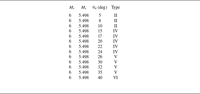
as the varying parameter for parametric analysis. Table 2 lists the conditions selected for CFD calculations, where multiple states are chosen for each type of interference except for the relatively simple Type VI.
Parametric analysis cases.

During the parametric analysis, the focus is mainly on the velocity and trajectory angles of the triple points and the pressure behind the interference structures. The first two are important parameters of the interference structure, while the latter reflects the additional pressure increase due to the interference, providing a reference for analysing aerodynamic loads on the object.
5.2. Trends in interference structures for Type VI and Type V interferences
Changes in interference structures with wedge angle: (a) velocity of triple points; (b) trajectory angles of triple points; (c) pressure in interference regions.

We first analyse the trends in shock interference structures for Type VI and Type V interferences as the wedge angle changes. Figure 14 presents theoretical calculations and CFD parametric analysis results for these states. In Type VI interference, the triple points merge into the actual intersection
 $P$
of the incident shock
 $I_s$
and original stationary oblique shock
 $S_{\textit{OR}}$
. The pressure near the slip line extending from point
 $P$
(designated as Region 3 in the schematic of figure 9) represents the pressure behind the interference structure. In Type V interference, as shown in figure 10, there are three freely moving triple points,
 $P_1, P_2, P_3$
. Meanwhile, there are two equal pressure regions: near the slip lines extending from
 $P_2$
to Regions 4 and 6, and from
 $P_1, P_3$
to Regions 3, 5, 7. The analysis targets these triple points and equal pressure regions.
As shown in figures 14(a) and 14(b), as the wedge angle increases, the velocities and directions of the three triple points tend to converge, causing the Type V structure to gradually merge into a Type VI structure. Theoretical calculations also show a tendency for the velocities of the triple points to converge. Compared with CFD results, there is a quantitative discrepancy in theoretical calculations, with the greatest error in triple point velocity magnitude approaching 10 % and in trajectory angles reaching 15 %.
The interference region pressure displayed in figure 14(c) shows more intriguing characteristics. Both theoretical and CFD results indicate that during the transition from Type V to Type VI interference, the pressure does not change continuously. Instead, it increases with the wedge angle, with the peak pressure in Type V interference being several times that in Type VI. This local anomalously high pressure, transmitted to the wall via a series of wave systems, could lead to additional aerodynamic loads on the object’s surface, potentially requiring consideration in engineering applications.
Two notable observations emerge from figures 14(a) and 14(b). First, the theoretical calculations for triple point velocities in figure 14(a) fail to fully converge to Type VI conditions, unlike the CFD results. Second, the trajectory of
 $P_2$
in figure 14(b) appears non-convergent. We analyse the causes of these discrepancies below.
Figure 15 presents Mach number contours and streamlines in the
 $P$
-point coordinate system for
 $\theta _w = 32^\circ$
and
 $\theta _w = 35^\circ$
. The results demonstrate significant flow deflection downstream of the Mach stem
 $P_1 P_3$
, whereas our analysis in § 3.2 assumed the Mach stem
 $P_1 P_3$
to behave as a normal shock. This assumption leads to overestimation of the post-Mach-stem pressure (evident in Regions 3, 5 and 7 in figure 14
c), which consequently inflates the calculated propagation speed of shock
 $P_1 P_3$
in the laboratory frame. Simultaneously, the pressure overestimation and geometric deviations caused by approximating the oblique shock as normal contribute to exaggerated trajectory angles for
 $P_2$
and
 $P_3$
. Collectively, these factors account for the observed discrepancies between theoretical calculations and CFD results in Type V interference.
Mach contours and streamlines in
 $ P$
-point coordinates for Type V interference: (a)
 $ M_r = 6, M_s = 5.498, \theta _w = 32^\circ$
, (b)
 $ M_r = 6, M_s = 5.498, \theta _w = 35^\circ$
.

5.3. Trends in interference structures for Type II and Type IV interferences
Next, we analyse the changes in shock interference structures for Type II and Type IV interferences as the wedge angle increases. Figure 13 displays the theoretical and CFD results for the velocities, trajectory angles of triple points
 $P_2, P_5$
, and the pressure behind the Mach stem
 $P_2 P_5$
. Notably, the computation method provided in § 4 was established specifically for Type II and Type IV interferences, corresponding to the phase diagram range with
 $\theta _w \lt 24.2^\circ$
. For larger wedge angles, the method in § 4 is theoretically inapplicable. However, as noted in § 4.1, Type V and Type VI interferences also show interactions between
 $S_{\textit{NE}}$
and
 $I_s$
, forming a Mach stem
 $P_2 P_5$
. Thus, figure 13 presents extrapolated theoretical and CFD results.
First, considering only the theoretically applicable range, i.e.
 $\theta _w \lt 24.2^\circ$
, the results in figure 13 demonstrate that as
 $\theta _w$
increases, both the trajectory angles of triple points
 $P_2$
and
 $P_5$
increase; the velocity of
 $P_2$
increases while the velocity of
 $P_5$
decreases; and the pressure behind the Mach stem
 $P_2 P_5$
in Region 10 consistently rises. The increase in pressure in Region 10 with increasing wedge angle is intuitive, and the rising pressure in Region 10 drives the velocities of triple points
 $P_2$
and
 $P_5$
to increase and decrease, respectively. The rise in trajectory angles results from the synchronous increase in shock angles
 $S_{\textit{NE}}$
and
 $S_{\textit{OR}}$
due to the growing wedge angle. The theoretical calculation results accurately calculate the velocities of the triple points and trajectory angles for
 $P_5$
and the pressure in Region 10, though error exists in calculating the trajectory angle for
 $P_2$
.
For
 $\theta _w \gt 24.2^\circ$
, as seen in figure 13, theoretical solutions for the velocity of
 $P_5$
and its and trajectory angles maintain high precision, but solutions for pressure in Region 10 and the velocity of
 $P_2$
shows a systematically growing error, and solutions for the trajectory angle of
 $P_2$
trend incorrectly. Figure 16 helps explain these phenomena. In Type VI interference, a known expansion wave
 $C_1 P C_2$
directed towards the wall is produced, as shown in figure 16(a), while in Type V interference depicted in figure 16(b), neglecting its finer structure, a similarity exists with Type IV interference resulting in a final expansion wave. This expansion wave, after reflecting off the wall, penetrates the slip line from the region near point
 $P$
, disrupting the uniform pressure in Region 10. The presence of this expansion wave invalidates the assumption of using the relative velocity of Zone 1 to Zone 2 to estimate the velocity of Zone 10 relative to Zone 2. Consequently, the computation of velocity parameters of
 $P_2$
and the pressure in Region 10 (where CFD data is sampled near point
 $P_2$
) becomes inaccurate. However, point
 $P_5$
remains largely unaffected due to its greater distance from point
 $P$
, hence solutions for its velocity and trajectory remain accurate.
Pressure contours around point
 $P$
: (a)
 $\theta _w=40^\circ$
; (b)
 $\theta _w=35^\circ$
.

As shown in figure 13, noticeable discrepancies persist between the theoretically calculated trajectory angle
 $\chi _{P2}$
of triple point
 $P_2$
and CFD results at smaller wedge angles. To investigate this divergence, we hypothesize that the primary source of error stems from deviations between the calculated pressure in Region 10 (derived from the assumptions in this study) and the actual pressure distribution. Although the pressure differences between theoretical and CFD results in figure 13(c) appear modest, the trajectory of
 $P_2$
exhibits critical sensitivity to pressure variations. Consequently, even minor pressure discrepancies ultimately lead to significant trajectory deviations.
To validate this hypothesis, we replaced the pressure values computed via (4.1) with the CFD-derived pressures from figure 13(c) and recalculated the velocities and trajectory angles of
 $P_2$
and
 $P_5$
. As shown in the figure 17, after the calculation using the pressure provided by CFD, when the wedge angle
 $\theta _w$
is small, the trajectory angle of
 $P_2$
is basically consistent with the CFD result. When
 $\theta _w$
is appropriately increased, it also has a general trend consistent with the CFD result. When
 $\theta _w$
is large, the pressure near the slip lines extended from the triple points
 $P_2$
and
 $P_5$
will gradually differ. Therefore, the calculation for the case with a larger wedge angle (which can be clearly seen from figure 16) was not carried out. This computational verification confirms that the observed errors in the Type II/IV model primarily arise from pressure estimation inaccuracies in Region 10, thereby substantiating our hypothesis.
5.4. Reviewing the critical conditions from the perspective of triple points
In CFD simulations, some special cases emerged where the actual interference types differed from those predicted by previous studies. These discrepancies can be explained from the perspective of triple points, as elaborated in this section.
The interference structures calculated using CFD-derived pressure data: (a) velocity of triple points; (b) trajectory angles of triple points.

Triple points forming various interference structures.

According to the critical condition calculation method recalled in § 2, Type IV interference is expected at
 $\theta _w = 22^\circ$
. However, as shown in figure 12, the CFD results actually indicate Type V interference. The reason for this discrepancy lies in the theoretical method’s sole reliance on identifying the type of shock
 $S_{\textit{OR}}$
at point
 $P$
in the coordinate system, which may still appear as a strong shock at point
 $P_1$
due to the velocity difference. This results in an actual Type V interference configuration.
Reviewing the critical conditions between interference types from the perspective of triple points, figures 6 and 18 illustrate the four primary triple points (
 $P_1, P_2, P_3, P_5$
) and their respective interference structures. In Type V scenarios, all four points coexist, delineating three segments of weak shocks (
 $S_{\textit{NE}}, P_2 P_3, S_{\textit{OR}}$
) and two segments of strong shocks (
 $P_5 P_2, P_3 P_1$
). Increasing
 $\theta _w$
will cause the merger of points
 $P_1, P_3, P_2$
into point
 $P$
, transitioning Type V to Type VI interference. Conversely, decreasing
 $\theta _w$
transforms
 $S_{\textit{OR}}$
into a strong shock, unable to smoothly connect with the strong shock
 $P_3 P_1$
through a triple point, leading to the disappearance of
 $P_1$
and conversion to Type IV. Further reduction of
 $\theta _w$
causes
 $P_2 P_3$
to also become a strong shock, resulting in
 $P_2 P_3$
and
 $P_3 P_1 S_{\textit{OR}}$
directly connecting as strong shocks, causing
 $P_3$
and its supersonic jet structure to vanish, shifting the type to Type II or even Type I. Additionally, due to the persistent crossing relationship between
 $I_s$
and
 $S_{\textit{NE}}$
, structures similar to Type II with triple points
 $P_2$
and
 $P_5$
are also present in Types IV, V and VI.
6. Conclusion
This study investigates the reflection of a rightward-moving shock wave on a stationary oblique shock generated by a wedge, abstracting the relative motion between supersonic vehicles. To gain deeper insight into this complex problem, we adopt a combined approach of CFD and theoretical analysis. The theoretical framework provides qualitative trends of interference structures, such as triple-point velocities and overpressure variation with wedge angle, while CFD verifies the key assumptions of the theory and delivers quantitatively accurate results.
As the wedge angle decreases, we obtain the following results.
-
(i) For Type VI interference, when interpreted in a moving frame attached to the nominal intersection point, the interference reduces to a steady configuration. A smaller wedge angle decreases the oblique shock angle, leading to reductions in overpressure, trajectory angle and velocity.
-
(ii) For Type V interference, the incident and stationary shocks are connected through three triple points and a Mach stem. Here the Mach stem acts effectively as a normal shock in the moving frame. As the wedge angle decreases, triple-point velocities and overpressure decline, but the sudden emergence of the Mach stem at the VI–V transition generates a strong local compression and produces a sharp pressure spike. This highlights the role of new strong shocks in governing transition process.
-
(iii) For Types IV and Type II interferences, these can be approximated by the reflection of a moving normal shock. The weakening of effective reflection strength with smaller wedge angles directly lowers the interaction-region pressure. With this pressure known, triple-point dynamics follow consistently from triple-point theory, showing convergence of velocities. This analogy also explains why the triple point linked to the newly generated oblique shock accelerates as the wedge angle decreases.
Furthermore, we find that the transition between interference types can be interpreted through the emergence and disappearance of triple points. The effective critical conditions are determined in coordinate systems moving with the triple points, which may differ slightly from the nominal intersection point of the incident and stationary shocks.
Overall, the study clarifies how wedge angle regulates the strength and dynamics of moving-shock–oblique-shock interactions through triple-point mechanisms and shows the value and limitations of simplified model. This paper was limited to a particular choice of the inflow and shock Mach numbers. Should other choices yield new physical findings beyond quantitative variations, they would merit further investigation. While the analysis focused on primary interference structures and neglected viscosity and the interaction with the wedge surface, these aspects can be analysed in future research.
Acknowledgements
The authors are grateful to all referees for their valuable comments that helped to improve the manuscript. This work was supported by the National Key Project (grant no. GIXM92579). This work was also supported by the National Natural Science Foundation of China (grant no. 12402269). The authors also wish to thank the support from Qinghang Scholar Funding Program and National Postdoctor a Researcher Funding Program (no. GZC20240846). The authors used ChatGPT (GPT-5, OpenAI) for language editing. The tool was used solely for linguistic purposes, and the authors remain responsible for all scientific content.
Declaration of interests
The authors report no conflict of interest.
Appendix A. Two forms of shock relations
Referring to the results presented by Ben-Dor et al. (Reference Ben-Dor, Igra, Elperin and Lifshitz2001), the shock relations for first-family moving shocks exhibit two equivalent formulations: (2.1) and (2.2) constitute the first form, while (2.3) and (2.4) represent the second. Building upon existing theoretical derivations, we provide a direct proof of their equivalence below.
Consider a first-family shock in its attached coordinate system. The upstream/downstream pressures, Mach numbers and densities satisfy the Rankine–Hugoniot equations
 \begin{align} \frac {p_r}{p_l}&=\frac {2 \gamma \big(M_l^\phi \big)^2-(\gamma -1)}{\gamma +1} , \\[-12pt] \nonumber \end{align}
 \begin{align} \big (M_r^\phi \big )^2 & =\frac {1+\left (\frac {\gamma -1}{2}\right )\big(M_l^\phi \big)^2}{\gamma \big(M_l^\phi \big)^2-\frac {\gamma -1}{2}} ,\\[-12pt] \nonumber \end{align}
 \begin{align} \frac {\rho _r}{\rho _l}&=\frac {(\gamma +1)\big(M_l^\phi \big)^2}{2+(\gamma -1)\big(M_l^\phi \big)^2} , \\[10pt] \nonumber \end{align}
where
 $ M_l^\phi$
and
 $ M_r^\phi$
denote the Mach numbers in the shock-attached frame for left-hand (upstream) and right-hand (downstream) flows, respectively.
Rearranging (A2) by transposing its denominator yields
 \begin{equation} \gamma \big (M_r^\phi \big )^2\big(M_l^\phi \big)^2-\frac {\gamma -1}{2}\big(M_l^\phi \big)^2-\frac {\gamma -1}{2}\big (M_r^\phi \big )^2=1. \end{equation}
The complete symmetry of (A4) permits inverse transformation from (A2), generating its dual form,
 \begin{equation} \big(M_l^\phi \big)^2=\dfrac {1+\left (\dfrac {\gamma -1}{2}\right )\big (M_r^\phi \big )^2}{\gamma \big (M_r^\phi \big )^2-\dfrac {\gamma -1}{2}}. \end{equation}
Substituting (A5) into (A1) produces
 \begin{equation} \dfrac {p_r}{p_l}=\dfrac {2 \gamma \dfrac {1+\left (\dfrac {\gamma -1}{2}\right )\big (M_r^\phi \big )^2}{\gamma \big (M_r^\phi \big )^2-\dfrac {\gamma -1}{2}}}{\gamma +1}+1. \end{equation}
Simplification yields the pressure ratio’s dual expression
 \begin{equation} \frac {p_r}{p_l}=\frac {\gamma +1}{2 \gamma \big (M_r^\phi \big )^2-(\gamma -1)}. \end{equation}
In the laboratory frame, the shock propagation velocity equals the downstream flow velocity minus the shock-relative velocity:
 \begin{equation} \phi =M_r a_r-\big (M_r^\phi \big ) a_r. \end{equation}
Equivalently, it can be expressed through upstream parameters:
 \begin{equation} \phi =M_l a_l-\big(M_l^\phi \big) a_l. \end{equation}
Eliminating
 $ M_r^\phi$
via (A7) in (A8) gives
 \begin{equation} \phi =M_r a_r - a_r \sqrt {\frac {\gamma +1}{2\gamma }\frac {p_l}{p_r}+\frac {\gamma -1}{2\gamma }}. \end{equation}
This recovers (2.1). Dually, substituting (A1) into (A9) to eliminate
 $ M_l^\phi$
yields
 \begin{equation} \phi =M_l a_l - a_l \sqrt {\frac {\gamma +1}{2\gamma }\frac {p_r}{p_l}+\frac {\gamma -1}{2\gamma }} ,\end{equation}
corresponding to (2.3).
Substituting (A2) into (A3) produces
 \begin{equation} \dfrac {\rho _r}{\rho _l}=\dfrac {(\gamma +1) \dfrac {1+\left (\dfrac {\gamma -1}{2}\right )\big (M_r^\phi \big )^2}{\gamma \big (M_r^\phi \big )^2-\dfrac {\gamma -1}{2}}}{2+(\gamma -1) \dfrac {1+\left (\dfrac {\gamma -1}{2}\right )\big (M_r^\phi \big )^2}{\gamma \big (M_r^\phi \big )^2-\dfrac {\gamma -1}{2}}}. \end{equation}
Simplification reveals the density ratio’s dual form
 \begin{equation} \frac {\rho _r}{\rho _l}=\frac {2+(\gamma -1)\big (M_r^\phi \big )^2}{(\gamma +1)\big (M_r^\phi \big )^2}. \end{equation}
From another form of Rankine–Hugoniot equation
 \begin{equation} M_l a_l - M_r a_r=\frac {2 a_l}{\gamma +1}\left (M_l^\phi -\frac {1}{M_l^\phi }\right ). \end{equation}
Substituting (A5), (A7) and (A13) to express terms through
 $ a_r$
and
 $ M_r^\phi$
:
 \begin{align} & M_l a_l - M_r a_r \nonumber\\ &=\dfrac {2 a_r}{\gamma +1} \dfrac {a_l}{a_r}\left (M_l^\phi -\dfrac {1}{M_l^\phi }\right )\nonumber \\ &=a_r \dfrac {2}{\gamma +1} \sqrt {\dfrac {p_l \rho _r}{p_r \rho _l}}\left (M_l^\phi -\dfrac {1}{M_l^\phi }\right )\nonumber \\ &=a_r \dfrac {2}{\gamma +1} \sqrt {\dfrac {2 \gamma \big (M_r^\phi \big )^2\!-(\gamma\! -\!1)}{\gamma +1}}\!\! \sqrt {\dfrac {2+(\gamma -1)\big (M_r^\phi \big )^2}{(\gamma +1)\big (M_r^\phi \big )^2}} \dfrac {\dfrac {1+\left (\dfrac {\gamma -1}{2}\right )\big (M_r^\phi \big )^2}{\gamma \big (M_r^\phi \big )^2-\dfrac {\gamma -1}{2}}-1}{\sqrt {\dfrac {1+\left (\dfrac {\gamma -1}{2}\right )\big (M_r^\phi \big )^2}{\gamma \big (M_r^\phi \big )^2-\dfrac {\gamma -1}{2}}}}. \end{align}
Simplification yields
 \begin{equation} M_l a_l - M_r a_r=-a_r \frac {2}{\gamma +1} \frac {\big (M_r^\phi \big )^2-1}{M_r^\phi }. \end{equation}
Substituting (A7) into (A16) to eliminate
 $ M_r^\phi$
:
 \begin{equation} M_l a_l=M_r a_r - \frac {a_r}{\gamma }\left (\frac {p_l}{p_r}-1\right )\left (\frac {\gamma +1}{2\gamma }\frac {p_l}{p_r}+\frac {\gamma -1}{2\gamma }\right )^{-\frac {1}{2}} ,\end{equation}
which recovers (2.2). Dually, substituting (A1) into (A14) gives
 \begin{equation} M_l a_l=M_r a_r - \frac {a_l}{\gamma }\left (\frac {p_r}{p_l}-1\right )\left (\frac {\gamma +1}{2\gamma }\frac {p_r}{p_l}+\frac {\gamma -1}{2\gamma }\right )^{-\frac {1}{2}} ,\end{equation}
corresponding to (2.4).