Introduction
Since the early studies of receptive field properties in primary visual cortex (Hubel & Wiesel, Reference Hubel and Wiesel1962; Valois et al., Reference Valois, Yund and Hepler1982; DeAngelis et al., Reference DeAngelis, Ohzawa and Freeman1993), a major issue in neural coding has emerged, dealing with the question of why neurons have a particular receptive field structure. Since V1 neurons respond well to edges, edge detection has been considered as a useful operation of early vision emphasizing the important structural properties of a visual scene (Marr & Hildreth, Reference Marr and Hildreth1980). However, this does not answer the questions about optimal edge detectors and particularly why edge detectors should emerge and not any other potentially useful detector. Important progress has arisen from the efficient coding hypothesis which states that stimuli should be represented in the least redundant code (Attneave, Reference Attneave1954; Barlow, Reference Barlow and Rosenblith1961; Laughlin, Reference Laughlin1981; Atick & Redlich, Reference Atick and Redlich1990; Hateren, Reference Hateren1993; Field, Reference Field1994). Formally, measures of efficient coding are used as optimization objective. Most models following the efficient coding hypothesis attempt to describe the image in the form of a linear superposition of basis functions (linear generative models) with the additional constraint of a super-Gaussian density distribution of the neural responses. Particularly, recent contributions in this respect have shown that algorithms seeking for a statistical independence of the neural responses converge to localized, oriented, band-pass filters (Olshausen & Field, Reference Olshausen and Field1996; Bell & Sejnowski, Reference Bell and Sejnowski1997; van Hateren & van der Schaaf, Reference van Hateren and van der Schaaf1998). However, despite this great success, a more close comparison with neural data revealed that the learned receptive fields do not capture the full frequency distribution as observed in experimental data (van Hateren & van der Schaaf, Reference van Hateren and van der Schaaf1998; Ringach et al., Reference Ringach, Bredfeldt, Shapley and Hawken2002) but refer to Rehn and Sommer (Reference Rehn and Sommer2007) and Weber and Triesch (Reference Weber and Triesch2008) for improvements.
With respect to coding, linear models of neural coding have been criticized since the type of image structure they can represent is quite limited, and natural scenes are probably not well described by a linear set of filters (Karklin & Lewicki, Reference Karklin and Lewicki2003; Bethge, Reference Bethge2006). Thus, recently, nonlinear models of coding have been developed (Schwartz & Simoncelli, Reference Schwartz and Simoncelli2001; Karklin & Lewicki, Reference Karklin and Lewicki2003). Schwartz and Simoncelli (Reference Schwartz and Simoncelli2001) proposed a model that combines linear filters with a nonlinear gain control by divisive inhibition and showed that the second nonlinear stage leads to more independent responses.
While many studies have demonstrated some relationship between neural receptive field properties and aspects of efficient coding by using measures of efficient coding as optimization objective, we here develop a neural network model from biologically plausible elements, such as Hebbian and anti-Hebbian learning, and use measures of efficient coding together with biological data to investigate if the similarity between model and experimental data correlates with different measures of efficient coding.
From an information-theoretic viewpoint, the goal of efficient coding can be formalized into maximizing the mutual information between input and neuronal responses. First of all, this requires that the output codes the properties of the input with minimal loss. While generative models achieve this by minimizing the reconstruction error using an appropriate global optimization function, we here use Hebbian learning. Hebbian learning only ensures a local optimal solution, since this type of learning does not have access to a global error signal to ensure no information loss. Thus, we will estimate the quality of coding by two measures: the ability to reconstruct the input and the ability to discriminate between different inputs. Moreover, efficiency asks for a number of other criteria. The most common one is independency. Additionally, we consider the sparseness of the neural response distribution and the linear correlation between pairs of cell responses. Finally, we also looked at the property of “cell contribution,” that means, cells in an efficient code ought to contribute equally to the overall encoded pattern.
We systematically varied critical model parameters and measured information-theoretic properties of efficient coding in these different instances after learning. We then analyzed if these measurements of efficient coding correlate with the similarity between model and biological data, here, the distribution of spatial frequency tuning (Ringach et al., Reference Ringach, Bredfeldt, Shapley and Hawken2002). We observe in most but not all cases that making the code more efficient enhances the similarity between model and experimental data. However, with respect to the coding quality (e.g., reconstruction error), we observe a saturation, enforcing a highly independent and sparse code does not further improve or even diminish coding quality. We compare these model results to those of independent component analysis (ICA), a particular linear generative model.
A model of Hebbian learning within a network for attentional processing
Architecture
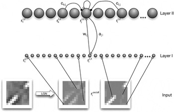
Our model consists of two layers, of which neurons are bidirectionally connected with each other by feedforward (W) and feedback (A) weights (Fig. 1). The activity  is obtained from images that have been whitened/lowpass filtered (see Materials and methods) and separated into ON–OFF channels (depending on the sign of the pixel value after filtering).
The network consists of two layers. The first layer (Layer I) represents the simulated input modulated by the “attentional” feedback signal (a). The cells of Layer II represent the simulated V1 cells. Each cell of Layer I gains feedback from all cells of Layer II (according to the feedback weight connection), and each Layer II cell obtains its main input from all Layer I cells [dependent on the feedforward weights (w), respectively, their receptive field]. This input is linear, but it is further processed nonlinearly. Each cell uses its current activation state to self-enhance its firing rate, but it is also inhibited by other cells, dependent on the current lateral inhibition connection weights (c).

Layer II gets activated from Layer I neurons but is dependent on the activity of other Layer II cells. The Layer II cells feedback to Layer I cells and increase their gain. Due to the learning of the feedback weights, this feedback is predictive. Unlike generative models where the difference between feedforward and feedback is computed, the feedback signal enhances the sensitivity of specific neurons in the previous layer and thus leads to an attentional tuning, as proposed by models of attention (Hamker, Reference Hamker2005).
Neural dynamics
We simulate the change in the firing rate of the cells with differential equations. The activity of model units is restricted to nonnegative values.
Layer I
The neurons in Layer I are driven by the ON- and OFF-cells (Fig. 1). Feedback from Layer II implements a gain modulation (Bayerl & Neumann, Reference Bayerl and Neumann2004; Hamker, Reference Hamker2004, Reference Hamker2005). There is no lateral competition among the neurons in Layer I, but they can receive a selective reentrant signal due to the competitive dynamics in Layer II. The firing rate  of Layer I cells is simulated by:

where

gives the gain enhancement via the feedback signal and

constrains the gain enhancement (Hamker, Reference Hamker2005).
i refers to the position of the neurons in the image space, τ L1 = 10 ms is the time constant of the temporal dynamics, aji denotes the feedback weight from neuron j of Layer II to neuron i of the first layer and (x)+ = max(x, 0).  and
 denote the strength of the firing rate for the corresponding neuron. The parameter A L1 = 1 determines the influence of the feedback signal with respect to the activity in the postsynaptic layer.
Layer II
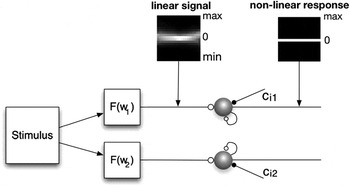
Layer II neurons learn a combination of specific input features. Their firing rates are determined by a linear input signal (the weighted sum of the activity in Layer I), nonlinear self-excitation, and nonlinear lateral inhibition to induce competition among cells (Fig. 2):

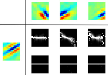
Each input stimulus is first processed linearly and forms the feedforward signal for the cells’ activation. The following processing modulates the firing rate nonlinearly due to self-excitation and lateral competition. The plot shows the change in the firing distribution along this processing using the average conditional histograms of all cell firing patterns. The nonlinear processing enforces the signal to be largely uncorrelated and independent.

where
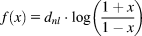
gives the nonlinear processing and

ensures that self-excitation saturates. The factor η = 2 determines the degree of self-excitation, and A L2 = 0.9 constrains the self-excitation. τ L2 = 10 is the time constant of the Layer II cells. The connection wij denotes the strength of the feedforward weight from neuron i of Layer I to neuron j of Layer II. Lateral inhibition can differ across the cells due to anti-Hebbian learning.
Learning rules
The learning of the connections between neurons is implemented via a Hebbian principle. Long-term potentiation requires an above-mean activation of both pre- and postsynaptic activities, which is well known as the covariance learning rule (Sejnowski, Reference Sejnowski1977; Willshaw & Dayan, Reference Willshaw and Dayan1990). Long-term depression occurs by the constraint to limit the overall weight resource and, only for the feedforward connections, if the presynaptic activity is below the population mean. Specifically, we used


 is the mean of the activation in a particular layer (e.g.,
 ) and τl = 5000 ms is the time constant for learning. The feedback weights are prevented from getting negative because the gain enhancing attentional signal is supposed to be only excitatory. αw = 3.5 and αa = 1.67 enforce a limitation of the weight resources. An appropriate value can be easily estimated from the stable solution of the ordinary differential equation (ODE) and the desired activation
 given
 .
Lateral connections within Layer II cells were learned by anti-Hebbian learning. The name anti-Hebbian implies that this strategy is the opposite of the Hebbian learning rule. Similar to the learning of the synaptic connection weights, where the connection between two cells is increased when both fire simultaneously, in the anti-Hebbian case the inhibition between two cells is strengthened. The more frequently two cells are activated at the same time, the stronger they inhibit each other, increasing the competition among the two cells:

where τc = 5000 ms is the learning rate of the anti-Hebbian weights. Anti-Hebbian learning leads to decorrelated responses and to a sparse code (Földiàk, Reference Földiàk1990). Falconbridge et al. (Reference Falconbridge, Stamps and Badcock2006) have shown that a model with anti-Hebbian learning of lateral weights develops Gabor-like receptive fields when trained with natural scenes. Our particular learning rule differs from the anti-Hebbian learning rule used by Földiàk (Reference Földiàk1990) and Falconbridge et al. (Reference Falconbridge, Stamps and Badcock2006). They used a fixed parameter (referring to a desired firing activity) to constrain the synaptic strength, while our constraint is dependent on the actual synaptic strength and the postsynaptic activity. Previous control simulations proved this anti-Hebbian learning rule to be superior in our framework.
Materials and methods
We applied the model to learn receptive fields from ON–OFF channel responses to natural scenes. In order to obtain the image data, we used the software package “nnscpack” from Patrik Hoyer (http://www.cs.helsinki.fi/u/phoyer/code/nnscpack.tar.gz), which in turn took the natural scenes from Bruno Olshausen’s “Sparsenet” software package (http://redwood.berkeley.edu/bruno/sparsenet). The image data consist of 10 images (512 × 512 pixels). To roughly simulate the characteristics of retinal ganglion cells, each image has been filtered with a zero-phase whitening/lowpass filter R(f) = f·exp(−(f/f 0)4) with f 0 = 200 cycles per picture (Olshausen & Field, Reference Olshausen and Field1996). This filter attenuates low frequencies and boosts high frequencies to obtain a roughly flat amplitude spectrum across spatial frequencies. In image space, this filter has a circularly symmetric, center-surround (Mexican hat) shape. For every image, the same number of randomly selected patches has been taken and used for learning. We did not define a training set with a fixed number of patches but randomly chose a patch for each trial. Each patch is divided in two different channels (ON–OFF), and each channel is normalized to unit mean-squared activation.
We used a 12 × 12 patch size. Thus, 288 cells were required in the first layer, that is, 144 neurons receive input from the ON- and the others from the OFF-cells. We used 288 cells in Layer II to represent the input combinations. The feedforward weights wij were initialized randomly with a mean  . The feedback and the lateral inhibition weights were initialized to zero. An image patch is presented for 50 ms to let the dynamics of the system converge to a stable state. After each trial, the feedback and feedforward synapses as well as the lateral inhibition connections are updated according to the final firing rates of the cells.
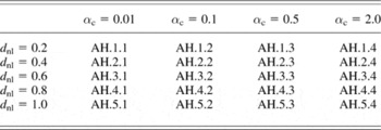
We controlled the competition in Layer II by two parameters, αc and dnl. The factor αc (eqn. 9) constrains the absolute strength of the anti-Hebbian weights. The factor dnl determines the degree of nonlinearity in the function f (see eqn. 5). Table 1 shows all combinations of parameters we used to modify the competition among the cells.
Parameters for the variation of competition

Twenty different parameter sets of our algorithm were tested, each with a different combination of the factor αc (controlling the strength of the anti-Hebbian weight connections) and d nl (controlling the nonlinear impact of the inhibition and the self-excitation). The parameter set AH.1.4 was excluded due to its bad performance.
Fitting the learned receptive fields to a Gabor-filter
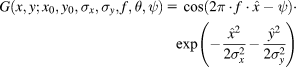
To compare the learned weight kernels or the receptive fields with Gabor functions, we estimated the parameters of the following equation using a nonlinear least-square data fitting approach:
with  and
 .
The parameters are as follows: x 0 and y 0 are the pixel coordinates of the Gabor-filter center, σx and σy refer to the width of the corresponding underlying Gaussian filters, f gives the frequency, θ gives the orientation, and ψ gives the phase of the Gabor-filter. The filter was fitted using a large-scale algorithm provided by MATLAB. This algorithm is a subspace trust-region method and is based on the interior-reflective Newton method described in Coleman and Li (Reference Coleman and Li1994, Reference Coleman and Li1996).
Efficient coding
Since efficient coding has been suggested to play a fundamental role in the principle of V1 processing, a good measure to evaluate this property must be found. To summarize, efficient coding means that an input stimulus is encoded with the least resources possible. Here we will introduce several measures, all capturing some aspects of the properties that constitute efficient coding. All measurements were calculated from Layer II cell responses to 50,000 randomly chosen image patches or combinations thereof. All following measurements for the efficiency of the codes (except sparseness) are best when they are small, thus for better clarity, the correlation with those measurements and the properties of the learned features are calculated with reversed axis.
Sparseness
The concept of sparse coding refers to a neural representation where only a few cells (out of a large population of cells) are effectively used to represent typical data vectors. There is strong theoretical evidence that natural scenes can be efficiently represented by a sparse code based on filters that resemble neurons found in area V1 (Barlow, Reference Barlow1989; Daugman, Reference Daugman1989; Field, Reference Field1984, Reference Field1994; Olshausen & Field, Reference Olshausen and Field1997). Sparse codes represent information with minimal redundancy and relatively few spikes. Regarding the cells’ metabolism and information processing, it is much more efficient than dense coding (Levy & Baxter, Reference Levy and Baxter1996; Laughlin et al., Reference Laughlin, de Ruyter van Steveninck and Anderson1998), where information is represented by the whole cell population. Vinje and Gallant (Reference Vinje and Gallant2000) argued that the shape of the receptive fields is responsible for forming a sparse code of the visual world and that the sparseness depends also on the size of presented natural image patches. However, evaluating sparseness in the activity of the brain is very difficult. Typically, the kurtosis of the firing distribution of the cells is used to measure the sparseness of the cell population. However, we decided to use the sparseness measure of a cell population r introduced by Hoyer (Reference Hoyer2004), which is gained from the following equation based on the relationship between the L 1 norm and the L 2 norm.

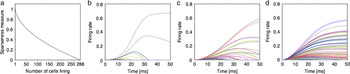
where r ∈ ℝn. The value is 1 if and only if r contains one single cell that is nonzero, and the value is 0 if all components respond equally (Fig. 3a). Fig. 3b–3d shows examples of cell populations’ responses with different sparseness values. The proposed measure shows the same tendency than using the kurtosis but is more gradual and due to its boundaries easier to compare.
(Color online) Illustration of sparseness. (a) The sparseness level is dependent on the number of active cells. On the x-axis, the number of active cells is plotted (for demonstration purposes, we used a binary code). The y-axis shows the corresponding sparseness value using eqn. (11). (b–d) The firing response for all Layer II cells to an image patch for three different trials with different lateral competition (and thus different levels of sparseness). According to this sparseness measure, the plotted examples had a sparseness of b: 0.9816, c: 0.8613, and d: 0.6758.

Correlation
Efficient coding means that the activation of neurons ought to be uncorrelated. The easiest way to measure correlation is to directly calculate the linear correlation between two neurons in response to multiple image patches.
Independence
In order to encode data even more efficiently, the neural responses ought to be independent from one another. This means that the information coding should make equal use of all possible combinations of activation patterns (Simoncelli & Olshausen, Reference Simoncelli and Olshausen2001). A statistical independence between two signals means that the knowledge of one signal provides no information about the other signal.
• Mutual information: To measure independence, it is common to consider the mutual information of the activation distributions. Mutual information of two variables can be understood as the amount of information that the knowledge of either variable provides about the other. Formally, the mutual information of two continuous random variables (X and Y) can be defined as follows:
(12)
where p(x, y) is the joint probability density function of X and Y, and p 1(x) and p 2(y) are the marginal probability density functions of X and Y, respectively. To assess the mutual information of a model, we estimated the mean mutual information between all possible responses of two cells using 50,000 image patches. Please refer to Kraskov et al. (Reference Kraskov, Stgbauer and Grassberger2004) for further details on the approximation of eqn. (12). This particular approximation has also been applied for the analysis of the natural statistics of optic flow generated on the retina during locomotion through natural environments (Calow & Lappe, Reference Calow and Lappe2007).
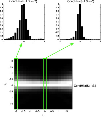
• Variance of the conditional distributions: Another way to examine independence is via a conditional histogram (Fig. 4); S 1 and S 2 refer to responses of two different Layer II cells to the 50,000 image patches. If the variance of the distribution of S 2 varies with the amplitude of S 1, then S 2 depends on S 1. No change in the variance across the distributions indicates independent signals. For each pair of neurons, we used the variance of the S 2 variances as a measure for the variance dependency. The mean of this variance over all cell combinations describes the degree of independent coding of a particular model.

(Color online) Average joint statistics of the response of linear filter pairs to randomly chosen natural image patches (results from model AH.1.2). Top: The response distribution of the filter S 2 subject to two different values of the filter S 1. Bottom: The two-dimensional conditional histogram as a gray-scale image. The intensity of the pixels is proportional to the bin counts with the exception that every column is rescaled to a maximum of 1. The upper histograms are slices of the conditional histogram. Different widths of these histograms indicate that the signals are not statistically independent.

Variance in the firing rate distributions
Willmore et al. (Reference Willmore, Watters and Tolhurst2000) argued that the variance of a cell’s firing rate to different stimuli is an indication of how “useful” this cell would be in the average coding process. A cell with high variance would respond much stronger and more frequent and thus having a greater impact encoding the stimuli.
• Variance-distribution: For an algorithm to code efficiently, Willmore et al. (Reference Willmore, Watters and Tolhurst2000) argued that it would mean that all cells are equally taking part in the coding process and thus, the cells ought to have a similar variance. To assess this, they introduced a so-called scree plot: The variance in the firing rate of each cell to different stimuli is computed, normalized, and then ordered in rank. They used the resulting plane as a measure of “dispersal.” An efficient code (with similar variance throughout all cells) would have a large plane (Willmore et al., Reference Willmore, Watters and Tolhurst2000). Another way to measure the dispersal is to take the gradient of the best linear fit. There, a small gradient would be expected in efficient codes (Watters, Reference Watters2004). We decided to use the gradient (further called the “Variance-distribution” measurement) because it is less delicate to outliers.
• Variance-mean: We also used a slightly different measurement to assess the property in how far each cell contributes to the overall coding in natural scenes. We looked at the variance of the average firing rate across all cells to the same image patches. The mean firing rate of each cell over the image patches is calculated, and the variance of all these means is used as the final measurement. The smaller the variance, the more similar is the average firing rate across all cells. This measure (further called “Variance-mean” measurement) gives information about the probability of the cells’ firing with the same strength on average. This might sound very similar to the Variance-distribution measurement, but we will show later that those two values do capture different aspects.
Properties of V1 receptive fields
The data from Ringach et al. (Reference Ringach, Bredfeldt, Shapley and Hawken2002) were used as a ground truth of V1 receptive field properties. In this study, the cells of the macaques were stimulated by drifting sinusoidal gratings, and a spatiotemporal receptive field of simple cells was measured using subspace reverse correlation. For a comparison to these data, we only considered receptive fields from our models that were adequately fitted by Gabor-filters (i.e., sum-of-squares difference <3). To assess the receptive field properties, we determined the following two measurements:
• Average frequency: We took the average frequency of the Gabor-fitted receptive fields to roughly describe the frequency tuning of the receptive fields.
• Fit to the macaque data: To directly compare the results of our algorithm with the electrophysiological data, we determined the average distance of each data point from the macaque data to its nearest corresponding data point of the model data and vice versa. A small average distance would therefore indicate that the learned receptive fields match the macaque data well.
Coding quality
To assess the quality of coding, we used two different measurements:
• Reconstruction of the original image: As the cell responses are coding the input image patches according to the learned feedforward matrices, we assessed the quality of this code by comparing the linear reconstruction of the image with the original image patch in a least square manner. Our models do not optimize their weights to reduce the error between the original and the reconstructed image but learn correlations between the input and nonlinear responses, thus we had to estimate how our model would reconstruct the image. The reconstructed image is estimated as follows:
(13)where
is the vector of the nonlinear ON-cell responses to the original image patch I and Won the corresponding weights to the ON-cells ( and Woff, respectively). To capture the amount of reconstructed information correctly, we normalized the constructed image to the same mean as I before calculating the image reconstruction error. As the weights W and A mostly learn the same correlations, the reconstructed image is nearly identical when using W compared to A after normalization. The smaller the reconstruction error, the better is the algorithm. The correlation between this measurement and efficient coding measurements is therefore calculated with a reversed axis.• Similarity of the cell populations: Object recognition requires to discriminate between different population responses. At the level of V1, a simple measure of the discrimination ability is to assess the similarity of the population responses (r and s) to two randomly chosen image patches by computing the angle between the vectors:
(14)with
. The statistical probability for overlapping cell responses increases with the number of active cells, thus, the sparser the population codes, the higher is the bias for a good discrimination. In order to diminish this effect, we normalized each discrimination value with the expected discrimination given the corresponding distribution of firing rates. For each model, we created 100,000 pairs of random cell responses according to the distribution of the firing rates and calculated their discrimination to obtain the expected discrimination.

 is the vector of the nonlinear ON-cell responses to the original image patch I and Won the corresponding weights to the ON-cells (
 and Woff, respectively). To capture the amount of reconstructed information correctly, we normalized the constructed image to the same mean as I before calculating the image reconstruction error. As the weights W and A mostly learn the same correlations, the reconstructed image is nearly identical when using W compared to A after normalization. The smaller the reconstruction error, the better is the algorithm. The correlation between this measurement and efficient coding measurements is therefore calculated with a reversed axis.
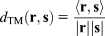
 . The statistical probability for overlapping cell responses increases with the number of active cells, thus, the sparser the population codes, the higher is the bias for a good discrimination. In order to diminish this effect, we normalized each discrimination value with the expected discrimination given the corresponding distribution of firing rates. For each model, we created 100,000 pairs of random cell responses according to the distribution of the firing rates and calculated their discrimination to obtain the expected discrimination.
Results
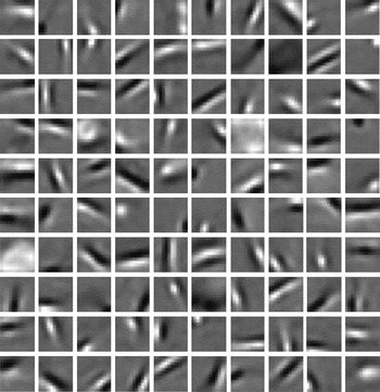
Fig. 5 shows the learned weight kernels for our algorithm with a particular set of parameters (AH.5.1) after 400,000 image patch presentations. Although the shapes of the weight connections are visible after about 30,000–100,000 presentations (dependent on the algorithm parameters), the detailed learned “feature” can vary over time due to the lateral inhibition. The bottom-up and top-down weights converged to similar profiles (median of the sum-of-squares differences for the models vary from 0.067 to 0.343). In all parameter sets of our algorithm, most of the kernels are localized, oriented, and band-pass, similar to several earlier approaches. We also obtain blob-like kernels which appear absent in the classical sparse coding model (Olshausen & Field, Reference Olshausen and Field1996) and in ICA (Bell & Sejnowski, Reference Bell and Sejnowski1997; van Hateren & van der Schaaf, Reference van Hateren and van der Schaaf1998).
100 randomly chosen feedforward weights of the parameter set AH.5.1 (Table 1) after learning for 400,000 trials. Pixels brighter than gray indicate excitatory and darker than gray indicate inhibitory weight connections. The weights often converge to localized, oriented band-pass filters.

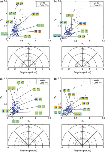
To estimate the receptive field profile, including the whitening/lowpass filtering stage, we convolved the whitening/lowpass filter with the learned weights, which basically slightly reduces the frequency but does not change the overall shape. The receptive fields are well fitted with Gabor functions. In our algorithm with a particular parameter set leading to the receptive field kernels shown in Fig. 5 (AH.5.1), the median of the sum-of-squares difference is 1.93 (with 0.9-Quantile = 6.05 and 0.1-Quantile = 0.60). The resulting receptive fields using other parameter sets are similarly well fitted. However, there are large differences in the properties of the weight kernels across the parameter sets of our algorithm (Fig. 6). In the following, we systematically compared the model receptive field properties with V1 data with respect to measures of efficient coding (see Materials and methods). The parameter set AH.1.4 is excluded from further evaluation due to its extraordinary weak fit.
(Color online) The properties of the Gabor-fitted receptive fields of the model for four different parameter sets. (a) Model with the lowest nonlinearity and a high constraint of the inhibition weights (AH.1.3). (b) Model with the lowest nonlinearity and the lowest inhibition constraint (AH.1.1). (c) Model with the highest nonlinearity and the lowest inhibition constraint (AH.5.1). This model shows the highest sparseness. (d) Model with the highest nonlinearity and the highest inhibition constraint (AH.5.4). The upper panels show the distribution of the dimensional preference of the fitted Gabor-filters model data in blue and electrophysiological data by Ringach et al. (Reference Ringach, Bredfeldt, Shapley and Hawken2002) in gray. The vertical dimension ny refers to the product of frequency and σ of the underlying Gaussian in the vertical direction (f·σy) and the horizontal dimension accordingly nx = f·σx. The lower panels show the distribution of the frequency of the fitted Gabor-filters with respect to their orientation. The results of those models are as follows: average frequency: (a) 1.07, (b) 0.80, (c) 1.11, and (d) 0.93; and distance to the biological data plot: (a) 0.054, (b) 0.095, (c) 0.051, and (d) 0.082.

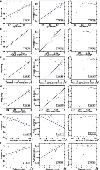
As we affected the inhibition among the Layer II cells, the resulting instances show different levels of sparseness. The range of sparseness reaches from 0.72 up to 0.92 across the parameter sets (for comparison, the kurtosis values vary between 21 and 196). Fig. 7a shows the correlation between the average sparseness of the models and the properties of the learned receptive fields, that is, the median frequency (F), the difference between model and data (Diff), and the reconstruction error (RC). All these three measures show a strong correlation with sparseness (rF = 0.91, r Diff = 0.94, and r RC = 0.63). In other words, with increasing sparseness of the Layer II cell population, the properties of the model receptive fields become more similar to the V1 data. Note that the image reconstruction error saturates and slightly drops with increasing levels of sparseness.
(Color online) Correlation between efficient code measurements and receptive field properties. The efficient code measurements of our algorithm (abscissa) are plotted against the different properties (ordinates) of the algorithm. The average frequency of the receptive fields, the difference to the electrophysiological data, and the image reconstruction error. The blue lines are the best linear fit in a least squared error manner. (a) Sparseness strongly correlates with the similarity between the model and the biological data. The image reconstruction error decreases with stronger sparseness. (b) Mutual information is similarly strong correlated, and the reconstruction error saturates with low levels of mutual information. (c) The variance of the conditional distributions is more weakly correlated. (d) The linear correlation of the cell responses shows a similar profile as sparseness and mutual information. (e) The Variance-distribution measurement shows a completely opposite correlation as expected. With a “better” Variance-distribution measurement, the similarity between model and biological data decreases. There is no correlation with the reconstruction error. (f) The Variance-mean measurement only shows a very low correlation with the similarity between model and biological data and no correlation at all with the reconstruction error.

The average mutual information of the Layer II responses shows a similar correlation with the receptive field properties (rF = 0.94, r Diff = 0.92, and r RC = 0.72) as sparseness (Fig. 7b).
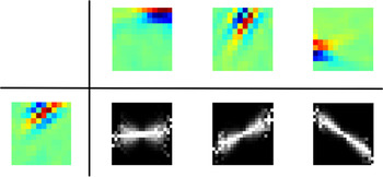
The conditional histograms contain information about the independence and the correlation of the corresponding cell responses. Fig. 8 shows examples of the average conditional histogram of the linear part and the nonlinear response of the particular parameter set shown in Fig. 6c (AH.5.1). The nonlinear stage effectively removes the redundancy in the linear responses. Since this effect is found in all parameter sets of our algorithm, the variance of the conditional distributions is always very low but a bit noisy and therefore, the correlation between the variance of the conditional distributions and the properties of the receptive fields is much smaller compared to the mutual information and sparseness (rF = 0.47, r Diff = 0.41, and r RC = 0.60) (Fig. 7c).
(Color online) Conditional distribution examples (AH.5.1). The conditional distribution of the linear part of our algorithm and the nonlinear response is shown for three different pairs of cells. While the linear part of the cell responses shows a dependency and a correlation, the nonlinear responses are often completely decorrelated and independent as shown in this example.

The linear correlation among the cell responses (Fig. 7d) shows a strong correlation similar to sparseness and mutual information (rF = 0.95, r Diff = 0.88, and r RC = 0.80).
Until now, we have only considered the properties of the cell population codes in terms of sparseness, dependency, and correlation. As described earlier, efficient coding can also be defined such that each cell participates to a similar degree in the probability of encoding natural scenes. Fig. 7e shows the results of the Variance-distribution measurement proposed by Watters (Reference Watters2004). The correlations are opposite to the results one would have expected. Following the lead of the previous measurements of efficient coding, one would expect that if the gradient of the fitted linear function becomes more flat (and thus the variance in the firing rates would become similar), the similarity of the model with the V1 data increases. Obviously, the correlation points in the opposite direction (rF = −0.71, r Diff = −0.72, and r RC = −0.34). Thus, the similarity of model and data is not increased with a more similar variance in the firing rates across all cells. To complement this observation, we also tested the linear part of the firing rates. The correlation for the linear part also shows negative correlations.
If we use the mean-distribution as a measurement of the contribution of each cell to the neural code, we find a weak correlation (rF = 0.48, r Diff = 0.71, and r RC = 0.25). Thus, with similar mean firing rates across the cells, the properties of the model receptive fields become more similar to the V1 data (Fig. 7f). The image reconstruction error does hardly correlate with the variance of the average firing rates.
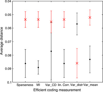
The influence of the different efficient coding estimates can be seen in Fig. 9. For each estimate, the best and worst five methods were picked out, and the average difference of the model to the V1 data is plotted. For all estimates of efficient coding (except the Variance-distribution measurement), the parameter sets that best implement efficient coding lead to a better fit of the model with V1 data. Only the Variance-distribution measurement shows complete converse results. Thus, equal variance of the cell responses appears not to be a good measurement for efficient coding since it does not only deviate from other estimates, but achieving a more equal variance results in a weaker fit to the data.
(Color online) For all efficient coding measurements, the best five (red cross) and the worst five (black dots) models were evaluated with respect to the average distance of the model data to the electrophysiological data. Note that the outlying model (AH.1.4) was excluded in this analysis. On the y-axis, the difference to the data is plotted. The bars refer to the standard deviation of the corresponding five averaged models. All measurements (except the Variance-distribution measurement) show the same effect, that the models with a more efficient code (according to the measurement) also fit the macaque data better. Sparseness = sparseness measurement; MI = mutual information; Var_CD = variance of the conditional distributions; linCorr = linear correlation; Var_distr = Variance-distribution measurement; and Var_mean = Variance-mean measurements.

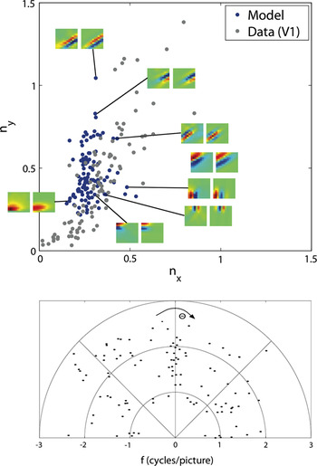
We now compare our results to ICA, a standard linear method for learning receptive fields from natural scenes. Here, we use the fast fix-point algorithm (Hyvärinen et al., Reference Hyvärinen, Karhunen and Oja2001). Hoyer and Hyvärinen (Reference Hoyer and Hyvärinen2000) have shown that this algorithm can produce orientated band-pass filters similar to those in V1. Fig. 10 shows the results of their algorithm applied to the same natural scenes we used for our algorithm. The results show similar deficits than the results from Lewicki et al. (Reference Lewicki, Hughes and Olshausen1999) and more mild deficits compared to those Ringach et al. (Reference Ringach, Bredfeldt, Shapley and Hawken2002) have shown for Bell and Sejnowski’s (Reference Bell and Sejnowski1997) ICA and the Olshausen and Field (Reference Olshausen and Field1996) sparse coding algorithm. ICA does not show receptive fields near the origin.
(Color online) The properties of the Gabor-fitted receptive fields obtained by the ICA algorithm. The upper panel shows the distribution of the dimensional preference of the fitted Gabor-filters model data in blue and electrophysiological data by Ringach et al. (Reference Ringach, Bredfeldt, Shapley and Hawken2002) in gray. The vertical dimension ny refers to the product of frequency and σ of the underlying Gaussian in the vertical direction (f·σy) and the horizontal dimension accordingly nx = f·σx. The lower panel shows the distribution of the frequency of the fitted Gabor-filters with respect to their orientation. Note that small frequencies and thus data points near the origin are completely missing.

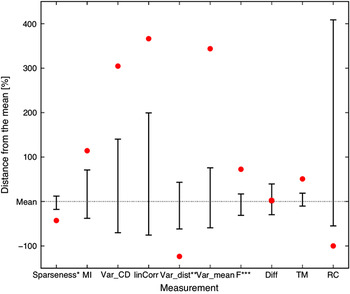
We evaluated the ICA results in terms of efficient coding and properties of the learned receptive fields and population codes. Fig. 11 shows those results in direct comparison to our results. Nearly all measurements for the efficiency of the code show weaker values compared to our algorithm across all parameter variations. The ICA code is much less sparse than our algorithm, the same holds for the mutual information which is much higher, the variance of the conditional distributions and the Variance-mean measurement where the ICA algorithm shows much higher values and thus a weaker efficiency of the code. The variances in the responses are also less equal to each other across the neurons although this measurement does not predict a similarity to biological data in our algorithm. Looking at the properties of the receptive fields, the ICA algorithm shows a higher average frequency. The distance to the electrophysiological monkey data is near the mean performance of the parameter sets of our algorithm but worse than the results from the better parameter sets. The population responses of the ICA algorithm are much more similar across different patches as compared to our algorithm whereas the reconstruction error of the ICA is negligible, as expected since the ICA tunes the weights to minimize the difference between the input and reconstructed image.
(Color online) The results of the ICA in comparison to the parameter sets of our algorithm. The dotted line indicates the mean of the measurements over all parameter sets. The upper, respectively, lower error bar indicates the parameter sets with the highest, respectively, the lowest distance to the mean. The red dots show the results of the ICA algorithm also with respect to the mean of our algorithm. The lower the value, the better the result. (§This measurement is better with higher values; §§since the mean of our algorithm is negative, values above the mean indicate a better performance; §§§the frequency is better when higher in average but too high values are not plausible compared to electrophysiological data.) Sparseness = sparseness measurement; MI = mutual information; Var_CD = variance of the conditional distributions; linCorr = linear correlation; Var_distr = Variance-distribution measurement; Var_mean = Variance-mean measurement; F = frequency; Diff = difference of the data plot to the electrophysiological data; TM = template match; and RC = image reconstruction error.

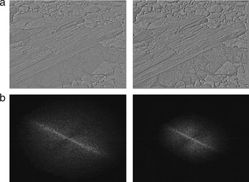
To visualize the image reconstruction performance in our model, we reconstructed one of the images that was used during the learning process with the receptive fields weighted by the firing rates of the corresponding cells (Fig. 12). The reconstructed image is close to the original but with slight impairments. The corresponding frequency planes show that the reconstructed image misses particular higher frequencies and thus smaller details.
Linear reconstruction of the image. The image was divided in 63 × 63 image patches, and the Layer II responses for each of these patches were computed. An image patch was then reconstructed by summing all 288 filters (weighted by their corresponding Layer II cell activation). The whole reconstructed image consists of the reconstructed image patches (averaged when overlapping). (a) Left: The original input image (whitened). Right: The reconstructed image. The reconstructed image shows the same features as the original image, but it appears slightly blurred. (b) The Fourier transformations of the corresponding images. The low frequencies are located in the center of the image. The reconstructed image misses higher frequencies.

Discussion
It has been proposed that efficient coding is one of the goals of sensory processing in the brain (Attneave, Reference Attneave1954; Barlow, Reference Barlow and Rosenblith1961). According to that, most models have been created to optimize the efficiency using an objective function. The basic idea is that there exists an “optimal” state, and the algorithms try to minimize the difference between the actual network state and this optimal state. Using this approach, Olshausen and Field (Reference Olshausen and Field1997) were one of the first to show that by enforcing a certain level of sparseness, their algorithm was able to learn oriented, Gabor-like filters. However, Ringach et al. (Reference Ringach, Bredfeldt, Shapley and Hawken2002) have shown that the results of Sparsenet as well as typical ICA learned filters do not fit well with the whole population of V1 macaque data. Those models were only able to capture a part of the variety of V1 receptive fields, and lower frequencies were completely missing. Since then, some researchers tried to overcome the limitations the early generative models showed. Recently, Rehn and Sommer (Reference Rehn and Sommer2007) as well as Weber and Triesch (Reference Weber and Triesch2008) introduced models that converge to receptive fields more similar to those of V1. Rehn and Sommer (Reference Rehn and Sommer2007) used a hard-sparseness model which optimizes the sparse selection of active neurons. Compared to a soft-sparseness example algorithm, namely the Sparsenet model of Olshausen and Field (Reference Olshausen and Field1996), the competition among cells now involves nonlinear operations, a threshold function, and multiplicative gating. Weber and Triesch (Reference Weber and Triesch2008) have expanded the generative approach with a nonlinear output function. The output activity is rescaled according to a sigmoid function. The transfer function depends on certain parameters that are adjusted to keep the neural output of each neuron in an approximately exponential regime. Nevertheless, these algorithms still show some weaknesses. The algorithm of Rehn and Sommer (Reference Rehn and Sommer2007) leads to filters with a blob-like shape, but inconsistent with the macaque data, there is a gap between filters near the origin and those further out. Similarly, the model of Weber and Triesch (Reference Weber and Triesch2008) leads to filters near the origin, but the distribution close to the origin differs from the macaque data. Additionally, both models show several filters in the middle frequency range that have also not been observed in the electrophysiological data. However, both models show more filters with higher frequencies than our model. The model of Weber and Triesch (Reference Weber and Triesch2008) might potentially overrepresent the higher frequencies, but clearly our model sightly underrepresents higher frequencies. The underrepresentation of higher frequencies could have several reasons. One might be the local definition of Hebbian learning. Each output unit produces its own “reconstructed” image. A generative model, however, uses an objective function to minimize the error between the original image and the reconstructed image, that is, the sum of all units. This function enforces a global reconstruction of the image, which is not enforced by local Hebbian learning. Thus, without this enforcement, higher frequencies that are less common in the image than lower frequencies (Fig. 12) are less likely to be learned. The underrepresentation of higher frequencies could have been compensated by emphasizing higher frequencies in the filtering of the input image (LGN model), but to compare our data to other models, we decided to use identical parameters as in Olshausen and Field (Reference Olshausen and Field1996). Concluding, the macaque data obtained by Ringach et al. (Reference Ringach, Bredfeldt, Shapley and Hawken2002) were very well fitted by a Hebbian/anti-Hebbian learning principle with a nonlinear neural dynamic.
So far, we have compared our model to others with respect to experimental data. We now discuss how our approach relates to the efficient coding hypothesis. The common procedure to investigate efficient coding is by means of an objective function that, if optimized, allows to reveal insights about the underlying principles of coding by comparing the result to data. We here take a different approach to investigate efficient coding. Instead of optimizing a particular objective function, we have designed a simple V1 model composed of biologically plausible elements. We measure coding efficiency in this model while changing critical model parameters and relate this measure to the similarity between model and experimentally obtained receptive field data. Our model strongly relies on lateral inhibitory connections as determined by anti-Hebbian learning. A recent study emphasized the importance of lateral inhibitory connections. Ren et al. (Reference Ren, Yoshimura, Takada, Horibe and Komatsu2007) observed in layer-2/3 of the mouse visual cortex axo-axonic inhibition to nearby pyramidal cells bypassing the classical route via inhibitory interneurons. Schwartz and Simoncelli (Reference Schwartz and Simoncelli2001) have also shown that lateral inhibition can improve the coding efficiency regarding the independence of the neural responses. We have identified parameters of our model (namely the lateral competition among the Layer II cells) that allow us to control the level of efficiency.
We have recently proposed a similar Hebbian learning model that learns Gabor-like receptive fields even with a less sparse distribution of the output firing rate (Hamker & Wiltschut, Reference Hamker and Wiltschut2007). This model relied on presynaptic inhibition to decorrelate the responses, where the lateral weights are not independently learned but determined by the feedforward weights. However, presynaptic inhibition implements only a weak competition and thus leading to output activations that are not very sparse. The anti-Hebbian approach proposed here more effectively decorrelates the neural responses compared to presynaptic inhibition and leads to a significantly improved fit to V1 data.
Falconbridge et al. (Reference Falconbridge, Stamps and Badcock2006) have modified the Hebbian/anti-Hebbian model of Földiàk (Reference Földiàk1990) with a nonlinear function that reflects biological data more closely, but the model does not capture the full range of the distribution. In particular, they missed the low frequency range almost completely. Their Hebbian learning rule is very similar to the original learning rule of Oja (Reference Oja1982); our learning rules (eqns. 7 and 8), on the other hand, are covariance learning rules (i.e., adapting the firing rates according to the corresponding population means). Their output activation is directly modified by a nonlinear function, whereas the nonlinearity in our model only regulates the lateral competition. Our model always produces low-frequency Gabor-filters, and only with an increase in the efficiency of the codes, also higher frequencies can be obtained. This allows the assumption that nonlinear competition is particularly effective for learning biologically plausible receptive fields from natural scenes.
With increasing competition (respectively with increasing sparseness of the Layer II cell populations), the properties of the algorithm become closer to the electrophysiological macaque data. Other efficient coding properties like independence, as estimated by mutual information or the linear correlation of the cell responses, lead to the same result, namely an increase in the similarity of the receptive fields to V1 data. However, the correlations using the variance of the conditional distributions and the variance across the mean firing rate are lower than the one with sparseness or mutual information. While for the chosen parameters the model converges always to relatively similar receptive fields, a too weak competition impairs convergence (e.g., AH.1.4 showed such a bad performance that we excluded it from further evaluation). The goal to achieve an equal variance across all cell responses as a measure of efficient coding does not correlate with the similarity of model and experimental data. Thus, equal variance appears as a problematic measurement of efficient coding.
We have shown not only that the properties of the receptive fields do depend on measurements of efficient coding but also that the similarity of the model data with the V1 macaque data increases with higher efficiency. Models with higher sparseness show a higher average frequency of the receptive fields and a better fit to the macaque data compared to those with low sparseness (e.g., cf. Fig. 6). As far as the coding quality is concerned, we found that models whose codes are too sparse, too independent, or too decorrelated show a decrease in image reconstruction. However, image reconstruction might not be the ultimate goal of vision. Visual perception is probably more concerned with object discrimination. Thus, the quality of a code lies rather in the ability to be further processed by higher order modules that need to discriminate one population from one another. The ICA algorithm is laid out to reconstruct the original information perfectly, whereas our algorithm shows a weaker image reconstruction but leads to code vectors that are much better discriminable. This result appears somewhat surprising. Although the ICA allows for a perfect reconstruction, the code vectors associated with different image patches are much more similar to each other (in terms of the normalized angle between the vectors) than as observed in our model. Of course, the reconstruction ability demonstrates that all information is encoded in the ICA code vectors, but the usefulness of ICA for pattern discrimination critically depends if this information can be used in later stages.
As has been pointed out earlier, linear ICA does not ensure that the resulting codes are largely independent and decorrelated (Karklin & Lewicki, Reference Karklin and Lewicki2003; Bethge, Reference Bethge2006), see also Fig. 13. If independence ought to be a guiding principle of efficient coding for vision, linear ICA is probably not the ideal solution. Schwartz and Simoncelli (Reference Schwartz and Simoncelli2001) provided evidence that nonlinear lateral inhibition for gain normalization eliminates a number of dependencies. We have shown that this concept can be generalized to an anti-Hebbian learning of lateral weights. Our code vectors are largely decorrelated and independent (cf. Fig. 8).
(Color online) Conditional distribution examples of the ICA algorithm. The examples show that the ICA algorithm leads to some pairs of cell responses that are dependent on one another and even sometimes correlated.

We conclude that Hebbian/anti-Hebbian learning is consistent with the framework of efficient coding. Particularly, nonlinear lateral interactions lead to more independence which also increases the similarity between the model and experimental data. Too strong lateral inhibitory connections, however, impair the coding quality.
Acknowledgments
This work has been supported by the German Research Foundation (Deutsche Forschungsgemeinschaft) grant “A neurocomputational systems approach to modeling the cognitive guidance of attention and object/category recognition” (DFG HA2630/4-1) and by the European Union grant “Eyeshots: Heterogeneous 3-D Perception across Visual Fragments.”