

1. INTRODUCTION
Over the past few years we have developed a velocity dependent Krook (VDK) model (Manheimer et al., Reference Goncharov, Sangster, Radha, Betti, Boehly, Collins, Craxton, Delettrez, Epstein, Glebov, Hu, Igumenshchev, Knauer, Loucks, Marozas, Marshall, McCrory, McKenty, Meyerhoffer, Regan, Seka, Skupsky, Smalyuk, Sources, Stoeckl, Shvarts, Frenje, Petrasso, Li, Seguin, Manheimer and Colombant2008; Colombant & Manheimer, Reference Colombant and Manheimer2008; Reference Colombant and Manheimer2009; Reference Colombant and Manheimer2010a; Reference Colombant and Manheimer2010b; Manheimer et al., Reference Manheimer, Colombant and Schmitt2012) to study nonlocal transport in laser produced plasmas. Other authors have developed similar models (Goncharov et al, Reference Goncharov, Gotchev, Vianello, Boehly, Knauer, McKenty, Radha, Regan, Sangster, Skupsky, Smalyuk, Betti, Mc Croyy, Meyerhoffer and Cherfils-Clorouin2006; Reference Goncharov, Sangster, Radha, Betti, Boehly, Collins, Craxton, Delettrez, Epstein, Glebov, Hu, Igumenshchev, Knauer, Loucks, Marozas, Marshall, McCrory, McKenty, Meyerhoffer, Regan, Seka, Skupsky, Smalyuk, Sources, Stoeckl, Shvarts, Frenje, Petrasso, Li, Seguin, Manheimer and Colombant2008; Schurtz et al., Reference Schurtz, Nicolai and Busquet2000). One common feature to all models as opposed to earlier models based on convolution of the Spitzer conductivity with some kernel (a full discussion of these can be found in Manheimer et al. (Reference Goncharov, Sangster, Radha, Betti, Boehly, Collins, Craxton, Delettrez, Epstein, Glebov, Hu, Igumenshchev, Knauer, Loucks, Marozas, Marshall, McCrory, McKenty, Meyerhoffer, Regan, Seka, Skupsky, Smalyuk, Sources, Stoeckl, Shvarts, Frenje, Petrasso, Li, Seguin, Manheimer and Colombant2008), is that these more recent models break up the velocity space into a low energy part that is treated locally, and a high energy part that is treated nonlocally.
The problem of nonlocal transport in laser produced plasmas is actually made up of three problems that we briefly discuss separately now. First there is the case of plasma in which most electrons have a mean free path short compared to relevant gradients, but for which the energetic electrons, which transport the energy, have a mean free path that could be longer than the gradient scale length. This case is characterized by a nonlocal tail on the electron distribution function. Generally, the energy here is a few tens of keV. This is the case studied in Goncharov et al. (Reference Goncharov, Gotchev, Vianello, Boehly, Knauer, McKenty, Radha, Regan, Sangster, Skupsky, Smalyuk, Betti, Mc Croyy, Meyerhoffer and Cherfils-Clorouin2006; Reference Goncharov, Sangster, Radha, Betti, Boehly, Collins, Craxton, Delettrez, Epstein, Glebov, Hu, Igumenshchev, Knauer, Loucks, Marozas, Marshall, McCrory, McKenty, Meyerhoffer, Regan, Seka, Skupsky, Smalyuk, Sources, Stoeckl, Shvarts, Frenje, Petrasso, Li, Seguin, Manheimer and Colombant2008); Colombant and Manheimer (Reference Colombant and Manheimer2008; Reference Colombant and Manheimer2009; Reference Colombant and Manheimer2010a; Reference Colombant and Manheimer2010b), Manheimer et al. (Reference Manheimer, Colombant and Schmitt2012), and Schurtz et al. (Reference Schurtz, Nicolai and Busquet2000). We call this case a nonlocal tail.
Second, such plasma could be subject to a variety of laser plasma instabilities, such as the two plasmon decay (TPD) instability, which produces a separate spectrum of energetic electrons at, for instance, the quarter critical surface. This case has an energetic tail on the distribution function. Generally, the tail energies are much higher than the nonlocal tail; they range from perhaps one hundred to several hundred keV. These electrons are produced at a particular point in space and move into the target plasma and deposit their energy inside. A particular worry about these is that in a laser fusion situation, they may preheat the core, prematurely raise its adiabat and prevent full compression of the fuel. As such, it is important that the behavior of these electrons, once they are produced, be analyzed as carefully as possible. This is the goal of this paper. Here we apply our VDK model, which we have applied to the nonlocal tail and to the energetic tail. As we will see, there are similarities and differences in the way the theory is applied to the two different situations. There are other approaches to this problem that we discuss in the next section. However, little has appeared in the archival literature over the years. We call this case an energetic tail.
Finally, there is a super energetic population of electrons that might be produced by a powerful femto-second laser to get fast ignition (Hou et al. Reference Hou, Wu, Cal, Chen, Lao, Wang and Chew2010; Honrubia et al., Reference Honrubia, Antonicci and Moreno2004; Alouanibibi et al., Reference Alouanibibi, Matte and Kieffer2004). These are megavolt and multi-megavolt electrons, are fully relativistic, and are generally studied by particle in cell (PIC) simulations. We call this case a super energetic tail. In this paper we treat only the case of the energetic tail.
2. THE STATE OF THE ART
It is not easy to discern how energetic electrons are handled in fluid simulations of laser produced plasmas. There is a vast literature on how they might be produced by plasma instability, most likely the TPD instability for the case of direct drive laser fusion. But less has been published on how fluid simulations handle the transport of these electrons. There appear to be four methods used in the literature; multi-group flux limited diffusion as used in LASNEX, Fokker Planck simulations, PIC simulations of the TPD, and simple deposition models. Here we briefly discuss each.
There have been at least two textbooks (Kruer, Reference Kruer1988; Lindl, Reference Lindl1998) written by laser fusion scientists at the Lawrence Livermore National Laboratory (LLNL), and each has a chapter on the effect of energetic electrons. However, despite the number of references in these chapters, only two are usable for the problem at hand. Kruer (Reference Kruer1988) cites a Comment, which outlines the approach used in the fluid simulation LASNEX (Zimmerman & Kruer, Reference Zimmerman and Kruer1975). Lindl (Reference Lindl1998) cites one treatise by Rosen et al. (Reference Rosen, Price, Campbell, Phillion, Estabrook, Lasinski, Auerbach, Obenschain, McLean, Whitlock and Ripin1987), but says it is unavailable, and cites another paper, which uses a simple deposition model.
Input to their flux limited multi-group diffusion model (Zimmerman & Kruer, Reference Zimmerman and Kruer1975) consists of an assumed temperature of the hot electron temperature and the fraction of laser energy put into hot electrons as opposed to thermals. Presumably, knowledge of the laser plasma instability provides this. Typically, they assume a hot temperature of 12 times the thermal temperature, and in their paper they do not appear to specify the fraction of laser energy going into the hot electrons as opposed to the thermal. This specification of energetic component is necessary for any model, and is in a sense equivalent to the assumptions we make here about the distribution function of energetic electrons at the quarter critical surface where the TPD instability occurs. The LLNL Inertial Fusion Annual and Semi Annual reports from 1996 onward are on the LLNL website, and occasionally they discuss this. For instance, Harte et al. (Reference Harte, Alley, Bailey, Eddleman and Zimmerman1998) discussed this, but provided even fewer details than Zimmerman and Kruer (Reference Zimmerman and Kruer1975).
Their theory appears to be based on two old LLNL reports (Zimmerman, Reference Zimmerman1973; Kershaw, Reference Kershaw1979), which are not widely available. The hot electron component is broken up into energy bins, and each bin has a velocity (actually current) given in Zimmerman and Kruer (Reference Zimmerman and Kruer1975) and Zimmerman (Reference Zimmerman1973). Since they used a diffusion model, this current is proportional to pressure gradient of each energy component and the conductivity times the electric field. They justify a diffusion model by assuming the energetic electron distribution is nearly isotropic. This is based on their assumption that the ion charge Z is large, and in regions where Z ~ 1, they assume the energetic electrons are isotropic because of a strong magnetic field. However, in the laser fusion targets, most of the plasma has Z ~ 1, and in spherical plasma it is not clear that there would be strong magnetic field at all. Furthermore, the magnetic field gives isotropy only in the two directions perpendicular to it, and in the simplest theory, does so only for straight field lines.
To keep the flux from getting very large due to the high conductivity of the energetic electron group, they used a flux limit. It is difficult to see what their flux limit is from their published work, but it appears to be the density of the quantity being convected times the velocity of the electron at that particular energy. This is most clearly spelled out by Kershaw (Reference Kershaw1979). However, the flux limit is obviously a parameter that they specify to do the calculation. For the case of thermal electron transport, a flux limit has often been used, and there have been many estimates for it. However, in nearly all cases, the limiting velocity, for the thermal electron transport case, has been chosen to be much less than the electron thermal velocity.
Zimmerman and Kruer (Reference Zimmerman and Kruer1975) give the electric field from a zero current condition, accounting for both the thermal and energetic electrons. Also there are energy exchanges between the groups, which they estimate based on the Fokker Planck expression for the slowing down and diffusion of energetic electrons in velocity space. These energetic electrons also heat the thermal electrons. The equations they solve are specified in detail (Zimmerman, Reference Zimmerman1973, Appendix II). The energetic electron equation is solved in the time domain, but is solved implicitly. While this model has undoubtedly changed and evolved over the last 40 years, LLNL does not seem to have documented these advances.
Any independent group attempting to confirm LLNL's results using their model would have a difficult time going to the literature and finding out just what to do. There seem to be many choices one can make in the model, even assuming that it is still used as it was in 1974. These include choices of initial bin assignment, flux limit, fraction of energy going to the energetic species, temperature (they usually assume 12 T, but apparently they also did some calculations with an assumed temperature of 6 T). These do not seem to have been specified by the LLNL group in their reports of results. However, the multi-group flux limited diffusion approach does seem to be compatible with fluid simulations of laser plasma implosions; likely it fits in well with the code infrastructure used for radiation transport.
Another approach developed by a variety of groups is the use of a Fokker Planck simulation (Nishigushi et al., Reference Nishigushi, Mima, Azechi, Miyanaga and Nakai1992; Honda et al., Reference Honda, Nishiguchi, Takabe, Azechi and Mima1996; Sunahara et al., Reference Sunahara, Delettrez, Stoeckl, Short and Skupsky2003; Epperlein, Reference Epperlein1994; Alouanibibi & Matte, Reference Alouanibibi and Matte2007; Keshinen & Schmitt, Reference Keskinen and Schmitt2007). The fluid ions are treated in the normal way, while the electrons are treated with a Fokker Planck simulation. These simulations usually involves one spatial coordinate and two velocity space coordinates, the distribution function of the magnitude of the velocity, and the distribution of the first term in the expansion in Legendre polynomials of the cosine of the angle between the velocity and the direction of variation. Hence, the dimensionality is considerably greater than for a standard fluid simulation. The Fokker Planck equation is solved via flux limited diffusion with a flux limit of unity. The authors show that the result is independent of this flux limit as it increases. However, they did not report on the dependence with a decreasing flux limit. If the Fokker Planck equation is used for the entire electron plasma, including the dense part, there are additional issues of small Coulomb logarithm, degeneracy, equation of state, and radiation. The Fokker Planck equation is not valid in this regime, while a standard fluid simulation is. Nishigushi et al. (Reference Nishigushi, Mima, Azechi, Miyanaga and Nakai1992) and Honda et al. (Reference Honda, Nishiguchi, Takabe, Azechi and Mima1996) examine the effects of radiation by including a heating term obtained form a radiation transport equation, but they do not seem to have considered other high density effects.
There were additional steps as well in Nishigushi et al. (Reference Nishigushi, Mima, Azechi, Miyanaga and Nakai1992), Honda et al. (Reference Honda, Nishiguchi, Takabe, Azechi and Mima1996), and Sunahara et al. (Reference Sunahara, Delettrez, Stoeckl, Short and Skupsky2003). Since the plasma scale length is long compared to the Debye length, it is quasi-neutral. This means one must solve for the electric field so as to enforce quasi-neutrality. In Nishigushi et al. (Reference Nishigushi, Mima, Azechi, Miyanaga and Nakai1992), this is done with an iteration scheme. Furthermore, their simulation was done without any separate source of electrons at, for instance, the quarter critical density, so it does not model the effect of the TPD instability, or any other instability. However, additional generation of energetic electrons at the quarter critical density could be modeled as well, just as they modeled radiation heating for that process. While Nishigushi et al. (Reference Nishigushi, Mima, Azechi, Miyanaga and Nakai1992), Honda et al. (Reference Honda, Nishiguchi, Takabe, Azechi and Mima1996), and Sunahara et al. (Reference Sunahara, Delettrez, Stoeckl, Short and Skupsky2003) did simulate several entire implosions; it seems likely that the Fokker Planck solution for the electrons would use so much computer time as to render this approach unwieldy for any except a few simple problems. Their calculations so far are for what we have called nonlocal electrons. Their plots of adiabat due to nonlocal heating look rather similar to those we have calculated with a VDK model for nonlocal electron transport (Manheimer et al., Reference Manheimer, Colombant and Schmitt2012). While these Fokker Planck calculations were for nonlocal electron tails, there does not seem to be any reason they could not also be applied to energetic tails generated by, for instance, the TPD instability.
Other authors have made additional approximations to solve the Fokker Planck equation. These are the assumptions of small perturbations about homogeneous plasma (Brantov et al., Reference Brantov, Bychenkov, Tikhonchuk and Rozmus1998) and of an ion charge Z ≫ 1 so the electron distribution function is nearly isotropic (Brunner & Valeo, Reference Brunner and Valeo2002). However, in laser produced plasma, the gradients are the dominant feature, and for laser fusion, most regions of the plasma have Z ~ 1.
The University of Rochester Laboratory for Laser Energetics has also studied electrons generated by the TPD instability, as well as their transport, and deposition in the core. To do so, they used PIC simulations (Yan et al., Reference Yan, Ren, Li, Maximov, Mori, Sheng and Tung2012), test particle simulations in a given mode spectrum (Myatt et al., Reference Myatt, Zhang, Delettrez, Maximov, Short, Seka, Edgell, Dubois, Russell and Vu2012), and Monte Carlo simulations (Yaakobi et al., Reference Yaakobi, Gotchev, Betti and Stoecki2009). The difficulty of the problem becomes apparent on inspecting their work. Their PIC runs (Yan et al., Reference Yan, Ren, Li, Maximov, Mori, Sheng and Tung2012) only simulated a two-dimensional box of dimensions 38 µm by 42 µm. In this box, the electron density varied only from 0.21 n cr to 0.273 n cr (n cr is the critical density) and had a run time of at most 10 ps. Clearly, they are, at best simulating a tiny portion of the plasma for a tiny fraction of the implosion. Their goal is to get a distribution function of energetic electrons going into the core plasma. The effect of these energetic electrons on the core would be calculated by other means. A subtle and difficult part of the problem (both for University of Rochester Laboratory for Laser Energetics and this work as well) is the effect of fast electron leaving the TPD region, coming back and being reenergized. Myatt et al. (Reference Myatt, Zhang, Delettrez, Maximov, Short, Seka, Edgell, Dubois, Russell and Vu2012) begins to examine this problem by looking at test particle orbits in a given wave spectrum. While both of these works provide valuable information on how electrons are produced, neither addresses the question of how they interact with the target. To address this, Yaakobi et al. (Reference Yaakobi, Gotchev, Betti and Stoecki2009) have performed Monte Carlo simulations. While their goal was to explain the hard X-ray spectra in different materials, their approach could clearly be applied to target preheat as well. However, to get good results, they found that they need one million particles for their Monte Carlo simulation. Clearly, this is not viable at every step of a fluid simulation.
The simplest approach to preheat is to take a distribution of electrons in energy and angle, assume there is a deposition range for each, and perform a convolution and obtain the deposition profile (Rosen et al., Reference Rosen, Price, Campbell, Phillion, Estabrook, Lasinski, Auerbach, Obenschain, McLean, Whitlock and Ripin1987; Bernardinello et al., Reference Bernardinello, Batani, Maselle, Hall, Ellwi, Koenig, Bernuzzi, Krishnan, Pisani, Djaoui, Norrey, Neely, Rose, Key and Fews1999). Yaakobi et al. (Reference Yaakobi, Gotchev, Betti and Stoecki2009) also compares their simulations to this. The problem is that electrons, unlike ions, do not simply follow straight line orbits, but diffuse at about the same rate at which they lose energy. Yaakobi et al. (Reference Yaakobi, Gotchev, Betti and Stoecki2009) find that their own deposition model is typically off by a factor of 2 or 3 from experiment and their more accurate calculation. However, the deposition model can easily be incorporated into a fluid simulation.
As we will see, the Krook model fits about as easily into the architecture of the fluid simulation as a deposition model. It includes more physics than a simple deposition model and has been shown to be a practical and economical solution to the nonlocal tail problem in a radiation hydrodynamics code.
3. THE KROOK APPROXIMATION FOR ENERGETIC ELECTRONS
The velocity dependent Krook approximation for the electron distribution function is
 $$V \bullet \nabla f - \displaystyle{{eE} \over m} \bullet \nabla _{v} f = - v\lpar f - f_{M }\rpar \comma \;$$
where f M is the local Maxwellian at the ambient electron density and temperature and ν is the appropriate collision frequency, which depends on both local density and electron energy. Since the collision time of a 100 keV electron in a plasma of number density 1023 cm−3 is about 10 ps, and the time scale for the fluid simulation is much longer, we use a steady state solution for the Krook equation, unlike both the Fokker Planck and the flux limited multi-group diffusion approach. This greatly simplifies the calculation.
For the case of a nonlocal tail of a distribution function, our previous work shows that the VDK model is very reasonable. It can give the classical expression for thermal energy flux in the local limit, and can give an analytic expression for the nonlocal energy flux for the case where the local limit is not justified.
But for a distribution of energetic electrons created at a particular location in space, for instance, by the TPD instability, the physical behavior of the Krook and Fokker Planck collision terms are different. The Krook model takes particles out of this nonthermal part, and at random times, characterized by the rate ν(V), inserts them into the Maxwellian. Also the Maxwellian is a source for particles to be bumped up back into the energetic tail. But since the energy here is so much greater than T, this source can be neglected here. But in the Fokker Planck model, the electron gradually loses energy due to electron-electron collisions, and diffuses in velocity space due to both electron-electron and electron-ion collisions. Hence, according to Krook, a beam of electrons shot through a target, will emerge from the other side with fewer particle, but no energy loss. But according to Fokker Planck, the beam will have the same number of particles (unless by the time it emerges, some particle slow down sufficiently to join the main distribution function), but will have lost energy and will have spread out in velocity space. Hence, the Krook beam loses energy by losing energetic particles, while the Fokker Planck beam loses energy by slowing down and spreading its energy. While the Fokker Planck model is a more physical one, properly choosing the collision frequency in the Krook model, one can always get the average energy loss of the two models to agree. It is also worth noting that, for the case of the nonlocal extension of the tail of the distribution function, the result for the exponential decay rate from the direct integration of Eq. (1) does give the same result as the diffusion model (Manheimer et al., Reference Manheimer, Colombant and Schmitt2012). To obtain this result, one uses as the collision frequency for the Krook term on the right-hand side of Eq. (1)
 $$v\lpar n\comma \; V\rpar = \sqrt {3v_e \lpar n\comma \; \!\!V\rpar \lpar v_e \lpar n\comma \; \!\!V\rpar + v_i \lpar n\comma \; \!\!V\rpar \rpar }.$$
Here νe and νi are the electron-electron and electron-ion collision frequencies. Each is a function of the local density n, and the particle velocity V (from here on we will suppress this dependence so as to make the notation less cumbersome). Alternatively, one might simply use νe(n,V), the rate at which energetic electrons lose energy. Nevertheless, the physical picture of the two collision processes is rather different, and this must be kept in mind when interpreting a Krook result.
A major difference between the approaches for the energetic, versus the nonlocal tail, is that the energetic tail is produced at one location in the plasma, for instance, by the TPD instability at the quarter critical density. Thus, we are interested in the propagation of these electrons into the core of the target. Hence, we are solving a boundary value problem; that is, we know the solution at x = 0, and we integrate x to find the solution at positive x.
However the nonlocal tail (Goncharov et al., Reference Goncharov, Sangster, Radha, Betti, Boehly, Collins, Craxton, Delettrez, Epstein, Glebov, Hu, Igumenshchev, Knauer, Loucks, Marozas, Marshall, McCrory, McKenty, Meyerhoffer, Regan, Seka, Skupsky, Smalyuk, Sources, Stoeckl, Shvarts, Frenje, Petrasso, Li, Seguin, Manheimer and Colombant2008; Colombant & Manheimer, Reference Colombant and Manheimer2008; Reference Colombant and Manheimer2009; Reference Colombant and Manheimer2010a; Reference Colombant and Manheimer2010b; Manheimer et al., Reference Manheimer, Colombant and Schmitt2012; Goncharov et al., Reference Goncharov, Gotchev, Vianello, Boehly, Knauer, McKenty, Radha, Regan, Sangster, Skupsky, Smalyuk, Betti, Mc Croyy, Meyerhoffer and Cherfils-Clorouin2006; Reference Goncharov, Sangster, Radha, Betti, Boehly, Collins, Craxton, Delettrez, Epstein, Glebov, Hu, Igumenshchev, Knauer, Loucks, Marozas, Marshall, McCrory, McKenty, Meyerhoffer, Regan, Seka, Skupsky, Smalyuk, Sources, Stoeckl, Shvarts, Frenje, Petrasso, Li, Seguin, Manheimer and Colombant2008; Schurtz et al., Reference Schurtz, Nicolai and Busquet2000), is generated internally to the plasma. We must be concerned with particles moving in all directions. Thus, solutions to the homogeneous Krook kinetic equation must be excluded, as they diverge as x approaches either positive or negative infinity. Hence, the only allowed solution is the particular solution generated by f M and its gradients. Thus, while f M and its gradients play a crucial role for the nonthermal tail problem, they play next to no role in the problem at hand, where an energetic population of electrons generated at a particular place in the plasma.
As we pointed out in the last section, there are other approaches to the energetic electron transport problem. All are based on assumptions, which, in some limits, are questionable. The Krook model of course is no different in this respect. However, it is simple, analytical, steady state, easy to incorporate into a fluid simulation, and ought to be at least approximately valid where other models, likely, are not. For instance, it does not make any assumption of large Z, or flux limited diffusion, and it should be at least approximately valid in the dense region, where Fokker Planck is known to be not applicable. For all these reasons, the development of a Krook model for energetic electron transport is justified.
4. PLANAR CONFIGURATION
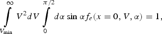
Here the laser is on the left, the target, on the right, and the laser somehow produces a distribution of energetic electrons at the target boundary x = 0 (for instance, the quarter critical surface), which is n e0f e(x = 0,V,α) where α is the polar angle about the x axis and n e0 is the number density at x = 0. We now use the subscript e to distinguish the energetic electron tail from the main distribution function (local and nonlocal parts). Variation is assumed to be only in the x direction. The distribution function is assumed to be azimuthally symmetric, and α ranges from 0 to π/2. We do not consider particles with π/2 < α< π, as these particles, while initially are moving away from the target, do come back due to the electric field. When they return, they may or may not have been energized by the TPD region once more. However the single distribution function f(x = 0,V,α) is assumed to account for this. The distribution is normalized so that
 $$\mathop\int\limits_{V_{\min } }^\infty {V^2 dV} \mathop\int\limits_0^{{\rm\pi} /2} {d{\rm\alpha} \sin}\ {\rm\alpha} f_e \lpar x = 0\comma V\comma {\rm\alpha} \rpar = 1\comma \;$$
where V min is the minimum velocity of an electron considered to be in the energetic tail, n e0 is the number density of these electrons at x = 0, and we have suppressed the dependence on β, the azimuthal angle, because neither f nor the configuration is assumed dependent upon it. This distribution function may be computed, for instance, by the sort of simulation done by Yan et al. (Reference Yan, Ren, Li, Maximov, Mori, Sheng and Tung2012). However, once the electron crosses the x = 0 plane, it is beyond the region of the TPD, and is no longer energized; it only interacts with the dense plasma in front of it.
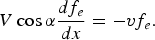
To simplify the calculation, we first neglect the effect of the electric field. Since the energetic electron produced, for instance, by the TPD instability has a velocity very far out on the tail, (i.e., f e(V,α) > f M(V). The kinetic equation is simply
 $$V\cos {\rm\alpha} \displaystyle{{df_e } \over {dx}} = - vf_{e}.$$
Here the particle velocity is simply a parameter; all differentiation is in the spatial domain only. The solution is
 $$\,f_e \lpar x\comma \; V\comma \; {\rm\alpha} \rpar = n_{eo} f_e \lpar x = 0\comma \; V\comma \; {\rm\alpha} \rpar \exp - \mathop\int\limits_0^x {dx^{\prime} \displaystyle{{v\lpar x^{\prime} \comma \; V\rpar } \over {V\cos {\rm\alpha} }}}.$$
The energy flux of the energetic tail as a function of x is then
 $$q_e \mathop\int\limits_{V_{\min } }^\infty {V^2 } dV\mathop\int\limits_0^{{\rm\pi} /2} d {\rm\alpha} \sin {\rm\alpha} \displaystyle{1 \over 2}n_{eo} mV^3 \cos {\rm\alpha} f_e \lpar x\comma \; V\comma \; {\rm\alpha} \rpar .$$
Since energy from the energetic electrons only goes into the thermal electrons, minus the divergence of q e is the heating term in the electron energy equation.
An alternate and perhaps more physically motivated expression for the plasma electron heating would be to substitute ν e for Vcosα and not take the divergence. The obvious sign is taken so that the plasma electrons heat. This choice accounts for the fact that both ν e and V i can contribute to the spatial decay of fe, but only V e gives rise to plasma heating.
It is also useful to point out that even if the plasma has variation in the y and z direction as well, Eq. (4) is basically unchanged except that Vcosαd/dx is replaced with V∂/∂ℓ where ℓ is the unit of length parallel to the velocity chosen, and V is the magnitude of that velocity. One simply performs the integration in as many separated directions as it takes to obtain a sufficiently accurate result (Manheimer et al., Reference Manheimer, Colombant and Schmitt2012).
Let us now consider the effect of the ambipolar electric field. In order to maintain a zero current condition, the plasma sets up an electric field. The fields and the various gradients of both the thermal plasma and energetic component all drive currents. In one dimension, the total current must be zero, and the electric field is chosen to force this zero current condition. The current density of the energetic particles is proportional to n ev, while the energy flux is proportional to n ev 3. Hence, for sufficiently small n e and v e, the energy flux of the energetic electrons in the tail is important while the current is not. This is discussed more fully in the Appendix. To begin with, consider this limit.
We have calculated and used this field in our earlier work on the VDK model. The field to maintain a zero current condition in the local limit (Manheimer et al., Reference Manheimer, Colombant and Goncharov2008) derived nonlocal corrections as well) is given by
 $$\displaystyle{{eE} \over T} \equiv - \displaystyle{e \over T}\displaystyle{{d{\rm\phi} } \over {dx}}=- \displaystyle{1 \over n}\displaystyle{{dn} \over {dx}}+\left[{\displaystyle{3 \over 2} - \displaystyle{{Z_4 } \over {Z_2 }}} \right]\displaystyle{1 \over T}\displaystyle{{dT} \over {dx}}$$
Here T is the electron temperature and Z 4/Z 2 is a Z dependent constant discussed in Manheimer et al. (Reference Goncharov, Sangster, Radha, Betti, Boehly, Collins, Craxton, Delettrez, Epstein, Glebov, Hu, Igumenshchev, Knauer, Loucks, Marozas, Marshall, McCrory, McKenty, Meyerhoffer, Regan, Seka, Skupsky, Smalyuk, Sources, Stoeckl, Shvarts, Frenje, Petrasso, Li, Seguin, Manheimer and Colombant2008), Colombant and Manheimer (Reference Colombant and Manheimer2008; Reference Colombant and Manheimer2009; Reference Colombant and Manheimer2010a; Reference Colombant and Manheimer2010b), and Manheimer et al. (Reference Manheimer, Colombant and Schmitt2012). For our purposes here, we may regard it as being about 3. Clearly, the potential drop across the plasma is on the order of the electron temperature.
Taking account of the electric field, the Vlasov equation for the distribution of the energetic electrons with the Krook collision becomes
 $$V_x \displaystyle{{\partial f_e } \over {\partial x}} + \displaystyle{e \over m}\displaystyle{{d{\rm\phi} } \over {dx}}\displaystyle{{\partial f_e } \over {\partial x}} = - \lpar f_e - f_M \rpar .$$
Now instead of independent variable V x, use
 $$W = \displaystyle{1 \over 2}mV^2 - e{\rm\phi} \lpar x\rpar = \displaystyle{1 \over 2}m\lpar V_x^2 + V_y^2 + V_z^2 \rpar - e{\rm\phi} \lpar x\rpar .$$
Then f e(x,V) becomes f e(x,W). Since the energy of the electrons we are considering is much greater than the electron temperature, that is, much greater than the maximum potential drop across the plasma, we do not have to consider reflection of the particles from the electrostatic potential, and in solving Eq. (9) for V x, we need only concern ourselves with one sign of the square root. The Vlasov equation then becomes
 $$\sqrt {\displaystyle{2 \over m}\lpar W + e{\rm\phi} \rpar } \cos {\rm\alpha} \displaystyle{{\partial f_e } \over {\partial x}} = - vf_e.$$
The collision frequency is now a function of x and the kinetic energy of the particle, E K = (W + eϕ(x)). It is a function of x if W is regarded as the independent variable. The velocity dependent Krook kinetic equation can be integrated as before, and the result for the energy flux of the energetic particles is
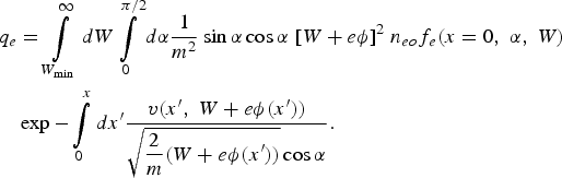 $$\eqalignno{q_e & = \mathop\int\limits_{W_{\min } }^\infty {dW} \mathop\int\limits_0^{{\rm\pi} /2} {d{\rm\alpha} } {{1}\over{m^2}}\sin\alpha\cos\alpha \;[W+e{\rm \phi}]^2 \; n_{eo} f_e \lpar x = 0\comma \; {\rm\alpha} \comma \; W\rpar \cr & \exp - \mathop\int\limits_0^x {dx^{\prime} } \displaystyle{{v\lpar x^{\prime}\comma \; W + e{\rm\phi} \lpar x^{\prime} \rpar \rpar } \over {\sqrt {\displaystyle{2 \over m}\lpar W + e{\rm\phi} \lpar x^{\prime} \rpar \rpar } \cos {\rm\alpha} }}.}$$
However, the correction to the result we have obtained ignoring the electric field is on the order of the temperature divided by the electron energy. Henceforth, we will neglect this correction, although it is certainly possible to include it.
In the Appendix, we consider the case of a denser energetic electron component and show how to calculate the field in this case.
5. SPHERICAL CONFIGURATION
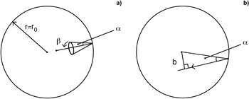
We now consider the TPD position to be at some radius r 0; we are concerned with the propagation of these electrons into the interior of the target. Assume that at r = r 0, the distribution of energetic electrons has the form f e(r = r 0, V, α), where now α is the angle between the velocity of the energetic electron and the radius vector at that particular point on the spherical surface r = r 0, as shown in Figure 1A. The distribution function is assumed independent of the azimuthal angle β. As with the case of the planar target, 0 < α< π/2, those electrons with π/2 < α< π are returned to the target by the electrostatic field, and we assume that f e(r = r 0,V,α) takes this into account. First, we consider the particle kinematics for the spherical configuration, then we consider a calculation of the energy flux of the energetic particles.
(a) A schematic of a distribution of energetic electrons entering the sphere. The distribution function depends on magnitude of velocity V, polar angle α and is independent of azimuthal angle β. (b). The path of the electron entering the circle having impact parameter b.

5.1. Kinematics of Particles for r < r 0 for the Spherical Configuration
Once the electron is inside the TPD surface, r = r 0, it is acted on by a central force, so its angular momentum is conserved. Its impact parameter b is r 0sinα, as in Figure 1B. Since the force is a central force, its entire orbit is in the plane determined by the velocity vector V and the center.
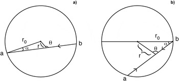
We will first work out the kinetics for the electron orbits in the plane, and then put all the possible planes together so as to get the kinetics in the sphere. Consider the particle as it travels from r 0 to a position r in the circle, where the orbit makes an angle θ with the radius vector, as shown in Figures 2A and 2B, for a particle with small α and for a particle with large α.
(a) Schematic of a particle orbit in the circle for small α, (b). Same schematic but for large α.

Now say the particle distribution function at r = r 0 is n e0f e(V, α) where we will discuss its normalization shortly. Note that in the plane of the orbit, α is a simple polar angle as in two-dimensional polar coordinates. But since there is no β dependence for the spherical case, this means that, f(α) is an even function of α.
Now let us determine the particle distribution function at r and θ and calculate the average particle density and velocity. (We calculate these quantities assuming the particle makes only a single pass through the sphere.) Since the distribution function is constant along a particle orbit, we know that f e(r,V,θ) = f e(r 0,V,α). Note that a particle at r,θ can get there in two separate ways; it can enter the circle from the left, from point a in Figure 2, or from the right, from point b in Figure 2 (for the latter, θ is actually π-θ). However, the velocities are equal and opposite.
To calculate the density, at velocity V, as the particles move into the center of the circle, we want to calculate
 $$\mathop\int \limits_{ - {\rm \pi} }^{\rm\pi} d{\rm\theta} f_e \lpar {\rm\alpha} \rpar = \mathop\int\limits_{ - {\rm\pi} }^{\rm\pi} {d{\rm\theta} f_e } \left( \arcsin \left[{\displaystyle{r \over {r_o }}\sin {\rm\theta} } \right] \right) .$$
where we have used the trigonometric law of sine's to relate α to θ (see Fig. 2).
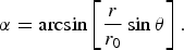 $${\alpha} = \arcsin \left[{\displaystyle{r \over {r_0 }}\sin {\rm\theta} } \right].$$
If f is a smooth function of α, and r is very small, value of the integral is approximately 2πf e(α = 0). Hence, the density increases as the particles approach the center, but it does not diverge, instead it approaches some limiting density, depending on how sharply peaked the angular distribution of α is near α = 0. However, if f(α) is a delta function, δ(α) = δ(rθ/r0), so that all particles point toward the center, then the integral over angle is simple and gives n e(r) = n e(r = 0)r 0/r, as is obviously expected for straight line particle orbits converging to the center of a circle.
However, the odd moments, such as the energy flux being zero, because for every particle at r,θ entering from the left (point a in Fig. 2), there is another particle there with equal and opposite velocity entering from the right (point b in Fig. 2), so the average velocity (and heat flux) is zero.
Now let us consider the spherical situation. For the planar case, we have shown that the orbits lie in a plane due to the fact that the force on the electron is a central force. Hence, every orbit is in some plane, and the spherical case consists of accounting for all of these orbits. We note that every one of these planes passes through the origin. As the particles move along a single plane, their compression as they approach the center is as we have just calculated.
However, particles whose orbits lie on different planes approach each other as they approach the origin. As a function of r, the planes are separated by a distance proportional to r and the angle at which they intersect along their common axis. Hence, as a function of r, there is a spherical compression proportional to 1/r, so for the spherical cases the distribution function is
 $$\displaystyle{{n_{eo} r_o } \over r}f_e \Big( V\comma \; \arcsin \left[{\displaystyle{r \over {r_o }}\sin {\rm\theta} } \right]\Big) .$$
Here θ is the angle between the particle velocity and the radius of the sphere at that point; it is the only angle that enters for the spherically symmetric configuration. This distribution function is normalized so that
 $$\mathop\int\limits_{V_{\min } }^\infty {V^2 dV\mathop\int\limits_0^{\rm\pi} {d{\rm\theta} } } f_e \Big( V\comma \; \arcsin \left[{\displaystyle{r \over {r_o }}\sin {\rm\theta} } \right]\Big) = 1.$$
Hence, for spherical orbits in the central force, there is always a divergence in density proportional to r −1, and it is due to the convergence of the planes containing the orbits as they approach the center. This is an integrable singularity. But again, if all orbits are initially pointed at the center, i.e., f ~ δ(α), the density at the center diverges as r −2 as is of course expected.
5.2. Solution to the VDK Equation in a Sphere
We consider the case where E is neglected. To include this electric field, we can easily extend the calculation from the last section and the in Appendix so as to get an expression for E.
As in the planar case, the solution of the Krook equation is simply the vacuum solution multiplied by an exponential that describes the decay along the orbit (as Eq. (4)). Once again, we will consider particles making a single pass through the sphere expressing the distribution function as a function of α instead of θ; we find that the length of the orbit, starting at r 0 and ending at r is
 $$\ell = r_o \cos {\rm\alpha} \pm \sqrt {r^2 - r_o^2 \sin ^2 {\rm\alpha} }.$$
So that
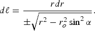 $$d\ell = \displaystyle{{rdr} \over { \pm \sqrt {r^2 - r_o^2 \sin ^2 {\rm\alpha} } }}.$$
Notice that for a given r and α, there are two possible lengths, the longer length, that of the particle entering from point a in, for instance, Figure 2b, and the shorter length, that of the particle entering from point b. The sign of radical in Eq. (17) is chosen so that dℓ is always positive. That is, when the particle just enters, dr is negative, and so the minus sign is chosen in the denominator. However, once the particle passes the radius r = r 0sinα, dr becomes positive, so the plus sign is taken.
The distribution function then becomes the sum of two exponentials, one for the particle taking the long path to reach r, and another for a particle taking the short path. Let us define the quantities
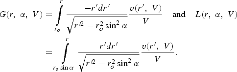 $$\eqalign{G\lpar r\comma \; {\rm\alpha} \comma \; V\rpar & = \mathop\int\limits_{r_o }^r {\displaystyle{{ - r^{\prime} dr^{\prime} } \over {\sqrt {r^{{\prime}2} - r_o^2 \sin ^2 {\rm \alpha} } }}\displaystyle{{v\lpar r^{\prime} \comma \; V\rpar } \over V}} \quad {\rm {and}} \quad L\lpar r\comma \; { \rm\alpha} \comma \; V\rpar \cr & = \mathop\int\limits_{r_o \sin {\rm \alpha} }^r {\displaystyle{{r^{\prime} dr^{\prime} } \over {\sqrt {r^{{\prime}2} - r_o^2 \sin ^2 {\rm \alpha} } }}\displaystyle{{v\lpar r^{\prime} \comma \; V\rpar } \over V}.} }$$
In G, dr is negative, whereas in L it is positive, so each integral is positive.
Then the solution to the Krook equation in spherical geometry is
 $$\eqalign{\,f_e \lpar r\comma \; V\comma \; {\rm \theta} \rpar & = f_e \lpar r = r_o \comma \; V\comma \; {\rm \alpha} \rpar \displaystyle{{r_o } \over r}\lcub \!\exp - \vert G\lpar r\comma \; {\rm \alpha} \comma \; V\rpar \vert \cr &+ \lpar \!\exp - \vert G\lpar r_o \sin {\rm \alpha} \comma \; {\rm\alpha} \comma \; V\rpar \vert \rpar \times \exp - \vert L\lpar r\comma \; {\rm\alpha} \comma \; V\rpar \vert \rcub .}$$
Where necessary, we can relate α to θ by Eq. (13). Note that in the first term, where the particle is moving toward the center, 0 < θ< π/2, whereas for the second term, when it is moving away, π/2 < θ< π. Now let us consider the energy flux inside the sphere, assuming for now that the energetic electrons make only a single pass inside. Note that the G term in Eq. (19) is for particles traveling toward the center, whereas the L term is for particles traveling away from the center. In the absence of dissipation, i.e., ν = 0 the energy flux from these two terms would cancel.
However, in the event of nonzero ν, they no longer cancel. The exponential reduction in the L term above is greater than that of the G term, because the particles have traveled further. Hence, there is a net radial energy flux into the center. It is
 $$q_r = \int \!\!{V^2 dV\mathop\int\limits_0^{2{\rm\pi}} {d{\rm\theta} } \displaystyle{1 \over 2}n_{eo} mV^3 \cos {\rm\theta} f_e \lpar r\comma \; V\comma \; {\rm\theta} \rpar .}$$
By taking the divergence of this energy flux, one can calculate the radial dependence of the heating of the electron plasma by the energetic electrons.
6. ADDITIONAL ASPECTS
We consider two additional aspects for our theory: (1) reenergized particles, and (2) use of the Krook model in conjunction with other models.
6.1. Reenergized Particles
When particles are energized by the TPD instability, some particles move into the core, while others move out into the vacuum. But this latter group of electrons reflects back electrostatically into the plasma, so that the isolated target does not charge up. When they come back, they have the same velocity parallel to the surface, but an equal and opposite velocity perpendicular to the surface. If this were the entire story, treating these electrons would be simple, simply reflect them back into the surface. (In the spherical configuration, the fact that the electrostatic field is a central force gives a very similar result.) The problem is that when they come back, they pass though the TPD region one or more times and may be reenergized. Myatt et al. (Reference Myatt, Zhang, Delettrez, Maximov, Short, Seka, Edgell, Dubois, Russell and Vu2012) pointed this out.
However the simulations of Yan et al. (Reference Yan, Ren, Li, Maximov, Mori, Sheng and Tung2012) would seem to handle this. At the high density boundary, the plasma is in thermal contact with plasma of that density and some particular temperature, 2 keV in their case. At low density the particles are reflected back. Hence, in this simulation of the TPD instability, it ought to reach a steady state as it has a source (the instability) and a sink (the high density plasma that it is in thermal contact with, which removes energized particles). From this steady state (on the picosecond time scale) one could calculate the steady state value of f(V, α) from the simulation, no matter how many times a particle transits the TPD zone. The f(V, α) that we would use on a Krook calculation would be the result of such a simulation.
A more difficult problem of reenergizing electrons, one most likely less amenable to a PIC simulation is with the spherical configuration. Particles that transit the sphere could emerge from the other side and move outward away from the target. They return via the electrostatic field of the target, a field that is both conservative and central, so the particle reenters the target with the same kinetic energy and angular momentum (i.e., impact parameter). If this were the only consideration, one could calculate the additional heating of the particles leaving and reentering by summing up the obvious geometric series.
The problem is that these particles pass through the TPD region at least twice more, so are likely reenergized. Possibly, a simulation like that in Yan et al. (Reference Yan, Ren, Li, Maximov, Mori, Sheng and Tung2012) could model a steady state version of this. To do so it would need to have a source of energetic electrons entering from the high density end, fewer nearly perpendicular to the target (these particles had a longer trip in the sphere), more at grazing angle (these had a shorter orbit in the sphere).
6.2. The Krook Model in Conjunction with Other Models
In the Krook model, the collision frequency is proportional to the ambient density divided by the electron energy to the three halves power. However, there is some uncertainty as to the coefficient. In Manheimer et al. (Reference Manheimer, Colombant and Schmitt2012), we chose the collision frequency in Eq. (2) so that the result matched the more accurate Legendre expansion of the Krook model (i.e., the diffusion model).
Another option is to choose the coefficient of ν, in Eq. (20), so that the Krook result matches, as well as possible, the results of for instance a one million particle Monte Carlo simulation of the type in Yaakobi et al. (Reference Yaakobi, Gotchev, Betti and Stoecki2009). In this way, the Krook expression for energy flux could be used at each fluid time step of the simulation. However, at some small number of times, a Monte Carlo simulation could be performed, and the Krook result could be renormalized so as to match it as well as possible.
7. CONCLUSIONS
The problem of energetic electrons produced via, for instance, the TPD instability has been studied for years in the plasma physics literature. Still there does not seem to be any agreement. For instance, there does not appear to be any agreed upon expression for f e(V, α, r 0) and its dependence on physical parameters (i.e., laser irradiance, bandwidth, etc). Once this is known the next problem is calculating the heating in the target core. Even less is known here; certainly less has been published in the archival literature.
The VDK model that we have developed here is one of several possible approaches. A particular advantage of this model is that it is analytic, fits in well with a fluid simulation, and is economical to use. Consider, for instance, the fact that we may be interested in the heating of a small central region of radius r c ≪ r 0. A Monte Carlo simulation would need very many particles at r 0, just so it could have adequate statistics over a volume (r c/r 0)3 smaller than the spherical volume at which the particles start out. However, this is not a problem for the Krook model where all of this is handled analytically.
It is also worth noting that for use in a fluid simulation, a VDK model, in combination with a Monte Carlo simulation, could be a considerably more powerful tool than either one used alone.
ACKNOWLEDGEMENT
This work was supported by NNSA. The work was done at the Research Support Instruments, Lanham, Maryland, contract number N00173-06-C-2049, in support to the Laser Plasma Branch at Naval Research Laboratory. The author thanks Denis Colombant for a number of very helpful discussions.
APPENDIX: OUTLINE FOR THE VDK CALCULATION OF ELECTRIC FIELD INCLUDING THE EFFECT OF ENERGETIC PARTICLES
Let us consider the thermal and energetic particles only. The electric current of the thermal particles, in the local approximation was calculated in Goncharov et al. (Reference Goncharov, Sangster, Radha, Betti, Boehly, Collins, Craxton, Delettrez, Epstein, Glebov, Hu, Igumenshchev, Knauer, Loucks, Marozas, Marshall, McCrory, McKenty, Meyerhoffer, Regan, Seka, Skupsky, Smalyuk, Sources, Stoeckl, Shvarts, Frenje, Petrasso, Li, Seguin, Manheimer and Colombant2008). There it was shown that
 $$J_{Loc} = - \displaystyle{4 \over {3\sqrt {\rm\pi} }}\left({\displaystyle{{eTn} \over {mv_o }}} \right)\left\{{\left[{\displaystyle{{eE} \over T} + \displaystyle{1 \over n}\displaystyle{{dn} \over {dx}} - \displaystyle{3 \over 2}\displaystyle{1 \over T}\displaystyle{{dT} \over {dx}}} \right]Z_2 + \left[{\displaystyle{1 \over T}\displaystyle{{dT} \over {dx}}} \right]Z_4 } \right\}\comma \;$$
where the notation is as defined in Goncharov et al. (Reference Goncharov, Sangster, Radha, Betti, Boehly, Collins, Craxton, Delettrez, Epstein, Glebov, Hu, Igumenshchev, Knauer, Loucks, Marozas, Marshall, McCrory, McKenty, Meyerhoffer, Regan, Seka, Skupsky, Smalyuk, Sources, Stoeckl, Shvarts, Frenje, Petrasso, Li, Seguin, Manheimer and Colombant2008) except that now ν0 is the average electron collision frequency, which was denoted νe there. As before the Z's are dimensionless numbers calculated by doing various integrals over the Maxwellian distribution function.
The current of the energetic electrons is as calculated in the expression for the energy flux in Eq. (11) except that there is one less energy product and the result is multiplied by –e. Hence, the energetic electron current is
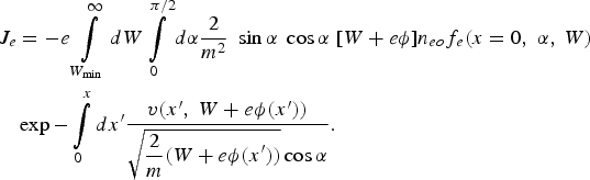 $$\eqalign{J_e & = - e\mathop\int\limits_{W_{\min } }^\infty {dW} \mathop\int\limits_0^{{\rm\pi} /2} {d{\alpha} } \displaystyle{{2 } \over {m^2 }}\;\sin\alpha\;\cos\alpha\;[ W + e{\rm\phi} ] n_{eo} f_e \lpar x = 0\comma \; {\rm\alpha} \comma \; W\rpar \cr & \exp - \mathop\int\limits_0^x {dx^{\prime}} \displaystyle{{v\lpar x^{\prime} \comma \; W + e{\rm\phi} \lpar x^{\prime} \rpar \rpar } \over {\sqrt {\displaystyle{2 \over m}\lpar W + e{\rm\phi} \lpar x^{\prime} \rpar \rpar } \cos {\rm\alpha} }}.}$$
Setting the total current equal to zero, we find a first order differential equation for the electrostatic potential ϕ
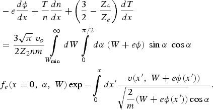 $$\eqalign{&- e\displaystyle{{d{\rm\phi} } \over {dx}}+\displaystyle{T \over n}\displaystyle{{dn} \over {dx}}+\left({\displaystyle{3 \over 2} - \displaystyle{{Z_4 } \over {Z_e }}} \right)\displaystyle{{dT} \over {dx}} \cr & = \displaystyle{{3\sqrt {\rm\pi} \;v_o } \over 2Z_2nm}\mathop\int\limits_{W_{\min } }^\infty {dW} \mathop\int\limits_0^{{\rm\pi} /2} {d{\rm\alpha} } \;\lpar W + e{\rm\phi} \rpar \; \sin\alpha \; \cos\alpha \cr & f_e \lpar x = 0\comma \; {\rm\alpha} \comma \; W\rpar \exp - \mathop\int\limits_0^x {dx^{\prime} } \displaystyle{{v\lpar x^{\prime} \comma \; W + e{\rm\phi} \lpar x^{\prime} \rpar \rpar } \over {\sqrt {\displaystyle{2 \over m}\lpar W + e{\rm\phi} \lpar x^{\prime} \rpar \rpar } \cos {\rm\alpha} }}.}$$
In the body of this paper, we solved this equation by neglecting the right-hand side. If the right-hand side is small, one can use a first order perturbation expansion; that is, use the ϕ(x) obtained by setting the right-hand side equal to zero, insert it into the right-hand side and calculate the perturbation to ϕ. That is, the approach used in Goncharov et al. (Reference Goncharov, Sangster, Radha, Betti, Boehly, Collins, Craxton, Delettrez, Epstein, Glebov, Hu, Igumenshchev, Knauer, Loucks, Marozas, Marshall, McCrory, McKenty, Meyerhoffer, Regan, Seka, Skupsky, Smalyuk, Sources, Stoeckl, Shvarts, Frenje, Petrasso, Li, Seguin, Manheimer and Colombant2008), Colombant and Manheimer (Reference Colombant and Manheimer2008; Reference Colombant and Manheimer2009; Reference Colombant and Manheimer2010a; Reference Colombant and Manheimer2010b), and Manheimer et al. (Reference Manheimer, Colombant and Schmitt2012) where the nonlocal contribution to the electric field, and the energy flux was calculated by a perturbation theory. In this case, one inserts the known function of x, ϕ(x) on the right-hand side of Eq. (A3), perform the x', α, and W integrals to obtain a function of x on the right-hand side. Then integrate Eq. (A3) with this known function on the right.
If perturbation theory is not valid, one can consider the right-hand side to be a function of x and the unknown ϕ. If ϕ is known up to x, we march forward by using that value on the right-hand side, doing the x' integral up to x and the α and W integrals. The right-hand side is then a function of x and ϕ, and one can integrate forward with a simple marching technique.
Let us now perform some order of magnitude estimates. The order of magnitude of the current is
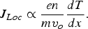 $$J_{Loc} \propto \displaystyle{{en} \over {mv_o }}\displaystyle{{dT} \over {dx}}.$$
And the order of magnitude of the local energy flux is
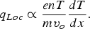 $$q_{Loc} \propto \displaystyle{{enT} \over {mv_o }}\displaystyle{{dT} \over {dx}}.$$
The order of magnitude of the energetic electron current in the Krook approximation is
 $$J_e \propto n_{eo}eV_e\comma \;$$
where V e is a typical magnitude of velocity of an energetic electron. The order of magnitude of the energy flux of energetic electrons is
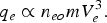 $$q_e \propto n_{eo}mV^3_e.$$
Let us assume that the energy fluxes of the thermal and energetic electrons are roughly equal, so that an important part of the energy is carried by the energetic electrons. If this is so, then the current of the energetic electrons is less than the thermal electron current by about a factor of T/mV e2. Hence, there is a large range of energetic electron energy flux, where this quantity is important or dominant, but where the electric field is determined almost entirely by the thermal electrons.