Epidemiological data are essential to help guide relief and recovery efforts and to protect the health of communities following terrorist attacks and disasters. Both in preparation for and in the aftermath of a terrorist attack or disaster, health care providers, public health planners, and administrators will be called upon to interpret and use such survey and surveillance data.

Although there is an abundance of research that provides reasonable estimates of the likelihood of pathology, both physical and mental, in the general population after mass trauma, Reference Galea, Nandi and Vlahov1–Reference Norris, Friedman and Watson3 there is also an understandable desire on the part of local providers and policy planners for more immediately applicable data, particular to the event, that can be used to guide local response. In many respects, new and customized surveillance or research efforts would be ideal to the taskReference Galea and Norris4 and can probably provide data that most closely reflect the local and specific circumstances of a given mass trauma. However, mounting original data collection efforts after mass trauma events may be challenging. Organizational routines are likely to be disrupted and personnel displaced, and researchers may be unprepared to launch substantial new efforts. In addition, the more pressing needs of those acutely injured may overwhelm interest in developing new projects that assess the health of a population.

Data from existing administrative databases and ongoing surveys or surveillance methods may prove indispensable after mass traumas as a way of providing information that may be useful to emergency planners and practitioners. Existing data collection mechanisms have the advantage of having been established before the mass trauma and of being nested within systems that may, in the best-case scenario, be larger than the disaster's affected area and hence robust to the logistical challenges of the particular local disaster event.

The addition of disaster-specific questions to ongoing surveillance brings its own particular challenges. Standard survey procedures may be unsuited to postdisaster settings. Communications may be disrupted. Displaced populations may put those most acutely affected beyond the reach of telephone or face-to-face interviews. Questions pertinent to a predisaster environment may be less relevant or may be interpreted differently by respondents in postdisaster settings.

In addition to the potential biases introduced by the difficulty of collecting data in postterrorist and disaster environments, analytic methods must address measurement issues such as the lack of uniform definitions among the multiple sources of health information,Reference Noji5 correlation among questions and data sources, and the need to frame questions in appropriate geographic contexts that account for varying levels of exposure. Finally, in the context of complex surveys, weighting and extrapolation of postdisaster data to a target population may become difficult when only a subset of the total survey sample is interviewed about disaster-related outcomes.

The September 11, 2001, terrorist attacks in New York City were in many respects the prototypical large-scale disaster. They were an unanticipated (and unprecedented) event, which shocked the city and the country and which paralyzed normal function in New York City for weeks. Although a number of original research studies were launched in the aftermath of the attacks,Reference Boscarino, Galea and Adams6–Reference Laraque, Boscarino and Battista11 public health authorities quickly recognized that extant surveillance systems may offer unique insights into the health of New Yorkers after these events. To that end, the Centers for Disease Control and Prevention and the New York State Department of Health added questions to address the general population–level behavioral and mental health impacts of the September 11, 2001, terrorist attacks to their ongoing Behavioral Risk Factor Surveillance System (BRFSS)Reference Remington, Smith and Williamson12 telephone survey. Some results from this survey have been reported in aggregate with similar efforts in New Jersey and Connecticut.Reference Melnick, Baker and Adams13

It is the purpose of this article to use this BRFSS effort as a model to introduce and examine some aspects of the challenges involved in analyzing and interpreting existing surveillance data, or new modules appended to existing surveillance efforts, to provide information that is useful in the postdisaster context. We are interested, in particular, in how analytic approach may affect exposure prevalence assessment and measures of association. We compare frequentist survey analytic techniques with Bayesian approaches and examine how such outcomes may affect disaster response and resource allocation and suggest directions for future efforts.

There have been few reports on how best to analyze and interpret such surveys for the purposes of informing postdisaster emergency response efforts. This article should serve as an initial illustration of the implications of different modeling decisions for the purposes of informing future analyses of existing surveillance data in postdisaster contexts, and to highlight the effect analytic approaches may have on the interpretation of such efforts.

Specifically, we compare Bayesian hierarchical modeling methods to standard survey analytic techniques for survey data collected in the aftermath of a terrorist attack. We present results on exposure prevalence and on the outcome of a cross-sectional logistic regression for a possible mental health outcome, and discuss the implications of statistical methodology on efforts to guide disaster relief. We are not aware of published reports to date that have considered a Bayesian approach to postterrorism or disaster survey data.

METHODS

Bayesian Methods

In a Bayesian approach, our 2 main sources of information about parameters of interest (θ) are our prior beliefs or the prior distribution of the parameter (Pr[θ]) and the likelihood of observing the data given the parameter (Pr[y | θ]). Our prior distribution indicates how we believe the parameter would behave if we had no data upon which to base our judgments. The likelihood informs about θ via the data themselves. When we have a lot of data, the likelihood predominates, and our results will essentially be the maximum likelihood estimate. When we have fewer data, the prior distribution has greater influence.Reference Greenland17, Reference Lawson, Browne and Vidal Rodeiro18 The result of combining the prior distribution and the likelihood is called the posterior distribution and follows Bayes theorem:

In a hierarchical (multilevel or mixed) model, we are interested in making inferences on some number of parameters (θ1, …, θk) measured on N units (eg, individuals, subsets, geographic areas, time periods, published studies) that are somehow related or connected by the nature of the problem. We could assume that there is 1 underlying parameter that arises from a single underlying population, in which case the units from which the data arose are uninformative. We could, at the opposite extreme, assume that each unit is a distinct population and should be analyzed separately, leading essentially to a series of descriptive analyses. If, however, we believe that knowing something about some of the units tells us something about the others (eg, data from 9 contiguous geographic areas tell us something about the 10th), then we may assume that the unit data are being drawn from some prior population with unknown parameters much like a random effects model in meta-analysis. At a spatial level, by specifying how the units vary across the population, we can help account for irregular groupings, autocorrelation, and the effects of extreme values in any particular unit.

In our analyses, we specified the subsets or geographic areas that constitute the N units as the New York counties from which samples were drawn. We assumed a normal likelihood for the data in each county x_iz N(θ_z, ςReference Norris, Friedman and Watson2_[e]) i = 1.n_z, z = 1–20 counties, and assumed z distinct but related mean parameters, θz. We took ςReference Norris, Friedman and Watson2_[e] to be unknown and assumed a vague gamma prior for the prevalence estimate and a more informative normal prior for the hierarchical logistic regression model based on maximum likelihood estimation runs of the data.

We used WinBUGS softwareReference Baca Baldomero, Cabanas Arrate, Perez-Rodriguez and Baca-Garcia19 to run 2 parallel Monte Carlo Markov chains with overdispersed initial values for 22,000 iterations. The first 2000 iterations were discarded as a burn-in, and our inferences were based on the final 20,000 iterations. We assessed convergence by examining trace histories for parallel chains, and we used R software20 to conduct the Brooks, Gelman and Rubin, and Geweke convergence diagnostics, as well as the Heidleberger and Welch stationarity test. We present these results at median values for the coefficients with their associated 95% equal-tailed Bayesian credible intervals and their kernel density graphs.

RESULTS

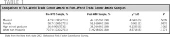
The 1168 (29.96% of total year-long sample) respondents who were asked questions about the World Trade Center in October, November, and December 2001 did not differ in any significant way from the 2731 who were sampled up to the time of the attacks. The 2 groups were similar for county of residence (χ² = 10.5668; df = 21; P = .9567) and age (mean 45.0 pre-WTC, 44.9 post-WTC; t = −0.15; P = .8786).

Table 1 presents additional comparisons. Approximately 48% of respondents were married, 58% were female, 71% were white non-Hispanic, and about one third of the respondents were college graduates.

TABLE 1

Comparison of Pre–World Trade Center Attack to Post–World Trade Center Attack Samples

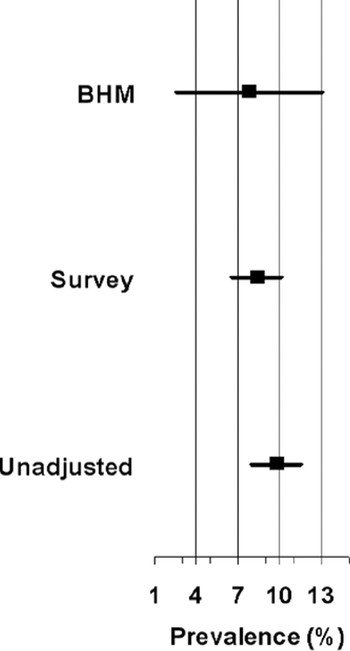
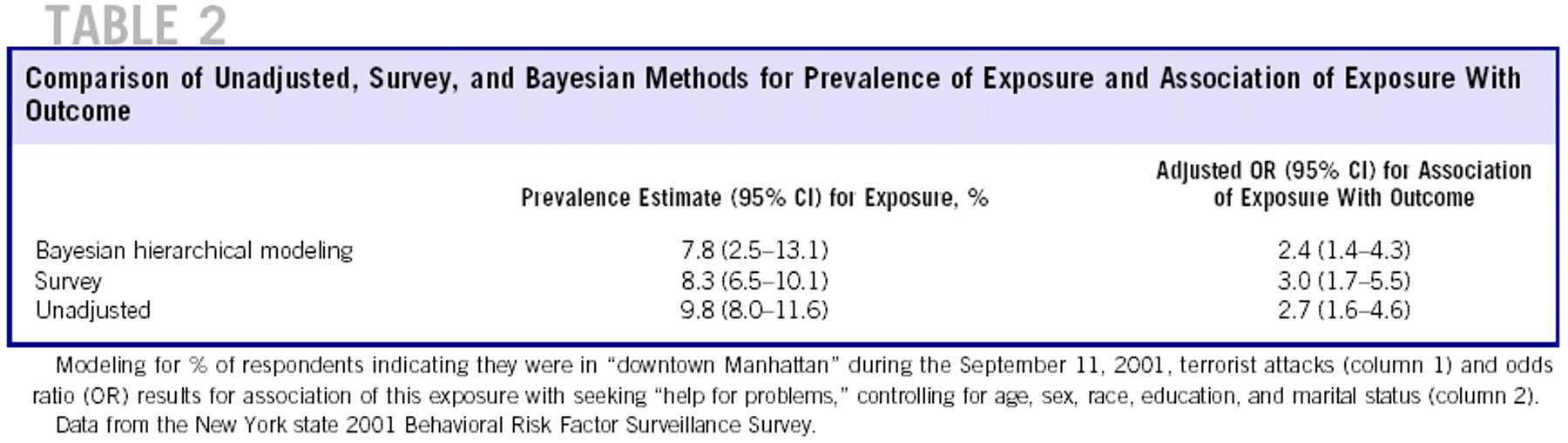
The results for exposure prevalence and the association of exposure with seeking help under each of the 2 approaches are presented in Table 2and Figures 1 and 2. Estimates for the prevalence of exposure to the terrorist attacks of September 11, 2001, varied by the method chosen. Bayesian hierarchical modeling returned the lowest estimate (7.8%), with a credible interval spanning nearly 3 times the range of the CIs associated with both unadjusted and survey procedures. Approximately 15% (0.1502) of the variance in the Bayesian hierarchical modeling approach was related to geographic county (95% credible interval 0.0796–0.236).

FIGURE 1

Forest plot, comparison of direct analysis (Unadjusted), survey procedures using Taylor linearization method (Survey), and Bayesian hierarchical modeling (BHM) for prevalence (percentage and 95% confidence limits) of respondents indicating that they were in “downtown Manhattan” during the September 11, 2001, terrorist attacks (data from the New York state 2001 Behavioral Risk Factor Surveillance Survey)

FIGURE 2

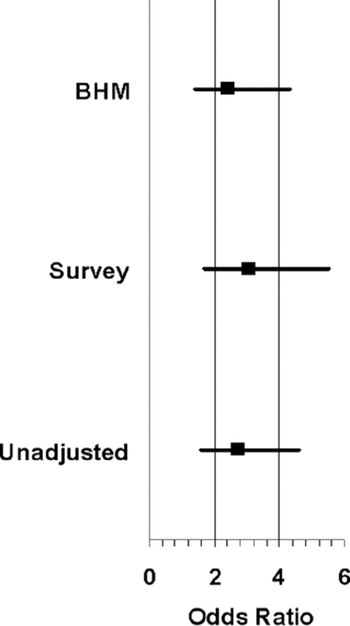
Forest plot comparing direct analysis (Unadjusted), survey procedures using Taylor linearization method (Survey), and Bayesian hierarchical modeling (BHM) for odds ratio results and 95% limits for association of being in “downtown Manhattan” on September 11, 2001, with seeking “help for problems” controlling for age, sex, race, education, and marital status (data from the New York state 2001 Behavioral Risk Factor Surveillance Survey)

TABLE 2

Comparison of Unadjusted, Survey, and Bayesian Methods for Prevalence of Exposure and Association of Exposure With Outcome

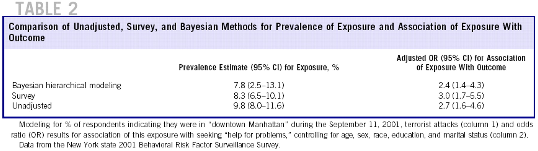
Survey procedures returned a point estimate that was one half of a percentage point higher than the Bayesian estimate with a narrower CI. Unadjusted analyses returned the highest point estimate for prevalence at nearly 10%.

Survey procedures using the reweighted postattack sample returned the highest OR and largest CI for the association of presence in downtown Manhattan on the day of the terrorist attacks with seeking help (Table 1, Fig. 2). Unadjusted analyses returned a smaller point estimate. Bayesian hierarchical modeling returned the smallest point estimate for the OR for association, although in this instance the credible interval was tighter than that associated obtained through using survey procedures.

DISCUSSION

Accurate information in postdisaster settings is essential to guide relief efforts and public health interventions. It has been said that the effort “required to collect the information necessary to provide apt and well-directed aid is more than justified by the improved results.”Reference Noji and Sivertson21 Our results indicate that choice of statistical method may affect the interpretation of such information.

The implications of such differences may be significant. The 6.5% lower bound of the exposure prevalence obtained from a survey analysis approach translates to a minimum of nearly 1 million people in downtown Manhattan on the day of the terrorist attacks. By one estimate, on a typical workday the entire 1.5 million person residential population of Manhattan rises to 2.1 million; the 50,000 employees population of the WTC complex itself was augmented by 100,000 visitors.Reference Bell and Dallas22 Consistent with this estimate, reports put the number of direct victims of this attack at 164,000.Reference Herman, Felton and Susser23 The 2.5% lower bound of the Bayesian credible interval for the prevalence of exposure translates to a minimum of 350,000 people in downtown Manhattan and appears more in line with the likely actual number of individuals exposed.

The wider credible interval from the Bayesian approach may better reflect the uncertainty of the prevalence estimates. By contrast, the tighter credible interval for the OR for association between exposure and seeking help illustrates both an advantage and a difficulty of a Bayesian approach: the choice of a prior distribution. We chose a noninformative (gamma) distribution for the prior in our prevalence calculations to highlight our prior assumption that such an estimate was fraught with uncertainty. For the OR calculation we assumed, based on prior studies of postdisaster pathology, a fairly informative normally distributed prior distribution. Because the posterior distribution in a Bayesian analysis is a weighted average of the likelihood and the prior distribution, placing a restrictive prior distribution on the analysis will necessarily return a tighter credible interval. Sensitivity analyses using less restrictive prior distributions may be helpful in analyzing postterrorism and disaster survey data.

The hierarchical Bayesian approach allowed us to take geography into account and (through the variance partition coefficient) estimate that only about 15% of the probability of exposure was due to geographic residence. This is in line with New York being a commuter city, and could very well be important information in planning and allocating public health resources. We did not calculate a variance partition coefficient for the noncontinuous, non-normal logit-based OR. Approximations existReference Goldstein, Browne and Rasbash24 but are analytically complex to implement and interpret. Sparse cells precluded a hierarchical spatial approach with survey techniques entirely.

Despite these potential advantages, the present study is at best an initial examination of Bayesian approaches to postdisaster population health and these techniques. The reliability and validity of survey methods such as Taylor linearization have been vetted over a long period of time and are widely accepted. As illustrated, Bayesian approaches require choices, particularly about appropriate prior distributions, that may vary from investigator to investigator and that may meaningfully affect the results. An additional example of the use of Bayesian modeling in postdisaster settings may be informative.

In contrast to the evidence on psychopathology, little consensus exists about changes in substance use after mass traumas.Reference Factor, Wu and Monserrate25, Reference Vlahov, Galea and Ahern26 Although some studies have shown an increase in substance use and misuse after mass traumas,Reference Vlahov, Galea and Ahern26, Reference Vlahov, Galea and Resnick27 others have not.Reference Factor, Wu and Monserrate25 One study used Bayesian hierarchical modeling to look at the relation between residential proximity to the terrorist attacks of September 11, 2001, and substance use–related diagnoses in a population of New York City Medicaid enrollees.28

The Bayesian hierarchical analysis drew inferences on the statistical significance of model coefficients for the distance in miles of New York City ZIPcode tabulation areas from the WTC site, controlling for median household income, age, sex, and race. Results indicated that prevalence did indeed vary, but in a predictable fashion, with each 2-mi increment away from the WTC site resulting in 18% more substance abuse diagnoses in the latter part of 2001. This was in contrast to 2000, when each 2-mi increment farther from the WTC resulted in 11% fewer such diagnoses.

CONCLUSIONS

Much remains to be learned about Bayesian approaches to survey data in general29 and postdisaster data in particular. Although it offers potential advantages, the approach has yet to be rigorously tested in the setting of postdisaster population health. A Bayesian approach has been called well suited to the “real-world complexities” of clinical medicine, in which information is scarce, observations are clustered, and results should be intuitive to nonstatisticians.Reference Lewis30 The same may be said for disaster public health.

Disaster care practitioners and planners should be aware that statistical approach may affect point estimates and intervals. Bayesian approaches to survey data may offer potential advantages, particularly in the uncertain environment of postterrorism and disaster settings, but cannot yet be recommended unreservedly. Additional comparative analyses of existing data will help guide our ability to use these techniques for future incidents. The epidemiological information obtained could help improve and inform disaster relief efforts.

Authors' Disclosures The study was supported by Centers for Disease Control and Prevention Health Protection Research Initiative Grant K01 CE000494.

The authors report no conflicts of interest.