1. Introduction
Infant mortality rates today are much lower in industrialized nations than in nations with low rates of industrialization. At the same time, health and mortality worsened during early industrialization in some nations.Footnote 1 A crucial question is whether industrialization in today's poor nations is improving or reducing child health. This question gains urgency when we compare the recent development paths of China – based on highly polluting labor-intensive manufacturing – and India – with more reliance on high-technology employers that provide fewer jobs and fewer negative environmental externalities.
In this study, we examine the relationship between growing manufacturing employment and infant mortality across Indonesian districts from 1985 to 1995, a time of rapid industrialization. An important concern with industrialization as it relates to health, particularly for children, is the pollution generally associated with manufacturing. Thus, in addition to analyzing manufacturing more generally, we also consider whether growth in manufacturing that is concentrated in more polluting industries is particularly harmful to infant health by constructing a harm-weighted index of predicted emissions from manufacturing and estimating its relationship with infant mortality.
Manufacturing growth can have both negative and positive effects on infant health. Factories emit pollutants into the air and water; such emissions are often heavy in poor nations such as Indonesia where pollution regulations are only weakly enforced. Air pollution is a major contributor to the acute respiratory infections that are the most common cause of infant mortality (Romieu et al., Reference Romieu, Samet, Smith and Bruce2002). Also, bringing employees together in factories can increase person-to-person transmission of pathogens. Finally, the urbanization associated with growing industrialization can also negatively impact infant health as person-to-person and water-borne pathogens are more easily transmitted.
Working in the opposite direction, industrialization may bring improvements in housing quality, sanitation, and household pollution, which can improve health outcomes. Similarly, rising incomes can increase access to health care and improve nutrition for mothers and children, in turn lowering death rates (Fogel, Reference Fogel1994). Finally, the urbanization associated with industrialization can also bring children closer to health care than those living in rural areas. In addition, cooking fires – a major source of indoor air pollution that can harm infant health (Smith et al., Reference Smith, Samet, Romieu and Bruce2000) – are less prevalent in urban areas. The net effect of these various positive and negative forces is unclear.
Overall, we find that the relationship between growing manufacturing employment and infant mortality is not significantly different from zero, suggesting that these various forces, to the extent that they exist, balanced each other out for manufacturing generally. However, we find that growth in our measure of harmful emissions from manufacturing is associated with increased infant mortality, suggesting that growth in manufacturing in more polluting sectors is associated with worse health outcomes. The magnitude of the estimated coefficient suggests modest but meaningful reductions in the improvements that were otherwise made in lowering infant mortality during the period. We also find that the harmful emissions appear to disproportionately affect those born to families of less education. Our study follows the same cross-region methodology of historical studies such as that of Rogers et al. (Reference Rogers, Brändström and Edvinsson2004).Footnote 2 A benefit of cross-region studies within a country in comparison to cross-national studies is that we have a larger sample size of regions, more consistent data definitions, and can employ better checks for causality and specification.
Finally, we also explore potential causal channels underlying the observed relationships. We consider a variety of endogenous factors (including housing quality, sanitation, living standards, and access to health care) that may change with industrialization and whose change may help to explain the observed difference in infant mortality. We first analyze whether our industrialization measures predict changes in the potential mediating variables. Then, we add these variables to see if they change the estimated relationship between infant mortality and manufacturing employment and predicted harmful emissions. Although most of these various factors are correlated with infant mortality and manufacturing growth is correlated with changes in several factors, conditioning on these measures does not change our basic results.
2. The setting
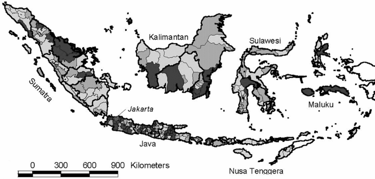
From 1967 to 1997, Indonesia was one of the world's economic success stories, with growth averaging 4.8 per cent per year in real per capita GDP. The population living on one dollar a day dropped from 87.2 million in 1970 to 21.9 million in 1995. Other indicators of development showed progress as well: literacy and immunization rates rose, and infant mortality declined (World Bank, 1999). We study 1985 to 1995, a period of rapid industrialization just preceding the 1997–1998 financial crisis. Figure 1 shows which districts experienced the greatest growth in manufacturing employment. Much of the industrialization was concentrated in West Java near the capital Jakarta. At the same time, there were concentrations of manufacturing growth spread throughout the diverse archipelago.
Industrial development in Indonesia, 1985–1995
Notes: Percentage change in the proportion of manufacturing workers 1985 to 1995 among population aged 18–60 years, district averages, SUPAS. Light gray denotes the bottom third of districts in terms of percentage change in industrialization (that is, essentially none), gray denotes the middle third of districts, and dark gray denotes the top third of districts. The white areas on the map – East Timor and Irian Jaya – are excluded from the analysis.

3. Methods
We compare changes across Indonesian districts from 1985 to 1995 to examine whether infant mortality fell faster or slower in districts with faster growth of manufacturing employment. Our basic methodology is to predict birth-level outcomes using household characteristics, time-varying district characteristics (such as per cent manufacturing), year effects, and district fixed effects. Including district fixed effects in a two-period panel is similar to measuring the effects of changes in the per cent manufacturing, holding constant all fixed factors in the region.
Our first specification assumes that the mortality of infant i in household h in district d at time t depends on average manufacturing employment in the district (%mfgdt), features of the child such as sex and months since birth (Wihdt), features of the household such as its size and demographic composition (Xhdt), features of the district (Zdt), and a random error (εihdt). If we assume the model is linear and the important district characteristics are constant over time, we can eliminate all bias from unobserved district characteristics by adding a vector of district fixed effects (Districtd). For example, if access to a top-quality hospital or the presence of a malarial swamp influences both where factories locate and infant mortality, the stable portion of these regional characteristics will be absorbed by the district fixed effects. Additionally, we include a control for baseline manufacturing employment interacted with it being the later period (manufacturingd85 *year95) to capture if fixed characteristics of the district both led to baseline manufacturing in 1985 and affect the change in infant mortality from then to 1995. Similarly, if fixed characteristics of the district affect both baseline mortality and the growth in manufacturing, we can capture them with a control for baseline infant mortality interacted with it being the later period (mortalityd85 *year95). Thus, we estimate the equation:

In our second specification, we add our harm-weighted index of estimated emissions from manufacturing. The construction of this index is discussed in the next section. By including the index of harmful emissions, we are able to tell if growth in manufacturing employment that is concentrated in more polluting industries is more dangerous for infants.

4. Data and measures
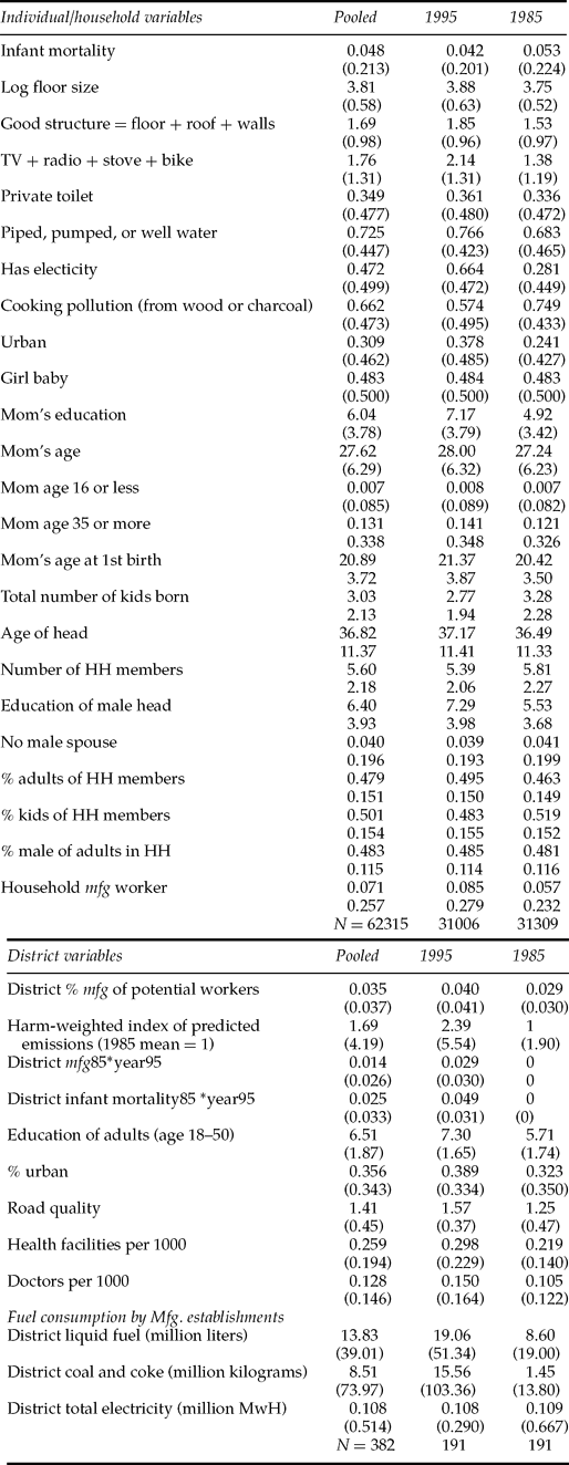
We analyze data from a variety of sources collected by Indonesia's Central Bureau of Statistics. We pool birth, household, and district-level data from the 1985 and 1995 Supas Intercensal Population Survey (Supas) and link these with district-level data from the Susenas National Socio-Economic Survey, the Village Potential Statistics survey, and the Industrial Survey. These datasets are described in the Appendix A1. We combine districts that merged or split between 1985 and 1995 to create a consistent series of districts and drop the (now-former) province of East Timor and the province known during this period as Irian Jaya. Finally, we combine very small, rural districts, merging those districts that are both more than 60 per cent rural and had fewer than 100 births in 1985 within each province. Summary statistics for all variables are presented in table 1.
Summary statistics

4.1 Infant mortality
We analyze infant mortality, measured from the Supas and defined as the death of the child before reaching one year of age. In our data, infant mortality was 53 per thousand births in 1985 and 42 per thousand births in 1995.Footnote 3 This 20 per cent decline in a decade represents rapid improvement (although starting from quite high levels). We include births that took place within the two years preceding each survey.Footnote 4
4.2 District manufacturing employment
Again using the Supas household survey, we count someone as a manufacturing employee if he or she works 20 or more hours a week as an employee or employer in the manufacturing sector. We then calculate total manufacturing employment among those aged 18–60 as a share of total potential employment (# manufacturing workers/total population aged 18–60). To control for possible changes in labor force participation due to industrialization, we focus on the change in manufacturing employment as a share of total adults, which has a smaller level but the same dramatic growth, as manufacturing as a share of workers. From 1985 to 1995, manufacturing as a share of potential employment increased from 3.3 to 5.3 per cent.Footnote 5
Even in large datasets such as the Supas, there is sampling error when examining almost 200 districts. This sampling error is amplified when we measure changes in manufacturing shares. Thus, to address sampling error, particularly in smaller districts, we adjust each district's manufacturing share of potential employment by its ratio of signal to (signal + noise). We can estimate the sampling error (that is, the squared standard error of the district's manufacturing share) because we know the mean and sample size in each district.Footnote 6 This correction is made in the tables presented; results were similar without the correction.
4.3 Harmful emissions from manufacturing
We predict the harm-weighted emissions from manufacturing in each district each year by multiplying the manufacturing employment (Lidt) in each industry (i), district (d), and year (t) times the predicted harm from emissions per employee (Harm/L)i in that industry. The predicted harm per employee in that industry, in turn, is the sum of the predicted pounds of emissions per employee in that industry for each of 322 chemicals ((emissions/L)i, chem) times the estimated toxicity per pound of each chemical (toxicity chem). Formally, we calculate:

For employment by industry, we use employment at the four-digit ISIC level from the Industrial Survey. For pounds of emissions of each chemical per employee in that industry ((emissions/L)i, chem), we use the World Bank's estimates from their Industrial Pollution Projection System (IPPS) (World Bank, 2005). The IPPS estimates are based on reported industrial pollution for several hundred chemicals at each of 200,000 manufacturing firms or factories in the United States in 1987. This data source was chosen based on the quality and quantity of the U.S. data. The IPPS has been used to analyze data in countries as diverse as the Philippines, Mexico, Thailand, Latvia, and India. To measure the toxicity per pound of the predicted emissions (toxicity chem), we use the inverse of 1996 “threshold limit values” (TLVs). TLVs are safe exposure levels as determined by the American Conference of Governmental Industrial Hygienists. Finally, we standardize the index so the average district has a value of 1 in 1985.
The mean across districts of the harm-weighted predicted level of industrial pollution increased 140 per cent (from 1 to 2.4) between 1985 and 1995, largely due to rising manufacturing employment. The mean weighted by the number of births in each district (which better reflects the increase experienced by the average child born) increased by 154 per cent (from 1.3 to 3.3).
A benefit of combining the IPSS estimates of industrial pollution per employee with the TLV estimates of toxicity is that it allows us to weight the predicted pollution by expected harm to health rather than just adding up a physical measure of tons of emissions. A limitation is that we are using a measure of predicted emissions rather than actual. In Appendix A1, we describe our measure in more detail and outline how our estimate of harmful emissions differs from an ideal measure of harm-weighted actual emissions as well as some evidence for its validity. As described further below, we also address measurement error concerns by using actual energy intensity in manufacturing plants in each district to instrument for the harm-weighted predicted emissions index.
4.4 Additional covariates
We include a rich set of household level controls including characteristics of the mother (education, age and its square, as well as dummies for mothers younger than 16 and older than 35, and age at first birth), the child (sex and dummies for months from birth to the survey date), the male head of household (age and its square, education, a dummy if absent), and the household (number of members, age composition, the proportion of adults that are male, and an urban location dummy).Footnote 7 We also include district-level controls for the district's average education of adults (and its square), road quality, and the per cent of the district's population living in an urban area. In the main specification, we treat these as covariates; at the same time, some may be affected by rising manufacturing employment. Thus, in some later analyses, we examine whether they may also be acting as mediating channels; for example, if new factories increase urbanization that, in turn, affects child mortality.
5. Results: industrialization and infant mortality
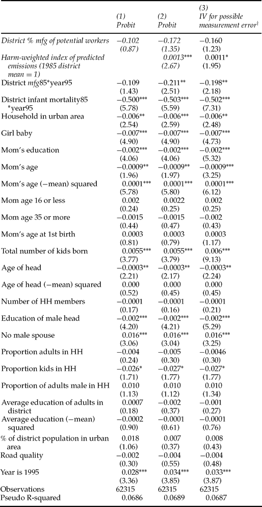
Table 2 presents probit estimates of infant mortality, reported as marginal effects (how the predicted probability of infant mortality changes with a one-unit change of the independent variable). All regressions include district fixed effects and standard errors are adjusted for the clustering of observations at the district level.
Predicting infant mortality

Notes: Probits reported as marginal effects (dp/dx) with district fixed effects and dummies for months elapsed between birth and the survey as described in the text. Z-statistics are robust to clustering at the district level. *significant at 10%; **significant at 5%; ***significant at 1%.
†To address measurement error in the index of predicted emissions as a proxy for actual harmful emissions, we use district-level measures of liquid fuels, coal + coke, and electricity use per district as instruments. First stage results are in table A2.
We find that growth in the share of adults working in manufacturing in a district does not correlate with changes in infant mortality (column 1); it is negative but not significant. The coefficient on manufacturing employment remains insignificant (though less so) when we add the harm-weighted index of predicted emissions (column 2). This coefficient now represents the estimated effect of increasing manufacturing employment, while keeping harmful emissions constant.
The coefficient on harm-weighted predicted emissions index, in contrast, is positive and significant (column 2). That is, those districts whose increased manufacturing employment was concentrated in industries with more predicted harmful emissions per worker experienced a smaller reduction in infant mortality. To interpret the effect size, consider a district that started in 1985 with the mean level of emissions across districts. Growing to the 1995 mean across districts would more than double predicted emissions (from 1 to 2.4).Footnote 8 This increase in emissions predicts 1.8 more deaths per thousand live births – undoing about an sixth of the national average decline in infant mortality achieved that decade. To better reflect the growth in the predicted emissions experienced by the average child born, consider instead the growth in the birth-weighted average of predicted emissions across districts (from 1.3 to 3.3). A district moving from the 1985 to the 1995 birth-weighted average of predicted emissions is estimated to have 2.6 more deaths per thousand (one-quarter of the national average decline in infant mortality).Footnote 9
We also examine whether the impact of increases in predicted harmful emissions varies with characteristics of the household. Jayachandran (Reference Jayachandran2009) finds that the adverse effects of exposure to air pollution on infant and fetal health are greatest in poorer areas. We consider whether there is similar socioeconomic variation in the relationship we find between infant mortality and predicted harmful emissions. While we do not have a direct measure of household income or expenditure, we do have measures of education for the male head of household and the mother which we interact with the index of harmful emissions. The coefficient for the interaction between the education of the male head of household and the harmful emissions index is negative, indicating that the increase in infant mortality associated with rising harmful emissions is lower for those born to families with a more educated male head. The coefficient for the harmful emissions index becomes .0020 (t = 3.78) and the coefficient for the interaction is −.0001 (t = 3.22). This means, for example, that the impact of growth in harmful emissions increases by 80 per cent when moving from a standard deviation above to a standard deviation below the mean for the education of the male head (10.34 to 2.47 years). Interesting, the coefficient of the interaction term is insignificant when the interaction is instead with the mother's education suggesting that the disparity in impact may be working through differences in family income rather than differences in care or information.
Finally, the coefficients on the control variables are generally of the expected sign: infant mortality declines with both mother's and male head's education and children of relatively young or relatively old mothers have higher mortality rates. In addition, infant mortality is higher for those higher in the birth order, and controlling for other factors, girls have lower infant mortality. Before exploring potential causal channels underlying the observed relationships, we first discuss concerns related to causality and to measurement error as well as several specification checks.
5.1 Causality concerns
Statistical problems may arise as endogenous location of people (migration) and endogenous location of factories would imply alternative causality underlying the partial correlations estimated in equations (1) and (2). That is, in Indonesia, as elsewhere, younger and slightly more educated people migrate toward factories. Fortunately, we can deal with the issue of migration because we know both the current district and the district of birth of individuals in our sample. We re-estimated our model-classifying babies by the birth district of the mother. This classification ensures that the results do not depend on non-random mothers moving to be near factory jobs. We also reran analyses dropping all families that have moved and we use industrialization in a mother's birth district as an instrument for the industrialization of the birth district of her baby. The results are robust to these various treatments of migration.
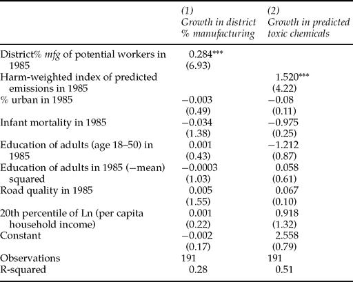
A second concern is that even if the arrival of factories correlates with improved health, the causality could be reversed. For example, Sachs and Malaney (Reference Sachs and Malaney2002) have argued that high mortality and illness due to malaria discourage investment in a region. At the same time, malaria is a major cause of infant mortality. At least during the time period we studied, infant mortality was not a useful predictor of factory location. Appendix table A1 presents district-level regressions that use district characteristics to predict the growth in manufacturing employment and growth in predicted harmful emissions from 1985 to 1995. In both cases, infant mortality in 1985 is not statistically significant and the point estimate is small. These tests, though not conclusive, are suggestive. That is, if factories from 1985 to 1995 did not locate where infant mortality was already low in 1985, then it is less likely that they are locating disproportionately in districts where infant mortality is declining during the 1985–1995 decade. At the same time, regressions such as those in Appendix table A1 are merely suggestive and cannot directly test reverse causality. As noted above, we do capture fixed characteristics of the district that affect both baseline mortality and the growth in manufacturing with the control for baseline infant mortality interacted with it being the later period (mortalityd85 * year95).
5.2 Measurement error
Because our harm-weighted index of predicted emissions is only an estimate of actual emissions, measurement error is a concern. We can address this measurement error if we have another predictor of actual harmful emissions whose own measurement error is uncorrelated with measurement error in how the World Bank IPPS estimates emission of each chemical per worker. Energy intensity in Indonesian manufacturing (specifically, the use of (1) liquid fuels (gasoline, diesel, kerosene, and lubricants), (2) coal and coke, and (3) total electricity) can play such a role. Our measures are actual energy use by manufacturing plants in each district as reported in Indonesia's Industrial Survey.
Formally, we assume that actual harmful emissions in district d at time t (HEdt*) can be proxied with both the IPPS-based index of predicted pollution (Z 1) and by our vector of energy use measures (Z 2):

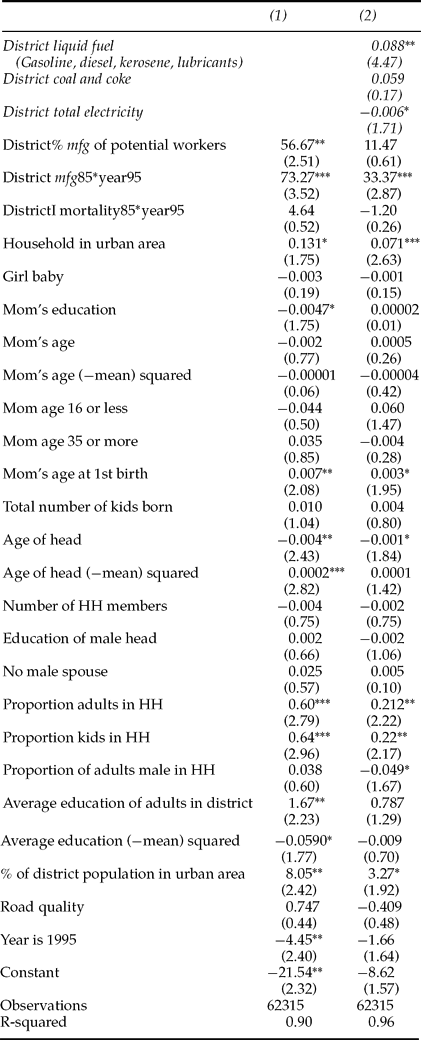
For energy intensity to be an appropriate instrument to correct for measurement error in our harmful emissions measure, it must correlate with predicted harmful emissions. Appendix table A2 presents the first stage of the IV regression. It is clear that districts with energy-intensive industries are also those with high predicted harmful emissions. Our three measures of industrial energy use are jointly highly statistically significant in predicting harmful emissions (with an F-statistic of 24.3).Footnote 10
In column 3 of table 2, we present results where we address potential measurement error by instrumenting for our predicted pollution hazard index with the measures of actual energy use by manufacturing firms in each district. Correcting for measurement error leaves the coefficient on predicted harmful emissions similar (.0011 rather than .0013; the coefficient change is not statistically significant) and it remains statistically significant, now at the 5.2 per cent level.Footnote 11 It should be noted that the actual energy use measure is not harm-weighted, it is simply a summing up of each of three energy types across manufacturing firms in the Indonesian districts. Thus, if anything, we would expect that the estimated coefficient might fall here as we are losing the harm-weighted aspect of our index. As is reported below, the coefficient on harmful emissions is similar though smaller if a predicted measure that is not harm-weighted is used.
5.3 Specification checks
We altered the functional form in several ways to confirm that our results were robust to alternative specifications. We replaced the fixed effects in the probit regressions with the average of district-level variables across 1985 and 1995 (Chamberlain, Reference Chamberlain1980). Separately, we replaced the probit with fixed effects for districts with the conditional logit, where the fixed effects are not estimated, but are implicit. In both cases, results were similar.
We also reran the main regressions dropping all of the potentially endogenous measures of household composition, such as the share of adults, leaving only the predetermined variables of maternal education and the child's age and sex. Results were again robust to these changes with the coefficients for manufacturing employment and predicted harmful emissions nearly identical. Finally, results on the effect of harmful emissions were similar, though a bit weaker if we use simply the sum of tons of pollution instead of our toxicity-weighted measure of harmful emissions. This is to be expected as an index that is weighted by the expected harm associated with the different types of predicted pollution should likely better predict the impact on infant health.
6. Potential causal channels
We consider a variety of endogenous factors that may be affected by district manufacturing growth and may mediate the observed change in infant mortality. We first analyze whether manufacturing growth or changes in predicted emissions predict changes in the potential mediating variables at the household or district level (Appendix tables A3a and A3b, respectively). Then, to test for mediation, we analyze whether including these additional variables changes the estimated relationships (β 1′ and β 2′) between industrialization and infant mortality (table 3). As some of these potentially moderating variables may also have an independent effect on manufacturing employment, the causal interpretations of apparently moderating relations are discussed with care.
Causal channels in predicting infant mortality

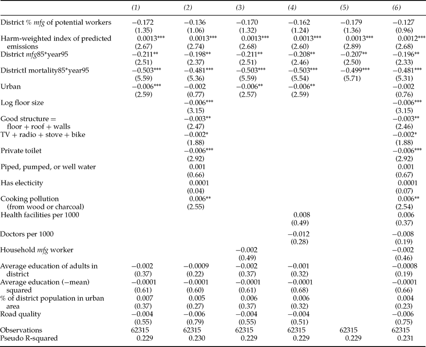
Notes: Probits reported as marginal effects (dp/dx) with district fixed effects, dummies for months elapsed between birth and the survey, and the control variables in table 2. Z-statistics are robust to clustering at the district level. Column (1) replicates results from table 2, column 2. *significant at 10%; **significant at 5%; ***significant at 1%.
6.1 Household level living standards, sanitation, and cooking pollution
One possible benefit of increased industrialization is a higher standard of living. Industrialization both employs people directly and increases employment in related business services and among some suppliers too small to be picked up as manufacturing by our definitions. Higher incomes for these employed people can in turn increase employment for those who provide locally made goods and services. To the extent that migration or capital mobility takes time to equilibrate wages in different regions, industrialization in a local labor market will push up average incomes and living standards. Though we do not have a measure of household incomes, we do have direct measures of various living standards and housing quality.
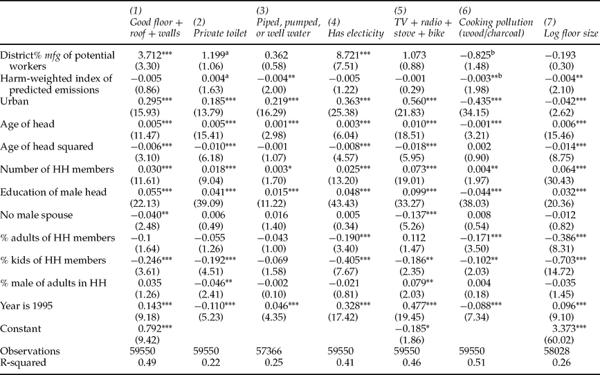
In Appendix table A3a, we show that housing quality (measured as the sum of indicators for a strong floor, walls, and roof), better sanitation (having a private toilet), and electricity grow more rapidly when a district increases its manufacturing employment (columns 1, 2, and 4). Our harm-weighted index of predicted emissions is mixed in terms of predicting better living standards. Growth in manufacturing with higher predicted emissions is associated with declines in the use of wood or charcoal as a cooking fuel (which causes indoor pollution and is associated with increased infant mortality) and with increases in the likelihood of having a private toilet. Yet, it also is associated with decreases in having a high-quality water source (pumped, piped or well water) and decreased housing size.
We add these potential moderating channels into the basic mortality regression in table 3 (the first column replicates table 2, column 2 for comparison). These moderating channels do not change the (insignificant) estimated effects of manufacturing or the higher mortality associated with predicted harmful emissions. At the same time, the results of these additional variables are themselves interesting. As expected, cooking with a polluting heat source predicts higher infant mortality (column 2). The increase is 6 deaths per thousand live births, or almost 15 per cent of the 1995 mean – a large effect. Similarly, high-quality housing structure and a private toilet predict lower mortality (the improvement from having a private toilet is of the same magnitude as the estimated damage from cooking with a polluting heat source).Footnote 12
6.2 Household level manufacturing employment
We also consider manufacturing employment in the household as a causal channel. A household has a manufacturing worker if any adult age 18–60 other than the mother of the focal child works in manufacturing. We exclude mothers because their decision to work in a factory is likely influenced by the presence of a new baby. Because we exclude the mothers, this measure is almost entirely men. A manufacturing worker in the household does not correlate with infant mortality. This is despite the fact that factories employ somewhat advantaged people; in which case, the regressions might overstate the causal effects of household-level manufacturing employment improving living standards or child health.
6.3 Health facilities
There is substantial evidence that high-quality medical care can improve children's outcomes. At the same time, the quality of care in Indonesian health facilities is mixed and it is not clear that expanding low-quality care has much effect on children's outcomes (Barber and Gertler, Reference Barber and Gertler2002). With these cautions in mind, we analyze data on the number of health facilities per thousand residents in the district (a measure that includes integrated and supplemental health centers, maternity houses, and hospitals) and on the number of doctors per thousand residents.
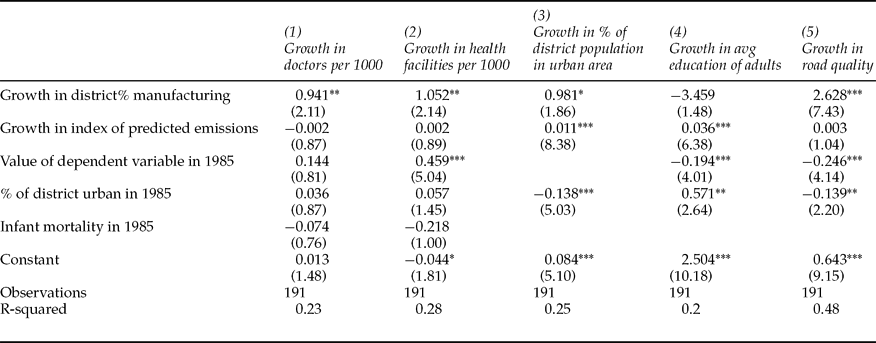
Manufacturing growth is positively correlated with growth in the number of health care facilities and the number of doctors per capita (Appendix table A3b, columns 1 and 2), though growth in manufacturing in more polluting industries does not correlate differentially with these health access measures. Though associated with increased manufacturing in the district, the number of doctors and the number of health facilities per capita does not correlate with infant mortality (table 3, column 4). These results contrast with the more usual result that health facilities are useful (e.g., Frankenberg, Reference Frankenberg1995). Because our measures of health care facilities are not correlated with infant mortality, including them in the regression has no effect on the estimated coefficients on industrialization.
There is also concern about endogenous placement of facilities, where high need may lead to more facilities (Pitt et al., Reference Pitt, Rosenzweig and Gibbons1993; Molyneaux and Gertler, Reference Molyneaux and Gertler2000). When such causality is common, clinic density can often predict worse outcomes due to the decision to place clinics where outcomes are already low. We address this concern partly with our district fixed effects and also by testing for endogenous placement explicitly. We find no evidence that clinics locate in places with high or low infant mortality (Appendix table A3b, columns 1 and 2).Footnote 13
6.4 Industrialization and district characteristics
Industrialization is intertwined with the characteristics of the districts it occurs in. In the previous regressions, we treated urbanization, adult education, and road quality as control variables, which is appropriate if they are determined prior to industrialization. In fact, industrialization can raise incomes, labor demand, and the demand for locally produced goods and services, and all of these changes can increase urbanization, adult education, and road quality. In Appendix table A3b, we document a positive correlation between industrialization and growth in urbanization, adult education, and road quality. If we remove these district-level characteristics from the main regression, though, the main results are nearly identical (table 3, column 5).
6.5 Direct foreign investment
In results not shown, we also explored whether growth in manufacturing associated with DFI (i.e., foreign-owned firms) is differentially associated with infant mortality.Footnote 14 Neither the district share of manufacturing that is foreign-owned nor the share of predicted harmful emissions that is from foreign-owned firms have a statistically significant differential effect on infant mortality. At the same time, it is important to recall that even if foreign-owned manufacturing has no excess effect on infant health relative to other manufacturing, the main effect of manufacturing employment in more polluting industries on infant mortality is negative. Thus, even an estimate of zero on the share that is DFI is still consistent with foreign-owned plants being at least as hazardous as domestically owned plants of similar predicted emissions.
7. Conclusions
While industrialization can bring development and the potential for improvements in living conditions through higher incomes and resources, it also has the potential to have adverse effects on the well-being of youth. As development is a much broader concept than building new factories, the implications of industrialization for living conditions and outcomes, particularly for the young, are important. Because our analysis is across districts (as opposed to cross-national), we are able to compare the experience of babies born during a period of rapid industrialization in Indonesia, who had quite different exposures to the benefits and downsides of being born near factories.
In a companion analysis, we found that increased industrialization in Indonesia from 1985 to 1995 was associated with modestly higher school enrollments and reduced work among young teens (Federman and Levine, Reference Federman and Levine2005). Less optimistically, here we find that although increases in manufacturing employment in general are not associated with changes in infant mortality, manufacturing growth in industries with more harmful emissions is associated with dampening the improvements in infant mortality experienced nationwide during this period. A district moving from the 1985 to the 1995 birth-weighted average of predicted emissions is estimated to have 2.6 more deaths per thousand (equivalent to one-quarter of our measure of the decline in infant mortality). This result suggests that when manufacturing is particularly polluting, the benefits young children receive from improvements in income and living conditions may be outweighed by harm from pollution. Thus, policies to encourage industrial growth should consider pollution levels and cost-effective regulation of industrial pollution. Our results also support policies to encourage safer cooking methods and sanitation.
While a cross-regional study within a single country allows for a larger sample size of regions, more consistent data definitions, and the ability to consider the differential impact of industrialization that is concentrated in more polluting industries, our analysis faces the constraint to generalization of being a case study. Much of our understanding of industrialization's effects on health comes from the vast and detailed historical research on British industrialization. Two centuries later, it is worth examining more recent examples of industrialization to see how children fare. Our analysis though, like its British predecessors, is a case study of just one example of industrialization. It is possible that children in China or Mexico (to take two recent cases) may have had quite different experiences than those in Indonesia, as there are many possible reasons for the effects of industrialization to differ across contexts. Further research comparing the experience of industrialization in Indonesia with industrializations in these countries, for example, should be pursued.
An additional limit to generalization from our findings is that one distinctive feature in Indonesia during this period was its highly centralized tax and expenditures policies. A district that successfully industrialized and, thus, raised more tax revenue did not necessarily have substantially more to spend on health care or clean water. In settings with more decentralized fiscal policies, including Indonesia in recent years, the public health benefits of industrialization that increases local tax revenue are likely to be larger. At the same time, if jurisdictions spend almost all of their potential revenue bidding for manufacturing plants, then total expenditures on health care and clean water can decline nationwide.
Finally, because we lack longitudinal data on households, we cannot examine in detail the effects of manufacturing employment on the children of manufacturing employees. Factory jobs can increase incomes, increase prenatal exposure to chemicals, reduce the length of breastfeeding, and have many other important effects for good and ill. Future research should examine this important question.
Appendix
A1. Data Appendix
Supas: the Intercensal Population Surveys
The primary sources of data are the 1985 and 1995 Intercensal Population Surveys. The Supas 1995 contains data on more than 200,000 households and the Supas 1985 includes 124,000 households. The Supas sample was selected to be representative for each of Indonesia's roughly 300 districts. The survey over-samples smaller districts to increase precision.
Susenas: National Socio-Economic Survey
The National Socio-Economic Survey is an annually repeated cross section and surveyed between 20,000 and 50,000 households per year in the mid-1980s and approximately 200,000 households per year by the mid-1990s. Sampling rules follow those of the Supas. We used the Susenas survey to obtain household consumption data and derive district consumption data for 1995.
PODES: Village Potential Statistics
The Village Potential Statistics survey provides information about the characteristics of villages or urban neighborhood. Roughly 65,000 village heads complete the survey about their villages. Data on health facilities and neighborhood pollution were derived from the 1986 and 1996 Podes surveys. We average the village-level responses to the district level, weighting by population.
SI: the Industrial Survey
The Industrial Survey is an annual census of employers with over 20 employees. Data on factories, employment, and direct foreign investment employment were derived from the 1985 and 1995 Industrial Survey.
A2. Index of harmful emissions
Recall, we calculate:

The pounds of emissions of each chemical per employee in that industry ((emissions/L)i, chem) are the IPPS estimates on reported industrial pollution for 322 chemicals at each of 200,000 manufacturing firms or factories in the United States in 1987. We use IPPS’ lower bound pollution intensities (that assume non-reporting plants had zero emissions), largely due to greater data availability (World Bank, 2005). We combine IPPS estimates of air, land, and water emissions into a single measure.
The toxicity per pound of the predicted emissions (toxicity chem) is the inverse of the American Conference of Governmental Industrial Hygienists consensus estimates of safe occupational exposures (TLV). Specifically, they measure experts’ consensus on the time-weighted average concentrations in air that cannot be exceeded without adverse effects for almost all workers in a normal 40-hour work week. A TLV of one implies a toxicity equivalent to one milligram of sulfuric acid per cubic meter of air. Finally, we standardize the predicted harmful emissions index so the average district has a value of one in 1985 by dividing by the 1985 district mean.
Predicting growth in district manufacturing

Notes: OLS regressions; t-statistics are robust to clustering at the province level. Growth in district characteristics and manufacturing is measured as 1995 value –1985 value. *significant at 10%; **significant at 5%; ***significant at 1%.
Our pollution index has a number of important limitations. It uses average emissions data from American plants in an industry in 1987 (after serious abatement efforts had begun) to predict Indonesian emissions (where regulations are frequently ignored). Furthermore, the measure ignores the differences among Indonesian plants. Emissions figures translate only approximately into human exposure because our index ignores factors such as the distance between a household and the plant, local weather and geographic conditions, the age of the polluting source, and whether the emission is to the air, land, or water. Even when exposure is correct, the medical science translating exposure into biological harm for infants is often uncertain.
In spite of these limitations, the pollution intensities have face validity. For example, the calculated industry-specific indices of pollution risk show that it is more hazardous to be near a chemical or cement plant than an assembly plant. Our index of harmful emissions also has convergent validity, meaning that it correlates with an independent measure of harmful emissions. Specifically, we have data on atmospheric NO2 from the latter period (1995) from the GOME satellite. We linked each district's centroid with the four closest satellite observations. The correlation in the 1995 cross section of districts between our index of harmful emissions and the GOME satellite measure of NO2 was 0.44.
Predicting index of harmful emissions

Notes: OLS Regressions with district fixed effects and dummies for months elapsed between birth and the survey as described in the text. T-statistics robust to clustering at the district level. *significant at 10%; **significant at 5%; ***significant at 1%. F-statistic on the 3 fuel use variables = 24.3.
Does manufacturing predict household characteristics?

Notes: Includes district fixed effects. *significant at 10%; **significant at 5%; ***significant at 1%.
aJointly significant at 5%.
bJointly significant at 1%. t-statistic, z-statistic are robust to clustering at district level.
Does growth in manufacturing employment predict growth in the potential moderators?

Notes: OLS regressions; t-statistics are robust to clustering at the province level. Growth in district characteristics and manufacturing is measured as 1995 value–1985 value. * significant at 10%; ** significant at 5%; *** significant at 1%.