Introduction
Reaction time (RT) refers to the fastest response of a subject to the onset of a stimulus. The RT to a visual stimulus represents the total time taken by a cascade of neural processes to occur beginning with the photoreceptors and finishing with the neural process that triggers the motor response. According to Cao et al. (Reference Cao, Zele and Pokorny2007), the RT has two components, one corresponding to the stimulus-dependent neural response that activates the motor response and the irreducible minimum RT—RT 0—which is mainly determined by the time of the motor response started when the sensory component reaches a response criterion.
RT provides a mean of assessing the effectiveness of the suprathreshold stimulus variables, such as luminance and chromatic contrasts (Plainis & Murray, Reference Plainis and Murray2000; McKeefry et al., Reference McKeefry, Parry and Murray2003), size (Rea & Ouellette, Reference Rea and Ouellette1988; Diaz et al., Reference Diaz, Jimenez del Barco, Jimenez and Hita2001; Parry et al., Reference Parry, Plainis, Murray and McKeefry2004), adaptation luminance (Raab & Fehrer, Reference Raab and Fehrer1962; Rea & Ouellette Reference Rea and Ouellette1988; He et al., Reference He, Rea, Bierman and Bullogh1997), eccentricity (Rains, Reference Rains1963), contrast polarity, and background luminance (Burkhardt et al., Reference Burkhardt, Gottesman and Keenan1987). RT is less sensitive to interindividual variability, and the nonvisual contributions are small in comparison to other measurements, such as simulated realistic tasks (Smith & Rea, Reference Smith and Rea1980) or numerical verification tasks (Boyce & Rea, Reference Boyce and Rea1987; Rea & Ouellette Reference Rea and Ouellette1988).
RT has been investigated since the beginning of 20th century. In a seminal study, Pièron found that, for a given perceptual modality, RT decreases as the stimulus intensity increases, following a power function, which is known as Pièron’s law. RT cannot reach zero because it is limited by a minimum RT or asymptotic level—RT 0 (Medina, Reference Medina2009).
A number of works used RT measurements to study the organization of color processing in the human visual system. Although these investigations have achieved considerable progress in the understanding of visual chromatic processing, sometimes results have been ambiguous and contradictory. Some studies suggest that RT is independent of wavelength (Pollack, Reference Pollack1968; Lit et al., Reference Lit, Young and Schaffer1971; Hita et al., Reference Hita, Gomez, Jimenez del Barco and Romero1986). However, these results were obtained by manipulating the spatial and temporal achromatic transients. Examples of such situations are cases in which these transients were masked by presenting the stimulus in increment mode with no adapting field (Ueno et al., Reference Ueno, Pokorny and Smith1985) or against a dimmer achromatic background (Nissen & Pokorny, Reference Nissen and Pokorny1977). Another example is that used by Ueno et al. (Reference Ueno, Pokorny and Smith1985) who attempted to suppress the achromatic temporal transients by presenting the stimulus against a background flickering with temporal frequencies higher than 15 Hz.
When spatial and temporal luminance transients are removed, for example, by blurring (temporally and spatially) a brief stimulus (McKeefry et al., Reference McKeefry, Parry and Murray2003; Parry et al., Reference Parry, Plainis, Murray and McKeefry2004; O’Donell & Colombo, Reference O’Donell and Colombo2008), RT data strongly depend on wavelength. The results of McKeefry et al. (Reference McKeefry, Parry and Murray2003) and O’Donell and Colombo (Reference O’Donell and Colombo2008) show that RTs are highly sensitive to small deviations from isoluminance. Both studies concluded that the longest RTs correspond to stimuli that isolate the S-cone activity and the fastest responses occurred with L–M-cone–isolating stimuli. In another study, Parry et al. (Reference Parry, Plainis, Murray and McKeefry2004) investigated the effect of the retinal inhomogeneity on chromatic sensitivity and found that the largest difference in RTs between the two chromatic channels occurs in the central foveola due to tritanopia. Consistently, Díaz et al. (Reference Díaz, Jiménez del Barco, Jiménez and Perez-Ocon2001) found that RT, for cone-input variations in either the [S − (L + M)]-cone opponent chromatic channel or the (L–M)-cone opponent chromatic channel, varies in the same way as it does with luminance variations, that is, following Pieron’s law.
Smithson & Mollon (Reference Smithson and Mollon2004) found that when paracentral stimuli are confined to chromatic channels by masking, and presented at equivalent threshold levels, the RT difference between the responses from (L–M) and [S − (L + M)]-cone opponent mechanisms is very small, around 20–30 ms. However, Zele et al. (Reference Zele, Cao and Pokorny2007) suggested that by scaling stimuli through threshold units, RTs from different mechanisms may be confounded due to the fact that the mechanism with poorest sensitivity could be favored.
In another line of investigation, RTs have been used to quantify visual performance as a function of luminance contrast, size, and retinal illuminance (Boyce & Rea, Reference Boyce and Rea1987; Burkhardt et al., Reference Burkhardt, Gottesman and Keenan1987; Rea & Ouellette Reference Rea and Ouellette1988). These authors showed that visual performance improves with increases in target size, luminance contrast, and adaptation luminance. They described a visual performance model as an escarpment and a plateau, which is more pronounced for higher adaptation luminances and larger stimulus sizes. However, the inclusion of color in these models of visual performance has not been considered yet, perhaps because it was thought that the faster responses of the luminance system would mask any effect of stimulus color on subject’s responses. Many psychophysical studies were motivated by the idea that visual perception was impaired at isoluminance, that is, with color information but no luminance information. Nevertheless, after many experiments (for a review see Gegenfurtner, Reference Gegenfurtner2003), it was found evident that the efficiency of visual processing for most tasks is the same for color vision and luminance. In natural scenes, color plays an important role in the speed with which information is processed, for example, a ripe red fruit can be easily detected against green foliage. The way in which luminance contrast and chromaticity are combined to determine RT and the influence of the stimulus parameters is potentially an interesting question.
Our goal was to analyze how the chromaticity and luminance contrast information contained in a stimulus contribute to RTs, considering parameters of the stimulus, such as size and luminance. Thus, we could identify the conditions in which the chromatic information becomes crucial for stimulus detection. Finally, we develop a model that accounts for the effects of color and luminance contrast information on RT, including the balance between chromatic and achromatic contrast. This model is a computational description of the psychophysical mechanisms, with no link to the underlying physiological substrates.
Experiments and data
Stimuli
Stimuli were Gaussian blobs displayed on a Eizo T560i-T monitor at a frame rate of 75 Hz. Patterns were generated using an RGB framestore, which was part of a purpose-built display controller, the Cambridge Research System’s VSG 2:3. The γ values were corrected for each phosphor so as to ensure a linear response between power and luminance. The CIE (Commission Internationale de I’Eclairage) chromaticity coordinates of the red, green, and blue color guns were (0.64, 0.34), (0.30, 0.62), and (0.20, 0.09), respectively.
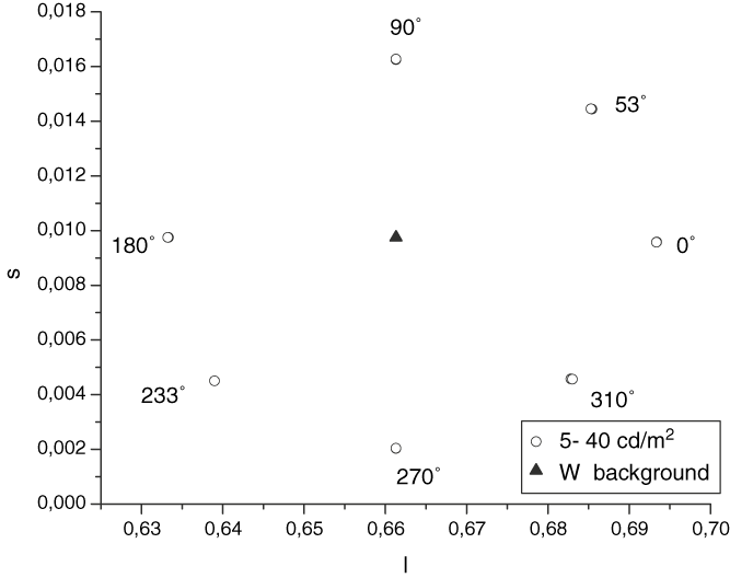
Fig. 1 shows the location of the stimuli on the MacLeod and Boynton (Reference MacLeod and Boynton1979) isoluminant space. The white reference—W—is located at the intersection of the cardinal axes. The chromatic coordinates of the stimulus are found on the line linking the white point—W—with each of the points with (l,s) coordinates. The chromatic stimuli lay on an isoluminant plane that is analogous to the MBDKL color space. In this space: stimuli 0 and 180 deg (the angular azimuth in deg at MBDKL color space: MacLeod & Boynton, Reference MacLeod and Boynton1979; Derrington et al., Reference Derrington, Krauskopf and Lennie1984) are located on the axis that produces only excitation of the L- and M-cones—(L–M)-cone opponent mechanism. The axis corresponding to the [S − (L + M)]-cone opponent mechanism belongs to the conventional tritanopic line. The stimuli called 90 and 270 deg are located on this axis. Theoretically, stimulus modulation along this axis would increase only the quantal catch by the S-cones, leaving the quantal catch by the M- and L-cones unchanged. The remaining stimuli are found in intermediate positions. The stimuli modulated in the cardinal axes appears as reddish, 0 deg, greenish blue, 180 deg, violet, 90 deg, and lime, 270 deg.
The MacLeod–Boynton isoluminant color space showing the location of the seven chromatic axes (Φ = 0, 53, 90, 180, 233, 270, and 310 deg) of the stimuli used in the experiments. The white reference—W—is located at the intersection of the cardinal axes.

The stimulus, which is similar to that used by others (McKeefry et al., Reference McKeefry, Parry and Murray2003; O’Donell & Colombo Reference O’Donell and Colombo2008), consists of a circular patch with a spatial Gaussian profile with the maximum hue modulation at the center. We blurred the stimulus to minimize luminance transients that might occur in the retinal image of the stimulus due to transverse chromatic aberrations (Knoblauch et al., Reference Knoblauch, Arditi and Szlyk1991). The lack of high spatial frequencies in the stimulus precluded chromatic aberration artifacts that can significantly affect these kinds of data.
We tested four different stimulus sizes, which were expressed as the s.d. of the Gaussian blob (0.129, 0.258, 0.522, and 1.045 deg), and 11 Weber luminance contrasts ranging from −40 to 40%, including the isoluminant condition. The experiment was performed with two levels of background luminance, 5 and 40 cd/m2, whose chromaticity coordinates were (x = 0.3449; y = 0.369) and perceived as white by the observers. Note that a background luminance of 5 cd/m2 places the visual system in a range of adaptation where cone–rod interactions may alter the sensitivity and temporal properties of the cone pathway. This was shown by Zele et al. (Reference Zele, Cao and Pokorny2008) using periodic and pulsed stimuli located 7.5 deg away from the center of the visual field. However, we suppose that those interactions will not appear in our experiments because we use stimuli smaller than 1.25 deg presented centrally and thus, stimulating a rod-free area of the fovea (Curcio et al., Reference Curcio, Sloan, Kalina and Hendrickson1991). Our hypothesis is supported by experimental results (Plainis et al., Reference Plainis, Murray and Charman2005) that show a simple monophasic adaptation curve for a foveal stimulus with 1 deg size and 5 cd/m2 adaptation luminance.
For each color direction, we chose one chromaticity (as indicated by the open circles in Fig. 1). For each of these chromaticities, we adjusted luminance, through the range of 11 Weber contrasts from −40 to +40%. We specify the chromatic component of each stimulus according to its projection on the isoluminant plane.
The cone excitation values for the L-, M-, and S-cones were calculated by using the Judd-modified 1931 CIE values in conjunction with the Smith and Pokorny (Reference Smith and Pokorny1972) fundamentals. The square root of the cone contrast—RMSi—was calculated from the equation:

where Δ L/L0, M/M0, and S/S0 are the Weber cone contrasts produced by each isoluminant stimulus on the background (L0, M0, and S0). We characterized the chromatic information with this RMSi value. To characterize the achromatic information, we used the Weber luminance contrast  , where Ls is the luminance of the stimulus and Lb the luminance of the stimulus and the background at isoluminant condition. Likewise, the effects of temporal transients (McKeefry et al., Reference McKeefry, Parry and Murray2003; O’Donell & Colombo, Reference O’Donell and Colombo2008) were minimized by presenting the stimulus with a raised cosinusoidal temporal profile so that hue modulation reached a maximum of 300 ms after stimulus onset. The stimulus remained on for 300 ms and was reduced over the final 300 ms of the presentation using a cosinusoidal temporal profile. The monitor subtended 6.5 deg in width and 9 deg in height when it was placed at a distance of 200 cm from the subject; this distance corresponds to the two smallest stimuli. For the largest stimuli, the monitor was placed at 100 cm, subtending in this case 13 deg in width and 18 deg in height. Head position was maintained by using a chin rest.
The luminance of the stimulus and the background were measured by using a luminance meter Minolta LS 100, and the chromatic coordinates were measured by a color-meter LMT 1200 in the isoluminant condition.
Procedure
Observers were adapted to the display luminance for 5 min before each block of trials. For each observer, the luminance of chromatic stimuli was matched to the background using heterochromatic flicker photometry. The stimulus presented was pulsed on and off at 15 Hz, and the luminance of the stimulus was adjusted until perceptual flicker was minimized. Once the isoluminant condition had been determined, observers were asked to press a button of a response box as soon as they detected the presence of the stimulus. The stimulus presentation was preceded by a random time interval between 1500 and 3500 ms, to prevent the subject from knowing when the stimulus would appear. The time between the presentation of the stimulus and the observer’s response was registered as the RT. The stimulus was turned off by the observer’s response or after 3 s if no response occurred. Once the subject responded, a fixed intertrial interval of 1500 ms was introduced during which the background luminance was presented.
The stimulus parameters (adaptation luminance, color, and size) were chosen randomly from a set of values for each block of 25 trials. Only the luminance contrast sequence was randomized within a block. Each data point was tested 50 times.
Usually, the response–time distribution is similar to a mixture of a Gaussian and an exponential distribution—ex-Gaussian (Luce, Reference Luce1986), and it has been shown that this function fits empirical RT distributions well. To obtain the central tendency of our RT results, we used cutoffs based on the interquartile range (values higher than 75th percentile or lower than 25th percentile of the distribution are discarded). After that, all RT distributions were normal (Kolmogorov–Smirnov one-sample test; STATISTICA) so mean RT was taken as a measure of the central tendency of the distribution. The mean and 95% confidence intervals of RTs were calculated. We used the 95% confidence limits as a measure of RT error bars because it is a robust method of estimating the dispersion.
Observers
Three observers—(BO female, 50 years; MC male, 25 years; and BT male, 25 years)—(one of the authors and two observers naive to the purpose of the experiment) performed the experiments. No comments about the effect of age are available from this study. Subjects were examined for visual defects. Both the Ishihara Color Test and the FM-100 hue test revealed they have normal color vision. Because of her age, we tested the amount of stray light of observer BO by using a straylight meter—Oculus C-Quant (Van Den Berg et al., Reference Van Den Berg, Van Rijn, Michael, Heine, Coeckelbergh, Nischler, Wilhelm, Grabner, Emesz and Barraquer2007). The result of this test shows that this observer presents values within the limits of normality.
The stimuli were viewed binocularly with natural pupils. The protocol of the procedure agrees with the provisions of the Declaration of Helsinki.
Results
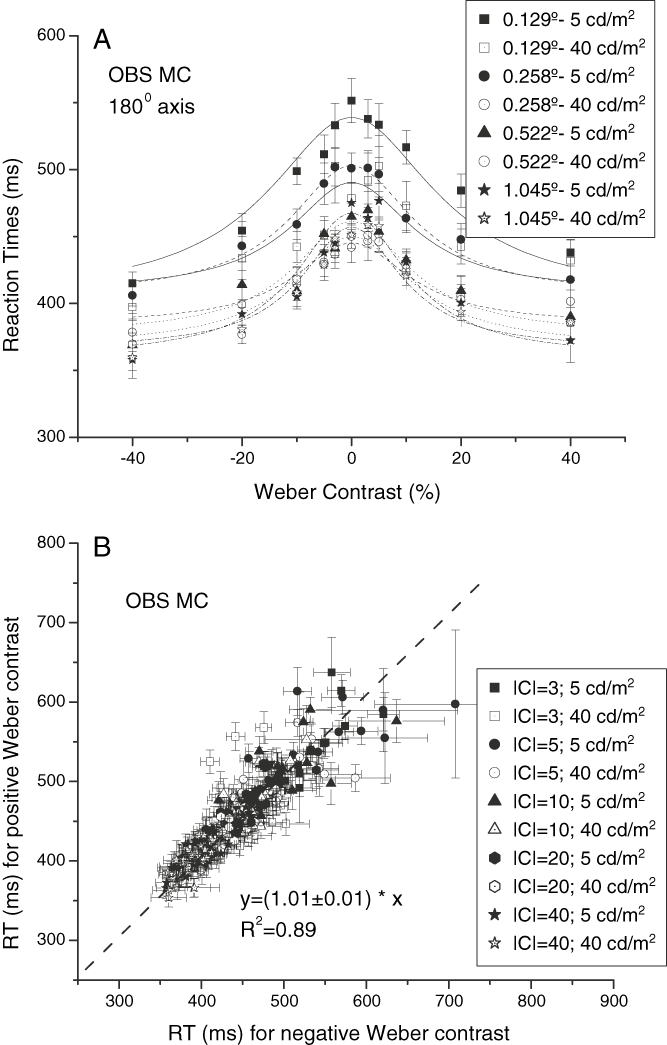
First, we analyzed the hypothesis that Weber luminance contrast polarity has no effect on RT. We quantified the luminance contrast as a % Weber fraction—Weber luminance contrast—in relation to isoluminant condition because it seems to be appropriate for a contrast metric for cone RT (Zele et al., Reference Zele, Cao and Pokorny2007; Vassilev et al., Reference Vassilev, Murzac, Zlatkova and Anderson2009). Fig. 2A (upper panel) shows an example of RT obtained as a function of Weber luminance contrast with both polarities, for observer MC and a 180 deg stimulus (data correspond to all adaptation luminances and sizes). In this plot, the symmetry of the curves of RT versus Weber luminance contrast can be seen. In Fig. 2B (lower panel), we plot RTs obtained with positive luminance contrast as a function of RTs obtained with negative luminance contrast, for the three observers and all stimulus conditions. Data have been fitted by a linear function with a slope close to 1 and 0 intercept (OBS BO: r 2 = 0.96, OBS BT: r 2 = 0.92, and OBS MC: r 2 = 0.89), which would indicate that RT does not depend on luminance contrast polarity, consistently with other findings (Burkhardt et al., Reference Burkhardt, Gottesman and Keenan1987; Rea & Ouellette, Reference Rea and Ouellette1988; Walkey et al., Reference Walkey, Harlow and Barbour2006). However, an analysis of covariance (ANCOVA) would be necessary to study the effects of the stimulus attributes (chromaticity, size, luminance, and absolute luminance contrast) on this correlation. RT data for each observer were subjected to an ANCOVA in a general linear model, with RTs obtained with positive contrast as a dependent variable; RTs obtained with negative luminance contrast as a continuous predictor variable (covariate); and chromatic direction, size, adaptation luminance, and absolute luminance contrast as categorical independent variables (factors). This statistical analysis shows a significant effect of the covariate on the dependent variable, F(1, 11139) = 79970, P < 0.05 for observer BT; F(1, 10143) = 36541, P < 0.05 for observer BO; F(1, 11977) = 1249, P < 0.05 for observer MC, which means that the covariate (RTs obtained with negative contrast) has a linear relation with the dependent variable (RTs obtained with positive contrast). Also, the test of SS whole model as a function of SS residuals presents a value of multiple R 2 equal to 0.96 for observer BT, 0.96 for observer BO, and 0.67 for observer MC. Moreover, RT data for each observer were subjected to a five-way analysis of variance (ANOVA) with chromatic direction, size, adaptation luminance, absolute luminance contrast, and the contrast polarity as main effects (note that we do not include for this analysis the data corresponding to the isoluminant condition). This analysis shows that the sign of luminance contrast is not statistically significant for observers BO: (F(1,21066) = 0.067), BT: (F(1,22785) = 0.055), and MC: (F(1,24133) = 0.097).
(A) RTs as a function of Weber luminance contrast for the chromatic stimuli modulated along the chromatic axis Φ = 180 deg for observer MC, with the size of the stimulus and the adaptation luminance as labeled. (B) RTs for luminance increments above the isoluminant condition as a function of RTs for luminance decrements below the isoluminant condition, for observer MC. The solid line represents a linear fit with a slope equal to 1 (R 2 = 0.89). Other observers show similar behavior. The absolute value of |C| represents both positive and negative contrast values.

According to Burkhardt et al. (Reference Burkhardt, Gottesman and Keenan1987), cone RT is mainly determined by the absolute value of the luminance step independent of the background luminance. In the same way, Cao et al. (Reference Cao, Zele and Pokorny2007) found that the RTs for cone increments or decrements were closely similar, whereas rod RTs were not. Therefore, in the following, we will present the results of RT as a function of the absolute value of Weber luminance contrast—|C|.
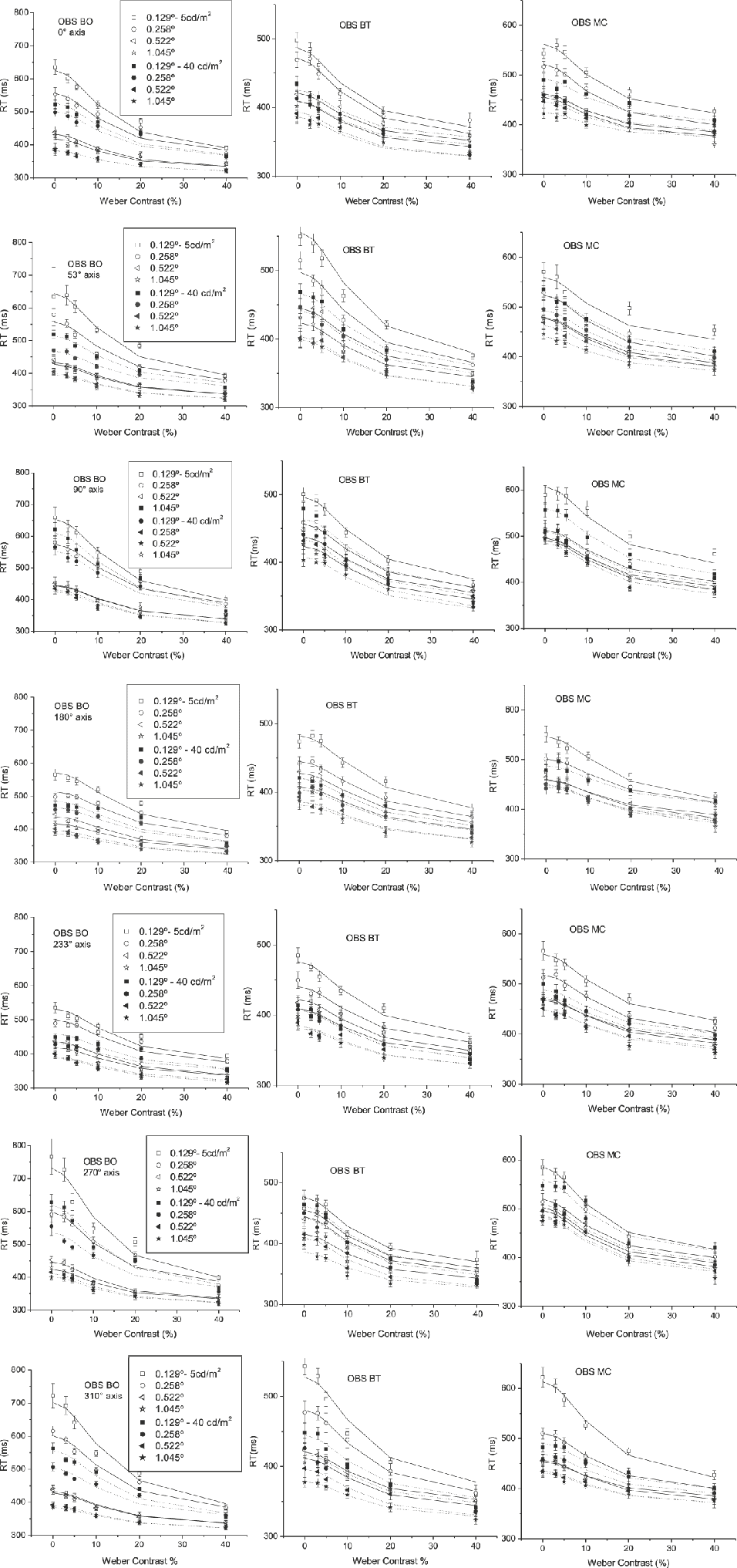
Fig. 3 shows RT as a function of absolute Weber luminance contrast, for the three observers, the two values of adaptation luminance, and the four stimulus sizes. The error bars indicate 95% confidence limits. The solid lines represent the model that will be discussed in section “Model.” The plots show that the longest RTs were obtained at isoluminance for all the stimulus situations, and that they decrease rapidly with increasing luminance contrast, toward an asymptotic value determined by the stimulus configuration. Increasing the adaptation luminance produces a reduction of RT in the same manner for all colors, which is consistent with the hypothesis that color and luminance are processed independently.
Each panel shows the RTs as a function of Weber luminance contrast, using the size of the stimulus and the luminance background as labeled. The data have been fitted using eqn. (3).

Now, we include the values corresponding to the isoluminant condition and performed a new five-way ANOVA with observer, chromatic direction, size, adaptation luminance, and absolute luminance contrast as main effects. This statistical analysis shows a significant effect of the factors observer, F(2, 59771) = 3746, P < 0.05, absolute luminance contrast, F(4, 59771) = 12045, P < 0.05, adaptation luminance, F(1, 59771) = 10315, P < 0.05, size, F(3, 59771) = 10134, P < 0.05, and chromatic direction, F(6, 59771) = 5487, P < 0.05. The differences in RT obtained with sizes of 0.522 and 1.045 deg were not statistically significant. This analysis also shows that the interaction between chromatic direction and luminance contrast is not statistically significant, F(24, 59771) = 0.08, P > 0.05, in agreement with the hypothesis that color and luminance are processed by separate pathways.
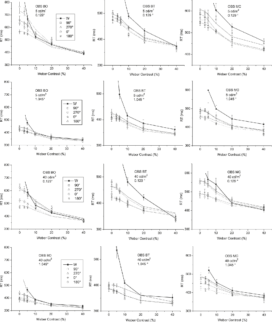
In Fig. 4 we compare the RT values obtained with achromatic and chromatic stimuli. Each column represents one observer and, each row a different experimental situation (0.129 deg and 5 cd/m2; 1.045 deg and 5 cd/m2; 0.129 deg and 40 cd/m2; 1.045 deg and 40 cd/m2, respectively).
RTs as a function of Weber luminance contrast for an achromatic stimulus and chromatic stimuli modulated along four different chromatic axes (Φ = 0, 90, 180, and 270 deg), using different combinations between the size of the stimulus and the luminance adaptation as labeled (0.129 deg, 5 cd/m2; 0.129 deg, 40 cd/m2; 1.045 deg, 5 cd/m2; and 1.045 deg, 40 cd/m2). Data are shown for observers BO, BT, and MC.

An interesting question is how pure chromatic contrast interacts with luminance contrast in the determination of RT. When luminance contrast is zero, RT is purely determined by chromatic information. On the other side of the curve, when luminance contrast is large enough, RT would be exclusively governed by luminance information. However, it is not clear for what range of luminance contrast the transition between these two situations occurs. Results show that for luminance contrasts between 0 and 10 or 20%—depending on the observer— RTs obtained with achromatic stimuli are longer that those obtained with stimuli containing chromatic information. Above this range of luminance contrasts, both curves become indistinguishable. This means that for low values of luminance contrast, chromatic information becomes highly relevant for stimulus detection.
Model
Pieron’s (Reference Pieron and Muller1952) law has been used for many years to describe the variation of RT as a function of size, duration, eccentricity, and luminance and color contrasts. These studies discuss the effects of color and luminance contrast separately. We could not find any study discussing the combined effects of luminance and color contrasts on RT.
The proposed model intends to describe the behavior observed in Fig. 4 by considering the relative effects of luminance and chromatic signals separately. Eqn. (2) shows RT as a function of the reciprocal of luminance contrast (C) using an equation that describes the results of RT for an achromatic stimuli (Plainis & Murray, Reference Plainis and Murray2000).

RT 0 is the asymptotic value of RT, k the steepness of the curve, and n the exponent. According to Plainis and Murray (Reference Plainis and Murray2000), the exponent in eqn. (2) is equal to 1, even though other authors (Mansfield, Reference Mansfield1973) found an exponent of 0.3 for extended sources regardless of the stimulus condition, which is reasonable in the context of a different measure of stimulus strength (Plainis & Murray, Reference Plainis and Murray2000). In eqn. (2), for an isoluminant chromatic stimulus, C is usually expressed by the pooled root mean square representing the cone chromatic contrast-RMSi-(McKeefry et al., Reference McKeefry, Parry and Murray2003; Medina & Diaz, Reference Medina and Diaz2006; O’Donell & Colombo, Reference O’Donell and Colombo2008).
We propose to use a modified formula to fit our results. In this modification, we included a constant—the pure chromatic contrast for the isoluminance condition (RMSi)—added to the absolute Weber luminance contrast (|C|) in the denominator of the second term of the formula. Thus, when C = 0, RT is limited by RMSi. In order to balance the weight of the constant RMSi along the range of Weber luminance contrast, we multiplied |C| by a constant b—free parameter of the model—and RMSi by (1 − b). Therefore, in the new formula, under the hypothesis that the luminance and chromatic channels are independent from one another, we replace Cn of eqn. (2) by  .
Therefore, the formula for the RT model used in Figs. 3 and 4 is:

where g can be understood as a parameter reflecting a shared contrast gain between chromatic and achromatic mechanisms, as we will explain in the next section “Parameter g.”
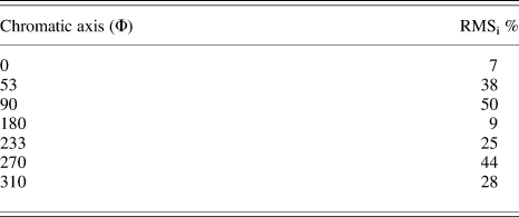
Since RMS cone contrast is dependent on chromatic direction and luminance contrast, we chose the isoluminant RMS cone contrast—RMSi—as a constant term to represent the relative chromatic contrast in each direction. Table 1 shows the chromatic cone contrast values for the selected isoluminant stimuli.
Chromatic cone contrast values—RMSi—for each isoluminant stimulus expressed as a percentage

One complication in the use of the eqn. (3) is the determination of RT 0. As was explained before, RT 0 is the asymptotic value to which RT tends as luminance contrast increases. If we hypothesize that in this situation (large C) the influence of the chromatic component on RT is not significant, then RT 0 can be determined with an achromatic stimulus.
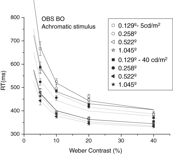
We performed an experiment to determine RT 0 with achromatic stimuli, with chromatic coordinates corresponding to W in Fig. 1. Fig. 5 shows RT as a function of contrast for observer BO. These data were adjusted using eqn. (2), with an exponent n = 1 and the gain k and RT 0 as a free parameters. Table 2 shows the obtained RT 0 by the three observers under all experimental conditions. The differences in RT 0 obtained with sizes of 0.522 and 1.045 deg were not statistically significant.
RTs for achromatic stimuli as a function of Weber luminance contrast. Data for observer BO were adjusted using the equation RT = RT 0 + k/C. Other observers show similar behavior.

RT0 asymptotic values corresponding to an achromatic stimulus for each observer, stimulus size, and adaptation luminance

Analysis of model parameters
In this section, we will explain the procedure we used to obtain the parameters of the model and will discuss their possible meanings in the context of color vision. Because in the present experiment only one chromatic contrast—RMSi—was used for each chromatic direction, any effect introduced by color channels in the model parameters cannot be distinguished from the effect produced by RMSi. To solve this problem, we include for this analysis data from previous experiments, which were performed under identical experimental conditions (O’Donell & Colombo, Reference O’Donell and Colombo2008). These data were obtained for a variety of RMSi, for stimuli modulated along the [S − (L + M)] and (L–M) opponent axes.
Exponent n
Using the present results, we performed two rounds of model fits. In the first round, we fitted eqn. (3) to the RT data with n1, n2, g, and b as free parameters. Results show that the exponents n 1 and n 2 are not statistically different (n 1 = 1.9 ± 0.2 and n 2 = 2.3 ± 0.5). Therefore, we assume that they are equal and used a single n for both |C| and RMSi for the next round of fits. Results indicate that n does not depend on color, size, or adaptation luminance. The only significant effect is given by the observer, F(2,155) = 10.945. However, this effect only explains a small percentage of the variance, and because we hypothesize that n is a constant that represents the sensory modality (in this case the visual mechanisms involved against luminance contrast), we first average n within the different sizes and luminances (1.8 ± 0.2 for subject BO, 2.0 ± 0.1 for BT, and y 2.0 ± 0.2 for MC), and then between subjects, obtaining n = 1.95 ± 0.03. This value of n is consistent with those obtained in a previous work (O’Donell & Colombo, Reference O’Donell and Colombo2008).
Parameter g
As in eqn. (2), the reciprocal of the parameter k is considered as a contrast gain or an index of contrast sensitivity (Plainis & Murray, Reference Plainis and Murray2000). This means the reciprocal of g can be interpreted as a shared contrast gain between chromatic and achromatic information. We ran a new round of fits with n = 1.95 maintaining g and b as free parameters. The ANOVA analysis shows that g depends on chromatic direction, F(6,155) = 56.5, P < 0.05, stimulus size, F(3,155) = 38.7, P < 0.05, and adaptation luminance, F(1,155) = 23.1, P < 0.05. Results show a systematic decrease of g with increasing stimulus size and adaptation luminance. On the other hand, larger values of g are obtained for stimuli modulated on the [S − (L + M)] opponent axis. The post-ANOVA Tukey test shows that the values of g corresponding to the two largest sizes are not significantly different among them. There are statistically significant differences between the values of g obtained with stimuli modulated on (L–M) and [S − (L + M)] opponent axes. Specifically, the stimulus 270 deg presents a smaller g than the 90 deg, while the 53, 233, and 310 deg stimuli present intermediate values but close to that of 90 deg.
The nested design ANOVA in a general linear model analysis for g, done by fitting the model to the RT data of the subsidiary experiment (O’Donell & Colombo, Reference O’Donell and Colombo2008), shows that this parameter presents statistically significant differences only with chromatic direction, F(3,11) = 17.59, P < 0.05, but it does not with RMSi. The values of g are larger for the stimuli modulated on the [S − (L + M)] opponent axis than for stimuli modulated on (L–M) opponent axis, in agreement with the present experiment.
Parameter b
We performed an ANOVA analysis to study the effects of the experimental variables on the parameter b. The analysis indicates that there is a significant effect only for chromatic direction, F(6,155) = 356.43, P < 0.05. We then averaged among size, adaptation luminance, and observers.
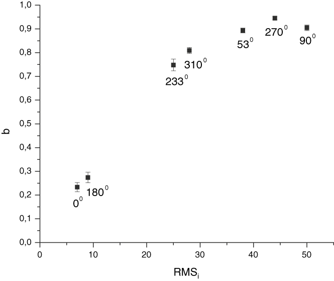
In Fig. 6, we plot b as a function of RMSi. This figure shows that b increases with increasing RMSi. However, one can also observe in the figure that the two smallest values of b correspond to stimuli located on chromatic directions 0 and 180 deg. The values of b obtained for all other directions are much larger than the values for 0 and 180 deg. Interestingly, the variation of b between the second and third data points is much larger than the variation of b along the last five data points. This may suggest that such variation of b would be reflecting a relationship between b and the chromatic channels rather than between b and RMSi. However, because only one chromatic contrast—RMSi—was used for each chromatic direction, we do not know whether the reduced b values for the stimuli modulated on the (L–M)-cone opponent pathway are due to the properties of the (L–M)-cone opponent pathway or simply as a consequence of their low RMSi values. The choice of RMSi values probably exaggerate the differences between mechanisms that have been found in relation to the other variables that were manipulated.
Values of b for each chromatic stimulus obtained using the proposed model given by eqn. (3). Each point represents a mean value over all observers, sizes, and background luminances as a function of isoluminant chromatic contrast—RMSi—Data points were labeled according to their chromatic direction.

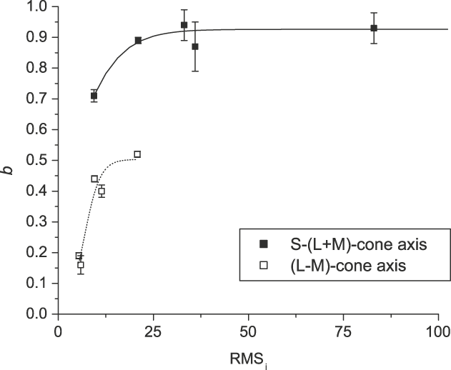
We intend to clarify this ambiguity by including in the analysis a set of data from a previous experiment, which was performed under identical experimental conditions (O’Donell & Colombo, Reference O’Donell and Colombo2008). Now the whole set of data cover a larger range of RMSi such that the values of RMSi for the (L–M) and the [S − (L + M)], cardinal axes overlap one on the other, and thus, we can compare the values of b obtained with stimuli with different chromaticity but similar RMSi values. Fig. 7 shows that b varies in two different ranges depending on the chromatic mechanism. This would strengthen the hypothesis that there are two groups of bs. One group, ranging from 0.7 to 1.0, which correspond to stimuli 90 and 270 deg, and another group ranging from 0.1 to 0.5 corresponding to stimuli 0 and 180 deg. This would mean that the relative weight of luminance contrast in the determination of RT is larger for stimuli modulated along [S − (L + M)] opponent axis than for stimuli modulated along (L–M) opponent axis. Although this model does not have a physiological correlate with any neural substrate, it seems to show that, for equal luminance contrast, stimuli modulated along the (L–M) opponent axis are more salient than those modulated along [S − (L + M)] opponent axis, which would result in shorter RTs (Diaz et al., Reference Diaz, Jimenez del Barco, Jimenez and Hita2001; McKeefry et al., Reference McKeefry, Parry and Murray2003).
Values of b as a function of RMSi for stimuli modulated on each chromatic axis, obtained with the present results and the RT data obtained in a subsidiary experiment (O’Donell & Colombo, Reference O’Donell and Colombo2008).

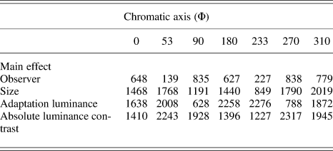
Therefore, we can interpret the data of Fig. 3 as forming groups that are related to the processing channel. For stimuli modulated on the [S − (L + M)] opponent axis, the grouping is mainly governed by size, while the stimuli modulated on the (L–M) opponent axis are mainly grouped by adaptation luminance and size. This last assertion was based on the different values of F shown in Table 3, which contains the results of the four-way ANOVA for each chromatic direction.
Factorial ANOVA outcomes showing the F ratio for the main effects of each chromatic axisFootnote a

a P level < 0.05.
Conclusions
We measured RT to chromatic stimuli for a range of Weber luminance contrasts with different stimulus sizes and adaptation luminances. For all situations, RT decreases with increasing luminance contrast, stimulus size, and adaptation luminance.
We propose a model that considers the contribution of both the chromatic and the achromatic information necessary to trigger the visual response in terms of RT. The model fits the data for all experimental conditions well. Although this model is a computational description of the psychophysical data and does not have a neural correlate, some of its parameters seem to reflect distinct features of the chromatic channels. In particular, the parameter b could be related to the relative contribution of chromatic and achromatic information on RT. As is shown in Fig. 7, the variations of b along the whole range of RMSi occur in two different ranges of values and two well-differentiated groups of b, corresponding to the [S − (L + M)] and (L–M) opponent axes, can be observed. It is known that at the level of the lateral geniculate nucleus, S-cone opponent neurons and (L–M)-cone opponent neurons have separate pathways. While the former would be mediated by the koniocellular layers, the latter would be mediated by the parvocellular pathway. The segregation of these two groups of b could be reflecting these separate pathways, thus supporting the hypothesis that color processing, measured in terms of RT, reflects cone opponent processing (Diaz et al., Reference Diaz, Jimenez del Barco, Jimenez and Hita2001; McKeefry et al., Reference McKeefry, Parry and Murray2003; Parry et al., Reference Parry, Plainis, Murray and McKeefry2004, Reference Parry, Murray and McKeefry2008; O’Donell & Colombo, Reference O’Donell and Colombo2008). When the stimulus is modulated along the [S − (L + M)] opponent axis, more luminance information would be necessary to detect it in relation to the chromatic information, while in the case of stimuli modulated on (L–M) opponent axis, both kinds of information would have similar weights.
Meanwhile, the parameter g depends on adaptation luminance, stimulus size, and chromaticity and does not depend on RMSi. Previous studies (Plainis & Murray, Reference Plainis and Murray2000) have explained the dependence of contrast gain on adaptation luminance; however, the dependence on size and chromaticity deserves consideration in this study. Why would g depend on size and chromaticity? As the stimulus size increases, the number of photoreceptors implicated in the acquisition of information from that stimulus also increases such that if the stimulus is modulated on the [S − (L + M)] opponent axis, the influence of size would be stronger than if it was modulated on the (L–M) opponent axis due to the difference of density or/and the cone distribution on the retina. Mullen & Kingdom (Reference Mullen and Kingdom2002) suggest that the distribution of the (L–M)- and [S − (L + M)]-cone opponency across the visual field are very different. While the (L–M)-cone opponent mechanism can be considered as a foveal specialization, [S − (L + M)]-cone opponency is more uniformly distributed across the visual field and more closely resembles the distribution of the achromatic system. Anatomical studies of the human retina have revealed that L- and M-cones reach their maximum density in the central part of the fovea, whereas S-cones density has a peak around 1 deg of eccentricity and is zero at the tritanopia zone—0.35 deg (Curcio et al., Reference Curcio, Allen, Sloan, Lerea, Hurley, Klock and Millam1990). These inhomogeneities may produce differences between RTs obtained with (L–M)- and [S − (L + M)]-cone opponent RTs, which would be more marked in the central retina. Equating RMSi minimizes but it does not eliminate the faster RTs due to the (L–M)-cone opponent compared to the [S − (L + M)]-cone opponent stimuli according to Parry et al. (Reference Parry, Plainis, Murray and McKeefry2004).
In agreement with Parry et al. (Reference Parry, Plainis, Murray and McKeefry2004), there are differences in gain between (L–M)-cone opponent and [S − (L + M)]-cone opponent mechanisms and, inside this later mechanism, between stimuli at 90 and 270 deg. The rectified model proposed by Sankeralli and Mullen (Reference Sankeralli and Mullen2001) suggests that the processes ON and OFF within the cone opponent neurons of the chromatic pathways are segregated, separating each pole of the cone opponent process. The two opposing submechanisms of the (L–M)-cone opponent mechanism have symmetry between the cones inputs, while the same is not true for the [S − (L + M)]-cone opponent mechanism.
Future work should consider values of g from estimates from physiological studies since the MC, PC, and KC mechanisms have different contrast gains. On the other hand, the use of cone excitation rather than RMSi cone contrast as a metric and the inclusion of opponent and nonopponent components should be considered in future developments of the model.
Finally, we also tested an alternative model in which RMSi was scaled by using multiples of color thresholds (RMSi/RMSit). The results seem to contradict those obtained using RMSi since from this new analysis, it turns out that stimuli lying on the [S − (L + M)]-cone opponent mechanism appear as the most informative (smaller b). It was suggested that when suprathreshold data are expressed in terms of threshold units, the outcomes may appear artificially biased in favor of the mechanism with less sensitivity (Zele et al., Reference Zele, Cao and Pokorny2007). Moreover, this model shows an inconsistent trend of the parameter g, which grows with size. As mentioned by Zele et al. (Reference Zele, Cao and Pokorny2007), the interpretation of RT data may be confounded when expressed in threshold units. Chromatic threshold sensitivity and RT refer to different features of the internal response generated by a visual stimulus.
Acknowledgments
The authors thank Dr. Peter Boyce and Dr. Jose Díaz for advice and discussion of the manuscript, Dra. Viviana Zimmerman for the software, and Elena Bru de Labanda for the statistical support as well as the two unknown referees for their suggestions. This study was supported by a National Agency of Science and Technology (Agencia Nacional de Promoción Científica y Tecnológica—ANPCyT) grant PICT15190 and by a National University of Tucumán (Universidad Nacional de Tucumán—UNT) grant CIUNT E345.